


Calving: A Significant Process
A detailed, semi-quantitative monitoring programme of calving activity was undertaken at Glaciar san Rafael in Chilean Patagonia. This is one of the best field sites for studying short-term calving behaviour because of the great magnitude and frequency of calving. The relationship between regional climate change and the glacier’s historic fluctuations is discussed by Reference Warren,(Warren (1993).
The calving of icebergs from glaciers is a poorly understood process, yet an important one within the global climate system. Current estimates suggest that calving accounts for about 56% of total mass loss from the Greenland ice sheet (Reference Reeh, and Reeh,Reeh, 1994a) and 77% from the Antarctic ice sheet (Reference Jacobs,, Helmer,, Doake,, Jenkins, and Frolich,Jacobs and others, 1992), and it is a significant element in the dynamics and mass balance of many ice Heids worldwide. Interaction between calving topography and proglacial sedimentation can cause non-climatic glacier fluctuations (Reference Mann,Mann, 1986; Reference Alley,Alley, 1991; Reference Powell,, Anderson, and Ashley,Powell, 1991; Reference Trabant,, Krimmel, and Post,Trabant and others, 1991), rendering the resulting glacial geological record of dubious value for palaeoclimate studies (Reference Hillalre-Marcel,, S, and Vincent,Hillaire-Marcel and others, 1981; Reference Meier, and Post,Meier and Post, 1987; Reference Warren,Warren, 1992). Rapid calving in tide water (Reference Hughes,, Ruddiman, and Wright,Hughes, 1987) and fresh water (Reference Andrews,Andrews, 1973; Reference Teller,, Ruddiman, and Wright,Teller, 1987) was crucial to the disintegration of the Pleistocene ice sheets, modulating their response to insolation forcing (Reference Thomas,Thomas, 1977; Reference Mickelson,, Acomb, and Bentley,Mickelson and others, 1981; Reference Pollard,, Berger,, J,, J,, G, and B,Pollard, 1984; Reference Warren, and Hulton,Warren and Hulton, 1990). Calving is also integral to the dynamics of marine ice sheets, such as the West Antarctic ice sheet, which are thought to be unstable (Reference Mercer,Mercer, 1968; Reference MacAyeal,Mac-Ayeal, 1992). Attention has been refocused on large-scale catastrophic calving episodes by the discovery of “"Heinrich events” recorded in the last glacial sediments of the North Atlantic region (Reference Bond,Bond and others, 1992; Reference Andrews,, Erlenkeuser,, Tedcsco,, Aksu, and Jull,Andrews and others, 1994). These indicate that catastrophic calving episodes may occur throughout a glacial period and not simply during its last retreat phase.
Improved understanding of calving dynamics is therefore important for interpretation of the glacial geological record (Reference Powell, and A,Powell and Elverhøi, 1989) and for studies of the interaction between glaciation and climatic change (Reference Hughes,Hughes, 1992; Reference Reeh,Reeh, 1994b). At present, large uncertainties concerning the processes and rates of calving hinder predictions of the likely response of the cryosphere to any future global warming with its implications for sea-level rise (Reference Anderson, and ThomasAnderson and Thomas, 1991; Reference Braithwaite,, Reeh, and Weidick,Braithwaite and others, 1992).
In Patagonia, calving glaciers comprise about half of all outlet glaciers, so high proportions of the total mass loss must be achieved through calving (Reference Warren, and Sugden,Warren and Sugden, 1993). The significance of calving for the dynamics of the Patagonian ice fields was probably much enhanced during glacial periods when there were large proglacial lakes and may have been long, continuous tide-water margins (Reference Hollin,, Schilling,, Denton, and Hughes,Hollin and Schilling, 1981). The regional late-glacial and Holocene chronology of glacier fluctuations developed by Reference Mercer,Mercer (1976, Reference Mercer,1982) rests to a large degree on records from sites at calving glaciers. This questions the validity and use of the chronology for answering questions about the nature of late-glacial climatic change in southernmost South America (Reference Clapperton,Clapperton, 1993; Reference Warren,, Sugden, and Clapperton,Warren and others, in press b).
Glaciar San Rafael
Glaciar San Rafael (46°41′S, 73°50′W) is the lowest-latitude tide-water glacier on Earth. At the end of the 19th century, icebergs from the glacier were regularly towed to Callao, Peru, at 12° S (Reference Weeks, and Campbell,Weeks and Campbell, 1973). The glacier is a western outlet from Hielo Patagònico Norte (northern Patagonia ice field) (Fig. 1), draining about 19% of its total area (Reference Aniya,Aniya, 1988). It flows into Laguna San Rafael in the Parque Nacional San Rafael, terminating at a calving cliff which is 3 km long and 30–70 m high (Fig. 2). Laguna San Rafael is linked to the sea by a narrow channel, the Rio Témpanos, and experiences a tidal range of 1–2 m. Near the terminus, ice velocities during summer 1984 reached 17–22 m d−1 (Reference Kondo, and Yamada,Kondo and Yamada, 1988). Icebergs calve every few minutes (Fig. 3). Icebergs measuring tens and sometimes hundreds of metres in length are common, while exceptional single calving events can involve ice volumes as great as 2 Mm3 (Reference Harrison,Harrison, 1992). After a period of drastic retreat in the 1980s at ≤300 m a−1 (Reference Aniya,Aniya, 1992) the terminus reached a quasi-stable retracted position in the early 1990s. No significant change occurred between the austral summers of 1990/91 and 1992/93 Reference Warren, and Sugden,Warren. 1993).

Fig. 1. Hielo Patagònica Norte (northern Patagonia ice field).
The climate of Chilean Patagonia is similar to that of southeast Alaska but with warmer winters and cooler, windier summers (Reference Mercer,Mercer, 1970). Lying in the “Roaring Forties”, the area is characterized by the frequent passage of rain-bearing storm systems. At sea level at Laguna San Rafael, precipitation exceeds 400mm a−1 (Reference Enomoto,, C, and Nakajima,Enomoto and Nakajima, 1985), while on the accumulation areas of the Patagonian ice fields it may exceed 8000 mm a−1 (Reference Enomoto,, C, and Nakajima,Enomoto and others, 1992). Net accumulation within the San Rafael drainage basin is approximately 3.5 m a−1 and surface ablation rates during the summer are high (Reference Yamada,Yamada, 1987; Reference Kondo, and Yamada,Kondo and Yamada, 1988). producing large volumes of meltwater. Seasonal variations in precipitation and temperature are small, but inter-annual variation is large (Reference Enomoto,, C, and Nakajima,Enomoto and Nakajima. 1985). Consequently, ablation and accumulation seasons vary greatly from year to year and are difficult to define, but the equilibrium-line altitude is about 1200 m (Reference Aniya,Aniya, 1988).
Calving Dynamics: Theoretical Background
The physics of iceberg calving, especially from the submerged part of grounded caking fronts, remains an area of considerable uncertainty (Reference Hughes,Hughes, 1992; Reference Warren,Warren, 1992). Much of our understanding derives from extensive studies of Alaskan calving glaciers, especially Columbia Glacier (Reference Meier,Meier and others, 1980, Reference Meier, and Post,1985; Reference Meier, and Post,Meier and Post, 1987; Reference Krimmel,Krimmel, 1992). These studies have established that, when averaged over long periods (>1 a) there is a between calving speed and width-averaged water depths (Reference Brown,, Meier, and Post,Brown and others, 1982), but that over shorter periods calving correlates more closely with fluctuations in subglacial meltwater discharge (Reference Syvitski, and A,Sikonia and Post, 1980). Data from Columbia Glacier during its current catastrophic retreat at almost 2 km a −1 demonstrate the robustness of the water-depth relation (Reference Meier, and Reeh,Meier, 1994). Calving rates at grounded temperate termini also correlate strongly with ice thickness (Reference Brown,, Meier, and Post,Brawn and others, 1982) and there is some evidence that calving rates from floating termini may also relate to ice thickness (Reference Pelto, and Warren,Pelto and Warren, 1991; Reference Reeh, and Reeh,Reeh, 1994a). Unpublished information from R. LeB. Hooke (1990) has suggested that accumulated longitudinal strain is an important control on calving rates through the promotion of crevassing and stress weakening of the ice, and Reference Powell, and Molnia,Powell (1983) documented calving-speed increases when relict crevasse fields encountered near-terminus extensional fields. Other factors which may exert significant control over calving rates are discussed by Reference Warren,Warren (1992).

Fig. 2. The calving front in February 1992 taken from the observation point on the northern valley side. The photograph was taken shortly before the calving event shown in Figure 3, the location of which is marked.

Fig. 3. A typical subaerial calving event. The location of this event is shown in Figure 2.
Calving produces a bewildering variety of shapes and sizes of icebergs, but there are three main modes of calving, as first discussed by Reference Reid,Reid (1892). The most common is the fracturing of seracs above the waterline which then topple forward or plunge downward. Less frequently, complete sections of the ice front shear off. Submarine blocks also break away and rise to the surface, a process even more poorly understood than subaerial calving. R. LeB, Hooke (personal communication, 1993) suggests a classification of calving events according to the nature of the failure: tensile failure in which a block rotates about an axis near its base or shear failure in which the block slides down with no rotation. He also postulates a third type in which compressive failure or crushing occurs in the base of a block otherwise isolated by crevasses.
In Alaska the submarine parts of calving fronts are typically vertical or overhanging to some degree (Reference Powell,Powell, 1981, Reference Powell,, Milner, and Wood,1988a). However, Reference Hughes,Hughes (1989, Reference Hughes,1992) and Reference Hughes, and Nakagawa,Hughes and Nakagawa (1989) propose that bending shear is the rate-controlling mechanism within calving faces both above and below the waterline, and that, given the different stress regime below the water, there must be a projecting sub-marine ice foot from which calving occurs primarily due to buoyancy forces. This debate goes back to some of the earliest observations of calving glaciers, when Reference Wright,Wright (1892, p. 29) inferred a “projecting foot of ice” and Reference Reid,Reid (1892) and Reference Gilbert,Gilbert (1903) argued the opposite. Reference Reid,Reid (1892) explained observations of bergs rising to the surface at considerable distances from the ice cliff by analogy with a stick thrown obliquely into water which then rises at an angle farther on; he believed that such bergs had travelled underwater before breaking the surface. Apart from its significance for calving processes, this debate is also important in relation to submarine melt rates. The geometry of the submerged part of the ice front affects melt rates through its influence on the interaction of meltwater-discharge plumes with the ice face (Reference Syvitski, and A,Syvitski, 1989).
Methods
This study tests the role of local environmental variables in controlling the magnitude and frequency distributions of calving behaviour. Observational data include calving events, ice velocities in the lower 2 km of the glacier, meteorological data, water depths and proglacial water characteristics.
Calving
During three periods in the austral summers of 1991 and 1992, totalling 32d, standardised observations of all. calving activity between 0800 and 2200h were made from an observation point on the north side of Laguna San Rafael, a position from which about half the front can he seen. A monitoring position on the south side, chosen in order to minimise the potential for duplicate observations, was manned for almost half the time to enable all calving activity to be recorded. Periods 1 and 2 were in 1991 (31 January-13 February and 19–25 February) and period 3 was in 1992 (29 January-8 February).
For each calving event, the time, location and type (subaerial or submarine) were recorded, and a size given based on: (i) the proportion of the ice-cliff height involved, (ii) the size of the resulting iceberg, and (iii) the size and number of waves generated by calving activity. Blocks smaller than about 1m3 were ignored. On the basis of numerous visual estimates, each size category was then assigned a mean volume, enabling semi-quantitative estimates of calving fluxes to be made. The size categories were as follows: small = 25m3, medium = 2500m3, large = 25000m3, extreme = 250000m3. For submarine calving events, the distance between the base of the calving cliff and the emergence position was also recorded. The large composite events proved difficult to classify, involving complex sequences of activity. They typically created such confusion in the immediate proglacial area that distinguishing resurfacing subaerial blocks from submarine calvings was problematic. By contrast, it is possible that some small submarine events went unnoticed because they were inaudible and created minimal disturbance.
An attempt at 24h recording using the sound of calving events yielded spurious results. There were two reasons for this. First, there is no correlation between the audio-volume and ice volume of a calving event. Small events commonly made the loudest noise, akin to rifle fire, while the large submarine calvings were sometimes almost inaudible from the observation point. Secondly, “internal calvings” occur when large seracs fracture and collapse into crevasses close to the front, and these cannot be distinguished from sound alone. For the purposes of this study these internal events were ignored because they did not produce icebergs. The absence of a Right-time record is unfortunate because much activity was heard at night.
Ice velocities
Ice velocities in the glacier’s terminal 2.1km were measured by tracking the movement of prominent seracs positioned around the geometric centre line. The chaotic, intensely crevassed ice surface prohibits a conventional survey. Simultaneous observations were made with a pair of theodolites from survey stations on the north valley-side on a traverse established using electronic distance-measuring equipment. Measurement periods ranged between 1 and 13d from 31 January to 13 February 1991. One or two observations were made each day as weather permitted.
Meteorological data
Precipitation and temperature data were recorded daily by CONAF (national-park) rangers at an abandoned hotel on the north side of Laguna Sati Rafael, about 5 km from the glacier. These observations were later found to be incomplete. Concurrent with the calving monitoring, qualitative observations were made of meteorological conditions, ice conditions on the lagoon, and subglacial discharge as evidenced by upwelling.
Water depths
Water depths in the main body of Laguna San Rafael are known (Reference Nakajima,, J,, Y, and I,Nakajima and others, 1987), but recent rapid retreat has exposed a new channel area. The bathymetry of this area was mapped in February 1992 using an echo sounder. In many places, continuous profiling was impossible due to large quantities of floating ice, so individual soundings were taken.
Proglacial water characteristics
Vertical profiles of temperature, salinity, dissolved oxygen and sediment concentration were measured in Laguna San Rafael during February 1993 using standard oceanographic techniques. Tidal-stage data were provided by a local fisherman.
Data reliability
There are several sources of error in the methods used, chief amongst which are observer error and size-category estimation error. Of the four elements recorded for each calving event (time, location, type and size), the first three have small error but the fourth, based on visual estimates only, has large error margins which cannot be quantified. The semi-quantitative record of daily calving flux provides, at best, order-of-magnitude estimates, it was quantified simply to enable patterns of variability to be analysed. In order to derive estimates of 24h frequencies and fluxes, an assumption had to be made that the nature and speed of calving during the hours of darkness differed insignificantly from those in daylight. This assumption is not testable. However, the amount of audible activity at night, and observations of ice conditions on the lagoon at first light, indicate that calving rates at night are not markedly different from those during daylight hours.
These sources of error were unavoidable. Given the nature of the problem, a semi-quantitative observational approach is the only one that is both feasible and safe. At this field site, the magnitude and variability of activity render the errors in the frequency record insignificant. The much larger errors in the flux estimates are systematic, and therefore the results are internally consistent. The main objective of the calving observations was to analyse the variability of calving behaviour, not to provide an accurate measure of calving flux. Quantitative estimates of the annual calving flux were derived from considerations of mass flux and calving speed.
Table 1. Calving-event frequency and calving flux during the study periods. Calving fluxes were calculated by assigning visually estimated mean values to the observational size categories as detailed in the text.

Results
Calving characteristics
A total of 7279 calving events was recorded during the 32 d. Tables 1, 2 and 3 give the numbers and means of calving events and fluxes, as well as the range of values during each period and from each part of the ice front. Figure 4 shows the fluctuations of subaerial and sub-marine calving activity observed from the observation point on the north side.
Calving from Glaciar San Rafael is continuous, noisy and spectacular. Figures 3 and 5 illustrate two typical calving events, the first a simple “serac fall”, the second a composite event in which subaerial and submarine calvings interacted and triggered further failure. Figure 5 emphasizes the power of the buoyant forces involved. Several of the larger events involved initial upward movement prior to forward and downward collapse, showing that buoyant stress can precipitate failure of coherent sections of the front that span the waterline and reach to the top of the ice cliff. The locations at which fracturing occurred were often clearly related to crevasses immediately behind the calving front. Frequently the release of a large block from the terminal face was followed by the collapse of seracs behind it which had apparently been supported by the frontal block, a sequence of events also described by Reference Harrison,Harrison (1992).
Calving events comprising ice volumes greater than 105m3 were not infrequent. An average of 267 events per day was recorded during daylight hours, yielding a mean daylight calving flux of almost 1.3 Mm3d−1. If calving continues at the same rate at night, then the mean daily event frequency and calving fluxes were 454 d−1 and 2.2Mm3d−1 respecbvely. If it is further assumed that there is little seasonal variation in calving rates, these observations indicate an annual calving flux of 7.92 × 10⁸m3 a−1 or 0.79 km3a−1. Volumetrically, calving activity was focused around the middle of the glacier, and is characterized by large variability from day to day and extreme variability from hour to hour (Figs 4 and 6) in both frequency and magnitude. The number of daylight events ranged between 125 and 545 d−1, while the maximum and minimum recorded daylight fluxes were 1.8 and 0.4 Mm3d−1, respectively.
The largest icebergs were invariably produced by submarine events. This is partly because subaerially calved blocks tend to break up as they enter the water whereas submarine blocks frequently remain intact. Table 4 shows that a disproportionately large share of the total calving flux was produced by submarine calving. Only 7% of the calving events were submarine, but they contributed 27% of the total calving flux. The icebergs produced by such events commonly consisted largely or entirely of bubble-free, dark-blue ice. Many of the submarine icebergs emerged directly in front of the terminal cliff, but some rose to the surface as much as 150m beyond the ice front (Table 5). These emerged vertically and were never observed to have any horizontal momentum. In windless conditions, the emergence of a berg far in front of the cliff typically left the water surface between it and the cliff undisturbed.
Table 2. The number and frequency of calving events during the study periods. “Daylight” = the 14 h d daily observations; daily frequencies were calculated on the assumption that calving continued at the same rate at night

Subaerial and submarine calving were not always associated, but events of one kind often triggered the other. Composite events involving over 1 Mm3 of ice were observed on several occasions in both 1991 and 1992. These sometimes consisted of coherent sections of the calving front from above and below sea level which would typically rotate longitudinally, top or base first, but more rarely would rotate laterally. Such blocks would commonly disintegrate further during the calving event, both before and immediately after entering the water. As a result, large calving events often failed to produce large. Typically, a section of the ice front at which a large event occurred would remain inactive for up to 2 d thereafter.
Table 3. Calving fluxes during the study periods. All flux figures are in m3. “Daylight”= the 14 h of daily observations; daily fluxes were calculated on the assumption that night-time calving continued at the same rate

Meteorological data
Figure 7 shows the meteorological data recorded during the study periods in January and February 1991–92. Temperatures varied little, but precipitation was rather variable.
Ice velocities
Ice velocities increase significantly in the last 1200 m of the glacier where the surface profile is steepest (13°). In this longitudinally convex terminal zone, velocities were 16.8–17.3m d−1 with a mean of 17.0 m d −1. Over two short periods (6h on 31 January 1991 and 19h on 1–2 February 1991), one serac attained velocities of 48.0 m d−1 and 28.0m d−1, respectively. Up-glacier of this section, where the mean surface gradient is 1.5°, surface centre-line velocities were 11.0–12.4 m d−1
Water depths
The bathymetry of the channel area is shown in Figure 8. Water depths average about 200 m in mid-channel, but increase towards the ice front to more than 250 m. The greatest recorded depth is 272 m, at a point near the middle of the ice cliff. In this central section the ice front may he near flotation. The ice front is grounded in deep water along its entire length except at the south end where rocky islets have been exposed by the recent retreat. The southernmost 100 m of the calving cliff stands on bedrock at sea level (Fig. 9). For a further 150m along the cliff, water depths are clearly very shallow, less than 20 m, because the fall of large ice pinnacles is arrested as their base hits the sea floor, while smaller calvings produce sediment-laden plumes of spray Large icebergs calved in this section cannot float away but remain grounded at the ice front until melting reduces their draught.

Fig. 4. Calving activity observed from the northern observation point during the study periods, showing the proportions of total daylight fluxes. contributed by different size categories due to (a) subaerial calving and (6) submarine calving. The location of the observation points on the north and south valley sides is shown in Figure 8.
Table 4. The percentages of frequency and flux contributed by submarine calving

Proglacial water body
The oceanographic results will be fully reported elsewhere (paper in preparation by R. D. Powell and others). Salinity is uniformly low, between 14 and 16 ppt throughout Laguna San Rafael, and concentrations of suspended sediment are remarkably low for a cool-temperate proglacial situation, a mere 13 mg l−1 (cf. Powell, 1991). Spatially, water temperatures vary little in the lagoon. Vertical profiles 200 m from the ice front in a water depth of 175m show temperatures consistently between 5.5° and 6.5°C. There is no evidence of stratification in any of the profiles; the water column is entirely mixed.
The dominant outlet for subglacial meltwater lies approximately one-third of the way along the ice front from the north margin and produces a roughly circular zone of surface turbulence about 300m in diameter. There is also a strong outflow adjacent to the north bank. The location of the main upwelling, centred about 200m in front of the ice cliff, was stable during the summers of 1991–93. It was noted by Reference Ohata,, H,, H, and Nakajima,Ohata and others (1985). and so has probably persisted in the same position relative to the ice front throughout the last 10a of rapid retreat. Continuous, powerful upwelling of the meltwater jet frequently produces superelevation or boiling (cf. Reference Syvitski, and A,Syvitski, 1989) thai operates in pulses as distinct plumes rise in slightly different locations within turbulent zone.

Fig. 5. A combined subaerial submarine calving event. The sequence of events shown took about 90 s. Note the large submarine blocks rising 20–30 m out of the water between a and b and between d and c.
Table 5. The distance in front of the calving cliff of submarine events

The current in the central outlet area keeps it free of brash ice and icebergs by carrying them out into the lagoon. Evacuation speeds are typically about 1–1.5 m s−1, though sometimes greater than 4 m s −1 (Reference Harrison,Harrison, 1992). By contrast, icebergs calved from the southern half of the ice front often have a residence time near the ice front of several hours. Exceptions to this occur after periods of heavy precipitation, when temporary meltwater outlets operate in many locations along the ice cliff, and when a strong katabatic wind is blowing. The existence of numerous additional low-volume meltwater outlets is suggested by the meltwater runnels commonly observed on icebergs, thought to be formed by vertical flow up the submerged part of the front (Reference Powell,, Dowdeswell, and Scourse,Powell, 1990).

Fig. 6. Two sample daily records of calving activity along the whole ice front illustrating the hour-to-hour variability, a. 1 February 1992. b. 8 February 1991. Note that scales for a and b are different.
Periodic catastrophic drainage of marginal lakes also contributes to the glacier’s hydrological regime. Exceptional outflow at the terminus caused by marginal lake drainage was noted by Reference Ohata,, H,, H, and Nakajima,Ohata and others (1985). During the course of this research several marginal lakes, one with an estimated volume of at least 105 m3, were observed to drain in the space of a few hours.

Fig. 7. Daily precipitation and minimum daily temperature recorded at the abandoned hotel by CONAF during the study periods.

Fig. 8. Preliminary bathymetry of the recently deglaciated channel area of Laguna San Rafael(ND = no data), and the locations of the two observation points on the north and south sides.

Fig. 9. The southern half of the calving front in February 1992.
Analysis
Calving-speed and calving-flux estimates
The mean calving speed (SC) can be obtained by simple mass-balance calculations, following Reference Powell, and Molnia,Powell and Molnia (1989):
where calving speed, SC is related to frontal change, S(−300 m a−1, ice velocity, SG (6200 m a−1) and glacier melting at the calving face, SM (43 m a −1. This yields a calving speed of 6455 ma−1. The retreat rate of 300 ma −1 is taken from Reference Aniya,Aniya (1992).
The melt rate, SM of 43 ma−1 is calculated using an equation for melt rates of towed polar icebergs (Reference Weeks, and Campbell,Weeks and Campbell, 1973), first modified and used for calving temperate ice cliffs by Reference Powell, and Molnia,Powell (1983):
where SM is melt rate in m s−1, v is vertical boundary-layer velocity (0.05 ms−1), ΔT is ice/water temperature difference (6.0° C), and li is the mean water depth at the calving front (140 m).
The calculated melt rate is uncertain for two reasons. First, it incorporates only summer water temperatures. If the seasonally averaged ΔT = 3.0°C, the melt rate will be 22 m a −1. This uncertainty is insignificant, given that the calving speed is 300 times larger than the difference between the two values. Secondly, SM is sensitive to rates of meltwater upwelling (v) (Reference Dowdeswell,, Murray,, Dowdeswelt, and Scourse,Dowdeswell and Murray, 1990). The value of v at Glaciar San Rafael is unknown, so the figure of 0.05 m s−1 has been supplied from the comparable context of Muir Inlet, Alaska (Reference Powell, and Molnia,Powell, 1983). If v = 0.5 ms−1, which is possible, and ΔT = 3.0°C,S M=273 m a–1. This figure, which is unlikely to be exceeded, is equivalent to only 4% of the calving speed. If Equation (2) is appropriate for calculating melt rates at calving faces, these calculations support the conclusions of Reference Powell,Powell (1988b, p. 27); using field measurement and reasonable inferences, he found that values of SM are one to two orders of magnitude smaller than rates of calving loss.
The annual ice velocity in Equation (1) is derived from the mean summer centre-line values measured in 1991. It therefore represents a maximum figure because surface velocities of glaciers typically decrease in winter. For example, the mean annual velocity at Columbia Glacier is about two-thirds of the summer maximum (Reference Brown,, Meier, and Post,Brown and others, 1982). No winter data exist for Glaciar San Rafael or any Patagonian glacier. Since the calving speed is most dependent on the ice velocity used, this is a further important caveat. However, there is some evidence that seasonal variation in surface velocity may not be very great at Glaciar San Rafael. Terrestrial photogrammetric measurement of centre-line surface velocities between early spring and mid-summer (October 1984-January 1985) by Reference Kondo, and Yamada,Kondo and Yamada (1988) yielded speeds of 17–22 m d−1 with no increasing or decreasing trend. Velocities measured in February 1991 also fell within this bracket, indicating that surface velocities are fairly constant. Year-round constancy of ice velocity would result from continous meltwater production, This is possible because of the relative mildness of the winters at this latitude (46° S). We therefore assume that the measured summer velocity is not markedly greater than the annual velocity.
In developing a relationship between calving speed and water depth, Reference Brown,, Meier, and Post,Brown and others (1982) used width-averaged ice velocities. In their data set, the relationship between centre-line velocity and mean velocity is remarkably constant, with a constant of proportionality of 0.73 ± 0.05 for the 12 glaciers in the sample. If this relationship holds for Glaciar San Rafael, and if our assumption of limited seasonal variation in velocities is valid, a reasonable approximation of mean annual velocity is 4000–4500 m a−1. Using Equation (1), the annual calving speed is estimated to lie between 4200 and 4800 m a−1. These figures exceed the calving speed of 3700 m a −1 that Reference Brown,, Meier, and Post,Brown and others (1982) predicted for our mean ice-front water depth of 138 m but lie within their 95% confidence limits.
The mean annual calving flux during the recent rapid retreat up the channel can be estimated using (i) a calving speed of 4500 m a−1, (ii) a mean channel width of 2400 m, and (iii) a mean terminus ice thickness of 180 m. This yields a figure of about 2.0 km3a−1, significantly greater than the estimate of 0.74 km3 a−1 derived from the observational record. Given the large error margins in size estimation and the uncertainties concerning realistic values in Equations (1) and (2), this discrepancy is not surprising. It indicates either that the size categories were significantly underestimated or that the value of SC is too large, or a combination.
Controls on calving
There is large hourly and diurnal variability in calving. Most notably, the submarine calving flux varies over two orders of magnitude from day to day (Fig. 4). Variability may be the result of changes in temperature, precipitation, tidal stage, wind or wave action. Correlation tests were applied using the standard Pearson product-moment correlation coefficient for both real-time and time-lagged data to asses the extent to which these variables affect calving frequency and calving flux. More advanced statistical analysis cannot be justified in the absence of more complete meteorological data.
No statistically significant correlations are found. There is little or no correlation between the total flux and the frequency of calving events (Fig. 10), showing that the flux record is dominated by small numbers of large events. Quiescence at sections of the front following large events suggests that it takes several days to a week or more for stresses to reach the critical levels at which such events occur. If so, a correlation with short-term meteorological variables is not expected unless they sometimes act as triggers when stresses are approaching the critical point at which fracture occurs.
In correlation tests with tidal stage, the tidal range is assumed to be of a similar magnitude throughout. Only the longest period of observations (period 1) was employed. There were no statistically significant correlations between tidal stage and either calving frequency or total calving flux. However, it is apparent that low tidal stage invariably coincides with times of relatively low calving flux and is never a time of high flux (Fig. 11). Because variability in the calving record is dominated by big events, the subaerial and submarine records of the two largest size categories were examined separately. As with the total flux, fluctuations of subaerial calving correlate poorly with tidal stage although low tide is always a time of minimal activity. With regard to submarine calving flux, it is noteworthy that none of the five largest peaks of submarine calving occurred at low tide while three of the five coincided with high tide (Fig. 12), including the highest peak recorded (0.5 Mm3). However, the extent of these peaks is artificially exaggerated by the size categories chosen in this study, and 6 of the 31 large submarine events occurred at low tide. No firm conclusions can be drawn from these data, but they suggest that low tide restricts calving, while a high tidal stage promotes the largest submarine calving events.

Fig. 10. Calving flux plotted against calving frequency for all periods for the north side only.
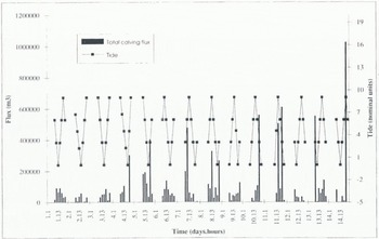
Fig. 11. The total calving flux observed from the north side during period 1 plotted against tidal stage. The calving observations and tidal stages relate only to daylight hours.

Fig. 12. The calving flux contributed by “large” and “extreme” submarine events observed from the north side during period 1 plotted against tidal stage. The calving observations and tidal stages relate only to daylight hours.
Discussion
Controls on the variability of calving activity
Few studies similar to this one have been undertaken. An early attempt was made in 1933 at South Crillon Glacier. Alaska (Reference Washburn,Washburn, 1936; Reference Goldthwait,, McKellar, and Cronk,Goldthwait and others, 1963). All calving into Crillon Lake was qualitatively monitored. Icebergs from above the waterline arcounted for nearly half the total “discharge”, although it is not clear whether this refers to frequency or flux. At least half the daily activity occurred in the quarter of the day around sunset with secondary peaks around midnight and at first light. No comparable diurnal pattern of activity is found in the present study. For South Crillon Glacier, surface velocity variations correlated closely with the weather, flow being fastest on sunny days and slowest during a cold rainstorm (Reference Washburn, and R,Washburn and Guldthwait, 1937), but no observations were made of the influence of weather on calving behaviour.
Recent observations of calving activity at several glaciers in Alaska have failed to yield any consistent patterns or significant correlations with environmental variables or particular crevasse patterns (personal communication from M.F.Meier, 1993). Between June and October 1983. A Post carried out a similar study to this one at Columbia Glacier, Alaska, and came to the same conclusion, namely that no straightforward relationships exist (personal communication from A. Post, 1993). At Glaciar San Rafael, most calving is apparently uncorrelated with any one variable, although the simple statistical analysis may fail to identify some of the natural relationships. A correlation between increased rainfall and accelerated calving, for example, has been demonstrated elsewhere for periods of less than 1 a (Sikonia and Post, 1980; Reference Theakstorne, and Knudsen,Theakstone and Knudsen, 1986), but in this study there was only a weak relationship. This discrepancy may reflect the incompleteness of the precipitation data and the absence of night-time observations.
Wave action can be ruled out as an important factor at Glaciar San Rafael because, even during storms with strong winds, wave action in Laguna San Rafael is damped to insignificant levels by the profusion of icebergs and brash ice. Wave action cannot he a necessary condition for rapid calving because two of the most actively calving glaciers in the world, Jakobshavns Isbæ, West Greenland, and Columbia Glacier, Alaska, calve into fjords so choked with floating ice that waves are insignificant Wind may have an indirect influence by controlling the turbulent-heat flux to the glacier, thereby surface ablation rates and hence meltwater discharge. On other Patagonian outlet glaciers, turbulent-heat transfer has been found to correlate closely with daily ablation variations (Reference Kobayashi,, Saito, and Nakajima,Kobayashi and Saito, 1985; Reference Ohata,, H,, H, and Nakajima,Ohata and others, 1985)
Calving activity is focused around the middle of the glacier and associated with high centre-line ice velocities, deep water, and foci of subglacial meltwater discharge. These are expected results. The observed relationship between calving and crevassing agrees with previous studies which have shown that crevasses carried to the ice front by glacier flow constitute the lines of weakness along which mechanical failure occurs (Reference Powell, and Molnia,Powell, 1983, Reference Powell, and Molnia,1991; Reference Epprecht,Epprecht, 1987, Reference Dowdeswell,Dowdeswell, 1989). Rapid and increassing velocities towards the front produce high extensional strain rates and stress weakening of the ice. Crevasse formation and calving are intimately linked problems, pointing again to the significance of strain rates.
The suggestion of a relationship, albeit a weak one, between tidal stage and calving flux conflicts with previous studies which have found no relationship between tide and calving (Reference Meier,Meier and others, 1980; Reference Brown,, Meier, and Post,Brown and others, 1982; Reference Qamar,Qamar, 1988) Changes in stress fields at the terminus associated with a tidal range of 1–2 m on an ice front over 300 m thick will not he great, but if stresses are already close to some critical threshold they may be enough to affect the timing of large events. At Columbia Glacier, maxima and minima of surface velocities correspond to low and high tides, respectively (Reference Walters,Walters, 1989), and it may he through this that tidal stage can indirectly affect calving activity. Buoyancy forces and back-pressure increase with rising tide while glacier velocities may increase at low tide, although Reference Laumann, and B,Laumann and Wold (1992) found that velocity maxima coincided with high-water stages. The effect on calving patterns of these opposing forces, and whether the relationships are constant, remains unclear.
Submarine calving
The observation that the largest bergs rise from below the waterline conforms with many similar observations of retreating temperate calving glaciers in Alaska (personal communication from A. Post, 1993).The disproportionate percentage of the total calving flux contributed by submarine calving (27% from 7% of the events) demonstrates the importance of this calving mechanism but raises an interesting question. About two-thirds of the total ice front is submerged, yet only a quarter of the calving flux consists of submarine bergs. The submarine and subaerial parts of the ice cliff presumably calve at much the same rate, so there is a conservation-of-mass problem. Given a calving front 3000 m long and 50 m high, the subaerial calving flux of 1.6 Mm 3 d−1 equates to a calving speed of 10.7 m d−1. The mean height of the submerged part of the cliff is 140 m, so the submarine flux of 0.58 Mm3 d−1 yields a calving rate of 1.4 m d−1. Calculations for only the north side yield subaerial and submarine calving speeds of 15.0 and 1.6 m d−1, respectively.
Part of these large disparities may be accounted for by differential flow within the glacier (due to basal drag), more rapid melting below the waterline and perhaps systematic underestimation of the size of submarine events. None of these factors, however, is likely to explain more than a small part of the difference. Abundant meltwater and presumed rapid sliding must minimize the differential between surface and basal-flow velocities. Melting is an equally unlikely explanation of the discrepancy because melt rates are typically insignificant relative to calving rates at the front (Reference Syvitski, and A,Syvitski, 1989; Reference Dowdeswell,, Murray,, Dowdeswelt, and Scourse,Dowdeswell and Murray, 1990). The present results suggest that, at this site at least, melt rates below the waterline are considerably greater than predicted by theory. Reference Powell, and Molnia,Powell (1983) too has recognized that melt rates at some glaciers must be high, and it may he that Equation (2) underestimates melt rates at temperate calving termini. Observational error is also an improbable explanation for the discrepancy; given that calved blocks break up less during submarine calving than during subaerial calving, submarine calving rates are more likely to he overestimated than underestimated.
The submarine-calving observations support the theoretical work of Reference Hughes,Hughes (1989) and Reference Hughes, and Nakagawa,Hughes and Nakagawa (1989) who reasoned that if the critical fracture stress at which calving occurs is the same above and below the waterline, submarine blocks will tend to be much larger than subaerially calved blocks. The contrast between shattered ice in the exposed cliff and more homogeneous submerged ice will contribute to this effect. Observatoions in Alaska using a remotely operated submersible have confirmed this contrast (personal communication from R. Powell, 1994).
However, these data contradict the more recent ideas of Reference Hughes,Hughes (1992). His suggestion of the relationship between the “calving ratio” and the “buoyancy ratio” implies that as a glacier approaches flotation the size of calved blocks is reduced. Field observations in Alaska (personal communication from A. Post, 1993) and at other Patagonian glaciers (Reference Warren,Warren, in press; Reference Warren,, Glasser, and Greene,Warren and others, in press a) all show that berg size is in part related to water depth, with larger bergs typically produced in deeper water.
The issue of the geometry of the submerged part of the ice cliff remains unresolved. No direct observation has the existence of a projecting underwater ramp. None of the investigations of Alaskan glaciers by Reference Meier,Meier and others (1980) revealed evidence of ice extensions at depth, although large bergs have been observed to emerge far in advance of the calving front at Columbia Glacier (personal communication from M. Meier, 1993). Reference Powell,Powell (1988b, p. 39) notes that “ice feet” can occasionally occur. At Glaciar San Rafael, the large submarine icebergs’ rising to the surface as much as 150 m beyond the ice cliff, their emergence vertically without any horizontal component of movement and the observations of subaerial events triggering submarine calvings all argue for the existence of a submarine “ice foot”. Reference Harrison,Harrison (1992) also infers a submarine “ice shelf”. A. Post (personal communication, 1993) argues that an “ice foot” can only exist during drastic retreat, but L. Hunter (personal communication, 1992) has observed frequent submarine calving associated with profuse subaerial calving at the front of the advancing Johns Hopkins Glacier, Alaska. It may be that the important factor is not advance or retreat but longitudinal strain rates, that where extensional strain is great and crevassing is intense, an enhanced contrast between shattered surface ice and more homogeneous bottom ice promotes the formation of an “ice foot”.
Calving speeds in tide water and fresh water
The salinity of Laguna San Rafael is only half that of the open ocean. The calving speed might therefore be expected to be intermediate between tide-water and fresh-water values. Reference Funk, and öthlisberger,Funk and Röthlisberger (1989) presented evidence that, for any given water depth, calving speeds in fresh water are about an order of magnitude smaller than those in tide water. Subsequent studies of fresh-water calving rates in Greenland (Reference Funk, and Haeberli,Funk and Haeberli, 1990), Norway (Reference Laumann, and B,Laumann and Wold, 1992) and Patagonia (Reference Warren,Warren, in press; Reference Warren,, Glasser, and Greene,Warren and others, in press a) have confirmed and refined this empirical relationship. That the calving speed of Glaciar San Rafael exceeds that predicted for tide water argues against a water-chemistry explanation for the contrast between calving rates in fresh water and tide water. Reference Funk, and öthlisberger,Funk and Röthlisberger (1989) appealed to the greater buoyancy of meltwater in tide water to explain the difference between fresh-water and tide-water calving rates, an explanation that requires a strong feed-back from melting to calving. The evidence for rapid melting in conjunction with high calving speeds at Glaciar San Rafael supports their proposed linkage.
Methodology
The methods used in this study have inherent weaknesses and provide only a partial record. Two quantitative methods exist which provide the potential for continuous monitoring of calving activity. Wave recorders and pressure transducers can detect calving events because of the distinctive wavelength of calving waves, and because wave amplitude is related to the net potential energy of the event (Reference Syvitski, and A,Syvitski, 1989). A pressure transducer was used successfully to record calving activity at Columbia Glacier, Alaska, in 1973 (personal communication from A. Post, 1993). Secondly, calving events produce relatively large-amplitude, low-frequency seismic signals (Reference Qamar,Qamar, 1988). Comparison of the results presented here and a simultaneous seismic record from a station on the north shore of the lagoon 2.5 km from the glacier (personal communication from R. Murdie, 1992) shows that much of the calving activity was detected. Such approaches can provide continuous, quantitative estimates of calving, but both require calibration using observational records. Furthermore, wave records are complicated by variable amounts of floating ice which damp wave crerts and affect wave direction. Neither method can detect small events unambiguously, differentiate between submarine and subaerial calving, or provide the kind of illuminating descriptive information about the nature of the events provided by observational records. Combinations of all these approaches could improve the accuracy of future calving studies.
Conclusions
Continuous monitoring of calving at Glaciar San Rafael has re-emphasized the great complexity of calving dynamics. It has shown that neither the fluctuations in the frequency of events nor the patterns of calving flux relate simply to single environmental variables. The only exception to this is the possibility that tidal stage has some influence on calving flux, particularly on the timing of major peaks in submarine calving activity. The largest bergs were produced by submarine calving, and bergs from the submerged parts of the ice cliff were typically larger than subaerially calved bergs. The distance from the front at which some of these bergs emerged suggests that there may be a projecting underwater “ice foot”. While contributing only a small number of total events, submarine calving produced over a quarter of the total recorded flux. Given that over two-thirds of the ice front is submerged, this figure indicates either that there is a pronounced deceleration down the vertical velocity profile, which is unlikely, or that melt rates below the waterline are considerably faster than theory predicts, or a combination of these.
The calving speed of about 4500 m a −1 in a mean water depth of 140 m adds further weight to the widely applied empirical relationship between calving speed and water depth developed by Reference Brown,, Meier, and Post,Brown and others (1982). However, that this calving speed is sustained in brackish water when it is known that calving speeds in fresh water are about an order of magnitude lower than those in tide water (Reference Funk, and öthlisberger,Funk and Röthlisberger, 1989) is surprising and suggests that some factor other than water chemistry explains the contrast. Although the physics of the water-relationship remain obscure, it has emerged as a robust and useful predictive tool that applies in a wide range of environments.
Acknowledgements
This research was carried out with the kind permission of CONAF (the Chilean Forest Service) in Coyhaique. Many thanks are due to the staff of Raleigh International (formerly Operation Raleigh), especially J. Cook and S. Belbin; in particular, the work would not have been possible without the enthusiasm and resilience of numerous Raleigh “Venturers”. C.R.W. was in receipt of a U.K. Natural Environment Research Council (NERC) Research Fellowship. S.H. and V.W.would like to thank the Royal Society Overseas Research Fund, the Percy Sladen Memorial Fund and Geotronics. A.R.K. was in receipt of a NERC Studentship. D. Sugden made helpful comments on an early draft. A. Post kindly shared insights from his many years of experience with Alaskan calving glaciers, and a thoughtful and searching review by R. LeB. Hooke substantially improved the manuscript. Detailed comments by R. D. Powell and an anonymous referee were also much appreciated.


