


1. Introduction
Surface melting shares considerably in the mass balance of the Greenland ice sheet (Reference BauerBauer, 1955; Reference WeidickWeidick, 1975; Reference Radok, Radok, Barry, Jenssen, Keen, Kiladis and McInnesRadok and others, 1982), which therefore reacts very sensitively to fluctuations in climate (Reference AmbachAmbach, 1980). Heat-balance data therefore provide a deeper insight into the relations between climatic disturbances and changes of the mass balance.
Kuhn’s concept allows the shift of the equilibrium line to be calculated in correlation to small climatic changes [Reference KuhnKuhn, 1981]. The algorithm proposed involves parameters which can be determined from heat and mass balance studies. The algorithm has already been applied to positions of the equilibrium line in the Alps and in the Andes (Reference KuhnKuhn, 1980, [Reference Quervain1982]).
During the International Glaciological Greenland Expedition (EGIG 1959 and 1967) detailed heat and mass balance studies were carried out in the area of ablation and accumulation (Reference AmbachAmbach, 1963, Reference Ambach1977[a], Reference Ambach[b]; Reference Ambach and MarklAmbach and Markl, 1983). In the present paper, results on Kuhn’s algorithm are discussed in order to estimate the response of the equilibrium line at the EGIG profile to small climatic disturbances.
The following are investigated in detail:
-
(i) the response of the net radiation balance to changes in air temperature, cloudiness, and albedo,
-
(ii) the response of the sensible heat flux to changes of the air temperature,
-
(iii) the altitudinal gradients of the air temperature and of the cumulative accumulation,
-
(iv) the duration of the ablation season, and
-
(v) the significance of the formation of superimposed ice.
The intention of the present paper is to analyse heat balance data measured at the EGIG profile for modelling according to Kuhn’s algorithm.
2. Radiation Fluxes
In connection with Kuhn’s concept, the following relations are examined
-
(i) The numerical relation between changes in air temperature and changes in long-wave downward radiation. In this connection, results of measurements of long-wave radiation balance have been evaluated as a function of cloudiness (section 2.1).
-
(ii) The dependence of the net radiation balance on the cloudiness and on the albedo. Results of measurements on snow surfaces and ice surfaces are used for this analysis (section 2.2).
2.1 Dependence of long-wave radiation balance on cloudiness
The dependence of the long-wave radiation balance on the cloudiness is used for calculating the relative emissivity of the atmosphere according to the Stefan-Boltzmann law. The long-wave downward radiation is given as
where ε+(w) is the relative emissivity at cloudiness w, σ is the Stefan-Boltzmann constant, and Ta is the actual air temperature valid for a representative radiation level. ε+(w) may be calculated as a function of cloudiness. Equation (1) gives a relation between temperature and long-wave downward radiation which is of significance for Kuhn’s algorithm.
The mean values of long-wave radiation balance LB as dependent on the cloudiness w for the series measured during EGIG 1959 and EGIG 1967 may be represented approximately by the following functions (Reference AmbachAmbach, 1963, p. 70, fig. 20; Reference Ambach and MarklAmbach and Markl, 1983, p. 28, fig. 11):


From, these results a relative emissivity of the atmosphere ε+(w) is calculated
where ε+(w) is a function of cloudiness. Assuming ε+(w) (10/10) = 1 and ε = 1 for the surface (To), we obtain

Furthermore, a melting surface may be assumed for the ablation season so that the numerical values of ε+(w) can be calculated from the series measured in EGIG 1959 (Reference AmbachAmbach, 1963, p. 70, fig. 20). A mean cloudiness of w = 5/10 is assumed. According to Equation (2a), LB (5/10) = −3.30 MJ m−2 d−1 and LB(10/10) = 1.20 MJ m−2 d−1. With σTo 4 = 4.90×10−3×273.154 = 27.3 MJ m−2 d−1 the value of 0.92 is thus obtained for ε+(5/10) according to Equation (3). An analogous evaluation of the EGIG 1967 series is not possible as the surface temperature cannot be assumed to be constant at the melting point.
The effect of an atmospheric temperature change δTa on the long-wave downward radiation δA may be calculated by the linearization

where α′ = 0.37 MJ/m2d K holds for ε+ (5/10) = 0.92 and 4σT0 3 = 0.40 MJ m−2 d−1 K−1.
It follows that
Equation (5) expresses the relation between a temperature disturbance δTa and a change in long-wave downward radiation δA.
2.2 Dependence of the net radiation balance on cloudiness
The dependence of the net radiation balance on the cloudiness is mainly governed by the albedo. This means that periods of different albedo must be examined separately (Table I). The differences in net radiation balance between a cloudiness of 0/10 and 10/10, however, can be formulated as a function of albedo only if the short-wave incoming radiation is nearly constant during the whole period of measurement. This holds approximately for the series measured in EGIG 1959 and in EGIG 1967, because the measurement periods are about symmetrical to the summer sols-tice. In an earlier paper it has been shown that a high albedo causes the daily sum of net radiation balance to increase as the cloudiness increases (Reference AmbachAmbach, 1974). This effect is explained by the fact that the fluctuations in net radiation balance at high albedo due to the dependence on cloudiness are governed by the fluctuations in long-wave radiation balance. Short-wave radiation balance here plays a minor role. This phenomenon, typical of polar regions, is of great interest and has already been discussed in detail (Reference AmbachAmbach, 1977[a] p. 31, fig. 15).
Table I. Daily mean values of Net Radiation Balance for Clear Sky and Covered Sky for various Albedo Values (Reference AmbachAmbach, 1977[a], p. 22, Table 5; Reference Ambach and MarklAmbach and Markl, 1983, p. 28)

Figure 1 shows the difference in net radiation balance NB(10/10) - NB(10/10) to be positive at low albedo and negative at high albedo. At a ≈ 0.66, the difference is zero. If the relation between the net radiation balance NB and the cloudiness w is expressed as
the following characteristic values β are obtained for different values of the albedo a from Table I and Figure 1: for dry snow surfaces (EGIG 1967):

for melting old snow surfaces:
for ice surfaces (EGIG 1959):

In order to specify the albedo at the equilibrium line during the ablation season, we must take into account that the surface layer may be a melting old snow layer or alternatively a melting superimposed ice layer. Melt water coming from an old snow layer here in general is completely trapped as superimposed ice which will melt again in the course of the ablation period. According to section 4.2 the duration of ablation from an old snow surface and that from a superimposed ice layer have the ratio of 2:1 yielding a weighted mean value B with β = 0 for melting old

The numerical correlation between changes in cloudiness δw(1/10) and in net radiation balance δNB is given by Equation (6):
Equation (8) can be used for calculating the effect of a change in cloudiness on the net radiation balance averaged over the ablation season at the equilibrium line.
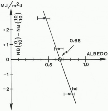
Fig. 1. Difference in net radiation for clear sky and covered sky plotted against albedo. Bars give the estimated range of variations in albedo. Values taken from Reference AmbachAmbach (1977[a], p. 22, table 5) and Reference Ambach and MarklAmbach and Markl (1983, p. 29, fig. 12).
3. Sensible Heat Flux and Heat Transfer Coefficient
The sensible heat flux Hs is frequently expressed by using the heat transfer coefficient α :
where Ta and To are the mean air temperature and the surface temperature respectively. Comparison of this expression with Prandtl’s formula for adiabatic layering shows α to be proportional to the shear velocity, and thus dependent on the wind velocity and the roughness parameter. This shows that α is not a micro-climatological constant.
For a period of 38 d, the sensible heat flux Hs was calculated for a melting ice surface, using Prandtl’s formula and allowing for the non-adiabatic layering (series measured in EGIG 1959). A mean value of Hs = 3.1 MJ m−2 d−1 (Reference AmbachAmbach, 1977[a], p. 41, table 9b) is obtained with the roughness parameter z = 2.21×10⁻³m and the shear velocity ux = 0.44 m s−1 (Reference AmbachȦmbach, 1977[b], p. 17, fig. 5b). Both quantities were obtained from the logarithmic wind profile (Fig. 2). The mean value of the air temperature at 187 cm altitude is 1.8°C in the ablation period under observation (Reference AmbachAmbach, 1977[a], p. 41, table 9b). With To = 0°C, Ta = 1.8°C, and Hs = 3.1 MJ m−2 d−1, α is calculated from Equation (9) to be 1.72 MJ m−2 d−1 K−1 which agrees with the value reported by Reference KuhnKuhn (1979).
The heat transfer coefficient for a snow surface must be calculated separately owing to the different roughness parameter. Under otherwise equal conditions, with different shear velocities, the relation

is valid. Hence

with u+(snow) = 0.276 m s−1, u+ (ice) = 0.440 m s−1 (Fig. 2) and α (ice) = 1.72 MJ m−2 d−1 K−1, we obtain the heat transfer coefficients = 1.08 MJ m−2 d−1 K−1 characteristic of a snow surface. Precisely, this value is valid only for a wind velocity of u = 7 m s−1, 2 m above ground, as was measured in this series (expressed in round numbers, cf. Reference AmbachAmbach, 1977[b], p. 16, fig. 3).

Fig. 2. Mean wind profiles for the entire duration of measurements
(a) EGIG 1959, mainly ice surface
(b) EGIG 1967, snow surface only
according to Reference AmbachAmbach (1977[b], p. 17, fig. 5).

Fig. 5. Formation of superimposed ice in a schematic diagram. Q = heat (MJ m−2), m = water equivalent (kg m−2), h = depth (m), τ = number of days
(a) without formation of superimposed ice
(b) with full formation of superimposed ice.
According to section 4.2, for two-thirds of the ablation period at the equilibrium line there will be an old snow surface, and for one-third of the time the surface will be superimposed ice. The sensible heat flux under these assumptions may thus be expressed by a weighted mean value α, covering the total ablation season

Equation (9) and To = 0°C therefore yield the following relation between change of the sensible heat flux δHs and the change in air temperature δTa:
Equation (13) permits calculation of the change in sensible heat flux caused by a variation in temperature at the equilibrium line.
4. Heat Balance
4.1 Heat balance of snow and ice surfaces
The balance equation takes the following form, positive terms being energy sources, negative terms being energy sinks
where the terms represent the net radiation balance, the flux of sensible heat, the flux of latent heat, the heat of conduction, and the heat of melt.
The series of measurements from EGIG 1967 gives the heat balance for a prevailingly dry snow surface from 15 May to 27 July 1967. The mean value of albedo over the entire period of measurement is 0.85 for an undisturbed surface. Traces of melting were observed only on eight days. The albedo on these days dropped to a minimum of 0.73 (Reference Ambach and MarklAmbach and Markl, 1983, p. 22, fig.5).
Table II lists the mean values of the heat balance components for the whole period of measurement. Theoretically, the balance figure must be zero (instead of +0.3 MJ m−2 d−1). This discrepancy is due to errors of measurement. The error is < 1% in relation to the sum of energy sources.
Table II. Mean Values of the components of the Heat Balance (MJ m−2 d−1), 15 May—27 July 1967 (7 d, EGIG 1967, Albedo = 0.85, Wind Velocity: ū (2 m) = 7 m s−1, Air Temperature: T(2m) = −6.3°C, Vapour Pressure: ē (2m) = 3.2 mbar, Cloudiness: w = 4.7/10 (Reference Ambach and MarklAmbach and Markl, 1983, p. 61, table 11b)

The EGIG 1959 series of measurement is characterized by strongly changing albedo, since the surface changed from new snow to old snow and ice. It is therefore meaningful that the components should be given in sections covering periods with characteristic surfaces (Table III). The balance sum yields the theoretical value zero, HM being determined from the balance equation. For control see Reference AmbachAmbach (1977[a], p. 41-42, table 9). Furthermore, graphical comparisons have been made for the sections with snow and ice surfaces respectively as regards the following components: SB, LB, HS, HL, Hc and HM (Fig. 3). Snow surfaces receive much less heat for melting than ice surfaces. The energy HC consumed in heating ice is about 1 MJ m−1 d−1 changing only slowly during the entire period. The fluxes of sensible heat and latent heat (Hs, HL) show considerable fluctuations owing to changing microclimatological conditions, the amounts, however, being only of secondary importance for the melting energy. The essential component is the shortwave radiation balance SB, which shows a correlation with the melting energy HM.

Fig. 3. Components of heat balance given for various periods (cf. Table IV). SB = short-wave radiation balance, LB = long-wave radiation balance, HS = sensible heat flux, HL = latent heat flux, HC = conductive heat flux, HM = heat of melting.
Table III. Mean Values of the components of Heat Balance (MJ m−1 d−1) for various Surfaces, EGIG 1959 (Reference Ambach and MarklAmbach and Markl, 1977[a], p. 41, table 9a-c)

For studying the relation between SB and HM, a graph was made for six sub-periods with HM as a function of SB (Fig. 4). In addition, Figure 4 shows the value of SB plotted for HM = 0 for the period of EGIG 1967 (period 7, Table IV). The relation between SB and HM according to Figure 4 can be characterized as fol1ows:
The relation may be approximated by a straight line independent of the situation (snow surface or ice surface). The straight line runs partially outside the error limit, which for each radiation flux, short-wave incoming and short-wave reflected radiation, has been assumed to lie within 2%. This means that the sum of LB + HS + HL + HC determined by micrometeorological quantities, is only approximately constant. Period 5 does not comply with this requirement. In this case, very strong evaporation is combined with a strong negative value of long-wave radiation balance.
The slope of regression line is ∆Hm/∆SB = 1.11. If the slope were unity this would mean that changes in SB were equivalent to changes in HM.
The correlation between SB and HM corresponds to a threshold function, the threshold being SB+ = 4.5 MJ m−2 d−1; a value which can be taken from Figure 4 as being the point of intersection with the SB axis. For SB ⩽ SB+, the amount of SB is used for compensating the energy sink LB + Hs + HL + HC. For values of SB > SB+, the difference ∆SB = SB - SB+ is used entirely for melting.
This result is of significance in so far as ice or snow ablation by melting may be approximately determined from the easily measured quantity SB, also useful for estimating ablation for specific sites. This simple method can be applied only if the sum SB + HS + HL + HC is approximately constant, the threshold SB+ being known. In periods of extremely low or high cloudiness, or if the micrometeorological quantities are extreme, this numerical condition is not satisfied (cf. period 5, Fig. 4).
The value of ∆HM/∆SB = 1.11 furthermore indicates that higher SB values in general mean additional energy for melting is available. The energy for melting provided by ∆SB is increased by other energy sources by about 11%. This difference may be allowed for by reducing the energy sinks by 11%.
For further discussion, the threshold function is divided into the regions 1 and II (Fig. 4). In the ablation period with strong ice or snow melting, the energy balance satisfies the conditions of region II, i.e. the short-wave radiation balance SB is partly used for compensating the energy sink LB + Hs + HL + HC and partly used for energy of melting HM. At the end of the ablation period we reach a situation when SB = SB+. As the season progresses further, SB still decreases in region I. As there is no melting in region I, the point of state shifts along the SB axis towards zero. In this region, the energy balance is valid in the form of SB + LB + Hs + HL + HC = 0, with SB < SB+. If zero is reached in the polar night (SB = 0), energy sources and energy sinks compensate without any contribution from the short-wave radiation balance, the energy balance being LB + HS + HL + HC = 0.
Table IV. Micrometeorological Data for specific periods, data referring to Fig. 4 (Reference AmbachAmbach 1977[a] p. 41, table 9a; p. 45, table 13a-e; Reference Ambach and MarklAmbach and Markl, 1983, p. 58, table 8)


Fig. 4. Heat of melting (HM) versus short-wave radiation balance (SB) for seven periods (cf. Table IV). I = range without any melting, II = range with melting. The bars give the error limits for SB.
4.2 Formation of superimposed ice
In the region near the equilibrium line, the formation of superimposed ice is of decisive importance for mass balance and for energy balance (Reference AmbachAmbach, 1963; de Reference QuervainQuervain, 1969). Superimposed ice forms from melt water coming from the old snow layer and collecting at the impermeable cold ice surface where it freezes. The heat of melting liberated is thus conducted into the underlying ice. The energy transformation under the condition of total formation of superimposed ice is shown in Figure 5b. Q0 is the energy per unit area required to melt the old snow layer h0 with no superimposed ice forming (Fig. 5a), Q1 + Q2 is the energy per unit area necessary for melting the old snow layer h1 plus the superimposed ice layer h2. Q1+ Q2 > Q0 is valid since the temperature of the ice body rises as the formation of superimposed ice progresses. This energy must be expended additionally. The liberated heat of melting and the energy used for heating the ice by heat conduction are equal. If the total melt water from the old snow layer is consolidated as superimposed ice, then Q0 = Q2 and Q1 = Q3 (Fig. 5b).
Superimposed ice formation has been calculated repeatedly for different initial and boundary conditions (Reference AmbachAmbach 1963; Reference Quervainde Quervain 1969). With representative values of the initial temperature (−10°C) and of the temperature gradient in the depth profile (1 K/m), 0.4 to 1.4 cm of superimposed ice per day will form during the ablation period (Reference AmbachAmbach, 1963, p. 169, fig. 68).
The formation of superimposed ice leads to a change from a melting old snow surface to a surface of melting superimposed ice during the ablation season. This situation has a marked effect on the energy balance, as the albedo and the roughness parameter are changed considerably by that fact.
In the region of stake BK 7 (1241 m a.s.l.) lying approximately at the equilibrium line, all the melt water from the old snow presumably turns into superimposed ice. The minimum snow temperature there (−8°C) was measured before the ablation season set in (Reference AmbachAmbach, 1963, p. 160, fig. 64), the minimum ice temperature at 2 m depth under the ice surface being −10°C. The snow density in the vertical profile was between 300 and 400 kg/m3.
Before describing the effects which the superimposed ice has on the energy balance during the ablation season, the duration of the intervals with a snow surface and an ice surface must be known. The calculation is made as follows, the density of old snow ρ1 = 300 kg/m3 and that of superimposed ice ρ2 = 900 kg/m3. Index 1 refers to the old snow layer and index 2 refers to the newly formed superimposed ice layer (Fig. 5b).
Maximum thickness of the superimposed ice:
For the maximum thickness of the superimposed ice layer h2, that may form from the old snow layer h0, the following equations are obtained from the conservation of the total mass:


Heat of melt:
Transformation of the old snow layer h1 into a superimposed ice layer h2 and subsequent melting requires energy as follows (Fig. 5b):


Duration of ablation of old snow surface τ1 and of superimposed ice surface τ2:
For calculating the number of ablation days with a snow surface and with an ice surface it is necessary to know the energy balance for both surfaces. Thus

where HM(1) and HM(2) are the heat of melting per day per unit area resulting from the energy balance, the index (1) being valid for a snow surface and the index (2) for an ice surface.
The numerical difference between Hm(1) and HM(Z) is due to the change in albedo and in roughness parameter resulting from the transition from a snow surface to an ice surface. From the energy balance we obtain the following equation for the heat required for melting (Equation (14):
where NB, HS, HL, and HC are the net radiation balance, the sensible heat flux, the latent heat flux, and the conductive heat flux into the ice. For a non-melting surface HM = 0.
Transition of a dry snow surface into the state of melting (1), or into a state of melting of a superimposed ice layer (2), yields the daily energy output HM(1), HM(2) as the difference values ∆HM(1), ∆HM(2) from
where ΔNB means the change in net radiation balance due to the change in albedo, ∆(HS + HL) is the change in sensible and latent heat fluxes due to changes of the roughness parameter, and ∆HC, the change of the heat conduction in ice, which depends on the change in temperature gradient. If we assume that changes in the albedo ∆a are of predominant importance in causing changes in the heat of melting ∆HM, we obtain the following approximation averaged over the ablation period
For a transition from a dry surface to a melting surface we have ∆HM = HM. For ∆a1 = 0.15 and ∆a2 = 0.45 it follows that

Here, with the onset of melting, the albedo of the dry snow surface was assumed to decrease from 0.85 to 0.70 (∆a1 = 0.15) and for a superimposed ice surface it was assumed to decrease from 0.85 to 0.40 (∆a2 = 0.45). Equation (23) approximately agrees with the result of section 4.1, Figure 4, where
is well satisfied for ∆G = 0.
For Equation (19) we thus have

The ablation period of the superimposed ice layer іs therefore 50% shorter than that of the old snow-pack. This difference is due to the low albedo of the ice surface as compared to the snow surface, and is valid even though the mass of the superimposed ice layer is 50% higher than that of the melted old snow layer (Equation (16)). In an ablation season of 30 d, for example, the old snow surface will exist for 20 d, while an ice surface exists for only 10 d.
4.3 Duration of the ablation season
If days having a mean temperature of T ≥ 0°C are said to be ablation days, their number in the ablation season may be calculated as a function of altitude. This calculation is based on temperature values from the meteorological station on the west coast (Jakobshavn station, 40 m a.s.1.) and on the temperature gradient in the EGIG profile. Comparison of temperatures from the Jakobshavn station and those from station Camp IV EGIG 1959 during the ablation season 1959 yielded a temperature gradient of 0.73 K/100 m (Reference AmbachAmbach, 1977[a], p. 36, fig. 19). Reference BraithwaiteBraithwaite (unpublished) pointed out that large glacier regions show horizontal gradients in addition to the vertical gradient > 0.6 K/100 m. From the meteorological records of Jakobshavn station, the number of ablation days as dependent on the altitude were newly calculated for the years 1958 to 1971 (Fig. 6). The resulting minimum, mean, and maximum durations of the ablation season at 500 m, 1000 m (Camp IV-EGIG 1959), 1240 m (equilibrium line), 1500 m, and 1850 m (Carrefour-EGIG 1967) are listed in Table V for the indicated length of time. For the equilibrium line at an altitude of 1241 m a.s.l. (BK 7), 15-75 ablation days are obtained by interpolation, 35 ablation days being obtained from the mean curve. It must, however, be emphasized that the actual number of ablation days is higher than the number here calculated. The reason is that melting takes places at noon even if the air temperature has a daily mean value of T < 0°C. The values of ablation periods given in Figure 5 are to be taken as lower boundary values.

Fig. 6. Number of ablation days (T ≥ 0°C) versus altitude calculated from values of air temperature in Jakobshavn station (40 m a.s.l.) and an altitudinal gradient of air temperature of 0.0073 K/m.
Table V. Minimum, Mean, and Maximum durations of the ablation season at various altitudes taken from Figure 6 (Rounded Values)

The number of ablation days (T ≥ 0°C) for the series of measurements EGIG 1959 and EGIG 1967 may be taken directly from the 24 h mean values of air temperature and may be compared with the data taken from Table V. From air temperature measurement the following results are obtained:
for EGIG 1959, 16 May—8 August 1959 (Reference AmbachAmbach, 1963, p. 268, table 42): 45 ablation days (55 ablation days according to Fig. 6).
for EGIG 1967, 20 May—28 July 1967 (Reference AmbachAmbach, 1977[b], p. 20, table 3): 3 ablation days (5 ablation days according to Fig. 6).
The figures in parentheses are taken from the mean curve of Figure 6 for 1000 m a.s.l. (EGIG 1959) and for 1850 m a.s.l. (EGIG 1967). Statistical studies of temperature values at Jakobshavn station show that the years 1959 and 1967 correspond well with the mean values of the period 1958–1971 (Reference AmbachAmbach, 1977[a], p. 61, fig. 25). The difference of 10 ablation days for EGIG 1959 is understandable as the ablation season at sea-level need not have terminated at the end of the period of measurements (8 August 1969).
4.4 Winter accumulation
Depths of snow forming the winter accumulation from August 1958 to May 1959 at altitudes between 612 m a.s.l. (BK 1) and 1241 m a.s.l. (BK 7) were measured during EGIG 1959 (Reference AmbachAmbach, 1963, p. 298, table 53). Data were converted into water equivalents using the snow densities at the sites of measurement. In order to extrapolate the water equivalents for the whole balance year 1958/59, the water equivalents were multiplied by the factor of 12/9 = 4/3. Figure 7 shows the extrapolated values of the water equivalent plotted versus altitude, the gradient amounts to 0.55 kg m−2m−1 as being valid in the region below the equilibrium line. Using Kuhn’s algorithm in relation to superimposed ice, the effective gradient according to Equation (18) is

In the region above the equilibrium line, the gradient of accumulation can be found by pit studies at sites without any run-off. Such pit studies were carried out on the EGIG profile by Reference BensonBenson (1962) at altitudes above 1746 m a.s.l. and by de Reference QuervainQuervain (1969) at Camp VI-EGIG, 1684 m a.s.l., Carrefour 1850 m a.s.l., and Milcent 2448 m a.s.l. Regardless of the fact that the averaged rate of accumulation in pit studies can be obtained over a certain period, the values from those sites need not necessarily represent the condition at the equilibrium line. No accumulation data are available at altitudes between 1241 m a.s.l. (BK 7) and 1648 m a.s.l. (Camp VI-EGIG), which may be important for consideration of the shift of the equilibrium line in response to climatic warming.

Fig. 7. Winter accumulation in the ablation area measured between 7 and 20 May 1959 versus altitude. Measured values are extrapolated by the factor 12/9 = 4/3 for the balance year (cf. Reference AmbachAmbach, 1963, p. 298, table 53).
5. Conclusions
For applying Kuhn’s algorithm to the EGIG profile, special heat-balance quantities at the equilibrium line must be known. The equilibrium line may generally be assumed to be near 1241 m a.s.l. This altitude results from mass-balance measurements at the EGIG profile. In particular in 1959, at the end of the ablation season, it was found that bS = 0 at the site of BK 7 at 1241 m a.s.l. (Reference AmbachAmbach, 1963, p. 151, fig, 58a). The balance year 1959 represents average conditions with respect to the number of days with ablation (Reference AmbachAmbach, 1977[a], p. 61, fig. 25). At BK 7 superimposed ice showed maximum thickness and was found to have melted completely by the end of the ablation season. However, no ice from previous years was ablated.
In 1959 the water equivalent of winter accumulation at BK 7 amounts to 349 kg m−2, the snow depth being 0.85 m. The maximum thickness of 0.28 m of the superimposed ice layer results from Equation (15). The number of days with ablation was 35 d (Fig. 6 and Table V), consequently the interval during which there was a snow surface lasts for 23 d and that with a superimposed ice surface for 12 d (Equation (24)). The heat consumed for melting both the old snow and the superimposed ice layer results from Equation (18):

Consequently, a daily energy input of 5.6 MJ m−2 d−1 is obtained for melting averaged over the period of 35 d. At the equilibrium line, no heat-balance measurements were carried out during EGIG. Only data from the central ablation area at 1013 m a.s.l. (EGIG 1959) and from the accumulation area at 1850 m a.s.l. (EGIG 1967) are available. Results of EGIG 1967 are assumed to be representative for the dry snow surface without significant melting, those of EGIG 1959 for the melting ice surface. From both studies the proper heat-balance quantities at the equilibrium line are derived for Kuhn’s algorithm:
The quantity α (Equation (9)) depends on the shear velocity, which is influenced by the surface roughness and the wind velocity. The shear velocity for the ice surface is taken from EGIG 1959, that for the snow surface from EGIG 1967.
The quantity α′ (Equation (4)) depends on the surface temperature. The results of EGIG 1959 with surface temperatures at 0°C are applied for the whole ablation period at the equilibrium line.
The quantitity β (Equation (6)) depends significantly on the albedo. For a wet old snow surface (β ≈ 0, the albedo being 0.66 (Fig. 1). For an ice surface the value of β was taken from EGIG 1959.
At the equilibrium line the ratio of the number of days with a melting snow surface and with melting superimposed ice is 2:1 (Equation (24)). Consequently, the quantities which depend on the type of surface snow or ice (α, β), are averaged using the weights 2:1. The mean values are (Equations (7) and (12)):


The quantity α′ has the same value for snow and for ice surfaces. Therefore no weighted average need be calculated for this quantity.
The formation of superimposed ice influences significantly the amount of heat necessary for melting the winter accumulation (bS = 0). Comparing both conditions, superimposed ice and no superimposed ice, the ratio of the heat for melting the total winter accumulation amounts to 5/3 according to Equation (18).
Assuming Kuhn’s algorithm for the calculation of the shift of the equilibrium line (Reference KuhnKuhn, [1981]; Reference AmbachAmbach, in press)

with the conditions:
-
(Reference Reeh, Reeh, Clausen, Dansgaard, Gundestrup, Hammer and JohnsenReeh and Others, 1978)

-
Equation (27)
-
Equation (5)
-
Equation (28)
-
Equation (25)
-
Table V


and L = 0.3336 MJ kg−1, specific heat of melt, the shift becomes:


Discussions on the response of the equilibrium line to climatic disturbances are published elsewhere in detail (Reference AmbachAmbach, in press; Ambach and Kuhn, in press). Further effort is necessary to inititate heat-balance investigations in the other regions of the Greenland ice sheet in order to apply Kuhn’s algorithm for the entire Greenland ice sheet.
List of Symbols and Units


