


Introduction
The past two decades of study in West Antarctic ice sheet (WAIS) dynamics have revealed that the large ice streams draining Marie Byrd Land ice into the Ross Ice Shelf are responsible for the observed changes in the condition of the ice sheet (Reference Alley, Bindschadler, Alley and BindschadlerAlley and Bindschadler, 2001). Five major ice streams are involved, moving at speeds up to 700 ma–1. These high flow speeds are possible due to basal lubrication above and possibly within a subglacial layer of weak, water-saturated till (Reference Blankenship, Bentley, Rooney and AlleyBlankenship and others, 1986; Reference Alley, Blankenship, Bentley and RooneyAlley and others, 1987; Reference Kamb, Alley and BindschadlerKamb, 2001). Significant variations in ice-stream flow behavior would necessarily affect the inland ice sheet which, as a marine ice sheet, is potentially unstable (Reference MercerMercer, 1968; Reference WeertmanWeertman, 1974; Reference Alley, Bindschadler, Alley and BindschadlerAlley and Bindschadler, 2001).
Observations have revealed evidence that the ice streams constitute a complex dynamic system with large changes having occurred during the past several hundred years. For example, Whillans Ice Stream (WIS) is slowing down (Reference Bindschadler, Stephenson, Roberts, MacAyeal and LindstromStephenson and Bindschadler, 1988; Reference Bindschadler and VornbergerBindschadler and Vornberger, 1998; Reference Whillans, Bentley, van der Veen, Alley and BindschadlerWhillans and others, 2001; Reference Joughin and TulaczykJoughin and others, 2002), amplifying its positive mass balance (Reference Joughin and TulaczykJoughin and Tulaczyk, 2002). Kamb Ice Stream (formerly Ice Stream C) ceased flowing rapidly approximately 150 years ago (Reference Retzlaff and BentleyRetzlaff and Bentley, 1993; Reference Smith, Lord and BentleySmith and others, 2002), and one of its tributaries is shifting flow direction to feed WIS (Reference Price, Bindschadler, Hulbe and JoughinPrice and others, 2001; Reference Conway, Catania, Raymond, Scambos, Engelhardt and GadesConway and others, 2002). The existence of a relict ice stream which flowed across what is now the northeastern flank of Siple Dome was discovered (Reference Jacobel, Scambos, Raymond and GadesJacobel and others, 1996; Reference Gades, Raymond, Conway and JacobelGades and others, 2000), and determined to have stopped flowing rapidly about 450 years ago (Reference Jacobel, Scambos, Nereson and RaymondJacobel and others, 2000; personal communication from B.E. Smith, 2005).
To be important at larger spatial or temporal scales, direct measurements of changes in geometry and flow must be sustained. In this paper, we report recent changes in the mouth of WIS and discuss these changes in the context of other observations and analyses of this area by ourselves and others spanning more than 40 years. Examination of multiple parameters helps in determining functional relationships between parameters and provides clues to causal mechanisms of change.
History of Ice-Plain Observations
The region of interest is where WIS enters the Ross Ice Shelf, beginning where it meets Mercer Ice Stream (formerly Ice Stream A) to the south and ending at Crary Ice Rise to the northwest (see Fig. 1). This transitional area, a hybrid between an ice stream and an ice shelf, is called an ‘ice plain’ (Reference Alley, Blankenship, Rooney and BentleyAlley and others, 1989). It is characterized by low surface slopes, typically 10–3, and low basal stresses, typically 10–30 kPa (Reference BindschadlerBindschadler and others, 1987). Generally, this ice plain experiences lateral extension due to the widening of the stream and the flow diversion forced by the stagnant Crary Ice Rise which is blocking its path. Longitudinal compression also results from the encounter with Crary Ice Rise. Regionally smooth velocity variations exhibit minor local variations due to locally variable basal stress (Reference BindschadlerBindschadler, 1993).

Fig. 1 Location map of the study area, illustrating positions of the datasets summarized in Table 1. The 19 named ice-velocity stations are labeled in black (RIGGS era) and in white (SCP era). Ice-thickness data locations are depicted by various symbols (see legend). When two ice thicknesses are available for a location, the older is indicated. Three versions of the grounding line in the vicinity of the ice plain are shown in white: from airborne radar (dashed line; Reference Shabtaie and BentleyShabtaie and Bentley, 1987); interpreted from surface features seen in SPOT images (solid line; Reference BindschadlerBindschadler, 1993); and derived from SAR interferometry (dotted (smaller uncertainty) and dash-dot (larger uncertainty) lines; Reference GrayGray and others, 2002). Background image is the version 1 RAMP SAR image mosaic acquired in 1997 (Reference JezekJezek and others, 2002). Thirteen SPOT images are overlain and include some clouds (irregular bright patches) and cloud shadows (irregular dark patches). Acquisition of the optical imagery spans the 4 years 1988–92. Former ice stream names are shown below the current names. Ice flow is from upper left toward lower right.
The extended time series of observations of the Whillans ice plain is partly a fortunate consequence of its location. Once believed to be part of the southeastern Ross Ice Shelf, several early field groups traversed the region (see Reference Bentley, Hayes and BentleyBentley, 1984). The earliest were the Pole-bound explorations of Amundsen (in 1911–12), followed by Gould (in 1928) and Blackburn (in 1935). More detailed scientific expeditions to the area began with the International Geophysical Year (IGY; July 1957–December 1958) and included a 3 year long (1957–60) exploration and mapping circumtraverse of the Ross Ice Shelf (Reference Crary, Robinson, Bennett and BoydCrary and others, 1962). As a result of the IGY, the Ross Ice Shelf became one of the most investigated regions of Antarctica, yet the studies were still limited in spatial extent.
During the 1960s, the development of airborne radioecho sounding (RES) resulted in an improved map of ice- shelf thickness. Airborne radar sounding flights conducted during the mid-1970s provided the detail necessary to better define the ice streams of the Siple Coast (Reference RoseRose, 1979). They had previously been coarsely mapped from reconnaissance flights and aerial photographs, and the new results included elevation maps of the largely unknown subglacial bed.
Between 1973 and 1978, the Ross Ice Shelf Geophysical and Glaciological Survey (RIGGS) improved the state of knowledge about the ice shelf through a multifaceted effort. An extensive survey was conducted, with many measurements carried out at almost 200 remote stations We review geophysical data acquired by campaigns forming a grid that covered the entire ice shelf (Reference Bentley, Hayes and BentleyBentley, 1984). The Whillans ice plain, thought to be part of the floating ice shelf, was included in this survey.
During the 1980s, interest in the ice streams and their interaction with the Ross Ice Shelf grew into a program of coordinated glaciological and geophysical fieldwork, informally called the Siple Coast Project (SCP). Initially, SCP fieldwork concentrated on Whillans and Kamb Ice Streams (called B and C, respectively, during the SCP), with studies being carried out in their catchment areas, on their main trunks, on the interstream ridges, and in their mouths where discharge into the Ross Ice Shelf occurs. Later SCP studies revisited the mouth of WIS where new sites were interlaced with RIGGS stations from 10 years earlier, and included investigations on Crary Ice Rise itself.
The work has since expanded to include Bindschadler and MacAyeal Ice Streams (formerly Ice Streams D and E, respectively) and their catchment basins, as well as the interstream ridges and Siple Dome as part of the WAIS project. Coupled with airborne and ground-based observations, satellite remote sensing from a number of sensors has played an increasingly important role in change detection over the expanded area of interest. The remotely sensed observations and the impetus of directly measuring surface changes of the Whillans ice plain motivated a more recent set of field measurements of this region in 1999.
We review geophysical data acquired by campaigns associated with the IGY during the 1950s, RIGGS during the 1970s, SCP during the 1980s and WAIS during the 1990s. Satellite data sources are Système Probatoire pour l’Observation de la Terre (SPOT) and RADARSAT during the 1980s and 1990s. The observations used here and their associated errors are discussed next and are summarized in Table 1. Technological advances over the four decades spanned by our study are evident in the increased spatial coverage and greater measurement precision of the more recent data.
Table 1. Sources of data discussed in the text

Grounding-Line Measurements
The grounding line is defined as the boundary between grounded and floating ice. For WIS, this boundary has been determined multiple times from several sources over the past three decades. Most of these interpretations are shown in Figure 1 and listed in Table 1. A concise history of the grounding zone mapping is given by Reference GrayGray and others (2002); here we provide a brief review.
The earliest determination of the grounding line was derived from the 1974–75 Scott Polar Research Institute (SPRI)–Technical University of Denmark (TUD)–US National Science Foundation (NSF) airborne RES program. Grounded ice was identified where the surface elevation was higher than that for floating ice of the same thickness. The ice plain was at the edge of the flight grid, forcing extensive interpolation. The grounding line was constrained best only at the lateral ice-stream margins (see Reference RoseRose, 1979, fig. 1). Surface slope and measurement error combine for a grounding-line position error of ±2 km, and the flight navigation error is ±5 km. Its position is not shown in Figure 1, but it lies close to a flow-transverse line between sites B18, DNB and A19. This line roughly separates the steeper ice-stream ‘trunk’ from the shallower-sloped ice plain, a boundary Reference Alley, Blankenship, Bentley and RooneyAlley and others (1987) refer to as the ‘coupling line’.
During 1984/85, many more airborne radar sounding data of the ice plain were obtained by the University of Wisconsin’s Glaciogeophysical Survey of the Interior Ross Embayment (GSIRE; Reference Shabtaie and BentleyShabtaie and Bentley, 1987). These authors considered the character of the radar return and the presence of bottom crevasses in addition to computing the height above flotation. Their revised grounding-line position is approximately 70 km downstream of its position based on the earlier data (less at the ice-stream margins) and has a different shape. It is discontinuous in the region directly upstream of Crary Ice Rise, due to isolated local grounding and intense crevassing (see Reference Shabtaie and BentleyShabtaie and Bentley, 1987, fig. 12). The navigation of this data is superior to that of Reference RoseRose (1979) because the flights were tied to numerous ground stations with satellite geoceiver position fixes accurate to ±15 m or less. Local observations, including optical leveling to measure surface elevation profiles, visual identification of strand cracks, and tiltmeter observations (Reference BindschadlerBindschadler and others, 1987), agreed well with the grounding-line position determined by Shabtaie and Bentley.
SPOT satellite images provided another means of mapping the grounding line. Thirteen scenes collected between 1988 and 1992 cover much of the ice-plain area. This optical imagery shows an undulated ice surface, resulting from ice flowing across a non-uniform bed, distinct from floating ice with a smoother surface (Reference Jacobel, Robinson and BindschadlerJacobel and others, 1994). Reference BindschadlerBindschadler (1993) mapped the grounding line from this imagery. The positional error of the grounding line combines the geolocation error of the SPOT scenes, approximately ±1 km, and the subjective interpretation of the imagery that is estimated at <1 km.
Satellite radar interferometry of RADARSAT-1 Antarctic Mapping Project (RAMP) data acquired in 1997 was analyzed by Reference GrayGray and others (2002) to determine the grounding-line location by identifying where the phase of the returned radar pulses changed rapidly. While the uncertainty of the position varies, it is as small as ±1–2 km. The areas with larger uncertainty are identified in Figure 1 by a different texture line.
There is general agreement among the most recent three grounding-line estimates, all shown in Figure 1. Each includes a deep embayment of floating ice towards site M0 and incorporates Crary Ice Rise as a continuous part of the grounded ice plain. Details of the different estimates are related to the strengths and weaknesses of each method.
Grounding-Line Changes
Some of the differences between grounding lines shown in Figure 1 may express real change. If so, there is no uniform advance or retreat evident. Most of the difference is probably related to the different methods used to determine the grounding-line position. For example, the GSIRE estimate is best where flight-line coverage exists, whereas the synthetic aperture radar (SAR) method is more sensitive to areas where the tidal variation is greatest.
A second generation of SPOT images was acquired in January 1999 to search for changes in a grounding line determined by a consistent method. Six scenes were collected covering the downstream half of the ice plain (approximately between stations N1 and H10; see Fig. 2a). Separated by about 10 years, most of the grounded ice appeared not to have changed. The most obvious change in the sun-illuminated topography was in a small region just upstream of station E2.3A and near the IGY site ‘26.1’ (see Fig. 2a). The floating ice surrounding a previously isolated grounded patch had become grounded itself, joining the ice plain and advancing the grounding line at an average rate of 340m a–1. This is similar to the rates (discussed below) that were determined by comparing surface elevations.

Fig. 2 (a) Subset of image map of Figure 1 including velocity stations from SCP (white), RIGGS (black) and IGY stations 26.1 and 28.0 (black triangles). Grounding lines derived from imagery are shown in white for 1989 (solid line) and for 1999 (dotted line). Heavy black lines depict surface elevation profile locations. Those labeled with white circled numbers 1 and 2 are shown in (b). White stars indicate the older measured grounding-line position along those profiles (in 1958 for profile 1, and in 1984 for profile 2). White and black circles and squares are locations of specific ice- thickness comparisons discussed in the text. (b) Surface elevation along profiles 1 and 2 identified in (a). Vertical adjustments are discussed in the text. Older grounding-line locations from this figure are shown in (a) as white stars.
Surface Elevation
During the IGY Ross Ice Shelf traverse of 1957–58, surface elevation was measured at a variable spacing of 1–10 km, by barometric altimetry corrected for temporal pressure changes measured at fixed stations. Distribution of the 22 m misclosure along the nearly 2000 km traverse resulted in a maximum elevation correction in the Whillans ice plain measurements of only 1 m (Reference Crary, Robinson, Bennett and BoydCrary and others, 1962, p. 25). These absolute elevations are rare in a region devoid of fixed points of known elevation.
Optical leveling performed during the SCP along selected transects connecting satellite positioning stations provided relative elevations to help identify the grounding-line location (Reference BindschadlerBindschadler and others, 1987; Reference BindschadlerBindschadler, 1993). Any misclosure in the level lines was within the ±5–10m error of the satellite-determined elevations at those end-points and was mostly due to uncertainty of the geoid correction used to convert an elevation measured in the ellipsoidal (i.e. satellite) reference frame. The horizontal positions of the transects are also tied to the satellite fixes at the end-points, which are known to approximately ±10 m.
Data collected by the Support Office for Aerogeophysical Research (SOAR) in January 1998 included laser altimeter measurements of surface elevation with a vertical measurement precision of ±1.6 m and a horizontal navigation error of ±10 m (personal communication from S. Kempf, 2003). The aircraft overflew IGY and SCP traverse locations for comparison with the earlier profiles to detect any significant shift in the ice surface topography.
Surface Elevation Changes
The locations of coincident surface elevation data are shown in Figure 2a. While several profiles cross the grounding line, the large spacing of some of the older data profiles limits confidence in either the comparison of elevations or the determination of grounding-line position. However, along profiles 1 and 2 (Fig. 2b), adequate comparisons are possible. The IGY and SCP data are relative to the geoid while the SOAR data are referenced to the World Geodetic System 1984 (WGS84) ellipsoid. We estimated the geoid’s height above the WGS84 ellipsoid in this area to be 49.5 m based on the N1–N4 profiles which were the longest of our datasets, and lowered the IGY and SCP data this amount in Figure 2b. We made a further empirical adjustment of both profiles by lowering the older datasets an additional 2 m to match the ice-shelf surfaces of profile 1. If there was no change in ice thickness, this is equivalent to claiming the correct geoid height in this area is actually 51.5 m. While later results show that some thinning occurred, it was not widespread and the corresponding elevation change would be approximately eight times smaller.
After these adjustments, the changes in the grounding line are determined by comparing points near the base of the steepest surface slopes as the likely location of the grounding line. The measured advances in the grounding lines are 10 km over 40 years (250ma–1) for profile 1 and 3.3km over 14 years (240 m a–1) for profile 2. There may be additional errors in these values. Profile 1 contains some strong surface topographic relief (e.g. the trough at 8 km and peak at 20 km that may be tied to basal topography). If the IGY profile is shifted downstream 3.5 km to match these features, the 40 year grounding-line advance decreases to 6.5 km (163 ma–1). It is unlikely such errors apply to profile 2 because the SCP positions in profile 2 are more certain than the IGY positions of profile 1. These rates of advance compare to the 340 m a–1 advance determined from SPOT imagery.
Profiles 1 and 2 indicate that these advances are accompanied by a thickening of about 5 m upstream of the grounding lines in both areas. For profile 1 there is also a region of about 6 m thinning further upstream. The presence of this upstream thinning is consistent with the thinning presented in the next section for individual sites.
Measured changes in elevation can also be compared with the spatial pattern of elevation change rates derived from mass-balance calculations (Reference BindschadlerBindschadler and others, 1993). They predicted a 10 year doubling of the surface slope over the southern portion of the ice plain while the adjacent northern portion should not change. From the field data presented here, the slope between southern ice-plain stations A19 and A2 (A2 is not shown in Figure 1, but is located between C2 and F7) steepened only 14% (from 0.44 × 10⁻³ to 0.50 × 10⁻³), while the slope between the northern stations DNB and G2 lowered 15% (from 0.40 × 10⁻³ to 0.34 × 10⁻³) over the same 14 years. Although the magnitudes of the slope changes are less than those predicted, the sense of the asymmetry between north and south is consistent. The slope changes predicted by Reference BindschadlerBindschadler and others (1993) result directly from spatial gradients in computed thickening rates, which were primarily the result of thickness gradients. Our smaller slope changes could be due to real temporal changes in thickening rates (possibly related to the apparent increase in velocity deceleration), or due to overestimated ice-thickness gradients resulting from their data interpolation.
Ice Thickness
The earliest ice thicknesses were measured at a few spot locations during the IGY traverses using seismic reflection and gravity techniques. More useful for regional studies are the airborne radar soundings conducted during the RIGGS, SCP and WAIS eras because they cover more area and are more accurate. All these data have been included in the BEDMAP compilation (Reference Lythe and VaughanLythe and others, 2001). We use six separate datasets of ice thickness, five of which are ‘Missions’ identified in the BEDMAP system (Table 1). Figure 1 indicates the locations of these measurements.
BEDMAP Mission 1 includes ice-thickness data from the IGY Ross Ice Shelf traverse of 1957–58. Locations were determined by astronomical fixes. Seven of the observation sites are located in our study area. These have a typical, 1σ measurement error in the range ±20–30m (personal communication from M. Lythe, 1999).
Three pertinent datasets were collected during the 1970s. First, RIGGS seismic reflection data provided point measurements of ice thickness with a ±15 m uncertainty. These are contained in BEDMAP Mission 19, with 19 observations on or near the Whillans ice plain. Second, and also during RIGGS, airborne radio-echo soundings were collected along several flights that passed directly over the RIGGS seismic stations. This is BEDMAP Mission 95, and data points are supplied at points where the ice thickness is a multiple of 10 m. One-sigma errors are ±15 m. Third, the 1974–75 SPRI–TUD–NSF airborne RES data were collected along a flight-line grid with a spacing of approximately 50 km which covered Marie Byrd Land and included some of the Whillans ice plain. These data are BEDMAP Mission 42, and ice- thickness values are given at approximately 2km intervals along the flight paths, with an error of ±50 m. All three of these 1970s thickness datasets were located using the aircraft’s inertial navigation system (INS). The measurement and navigation errors included in Table 1 were obtained from M. Lythe (personal communication, 1999).
Digital airborne radar data were collected during the 1987/88 Antarctic field season of the SCP by the University of Wisconsin in several grids over the Whillans ice plain (Reference Bentley, Lord and LiuBentley and others, 1998). These data are contained in BEDMAP Mission 53. Flight-line orientations are either approximately longitudinal or transverse to the ice-flow direction, and the spacing between observations along a flight-line is approximately 0.07 km. We chose a 50 km spaced subset of the denser 5 km spaced grid that provided sufficient sampling of our study area. Aircraft position was determined by INS. We performed our own error analysis for the subset of the larger dataset we used. The 26 crossover locations had a standard deviation ice-thickness difference of 6.9m. This is less than the ±11 m total error stated in Reference Bentley, Lord and LiuBentley and others (1998) and includes the positional uncertainty along with the radar precision.
Ten years after the latest SCP measurements, in January 1998, SOAR acquired radar-derived ice thicknesses along flight paths directly over the older data locations. Collection of these data was planned specifically to investigate temporal changes in ice thickness. The SOAR data are very dense, with observations approximately every 0.01 km along a flight path, and a stated 1 σ measurement error of ±20 m (personal communication from D. Blankenship, 2003). Aircraft navigation was by global positioning system (GPS). Our independent assessment of ice-thickness uncertainty used the grid of flights coincident with the BEDMAP Mission 53 flight paths discussed above. The along-flight thickness profiles for these seven flights were smoothed by applying a low-pass filter with a cut-off of 4s (or 260 m along a flightline). Crossovers of the smoothed data were analyzed using the same procedure as that applied to the BEDMAP Mission 53 data. The 11 intersections had a crossover standard deviation of 2.4 m and we apply this value as the 1σ uncertainty in ice thickness for these seven flights.
Ice-Thickness Changes
BEDMAP data of ice thickness from Missions 1, 19, 95 and 42 were compared to all available SOAR flights by finding all BEDMAP data points located within 1 km of any SOAR data point (Fig. 3). A match was considered significant if the change in thickness exceeded the root sum square of the two measurement errors (Table 1). Significant thickness changes were those that exceeded 30 m (or 0.75 ma–1) between IGY-era and SOAR data and 15 m (or 0.6 ma–1) between RIGGS-era and SOAR data. Older measurements are less precise but offer a longer time interval. These factors approximately offset each other, so both the IGY–SOAR and RIGGS–SOAR comparisons provide similar detectable rates of thickness change. Because Mission 42 data from SPRI–TUD–NSF flights are much less accurate, their comparison with SOAR data must exceed 50 m (or 2.2 m a–1) to be considered significant.

Fig. 3 Comparison of ice-thickness data from BEDMAP Missions 1, 19, 95 and 42 with data from SOAR (black flight-lines). Symbols depict locations where data occur within 1 km of each other. Thinning is shown in black, and thickening is shown in white. Circles represent thickness change exceeding the uncertainty, while crosses represent change less than the uncertainty. Symbol size is scaled by the rate of change (see legend). Grounding line is from SAR interferometry (Reference GrayGray and others, 2002).
Measurable change is the exception rather than the rule, with only 22 of 190 comparisons meeting the significance test (black and white circles in Fig. 3). The complete set of thickness changes has a mean of –0.46ma–1 and a standard deviation of 0.76 ma–1, whereas the mean and standard deviation of only the grounded ice-plain sites are –0.57 and 0.74 ma–1, respectively (Fig. 4).

Fig. 4 Distribution of thickness change rates for all 190 values in Figure 3 (gray), and for the subset of 90 grounded points (black). Time interval between the BEDMAP and SOAR data varies from 23 to 40 years.
Thickening occurs in only 3 of the 22 locations. Immediately upstream of Crary Ice Rise, thickening implies the growth of this stagnant feature and is consistent with the positive mass balance of 0.76 m a–1 for a box defined by the corners J1, H9, G2 and C2 calculated by Reference Bindschadler, Roberts and MacAyealBindschadler and others (1989). The only other thickening is located on the Ross Ice Shelf immediately upstream of a set of grounded rumples. If recent, these rumples provide a convenient explanation for local thickening. There may also be some connection between this grounding/thickening and the erosion of the tip of the ridge between WIS and Kamb Ice Stream (Reference Bindschadler and VornbergerBindschadler and Vornberger, 1998).
Thinning occurs in the remaining 19 of 22 cases and in a number of areas (Fig. 3). One area is in the mouth of Kamb Ice Stream where thinning has already been reported (Reference Thomas, Stephenson, Bindschadler, Shabtaie and BentleyThomas and others, 1988). Another area is north of Crary Ice Rise and downstream of the rumples mentioned above. While recent grounding of this rumples area is one attractive explanation of this thinning, an alternative explanation is that this thinning is a manifestation of the southward diversion of WIS (discussed later) and the slow extraction of ice in this area by the ice shelf downstream. We deem this explanation less likely because there are so many other measurement sites where consequences of this flow diversion would be expected but are not seen.
A third area of thinning is immediately south of Crary Ice Rise. The most significant thinning is closest to the ice rise, and the nearby sites further away from the ice rise also suggest thinning. This signature could be expected from a young ice rise where the ice proximate to the ice rise thins as the ice rise becomes more firmly grounded and stagnates.
The remaining locations of thinning are distributed across the ice plain longitudinally along the line connecting sites A19, M0 and F7 and transversely along the line near site N1. The former set strikes through the region covered more densely with Mission 53 data and is discussed next.
Seven SOAR flights in 1998 and those of BEDMAP Mission 53 in 1988 collected large ice-thickness datasets allowing a more complete comparison than was possible with the other more sparse and less precise BEDMAP data. Figure 5 shows the seven flight-lines and areas where the change in ice thickness exceeded the data uncertainty. Most of the region did not experience a thickness change over the 10 year interval that our error analysis indicates is significant. Those areas that did are limited in spatial extent. The four locations of most significant change in this region all occur in areas of large thickness gradients. Sections A–C (see Fig. 6) are near the boundary between the thicker Mercer Ice Stream to the south (right in Fig. 5) and the thinner WIS to the north (left in Fig. 5). Section D is near the northern margin of WIS.

Fig. 5 Enlarged view of the main portion of the ice plain of WIS from Figure 1, with branches B1 and B2 and Mercer Ice Stream labeled. Thin lines indicate the airborne radar transects along which ice thicknesses were acquired in 1988 (BEDMAP Mission 53, in white) and in 1998 (SOAR, in black). Rectangles of varying length along the flight-lines indicate thickening (white) and thinning (black) observed over the 10 year interval between flights; those labeled A–D are discussed in the text. Black dots are locations of thinning observed between other BEDMAP Missions and other SOAR flights crossing through the area. The SCP velocity stations B18, DNB, A19 and M0 are labeled in black. Circled numerals I–III identify the ‘boxes’ for which net mass balance was computed. Heavy white lines labeled G5 and G6 are the ‘gates’ between which Reference Shabtaie, Bentley, Bindschadler and MacAyealShabtaie and others (1988) computed mass balance. Heavy black line is a flow boundary, also from Reference Shabtaie, Bentley, Bindschadler and MacAyealShabtaie and others (1988). The grid of short black lines depict 10 years of ice motion at the 1997 velocity (flow direction is from top to bottom of figure). Heavy white dotted lines are tributary and ice-stream boundaries based on the current flow field. White star indicates a point of divergence of flow stripes from the current flow field at the boundary between Mercer Ice Stream and WIS. The grounding line derived from SAR interferometry is shown as the thin white dotted line.

Fig. 6 Ice-thickness profiles for selected transects in Figure 5, comparing the 1988 BEDMAP Mission 53 ice thicknesses (gray) and the 1998 SOAR data (black). Areas A–D, also shown in Figure 5 and indicated here by arrows (black for thinning and white for thickening), experienced the most significant change and are discussed in the text.
At section A, near the southern end of a flow-transverse flight, a thickness change of 150 m occurs across a horizontal distance of only 15 km, creating a large thickness gradient and a steep slope in the bottom ice surface. Most of this thickness change, 130 m, occurs in <10 km. The compared profiles suggest a 10 year thickening of up to 30 m in the region of high thickness gradient. A 2 km northward advection of the Mercer Ice Stream/WIS boundary also would bring these two profiles into agreement. However, to explain this thickening by advection requires an advection rate along the flight-line of 200 ma–1 in a region where the actual velocity along the flight-line is nearly zero. We suspect that this apparent thickening is probably an artifact of the 1988 navigation error (see Table 1). The location of a single point measurement of thinning at –1.4±0.6ma–1 from RIGGS to SCP (the southernmost black dot along flight-line 2 in Fig. 5) also suggests the apparent thickening is incorrect.
Thickness changes of a similar magnitude are seen within section B, along a flow-parallel flight (Fig. 6). In this case, the two flight profiles are separated by a distance that increases upstream (see Fig. 5). Within section B the separation is roughly 1.3 km, but, more importantly, this is the area where the steep gradient occurs, potentially creating another instance of an apparent thickening. Upstream of section B, both flights, although farther separated, have entered an area of zero thickness gradient between them (indicated by the agreement between the two 1988 transects seen in Fig. 6), and the thickness difference disappears. We believe it is most probable that this thinning is also caused by navigation errors in the region of large thickness gradients.
Somewhat different is section C which is floating and where areas of thickening and thinning are adjacent to each other. Our interpretation is that a zone of thin ice moved downstream between 1988 and 1998 and thinned an additional amount. The horizontal displacement of 4 km in 10 years matches the measured surface velocity. While no surface expression is seen in the imagery (RADARSAT for this area), there are several surface undulations of a similar width seen nearby which may result from large bottom crevasses, or flow over some obstruction upstream. The increased thinning and widening of the feature probably reflects sub-ice-shelf melting, common to grounding-line areas.
Finally, section D is another thinning/thickening pair at the northern margin of WIS near an intersection of the flightline grid (Fig. 6 shows the flow-parallel profiles). This is an unusual portion of the ice-stream margin where the normally narrow zone of intense shear expands to a much broader region of extensive crevassing (see the SPOT image in Fig. 5). Slight thinning just outside the margin is indicated. Thinner ice within the crevassed area probably indicates more extensive crevassing. The apparent thinning rate is up to 2.5ma–1, and could be the result of longitudinal extension caused by increased activation of this heavily crevassed area. The thickening segment downstream appears to be the result of advection of thicker ice, but no velocity measurements are available here. This advection may be tied directly to the increase in upstream crevassing.
Summarizing the thickness changes in the area of intensive coverage by SOAR and BEDMAP Mission 53, occurrences of thinning are about as common as occurrences of thickening, with the largest apparent thickness changes resulting from either navigation errors in regions of large ice- thickness gradients or advection. Overall, the histogram of over 48 400 ice-thickness comparisons between SOAR and Mission 53 produces a mean difference of 0.07 m a–1 thickening and a standard deviation of 1.11 ma–1 (Fig. 7). As with the measurements distributed over the entire ice plain and part of the ice shelf (see Fig. 4), major thickness change is the exception rather than the rule.

Fig. 7. Distribution of 48 404 thickness change rates over 10 years by comparing SOAR data with a subset of BEDMAP Mission 53.
The spatial variability of ice-thickness changes richly illustrated by these data (Figs 3–7) highlights the dangers of inferring mass-balance variations from limited direct measurements of ice thickness (or elevation). Achieving meter- scale resolution of ice-thickness change requires extremely tight tolerances on both measurement and location accuracy. Interpolation of either ice thickness or surface elevation, such as was used by Reference BindschadlerBindschadler (1984), can prove deceptive and lead to false conclusions. Later we consider calculation of mass flux and illustrate that even for an ice stream known to be changing, the resultant rates of thickness change can still be very small.
Velocity
During RIGGS, surface velocity was measured at six sites located either on or near the Whillans ice plain (Reference Thomas, MacAyeal, Eilers, Gaylord, Hayes and BentleyThomas and others, 1984). At these sites, an accurate position fix was determined from Doppler-satellite tracking observations and then repeated 1 year later to measure the intervening motion. The error of an individual position fix depends upon the geometry and number of satellite passes recorded. These conditions varied, but errors were generally ±6–8m. We assign a common and conservative value of ±15 ma–1 (1 σ) for the velocity error of this dataset (Table 1).
Approximately 10 years later, the same Doppler-satellite measurement technique was employed during the SCP to survey ice motion at 34 sites (Reference Bindschadler and VornbergerBindschadler and others, 1988). Again, the velocity error used is ±15 ma–1. Thirteen sites, chosen for their spatial distribution and data quality, are used here.
During the following decade, interferometric and speckle-tracking techniques applied to SAR data produced entire fields of surface motion. To date, RADARSAT is the only SAR instrument to have viewed the Whillans ice plain, and during the 1997 Antarctic Mapping Mission suitable data were collected to map ice surface velocity over much of the Marie Byrd Land ice streams (Reference Joughin and TulaczykJoughin and others, 2002). The spatial resolution of these data varies from 0.5 to 3 km. At 19 locations, values for our selected RIGGS and SCP sites were extracted from the SAR-derived velocity field (personal communication from I. Joughin, 2004). Because parameters of the source data vary throughout, the velocity error varies as well, ranging between ±0.3 and ±2.5 ma–1 at our sites, with a mean value of ±1.2 m a–1.
A more recent survey of surface velocity in this region was conducted in January 1999 using GPS receivers (Reference Bindschadler, Vornberger, King and PadmanBindschadler and others, 2003). The 2 week duration of this survey and the unexpected discovery of diurnally repeated, episodic motion of the ice plain make these data unsuitable for reliable measurements of mean speed over longer time intervals. Nevertheless, these data supply a useful record of the downstream motion of 29 sites on and near the ice plain to a precision of a few centimeters every 5 min. This served as a useful check on azimuthal variance of surface velocity, as discussed later.
Flow-Speed Changes
Surface velocity data of the ice plain from the RIGGS, SCP and SAR eras show a regional deceleration well outside the errors (Fig. 8). Deceleration magnitude varies, but Figure 9 shows that most stations are decelerating at 1–2%a–1. We infer that the cause of the two largest decelerations (at sites H9 (RIGGS) and E2.3A (SCP)) is related to their location immediately upstream of Crary Ice Rise (see Fig. 1). This ice rise has been determined to have grounded a few hundred years ago and is likely growing (Reference Bindschadler, Roberts and IkenBindschadler and others, 1990). The three sites with the next highest decelerations of nearly 2%a–1 (K1, G2 and O) are also the next three sites closest to, and upstream of, Crary Ice Rise. Additionally, during the SCP, we observed an increase in the number of surface crevasses near site E2.3A. This implies increased strain rates, or spatial velocity gradients, in that area, which is consistent with the stronger deceleration illustrated in Figure 9.

Fig. 8 Plot of ice surface velocity vs time for the 19 ice-plain stations shown in Figure 1. Data from the 1970s (RIGGS) and the 1980s (SCP) are from repeated satellite position fixes. Data from 1997 are from SAR interferometry and speckle tracking. The vertical and horizontal extents of the gray rectangles represent measurement error and measurement interval, respectively.

Fig. 9. Deceleration at six RIGGS stations (triangles) and thirteen SCP stations (circles) vs SAR-derived speed in 1997 is shown as a rate in ma–1 per year (y axis), and as a per cent of the 1997 value (gray contours). Site locations are shown in Figure 1.
Site B18 has the lowest deceleration. Unlike the rest of the ice plain, including nearby site DNB, B18 does not exhibit stick–slip motion (Reference Bindschadler, Vornberger, King and PadmanBindschadler and others, 2003). It is in an area of large transverse velocity gradient associated with the margin of the ice stream, and outward marginal migration has been reported (Reference Bindschadler and VornbergerBindschadler and Vornberger, 1998). These factors could explain the lower deceleration at B18. The lower deceleration agrees better with values determined upstream by Reference Joughin and TulaczykJoughin and others (2002).
Figure 8 suggests that the deceleration of the ice plain might be increasing. Slopes of the velocity change with time are more negative for most of the SCP SAR intervals than for the RIGGS SAR intervals. Figure 9 also supports this contention by showing that five of the six RIGGS sites (all but H9, close to Crary Ice Rise) are five of the seven sites with the lowest decelerations (B18, already discussed, and J1 being the others).
An alternative explanation for this set of stations slowing at a lower rate is that they are predominantly located on the floating ice shelf and not on the grounded ice plain. However, RIGGS site F7 is on the ice plain and far from the influence of Crary Ice Rise, and its deceleration is among the lowest. Site J1 is one of only three floating SCP sites, and its deceleration is also relatively low. Sites J3 and C2 are the other two floating SCP sites, and their deceleration is about the average of the all the sites shown in Figure 9. Thus, we cannot state conclusively whether the deceleration is increasing, whether the ice plain is decelerating more than the ice shelf, or both. However, it is clear that the ice immediately upstream of Crary Ice Rise is experiencing increased resistance to flow.
During the SCP (1983–85) a 50 km long optical survey was made across the northern portion of WIS including stations (from south to north) A19, DNB and B18, and one site across the northern margin (Reference Bindschadler, Stephenson, MacAyeal and ShabtaieBindschadler and others, 1987). The surveyed relative motion was added to the absolute motion measured by satellite positioning at DNB to produce a velocity profile. This profile conforms to the typical ice-stream characteristic of nearly uniform flow speed across the ice stream with a rapid drop to near zero at the margin. SAR velocities (1997) extracted for the profile site locations show a similar profile but lower magnitudes (Fig. 10). The profile shows that the lesser deceleration of B18 gradually increases southward toward and beyond DNB before decreasing slightly at A19 (see also Fig. 9). These two velocity profiles are analyzed more fully in a later section.

Fig. 10 Velocity transect of WIS tributary B2. The two curves shown as connected gray circles with error bars in black represent the measured velocities in 1985 and in 1997 (left vertical axis). For the 1985 data, relative motion measured by optical survey was added to the absolute motion determined by satellite positioning at B18, DNB and A19. Deceleration rate is shown by the connected black circles (right vertical axis). The margin, shoulder and center sections of tributary B2, modeled and discussed in the text, are labeled and separated by gray dashed lines. The dashed line near 40 km represents the kinematic center line of the ice stream. Ice-flow direction is out of the paper toward the reader. North is to the left.
Flow Direction Changes
Changes in the flow of ice entering the Ross Ice Shelf from West Antarctica in the past few centuries have been inferred from the pattern of flow stripes on the ice shelf (Reference Fahnestock, Scambos, Bindschadler and KvaranFahnestock and others, 2000). This fact, combined with the present deceleration of WIS, the growth of Crary Ice Rise and the stagnation of Kamb Ice Stream, led us to look for any detectable shifts in the direction of motion during the three measurement eras. We computed azimuth errors from a circle of uncertainty placed at the tip of each velocity vector, where the size of the circle corresponded to the velocity uncertainty. For the SCP data, azimuths and their error are both from Reference Bindschadler and VornbergerBindschadler and others (1988); RIGGS azimuths and errors are from Reference Thomas, MacAyeal, Eilers, Gaylord, Hayes and BentleyThomas and others (1984). SAR velocity azimuths and uncertainties, computed from their polar stereographic grid components and the associated errors (personal communication from I. Joughin, 2004), are much smaller (approximately 0.1°) than either RIGGS or SCP azimuth errors (generally 1–2°). Independent positions determined every 5 min at a few sites on the ice plain in 1999 (Reference Bindschadler, Vornberger, King and PadmanBindschadler and others, 2003) confirmed that although brief motion events sometimes occurred transverse to the mean flow direction, the 24 day SAR measurement interval was sufficiently long to give an accurate mean speed and azimuth.
Figure 11 illustrates the measured change in azimuth, along with the expected uncertainty for stations ordered progressively downstream. The strongest signals are immediately upstream of Crary Ice Rise where the clockwise turning of H9 and the counterclockwise turning of E2.3A are indicative of increased divergence as the ice rise increases its upstream influence (Fig. 1). These stations are also decelerating most (Fig. 9). The next pair of stations upstream, G2 and O, also show divergence, but with reduced amplitude, and, probably not coincidentally, are the two stations with the next highest decelerations. Upstream of the G2–O line, all the stations in Figure 11 are flowing more southerly, with the exception of DNB.

Fig. 11 Change in flow direction at the RIGGS stations (triangles) and SCP stations (circles) shown in Figure 9. Positive values indicate a shift northward, or to the right relative to the original flow direction. Conversely, negative values indicate a southward, or left, shift.
These rates of azimuth shift do not correspond to observed differences between SAR-determined flow direction and flow-stripe orientation in Figure 5. Flow stripes are useful features to trace the boundaries between separate ice flows (e.g. Reference Fahnestock, Scambos, Bindschadler and KvaranFahnestock and others, 2000). However, unless steady state is maintained, they are not collinear with flow direction. Thus, the differences observed in Figure 5 confirm the non-steady nature of flow in this region.
We identify four significant flow deviations in Figure 5. The first is the set of flow stripes in the vicinity of site M0. Concentric flow stripes define an oval shape with an elongated and undulated downstream tail in the middle of WIS. The central area of this feature, sometimes called ‘ice raft a’, is slightly elevated (Reference Bindschadler and VornbergerBindschadler and others, 1988). This pattern suggests faster flow around a slower-moving center, although the present flow field shows no signs of spatially variable flow at this location. However, with extremely small forces extant in this area, this feature may be important in the local force balance (Reference AlleyAlley, 1993).
The second interesting location is along the center of the ice stream. Reference Shabtaie, Bentley, Bindschadler and MacAyealShabtaie and others (1988) mapped the trace of intense internal scattering that presently originates upstream at the confluence of the two major branches of WIS (shown as a solid black line in Fig. 5). This line passes through M0, after which the identification of internal scattering is less distinct. It also deviates substantially from the current flow trajectory (white dotted line in Fig. 5). The upstream point of departure lies 200 km downstream from the confluence, a distance that takes ice 400 years to travel at current speeds. The deviation between trajectories lasts for 140 km (350 years at today’s speeds), reaching a maximum separation of 8 km near M0.
Both these trajectories differ from the trace of surface flow stripes in this region. Examination of optical imagery has shown that surface flow stripes on WIS can begin in the middle of the ice stream, extend for many kilometers and then disappear. Their trace records a flow trajectory, but their age can be difficult to determine. In this case, however, because these flow stripes do not extend to the upstream confluence and do not parallel the current flow, their age is likely less than the age of the adjacent confluence trajectory.
The third and fourth flow stripes of interest lie on either side of the trace of the confluence of Mercer Ice Stream and WIS (also a white dotted line in Fig. 5). These flow stripes lie just upstream of the large black cloud shadow in Figure 5 (near the white star) and intersect the current flow field at an acute angle. Relevant to the following discussion is the fact that at current speeds ice travels the 47 km distance from the Mercer Ice Stream–WIS confluence to the vicinity where the flow stripes deviate from modern flow (marked by the white star) in 157 years. Downstream, the current confluence trajectory crosses the four flow-transverse radar sounding flight-lines. The southern ends of these profiles show a deep trough presumably carved by Mercer Ice Stream that shallows gradually downstream. The upper panel of Figure 6 shows this trough is >150 m deeper than the adjacent bed (although bed elevations are not plotted directly, the surface elevations vary much less than ice thickness, so thicker ice indicates a lower-elevation bed). Even with current flow directions, WIS would occupy the northern portion of the trough;however, considering the southerly flow diversion indicated by all the relict flow indicators, ice from WIS probably occupies an even greater portion of the trough.
The simplest interpretation of this set of non-steady flow features is of a single flow deviation event. The upstream and downstream colinearity of the B1–B2 confluence trajectory with the current trace of this trajectory (near the top and the bottom of Fig. 5) suggests some longer-term flow stability. We suggest a short-lived disruption to flow may have been caused by increased flow resistance by the ice now at M0. For M0 to have been the source of the event, the increased resistance must have started gradually, over about a century, to deflect the trajectory of ice downstream of the M0 feature. At the time of maximum resistance, the oval flow stripes evolved around M0, and upstream flow was turned southward, away from the closer and more rigid margin to the north.
Estimating the initiation time of this event is difficult without knowing where M0 ice was when the resistance began. The southerly turn of the Mercer Ice Stream flow stripe suggests that the resistance associated with the M0 feature occurred within the ice plain. At present speeds, M0 ice passed beyond the Mercer Ice Stream–WIS confluence about 250 years ago. Initiation was probably no earlier than this.
Estimating the end of the event is easier. 157 years ago the upstream end of the angled Mercer flow stripe was at or near the WIS–Mercer Ice Stream confluence and the M0 ice about 50 km downstream. This date seems to mark the end of deviated flow.
Another reason for suggesting a short-lived event is that the maximum deflection between the B1–B2 trajectory and the present flow field occurs about the same longitudinal distance upstream from M0 as the maximum deflection of the two flow stripes straddling the Mercer Ice Stream–WIS boundary. This suggests the upstream extent of flow redirection caused by M0 is about 35 km and that all the flow-stripe deviations occurred roughly at the same time but returned to the present flow pattern soon thereafter.
Our composite picture for this event is that approximately 650 years ago a section of thicker ice separated from the ridge between the two branches of WIS and traveled downstream (an idea first suggested by I. Whillans). After 400 years, it entered the ice plain and began to gradually experience an increase in basal resistance (a local region of shallower bed is known to exist upstream of M0). Flow resistance gradually increased over 100 years, steering ice more southward, displacing some of Mercer Ice Stream from its trough and replacing it with ice from WIS. At its extreme, ice flowed around the ice now at M0 and formed the oval pattern and undulated tail. Then about 150 years ago, while still an ice rumples feature and before a full ice rise could form, this thicker ice was pushed past the shallow region in the bed, perhaps regrading it so that subsequent ice did not experience as much resistance, and continued downstream at the regional pace to its present location at M0. Faster speeds in past centuries would make the termination more recent.
Stresses
Returning to the more recent measured deceleration, Reference Joughin and TulaczykJoughin and others (2002) provided one explanation for the slowdown in terms of a plastic bed model that related an increase in basal stress to a decrease in ice-stream speed. After tuning some poorly constrained model parameters, principally the basal temperature gradient, a 0.1 kPa increase of the basal stress (from 1.35 to 1.45 kPa) caused a decrease in speed (from slightly less than 500 ma–1 to 400 ma–1). This deceleration of 1.4%a–1 roughly agrees with that indicated in Figure 10. They also noted that their calculations of lateral resistive force across a parallel set of ice-plain transverse profiles were not linear across the ice stream and that this implied the effect of lateral drag did not extend to the ice-stream center. A linear fit is equivalent to a fourth-order fit to the velocity profile. Any mismatch of a single fourth-order fit indicates significant longitudinal stress gradients, regions of enhanced flow, or spatially variable basal stress.
We reject the first of these three alternatives for two reasons: observations show longitudinal variations of velocity are small;and driving stresses do not vary when using a surface slope averaged over many tens of ice thicknesses. We examine the latter two alternatives by considering the transverse profiles of Figure 10 in three segments: margin to B18;B18 to a point about 7 km north of DNB;and from this point to the kinematic center line, i.e. the position of maximum velocity. A fourth-order polynomial is fit to each segment. The relation used is modified from Reference Whillans, Bentley, van der Veen, Alley and BindschadlerWhillans and others (2001, equation A7):
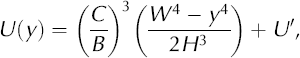
where U(y) is the downstream speed, H is ice thickness, Wis the ice-stream half-width, y is the distance from the center line toward the margin, C is the lateral shear stress, B is the flow hardness parameter and U’ is the speed at the margin. By matching only a section of the velocity profile, this technique quantifies the partitioning of the effective marginal shear stress and the basal shear stress ‘felt’ within each section. The shape of each polynomial is varied by adjusting ư and the ratio C/B. Figure 10 illustrates the segmented polynomial fits, and Table 2 summarizes the relevant parameter values along with the average root-mean-square misfit between the fits and the data. In both the 1985 and 1997 cases, the margin was taken to be a point of non-zero speed very close to the margin. In the margin sections at both epochs, the required fourth-order fit predicted a very high center-line velocity. Conversely, in both ‘shoulder’ sections, the margin velocity used was very high. In the center sections, most fits were flat across the fitted section, leaving little independent control on the two fitting parameters. Thus, the center sections were fit by matching the single velocity at the margin and the velocities across the center section.
Table 2. Comparison of derived parameters B, C, E and τ b (from Equations (1–3)) for the margin, shoulder and center sections of each transverse profile across the B2 portion of the ice plain of WIS using data from 1985 and 1997 (see also Fig. 10)

The ratio C/B is used to investigate the possible influences of basal shear stress and flow enhancement. By assuming a constant value of B, Ccan be calculated and subtracted from the driving stress, τ d, to estimate the basal shear stress, τb:
Values of τ d = 3.0±0.9kPa and B = 530 kPa aш are taken from Reference Joughin and TulaczykJoughin and others (2002) and the results shown in Table 2. The values of C reveal a consistent pattern for the two years. As expected, the largest values of C occur in the margin area. The lowest values occur in the shoulder area. The values in the center are still a major fraction of the driving stress, so the effect of lateral drag is strongly felt in the ice-stream center, in contrast to the interpretation of Reference Joughin and TulaczykJoughin and others (2002).
The basal stress pattern is clouded by large errors. A negative basal shear stress in the margins is untenable and is better explained by flow enhancement, which would lower the lateral shear stress. The corresponding flow enhancement can be calculated as
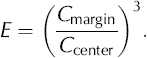
For 1985, E = 1.31, and for 1997, E = 1.29. These values are consistent with the detection of enhanced flow farther upstream (Reference Echelmeyer, Harrison, Larsen and MitchellEchelmeyer and others, 1994). In the shoulder area, the lower value of C suggests that here the basal stress is higher than elsewhere within the ice stream. Using other published values for τd and B (e.g. 2.58± 0.20 kPa and 428.6 kPa a1/3, respectively (Reference Bindschadler, Stephenson, MacAyeal and ShabtaieBindschadler and others, 1987)) changes the numbers somewhat, but not the general conclusions stated here.
Stress Changes
There are additional differences between the 1985 and 1997 profiles that express temporal changes in the stress regime along this transect. First, the kinematic center line shifted northward (Fig. 10). The uniformity of the velocities and the presence of a double maximum in the central portion of each profile make it difficult to quantify the change in halfwidth precisely. We used a conservative interpretation of a 2.8 km shift;however, the change in half-width could be interpreted to be as large as 21 km.
Lateral stresses appear to have increased from 1985 to 1997 in each of the three sections (Table 2). Although the changes are less than the errors, they are consistent. If there was not a corresponding increase in driving stress, this strongly suggests a decrease in basal stress, not an increase as Reference Joughin and TulaczykJoughin and others (2002) surmised from their till model. They calculated a 0.1 kPa (or 7%) increase in basal stress was required to decelerate WIS 1.4%a–1 for 14 years (i.e. 20%). Earlier in this paper, it was observed that in this region the large-scale surface slope of B1 increased 14% from 1984 to 1998 while the surface slope of B2 decreased 15% over the same period. Neither the thickness nor width of the ice stream changed as much, so it can be inferred that the driving stress exerted on B1 increased 14% while the driving stress on B2 decreased 15%. A driving-stress decrease coupled with a likely increase in lateral stress makes an increase in B2’s basal stress improbable.
Another change in the profiles is from nearly uniform velocities south of DNB in 1985 to a southward trend of decreasing velocity in 1997 (Fig. 10). The larger decelerations in the B1 flow of WIS, relative to the B2 flow, may be related to the 14% increase in large-scale surface slope of B1 as compared to the 15% decrease in B2’s surface slope. Deceleration of B1 in response to a possible increase in basal shear stress (inferred from an increased driving stress) fits better the situation mooted by Reference Joughin and TulaczykJoughin and others (2002). The differences between the temporal driving-stress patterns of B1 and B2 may invoke some additional cross-stream stress couplings that affect the lateral stress distribution and the observed shift in kinematic center line.
Flux
Elucidation of the changes in velocity and ice thickness enables us to comment on the variety of mass-balance calculations that have been undertaken in this area (Reference Thomas and BentleyThomas and Bentley, 1978; Reference Shabtaie, Bentley, Bindschadler and MacAyealShabtaie and others, 1988; Reference BindschadlerBindschadler and others, 1993). Occasionally, these calculations have produced contradictory results. The most comparable calculations are the series of gated boxes by Reference Shabtaie, Bentley, Bindschadler and MacAyealShabtaie and others (1988) and the Geographic Information System (GIS) approach of Reference BindschadlerBindschadler and others (1993).
The behaviors of the two major tributaries that form WIS (B1 and B2 in Fig. 5) are often discussed separately. Reference Shabtaie, Bentley, Bindschadler and MacAyealShabtaie and others (1988) calculated the mass balance of the ice plain by comparing fluxes across two gates (G5 and G6;see Fig. 5). These gates coincide with flight-lines along which ice-thickness data were available. Accumulation rates were taken from Reference Shabtaie and BentleyShabtaie and Bentley (1987). Velocities were mixed: SCP-era for G5 and RIGGS-era for G6. This was adjusted to a common velocity epoch by Reference BindschadlerBindschadler and others (1993), with the result that between gates G5 and G6 B2 was thickening while B1 was near equilibrium;however, both results were within one standard deviation of zero change (Fig. 12).

Fig. 12 Comparison of mass-balance calculations from three studies of the Whillans ice plain, for the area between gates G5 and G6 seen in Figure 5. None consider basal accumulation or melting, because it is unknown.
A similar result, but one that produced an estimate of the spatial pattern of thickness change, was computed by Reference BindschadlerBindschadler and others (1993) using a GIS approach. Integrating their results over the same area between gates G5 and G6 predicted thinning for both B1 and B2. Although of different sign than Shabtaie and others’ results, the 1σ range of possible rates, including no change, overlapped those of Reference Shabtaie, Bentley, Bindschadler and MacAyealShabtaie and others (1988) (Fig. 12). Accumulation rates for the two calculations are nearly identical. The claim by Reference Joughin and TulaczykJoughin and Tulaczyk (2002) that Reference Shabtaie and BentleyShabtaie and Bentley (1987) underestimate accumulation rates due to a conversion error has a negligible effect on our comparisons.
Our calculations here are made for boxes I–III, using the four flow-transverse flights and the two southernmost along- flow flights (Fig. 5). Calculations do not extend farther north because concurrent velocity data are not available. The 1998 SOAR ice thicknesses were sampled every 1 km after a 1 km averaging filter was applied. A bilinear interpolation was applied to determine surface speed from the 1997 SAR- derived surface velocities at the interpolated ice-thickness locations. Missing velocity data in three small gaps were filled by linear interpolation of the neighboring points. The surface velocity was assumed equal to the depth-averaged velocity because ice motion is dominated by sliding. A constant accumulation rate of 0.12 ma–1 (ice equivalent) was used;spatial variability of accumulation rate is not well determined, but minor variations would not affect the calculations significantly.
The mass balances are computed from the net volume flux into each box divided by the box area. The results are: box I, –0.08 ± 0.08 m a–1; box II, 0.02 ± 0.05 m a–1; and box III, 0.01 ± 0.07 m a–1 (ice equivalent). None are significantly different from zero, but the values suggest an overall pattern of slight thinning upstream and zero to slight thickening downstream. The combination of boxes I and II almost exactly coincides with the region between gates G5 and G6 of Reference Shabtaie, Bentley, Bindschadler and MacAyealShabtaie and others (1988). Our mass-balance result for the combination of boxes I and II is –0.02 ± 0.03 ma–1 and overlaps the previous estimates (Fig. 12). The smaller error for our result is achieved by using the more precise SOAR ice thicknesses and SAR-derived velocities.
Although zero change is included within the 1σ range of all the estimates discussed here, the mass balance for B2 is always above that for B1. Reference Joughin and TulaczykJoughin and Tulaczyk (2002) calculate a similar difference, with B2 in positive balance and B1 in negative balance for the entire ice stream. This has been attributed to the recent additional influx of ice into B2 that previously flowed farther north through Kamb Ice Stream (Reference Price, Bindschadler, Hulbe and JoughinPrice and others, 2001).
Reference Joughin and TulaczykJoughin and Tulaczyk (2002) discuss how the deceleration has shifted the mass balance of the ice stream from a negative state to one of near balance. This temporal imprint on B1’s mass balance across the ice plain is less obvious, possibly obscured by the larger errors of the earlier measurements (Fig. 12). A uniform deceleration will not create as large a shift in mass balance as would a spatial gradient in deceleration. The strongest indication of a spatial gradient in deceleration is from the larger decelerations closer to Crary Ice Rise. Elsewhere, the gradients are not significant, consistent with the zero mean change in ice- plain ice thickness.
Reference BindschadlerBindschadler (1997) has shown that the size and speed of ice streams cause flux perturbations to spread rapidly along the full length of the ice stream. The observation of only slight changes in mass balance confined to the ice-plain region and more significant changes over the whole ice stream is consistent with this view of rapid ice-stream adjustment to flux perturbations.
Summary
Perhaps no other region of West Antarctica better typifies the complexity of this ice sheet’s behavior than the Whillans ice plain. By virtue of its misidentification as part of the floating Ross Ice Shelf, the series of observations extend over more than four decades. Repeat observations of velocity and ice thickness lead to a large set of uniquely long datasets that we have presented together for the purpose of identifying past and ongoing changes as well as our examination of the most important factors responsible for those changes.
What has emerged is the clear picture that the deceleration of the ice plain is not caused by changes in the geometry of the area. Nor is it observed that the deceleration is creating significant widespread changes in the ice-plain geometry. Numerous local changes are observed and confirm that we would be able to see regional change if it existed. Grounding-line advance is detected in limited regions, and repeat satellite imagery is consistent with results from ground-based optical level lines. However, widespread changes in the extent of grounded ice are not observed.
Crary Ice Rise is seen to have the expected effect of thinning ice adjacent to its lateral margins, while ice immediately upstream is thickening and slowing faster than elsewhere across the ice plain. The ice rise’s influence extends only a few tens of kilometers upstream. Farther upstream, the central region of the ice plain shows a slight thinning, but the spatial variability is extremely high. The regions of largest change can be explained by local flow dynamics. Another isolated area of thickness change occurs just downstream of the ridge north of WIS, where local thickening upstream of a region of ice rumples is also associated with thinning downstream on the ice shelf.
This picture of thickness changes reflecting more local and less regional conditions is significant. It exposes the pitfall of over-interpreting local measurements as representative of regional conditions. This risk is often inherent in the mass-flux approach to mass-balance calculations and is likely a major contributor to the disparity between the series of mass-balance calculations made of this region and between these calculations and local measurements of ice-thickness change. One consistent characteristic that has emerged is that the northern half of the ice plain, fed by the northern branch of the ice stream, has a more positive mass balance than the southern half.
The dynamics of the Whillans ice plain is known to result from the balance of relatively small stresses. The measurement challenge inherent in this situation is amplified for the detection of changes in small stresses. Nevertheless, we find strong evidence of flow enhancement in the marginal ice, yet the flow of the central ice stream still feels the effect of the lateral resistance, contradicting the conclusions of Reference Joughin and TulaczykJoughin and others (2002).
The imprint of earlier deviations in the flow pattern of WIS is clear. Dating these past changes rests on weak assumptions about the past flow rates. The disagreements between flow-stripe orientations and current flow directions serve as a reminder that changes have probably been a persistent characteristic of WIS.
With minimal changes to the geometry of the ice plain, the deceleration of this ice is not in response to changes in driving stresses. Where the detailed pattern of deceleration is observed, the pattern is not consistent with the changes in driving stresses. Neither is it an effect of mass continuity since deceleration would require a widening (or thickening) of the ice stream to maintain the same flux at lower speed. If anything, there is a slight narrowing of the discharge path of WIS across the ice plain. We are led to conclude that the deceleration is driven by changing basal processes such as till properties, subglacial water supply or water pressure and that these changes are spatially variable. Direct measurement of such changes is difficult. Without verification of the cause, there is a need for continued monitoring of this region. Persistence would suggest that the deceleration of the ice and the increasing influence of Crary Ice Rise will continue;however, even the small changes in thickness and grounding will eventually manifest in significantly altered stresses and lead to additional changes in behavior of this ice stream and, possibly, its neighboring ice streams.
Acknowledgements
We thank I. Joughin for the 1997 SAR-derived velocities, D. Blankenship and SOAR for their laser altimeter-derived surface elevations and radar-derived ice thicknesses, and M. Lythe for providing many of the RIGGS data used in this analysis. H. Conway and a second anonymous reviewer provided constructive comments that guided us to an improved revision of the manuscript. The work was supported by NSF grant OPP-9616394.


