


1. INTRODUCTION
Alaska is home to seven major glacierized mountain ranges, with topography spanning from sea level to 6190 m a.s.l. at the summit of Denali, North America's highest mountain. Combined with a high-latitude setting and abundant precipitation, this topography gives rise to glaciers covering similarly large altitudinal ranges. Twenty-four Alaska glaciers have elevation ranges in excess of 4000 m, with a combined area of over 17 000 km2, or 20% of the total glacierized area in Alaska (Kienholz and others, Reference Kienholz2015). Of these, eight glaciers totaling 11 800 km2 in area, or 14%, have elevation ranges > 5000 m, including the Kahiltna Glacier with a span of 5844 m.
Altogether, the glaciers of Alaska and Northwestern Canada (hereafter called Alaska glaciers for brevity) are shedding mass due to climate change at one of the highest rates of any mountain glacier system (Arendt and others, Reference Arendt, Echelmeyer, Harrison, Lingle and Valentine2002; Meier and others, Reference Meier2007; Berthier and others, Reference Berthier, Schiefer, Clarke, Menounos and Rémy2010; Wu and others, Reference Wu2010; Jacob and others, Reference Jacob, Wahr, Pfeffer and Swenson2012; Sasgen and others, Reference Sasgen, Klemann and Martinec2012; Arendt and others, Reference Arendt2013; Gardner and others, Reference Gardner2013; Larsen and others, Reference Larsen2015), with global and regional consequences. At the global scale, between 2003 and 2009, Alaska glaciers contributed an estimated 20% of the mean sea-level rise from mountain glacier mass loss, including the Greenland and Antarctic peripheries but excluding the ice sheets themselves (Arendt and others, Reference Arendt2013; Gardner and others, Reference Gardner2013). At the regional scale, Alaska glacier runoff constitutes an estimated 38% (Neal and others, Reference Neal, Hood and Smikrud2010) to 47% (Beamer and others, Reference Beamer, Hill, Arendt and Liston2016) of the total annual land-to-ocean freshwater flux into the Gulf of Alaska, acting as a principal driver of the Alaska Coastal Current that delivers crucial nutrients and freshwater to coastal ecosystems (Royer, Reference Royer1981). In their recent study, Larsen and others (Reference Larsen2015) used repeat laser altimetry data to derive a mass change of −75 ± 11 Gt a−1 for all Alaska glaciers between 1994 and 2013, an estimate that best represents our current state of knowledge. Uncertainty in their estimate was largely due to extrapolation from surveyed to unsurveyed glaciers, given substantial glacier-to-glacier variability in mass loss due to the wide range of glacier types (tidewater, lake-, and land-terminating), sizes, and geometries.
In this study, we propose that glaciers with large altitudinal ranges represent a unique class of glacier geometry requiring special consideration in mass-balance studies. As these glaciers are subject to different climatic regimes along their elevation ranges, extrapolation of ground-based measurements (where they exist) is very challenging, and mass-balance modeling with those datasets is difficult. These limitations are not unique to Alaska, but are equally problematic in other remote and topographically extreme areas such as High Mountain Asia, the Antarctic Peninsula and the Canadian High Arctic. For regions like these, it is only in combining multiple methods and datasets that we can better understand how these glaciers may respond differently to climate change, therefore reducing uncertainty in long-term mass balance, as well as providing information on subannual and annual changes. Capturing all of these elements is crucial for quantifying seasonal runoff, characterizing physical processes important for modeling future conditions, and partitioning runoff into rain, snow and ice melt, information that is vital for downstream ecosystem studies.
Here, we use mixed methods to reconstruct the 1991–2014 mass balance of the Kahiltna Glacier in the Central Alaska Range. The Kahiltna spans one of the greatest elevation ranges of any glacier in Alaska and globally (264-6108 m a.s.l. near the summit of Denali), and is therefore not a type of glacier conventionally chosen for mass-balance studies. We use an enhanced temperature index model to link methods and generate a time series of mass changes, calibrated to glacier-wide balance estimates from repeat laser altimetry and point balance observations, and validated against gravimetry data from NASA's Gravity Recovery and Climate Experiment (GRACE) satellites. We also compare our results with a historic National Park Service (NPS) single-stake index site observational record, finding poor correlation between those measurements and our modeled glacier-wide balances (R 2 = 0.22 and p = 0.03), suggesting that the single-stake method's ability to predict glacier-wide balances is limited. By examining several methods, we are able to assess both subannual and long-term (decade scale) changes for the Kahiltna Glacier that are otherwise not captured by any single method. In addition to providing a better estimate for the Kahiltna Glacier, we make recommendations for improving monitoring efforts for other remote glaciers of extreme altitudinal range, toward improving mass change estimates in other high-relief mountain ranges globally.
2. STUDY AREA
The Kahiltna Glacier, centered at 62.78°N and 151.30°W, is the largest glacier in the Alaska Range, with an area of 503 km2 and centerline length of 78 km including its debris-covered terminus (Fig. 1). Elevations span between 264 m a.s.l. at the terminus to 6108 m a.s.l. near the summit of Denali (statistics from Kienholz and others, Reference Kienholz2015), one of the greatest elevation ranges of any glacier globally.

Fig. 1. (a) Location of the Central Alaska Range within Alaska. (b) Location of the Kahiltna Glacier, outlined in blue, within the glaciers of the Central Alaska Range, outlined in gray. The NOAA weather station at Talkeetna and the nearest NCEP-NCAR reanalysis product node are also shown, along with the UAF laser altimetry flight path and GRACE solution mascon grid cell encompassing the Kahiltna Glacier (purple box). (c) Locations of ground observation datasets used for model input or calibration, including our AWS, air temperature sensors, mass-balance sites, and snow depth measurements.
The Alaska Range acts as an orographic barrier to dominant moist weather systems entering inland off the Gulf of Alaska. It is therefore at the climatic divide between the coastal Cook Inlet climatological zone and the more continental Central Interior, as defined in Bieniek and others (Reference Bieniek2012). Larsen and others (Reference Larsen2015) point out that glaciers often reside at the divide between climatological zones and that glacierized regions therefore do not always correspond to general patterns of temperature and precipitation observed within the rest of the zone. Particularly in terms of precipitation, the Kahiltna Glacier resides in this difficult-to-characterize zone, as it is a large distance from the coast (168 km), but on the windward side of the range between three of the ten highest peaks in North America. In other words, while the glacier's continentality connotes low amounts of snowfall, its local topography connotes higher amounts.
Together with the glacier's large size and elevation range, these features present a challenge for collecting field data, for extrapolating from data collected at other sites in Alaska, or for characterizing on-glacier climatological conditions using available data products.
3. DATA
To reconstruct the 1991–2014 surface mass balance of the Kahiltna Glacier, we used an enhanced temperature index model calibrated using a volume change estimate from laser altimetry elevation data from 1994 and 2013, and mass-balance measurements from field campaigns in 2010 and 2011. We then independently compare our model results with mass-balance measurements from the National Park Service (NPS), and to mass-balance estimates derived from NASA's GRACE satellites, neither of which are used in model calibration. The model requires as input: a DEM; glacier outline and surface-type information; and climate data including daily temperature and lapse rates, and precipitation data at one location.
3.1. Laser altimetry elevation data
Repeat laser altimetry measures elevation changes over time from which volume change is estimated and mass change inferred. We obtain glacier-wide mass-balance estimates determined from airborne centerline laser altimetry data collected by the NASA Operation IceBridge group at the University of Alaska Fairbanks, using methods described in Johnson and others (Reference Johnson, Larsen, Murphy, Arendt and Zirnheld2013) and Larsen and others (Reference Larsen2015) (further details are outlined in the ‘Methods’ section). The flight profile for the Kahiltna Glacier is shown in Figure 1. We use estimates derived from surveys carried out on 31 July 1994 and 28 May 2013, providing the longest overlap with our modeling period.
3.2. Mass-balance measurements – 2010/11
We carried out point mass-balance observations on 30 April– 4 May and 22 Sept 2010, and 24–30 April and 14 Sept 2011, following the standard methods (Østrem and Brugman, Reference Østrem and Brugman1991; Mayo, Reference Mayo2001; Cogley and others, Reference Cogley2011). Measurements fell along the glacier centerline spanning elevations from 800 to 1400 m a.s.l., a range that was limited by safe travel conditions, and that represents ~ 25% of the glacier area (Fig. 1). Two additional sites were also monitored at 1800 and 2100 m a.s.l. in 2011, but these represent shorter-term measurements between 6 June and 15 Aug 2011. Altogether, ablation stakes were installed at nine elevations in 2010 and 11 elevations in 2011. Water equivalent values for ice melt were calculated using an assumed ice density of 900 kg m−3. Winter balances were derived each year at these same locations as well as approximately 75 additional locations between 800 and 1400 m a.s.l. along two lateral transects and the glacier centerline, using measured snow depths and an average annual depth-density profile determined from two to three snow pits.
3.3. Mass-balance measurements – NPS – 1991-2014
Mass-balance monitoring on the Kahiltna Glacier was pioneered in 1991 by the NPS in conjunction with the United States Geological Survey (USGS) (Mayo, Reference Mayo2001) according to the single-stake method. The effort continues today as part of the NPS vital signs monitoring plan (MacCluskie and others, Reference MacCluskie, Oakley, McDonald and Wilder2005), and represents the third-longest continuous program of mass-balance measurements on any Alaska glaciers.
Spring and fall mass balances are measured annually using conventional glaciological methods, on a floating date system. Measurements are carried out at a single location near each glacier's equilibrium line altitude (ELA), as determined from balance gradients derived between 1992 and 1995 from two stakes installed at 1540 and 1930 m a.s.l. (Burrows and Adema, Reference Burrows and Adema2011). Using the derived balance gradient and the elevation of each annual measurement, the NPS calculates the long-term average ELA for the Kahiltna Glacier of 1925 m a.s.l., yielding an accumulation-area-ratio of ~0.47.
3.4. GRACE
To independently validate the modeled mass change time series, we turn to GRACE gravimetry data. The tandem GRACE satellites, launched in 2002, use a microwave K-band intersatellite ranging system to measure changes in Earth's gravity field. Forward-modeling is used to account for time-varying gravity signals from Earth and ocean tides, atmosphere, and terrestrial water storage, and the residual signal is assumed to represent glacier mass balance (Wouters and others, Reference Wouters2014).
The primary benefit of using GRACE data is the high temporal resolution of mass variations that provides information at subannual and annual timescales. However, estimates of mass balance from GRACE are prone to contamination from nonglacial sources, and to signal leakage between adjacent grid cells in the spatial domain. Moreover, as the fundamental GRACE resolution is a 300 km Gaussian spatial smoothing filter (Luthcke and others, Reference Luthcke2013), estimates of mass balance from processed GRACE solutions are limited to very coarse spatial resolutions. We note that the novel comparison of a GRACE solution with modeling results for an individual glacier is made possible primarily given the Kahiltna Glacier's large size (503 km2) within the total glacierized area (3236 km2) contained in the GRACE mascon (~12 390 km2). Although in this case simple spatial downscaling methods are possible to gain subannual information for a smaller area such as an individual glacier, as we demonstrate in this study, it is not expected that the magnitude of the long-term mass change trend will necessarily be accurate.
At the regional scale, GRACE has been applied extensively to estimate mass loss from Alaska glaciers in recent years (Tamisiea and others, Reference Tamisiea, Leuliette, Davis and Mitrovica2005; Chen and others, Reference Chen, Wilson and Tapley2006; Luthcke and others, Reference Luthcke, Arendt, Rowlands, Larsen and McCarthy2008; Pritchard and others, Reference Pritchard, Luthcke and Fleming2010; Wu and others, Reference Wu2010; Jacob and others, Reference Jacob, Wahr, Pfeffer and Swenson2012; Sasgen and others, Reference Sasgen, Klemann and Martinec2012; Arendt and others, Reference Arendt2013; Luthcke and others, Reference Luthcke2013). The range of publications reflects variations in Level 1 GRACE products from different processing centers, as well as differences in methods for filtering and correcting the observations to isolate glacier mass balances from other sources of mass change. We use GRACE data acquired from NASA Goddard Space Flight Center Geodesy Laboratory's high-resolution mass concentration (mascon) solution (Luthcke and others, Reference Luthcke2013). This solution provides mass change estimates at ~30-day intervals and 1° × 1°(~12 390 km2) resolution.
We choose this dataset because it is one of few that explicitly corrects for local mass increases associated with post-Little Ice Age disintegration of the Glacier Bay icefield (Larsen and others, Reference Larsen, Motyka, Freymuller, Echelmeyer and Ivins2005). It also compares well with regional-scale Gulf of Alaska mass-balance model simulations (Hill and others, Reference Hill, Bruhis, Calos, Arendt and Beamer2015) and to mass loss estimates from NASA's Ice, Cloud and Land Elevation Satellite (ICESat) (Arendt and others, Reference Arendt2013). However, although the dataset includes spatial and temporal constraints over the entire glacierized Alaska region, no constraints are applied at the resolution of individual mascons. This limits uncertainty assessment at these spatial scales. However, several studies have found good agreement between laser altimetry and GRACE mascons summed over the Glacier Bay and St. Elias regions (Arendt and others, Reference Arendt2008; Johnson and others, Reference Johnson, Larsen, Murphy, Arendt and Zirnheld2013), supporting our choice of this dataset for helping characterize changes at a sub-regional scale. We focus on the mascon encompassing the majority of the Central Alaska Range, which includes 98% of the Kahiltna Glacier (Fig. 1).
3.5. DEM
For input for the 1991–2014 model simulations, we use an Interferometric Synthetic Aperture Radar (IFSAR) DEM. The IFSAR DEM is based on X-band (3 cm wavelength) imagery acquired in July 2010 for the Alaska Statewide Digital Mapping Initiative, now available as part of the USGS National Elevation Dataset (Gesch and others, 2002; Gesch, Reference Gesch2007). The IFSAR DEM has horizontal and vertical datum of NAD83 and NAVD88. We resample the 5 m postings to 50 m for model simulations.
3.6. Glacier outline and surface-type information
We use an outline for the Kahiltna Glacier from the Randolph Glacier Inventory v3.2 (Pfeffer and others, Reference Pfeffer2014; Kienholz and others, Reference Kienholz2015). These outlines are derived from a mosaic of Landsat 5/7 ETM+ images from the mid-2000s using a semiautomated approach with manual adjustments to ensure that debris-covered ice is included. Our outline contains the main Kahiltna Glacier polygon, and several small polygons of high-altitude hanging ice that avalanche into the Kahiltna Glacier basin. A comparison of this outline to one derived from historical USGS topographical maps shows only minor glacier area change (5.4% reduction) in over 50 years (Loso and others, Reference Loso, Arendt, Larsen, Rich and Murphy2014). For our model simulations, we therefore assume that modifying the glacier extent over time can be neglected.
In the model, we also differentiate between surface types at each grid cell. Firn areas are located at elevations above the long-term ELA established by the NPS (1925 m a.s.l.). The Kahiltna Glacier's terminal debris cover map comes from the Alaska-wide glacier inventory compiled by Kienholz and others (Reference Kienholz2015), who derived the map using a band ratioing technique applied to Landsat 5 imagery, following a similar method as in Paul and others (Reference Paul, Huggel and Kääb2004).
3.7. Climate data
Our model simulations depend on air temperature and precipitation data from two sources: (1) on-glacier sensors deployed in 2010 and 2011; (2) a 1991–2014 reanalysis product. We also indirectly use gradients from a gridded precipitation product to help guide our decisions on precipitation distribution.
3.7.1 Air temperature and lapse rates
Onset HOBO U23 Pro v2 sensors installed on floating stands recorded 2 m air temperature at five elevations on the glacier between ~800 and 1400 m a.s.l., from 6 May to 22 Sept 2010 and 30 April to 13 Sept 2011. To extend our dataset in time from 1 Oct 1991 to 12 June 2014, we compare our on-glacier measurements to temperature datasets from: (a) a National Oceanic and Atmospheric Administration (NOAA) airport weather station in Talkeetna, 60 km southeast of the glacier at 62.32°N and 150.09°W; and (b) an upper-air reanalysis climate data product from the National Centers for Environmental Prediction and National Center for Atmospheric Research (hereafter simply NCEP–NCAR) (Kalnay and others, Reference Kalnay1996), at a node located ~60 km west of the glacier at 62.50°N and 150.50°W. We use the daily product ‘NOAA NCEP–NCAR CDAS-1 mc8110,’ based on a 1981 to 2010 climatology and available at a spatial resolution of ~2.5° × 2.5° (Kalnay and others, Reference Kalnay1996). Temperature data from NCEP–NCAR correlates best with our on-glacier measurements for the overlapping time period. In particular, temperatures from the 850-hPa isobar level (corresponding to a mean atmospheric height of 1370 m a.s.l.) correlate better (R 2 = 0.75) than other levels or from interpolation between isobar geopotential heights to our on-glacier temperature sensor elevations (all R 2 = 0.70). The strong correlation with the 850-hPa isobar in particular agrees with previous findings (Rasmussen and Conway, Reference Rasmussen and Conway2004). Note that in all cases (i.e. for all NCEP–NCAR isobars examined, and for interpolation between isobars), we compare the NCEP–NCAR record to each of our five temperature sensors, and find the best correlation at our highest-elevation sensor (1400 m a.s.l.). As input for model simulations, we therefore downscale the 850-hPa NCEP–NCAR record to this sensor elevation by bias correction using a bilinear transfer function (Fig. 2) to determine temperatures T in °C:
 $$ T = \left\{\matrix{ 0.31 \lpar T_{{\rm NCEP}}\rpar + 0.58\comma & T_{{\rm NCEP}} \geq T_{{\rm o}}\cr 0.98 \lpar T_{{\rm NCEP}}\rpar - 0.39\comma & T_{{\rm NCEP}} < T_{{\rm o}} } \right. $$
Fig. 2. Daily mean air temperature from NCEP–NCAR upper-air climate product at the 850-hPa isobar level, versus temperature measured at 2 m above the ground (sensor height) at 1400 m a.s.l. on the Kahiltna Glacier. A bilinear transfer function was used to fit the data (solid black lines) for temperatures above (grey) and below (black) T NCEP = 0.5°C.
After manually exploring multiple values, the intersection point T o = 0.50°C is found to minimize RMSE for both regressions (1.22°C for T NCEP < T o, 0.59°C for T NCEP ≥ T o).
Average monthly summer lapse rates are calculated for model input from linear regression between all five sensors for both years. Lapse rates show some seasonality, with a generally smaller temperature decrease with elevation in mid-summer, ranging from −0.47°C(100 m)−1 in May to −0.28/ − 0.33°C(100 m)−1 in June/July. The calculated values were tested for sensitivity to the removal of any one sensor from the dataset by leave-one-out cross-validation, with negligible effect. Lapse rates for winter months outside of our measurement window (October–March) are assumed to have the same value as the month of April (−0.43°C(100 m)−1), as this is the only monitored month with full snow cover over that elevation range.
3.7.2 Precipitation
Timing of snowfall events for the 1 Oct 1991 to 12 June 2014 model period is from NCEP–NCAR reanalysis data. The product shows good agreement with the timing of events recorded at a MaxBotix MB7060 sonic ranger we installed at 1200 m a.s.l. on the glacier during the winter of 2010/11, but precipitation event magnitudes were corrupted by instrumental error. This agreement increases our confidence that the reanalysis product is simulating the timing of events correctly.
To then scale precipitation magnitudes from the NCEP–NCAR node to our weather station location on the Kahiltna Glacier, we compare cumulative snowfall from NCEP–NCAR to our in situ mass-balance measurements at the corresponding observation dates. We are cautious against taking any single-point measurement as fully representative of winter balance at that elevation, given the large variability between measurements (Fig. 3). This is likely due to differential snow deposition over the considerable ice surface topography in the ablation area (i.e. local surface troughs and valleys of the order of 1–2 m high), a characteristic often seen on large valley glaciers. As a result, we elect to use a precipitation correction factor p corr (a multiplicative factor applied to NCEP–NCAR data) as a tuning parameter in the model, rather than assign a single-scaling value. As our combined 2010 and 2011 winter balance measurements are non-normally distributed, we use the interquartile range, from which we derive scaling values for p corr from 377 to 488%. These high values point to a noteworthy underestimation of precipitation attributed to this region by NCEP–NCAR compared with our in situ observations. On the linear regression curve for our observations with elevation, the elevation corresponding to the median value for p corr, 432%, is the same as the automated weather station (AWS) elevation used to bias-correct our NCEP–NCAR temperature record (Fig. 3). All climate variables serving as input into the model are therefore corrected to that single AWS elevation.
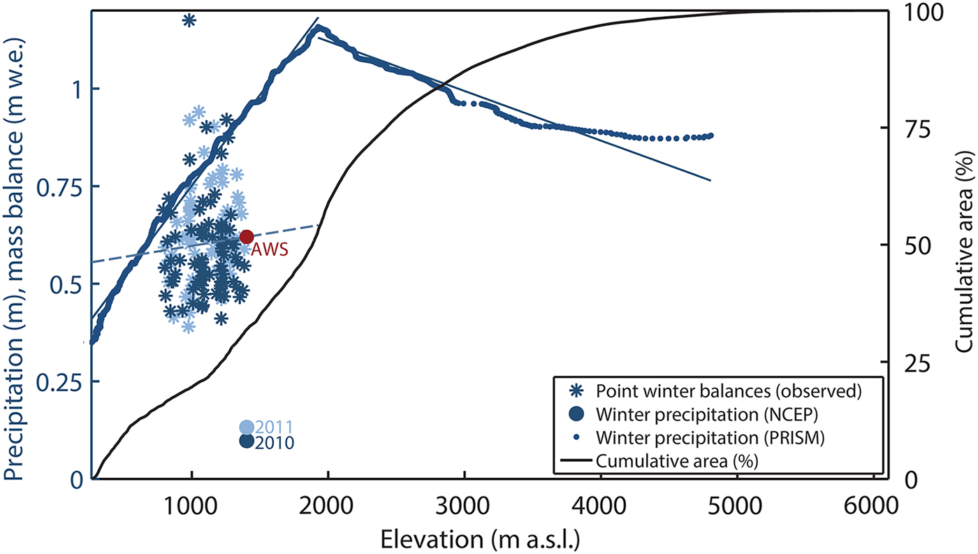
Fig. 3. Left axis: winter precipitation and winter mass-balance datasets used for scaling and spatially distributing NCEP–NCAR precipitation records for model input. Dark blue (2010) and light blue (2011) stars show point winter balance measurements, with linear trend with elevation for both years shown as a dashed blue line. Large blue dots represent cumulative precipitation from NCEP–NCAR at the same elevation as our on-glacier AWS, used for scaling precipitation magnitudes to our observations. Winter balance at our AWS is shown in red, which is equivalent to the median winter balance value for all observations, and which falls along the linear trend for all observations. Small dots represent Oct–April precipitation sums from the PRISM climatology product for the Kahiltna Glacier, binned by elevation, for use in spatially distributing scaled precipitation events from NCEP–NCAR. Linear trends for PRISM are shown for elevations below and above 1925 m a.s.l. (Note that PRISM grid cells are too large to accurately resolve elevations in excess of ~4800 m a.s.l.). Right axis: the glacier's hypsometry, expressed as the cumulative glacier area below a given elevation in %, is shown.
To spatially distribute precipitation events from the weather station location to the full glacier extent, we opt not to rely exclusively on the linear elevation dependence from our measurements, because the trend is not robust amid high variability over the elevations sampled (R 2 = 0.0056 and p = 0.34; Fig. 3). We look instead to 2 × 2 km grids of monthly average precipitation from 1971 to 2000 from the Parameter-elevation Regression on Independent Slopes Model (PRISM) climate product (Daly and others, Reference Daly, Neilson and Philips1994, Reference Daly, Gibson, Taylor, Johnson and Pasteris2002), which assign one precipitation regime to elevations <1925 m a.s.l., and above which a rainshadow effect seems to weaken precipitation (Fig. 3). However, we find that the PRISM gradient for elevations <1925 m a.s.l. is too steep, as preliminary model simulations yield winter balances at low elevations (<500 m a.s.l.) that are negative, a result that is incongruent with our late-winter visual examination by fly-over. For elevations <1925 m a.s.l., we therefore choose to vary the precipitation gradient as a tuning parameter p grad, ranging between the lower limit value obtained from linear regression of our combined 2010 and 2011 observations (n = 167, 5.71 mm w.e. (100 m)−1 elevation) and the upper limit value obtained from PRISM (47.30 mm w.e. (100 m)−1). For lack of any information at high elevations, we elect to apply the PRISM gradient for the ~47% of the glacier area with elevations ≥1925 m a.s.l. (−11.30 mm w.e. (100 m)−1).
4. METHODS
4.1. Model application
Mass-balance modeling uses climate data (e.g. air temperature, melt, and snowfall) to generate a time series of glacier mass balances at every grid cell within a domain (Hock, Reference Hock2003, Reference Hock2005). We implement the open-access Distributed Enhanced Temperature-Index Model (DETIM; http://regine.github.io/meltmodel/) (Hock, Reference Hock1999). The model is driven by daily near-surface air temperature, precipitation, and temperature lapse rate input. Air temperature is used as a proxy for the dominant energetic processes of ablation, including radiation and turbulent heat fluxes. Shading is taken into account using solar geometry and surrounding topography, by implementing an algorithm that determines the mean potential solar radiation for each grid cell, a physically based addition that generally improves mass-balance model performance (Mosier and others, Reference Mosier, Hill and Sharp2016). Daily melt is determined for either a snow- or ice-covered grid cell by:
 $$ M = \left\{\matrix{ \lpar F_{{\rm m}} + a_{{\rm snow\comma\ ice}}* \! I \rpar * \; F_{{\rm deb}}* \; T\comma \; T \gt 0\cr 0\comma \hfill T \leq 0 } \right. $$
where M is melt in m w.e., F m is the melt factor in mm d−1 °C−1, a snow and a ice are the radiation factors for snow and ice in mm m2W−1d−1 °C−1, I is the potential direct solar radiation calculated at every time step (daily), F deb is a multiplicative factor for melt suppression under debris, and T is the air temperature in °C. Note that a snow must be smaller than or equal to a ice, given generally higher albedo over snow than bare ice, and that F deb = 1 for all grid cells that are not debris-covered. Our suite of six tuning parameters is made up of these four empirical parameters F m, a snow, a ice, and F deb, along with the precipitation correction factor p corr that scales precipitation amounts from the NCEP–NCAR record in percent, and the precipitation gradient p grad that spatially extrapolates precipitation to elevations <1925 m a.s.l. in mm w.e. (100 m)−1.
We choose to alter the factor for melt suppression under debris as one of our model tuning parameters, F deb, as we are limited to only five ground observations of debris thickness on the Kahiltna Glacier, averaging 3 cm. We therefore use a multiplicative factor varying from 1.00 to 0.70, corresponding to a range of debris thickness from 0 to 3 cm as per Evatt and others (Reference Evatt2015), a study that derived a physical relationship between debris layer thickness and melt suppression, in agreement with numerically derived relationships and empirical observations from a previous work (Nicholson and Benn, Reference Nicholson and Benn2006).
We assign a fixed precipitation threshold temperature range of 0.50–2.50°C (Rohrer, Reference Rohrer1989), meaning that all precipitation falls as snow for any temperature below 0.50°C, as rain above 2.50°C, and with a linear interpolation of the percentage of snow and rain that falls within that range. Rain is not considered as a contributor to mass balance.
4.2. Laser altimetry
We obtain the estimate for the glacier-wide annual mass-balance rate for 31 July 1994 to 28 May 2013 from the University of Alaska Fairbanks Operation IceBridge team, who generate these estimates according to the published methods in Johnson and others (Reference Johnson, Larsen, Murphy, Arendt and Zirnheld2013) and Larsen and others (Reference Larsen2015). Their approach derives height change rate (dh/dt) profiles from the repeat centerline data, integrates these over the full glacier hypsometry obtained from the Randolph Glacier Inventory (Pfeffer and others, Reference Pfeffer2014; Kienholz and others, Reference Kienholz2015), and calculates a mass change estimate by means of a density assumption. Lateral extrapolation assumes no errors in the glacier hypsometries, and that the centerline elevation changes are representative of the full glacier width. Larsen and others (Reference Larsen2015) employ a density of 850 ± 60 kg m−3 to arrive at a water equivalent value, based on findings in Huss (Reference Huss2013). This value, which is lower than the conventional 900 kg m−3 often used to convert geodetic changes to volume loss based on Sorge's Law (Bader, Reference Bader1954), is explained by the removal of low-density firn layers with negative balance – a choice we believe is appropriate for the Kahiltna Glacier, given its large firn area (Gusmeroli and others, Reference Gusmeroli2013) that continues to be exposed by recent mass losses.
Error for the airborne laser altimetry balance estimates for individual glaciers are also detailed in Johnson and others (Reference Johnson, Larsen, Murphy, Arendt and Zirnheld2013) and Larsen and others (Reference Larsen2015). The dominant sources of measurement error of the altimetry method are associated with sensor and aircraft positioning errors, crevasse advection and lateral extrapolation. Together, these errors contribute to an elevation change rate uncertainty for each elevation bin that is integrated over the glacier hypsometry, then multiplied in quadrature with density uncertainties to arrive at a mass-balance uncertainty.
4.3. GRACE
The Luthcke and others (Reference Luthcke2013) solution for the mascon surrounding the Central Alaska Range (Fig. 1) provides a time series of cumulative mass change in m w.e. for the entire domain, beginning from an arbitrary zero point. We scale this time series by the ratio of the area of all glacier ice to the full mascon area, to get mass changes for the ice-covered portions of the domain only. Therefore, the cumulative balance results below actually represent changes for all glacier ice within the mascon rather than only the Kahiltna Glacier.
For comparison with our model results we extract each year's maximum and minimum from the modeled cumulative balance curve from which we compute summer, winter and annual balances in the stratigraphic time system (Cogley and others, Reference Cogley2011), as was done in Luthcke and others (Reference Luthcke, Arendt, Rowlands, Larsen and McCarthy2008, Reference Luthcke2013). This simple approach is acceptable given that mass turnover in the Gulf of Alaska region has a very clean seasonal signal with little noise (Luthcke and others, Reference Luthcke2013).
4.4. Model calibration & validation
We calibrate the model by adjusting six parameters: melt factor F
m; radiation factors for snow a
snow and ice a
ice; precipitation gradient p
grad for elevations <1925 m a.s.l.; precipitation correction factor p
corr; and factor for melt suppression under debris F
deb. We perform 1800+ model simulations by beginning with a broad grid search across the parameter space, then focusing in on several local subspaces with a finer grid. We consider two calibration criteria. First, we seek to match an estimate for glacier-wide mass balance derived from laser altimetry for the period spanning from 31 July 1994 and 28 May 2013. We find those simulations with a mass-balance rate $\dot {B}$
for this exact period that is within +/ − 10% of the target laser altimetry-derived mean annual balance rate
$\dot {B}$
for this exact period that is within +/ − 10% of the target laser altimetry-derived mean annual balance rate $\dot {B}$
of −0.73 m w.e. a−1. Second, from that subset, we find simulations whose model-generated point balances best approximate measurements in an RMSE sense, choosing those simulations with RMSE ranging from 0.53 to 0.58 m w.e., i.e. within 5% of the smallest RMSE in that subset (~0.53 m w.e.). This yields a set of 17 simulations. Figure 4 is a visual representation of our full searched 6-D parameter space showing the parameter combinations closest to the target value, −0.73 m w.e. a−1. Figure 5 shows the fit of modeled to measured point balances for the subset of 17 simulations, and Figure 6 shows a scatter plot of modeled to measured point balances for the single best-performing simulation. This calibration approach prioritizes matching the long-term geodetic balance over the point balance measurements, particularly given that the latter quantity exhibits substantial variability due to ice surface topography that is not well-captured by the model. This means sacrificing goodness-of-fit to our measured point balances, as it increases the RMSE value from the 1800+ simulation minimum of 0.44 m w.e. Our best-performing model simulations also consistently overestimate the steepness of the measured summer and winter balance gradients over the small elevation range sampled (~800–1400 m a.s.l.), as was similarly found in another recent temperature index modeling study on Alaska's Yakutat Glacier (Trüssel and others, Reference Trüssel2015). We accept this as a cost of emphasizing the long-term mass change as our first priority.
$\dot {B}$
of −0.73 m w.e. a−1. Second, from that subset, we find simulations whose model-generated point balances best approximate measurements in an RMSE sense, choosing those simulations with RMSE ranging from 0.53 to 0.58 m w.e., i.e. within 5% of the smallest RMSE in that subset (~0.53 m w.e.). This yields a set of 17 simulations. Figure 4 is a visual representation of our full searched 6-D parameter space showing the parameter combinations closest to the target value, −0.73 m w.e. a−1. Figure 5 shows the fit of modeled to measured point balances for the subset of 17 simulations, and Figure 6 shows a scatter plot of modeled to measured point balances for the single best-performing simulation. This calibration approach prioritizes matching the long-term geodetic balance over the point balance measurements, particularly given that the latter quantity exhibits substantial variability due to ice surface topography that is not well-captured by the model. This means sacrificing goodness-of-fit to our measured point balances, as it increases the RMSE value from the 1800+ simulation minimum of 0.44 m w.e. Our best-performing model simulations also consistently overestimate the steepness of the measured summer and winter balance gradients over the small elevation range sampled (~800–1400 m a.s.l.), as was similarly found in another recent temperature index modeling study on Alaska's Yakutat Glacier (Trüssel and others, Reference Trüssel2015). We accept this as a cost of emphasizing the long-term mass change as our first priority.

Fig. 4. Parameter combinations for the 17 best-performing model simulations (i.e. with results closest to the target $\dot {B}$
value of −0.73 m w.e. a−1 for 1994–2013). F
m is the melt factor in mm d−1 °C−1, a
ice and a
snow are the radiation factors for snow and ice in mm m2W−1d−1 °C−1, F
deb is melt suppression under debris as a multiplicative factor, the precipitation gradient p
grad for elevations <1925 m a.s.l. is in mm w.e. (100 m)−1 elevation, and the precipitation correction factor p
corr is in percent. Values on the left and right axes show the end members of the full parameter space searched in our 1800+ simulations. Annotations within the graph indicate the number of successful occurrences of a particular parameter value.
$\dot {B}$
value of −0.73 m w.e. a−1 for 1994–2013). F
m is the melt factor in mm d−1 °C−1, a
ice and a
snow are the radiation factors for snow and ice in mm m2W−1d−1 °C−1, F
deb is melt suppression under debris as a multiplicative factor, the precipitation gradient p
grad for elevations <1925 m a.s.l. is in mm w.e. (100 m)−1 elevation, and the precipitation correction factor p
corr is in percent. Values on the left and right axes show the end members of the full parameter space searched in our 1800+ simulations. Annotations within the graph indicate the number of successful occurrences of a particular parameter value.
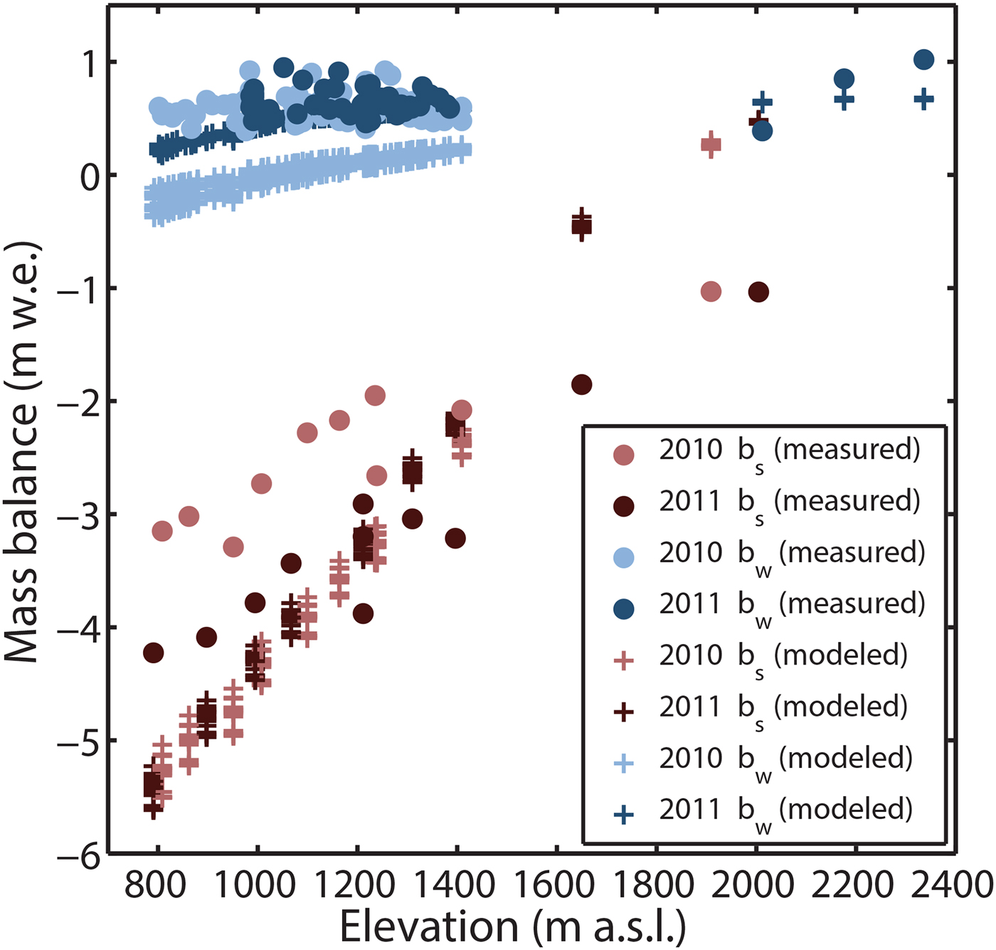
Fig. 5. Modeled (representing the 17 best-performing simulations) and measured point mass balances as a function of elevation over the range of altitudes sampled.
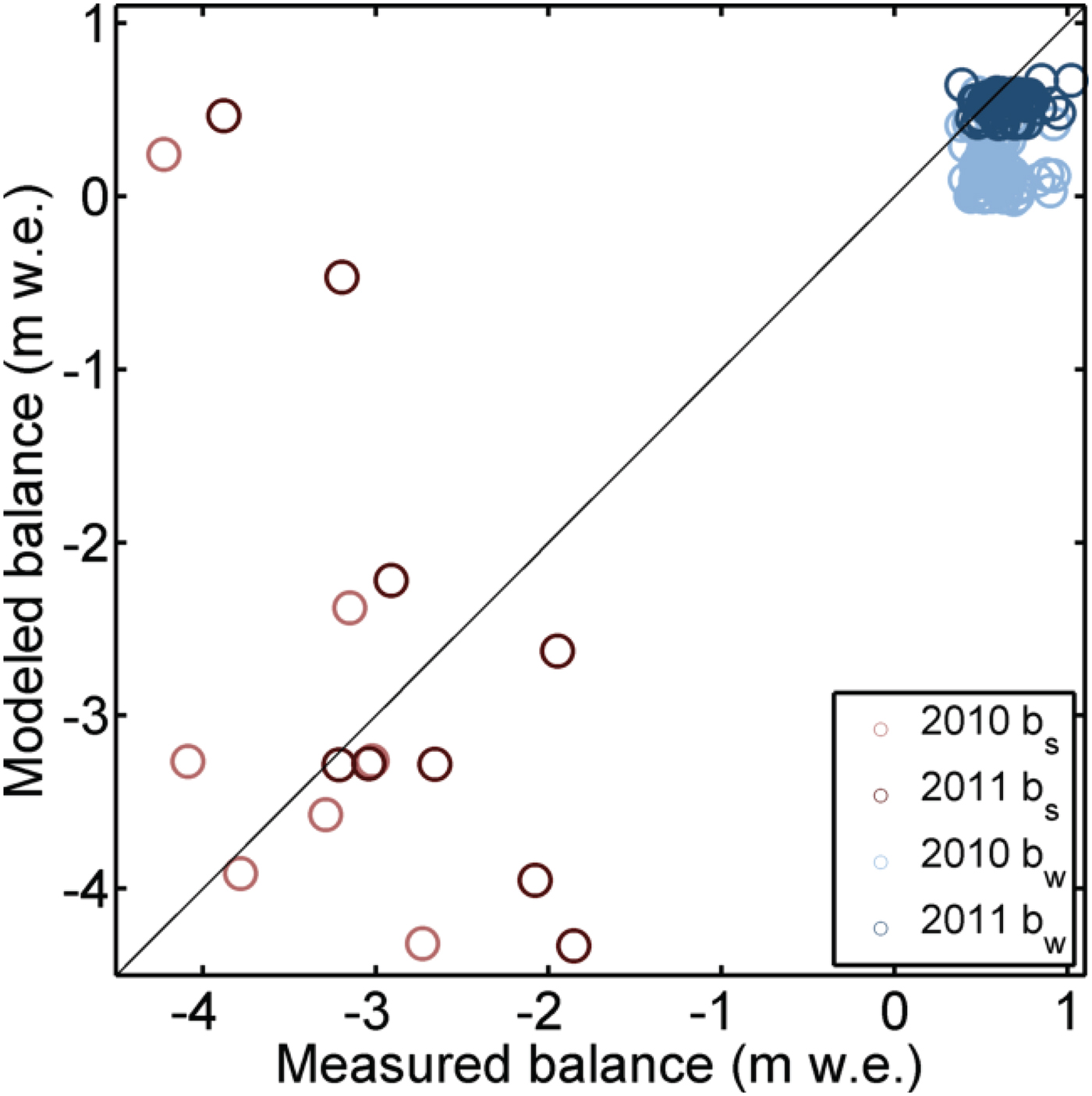
Fig. 6. Modeled and measured summer and winter point mass balances for the single best-performing parameter combination of all model simulations (RMSE = 0.57, B = − 0.73 m w.e. a−1, with parameter values F m = 4.9 d−1 °C−1, a ice = 0.0012 mm m2W−1d−1 °C−1, a snow = 0.0011 mm m2W−1d−1 °C−1, F deb = 1.0, p grad = 0.57 mm w.e. (100 m)−1, and p corr = 432%).
Finally, we provide independent validation of our model findings by comparing our cumulative mass-balance time series against the spatially downscaled GRACE time series for the overlapping period (Jan 2003–June 2014). We detrend both time series to remove long-term mass loss trends before performing linear regression, in order to examine the correlation of interannual mass fluctuations.
5. RESULTS
We reconstruct the mass-balance evolution of the Kahiltna Glacier for 1991 to 2014, yielding a mean net mass-balance rate of −0.74 m w.e. a−1 (σ = 0.04 m w.e. a−1, referring to the std dev.of the 17 best-performing model simulations) as calibrated to laser altimetry estimates and point mass-balance observations. Figure 7 shows the suite of cumulative mass-balance time series generated by simulations with best-performing parameter combinations. It also shows the cumulative mass-balance time series from GRACE, beginning in early 2003. The y-axis starting value of GRACE is chosen as the mean of the 17 model simulations at the corresponding date, for the sake of visually comparing the time series. In performing linear regression of the detrended GRACE estimates to the detrended modeled time series for the overlapping 2003–2014 time period at the ~30-day GRACE time step, we find significant correlation between the two time series (R 2 = 0.58 and p ≪ 0.001), serving as validation of our calibrated model results with respect to accurately capturing interannual variability.
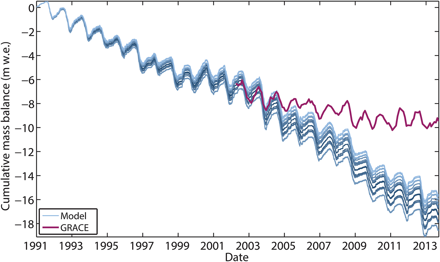
Fig. 7. Modeled cumulative daily glacier-wide specific mass balance (B) of 17 best-performing parameter combinations ( $\dot {B}$
within ± 10% of target value −0.73 m w.e. a−1 for 1994 to 2013 and RMSE ≤ 0.05RMSEmin), shown in shades of blue. Cumulative monthly mass balance from GRACE is shown in purple beginning on its launch date, with the y-axis starting value chosen as the mean of the 17 model simulations for the corresponding date, for the sake of visual comparison. Note that the GRACE time series represents specific cumulative mass balance for all glacier ice within the Central Alaska Range mascon, as opposed to the Kahiltna Glacier alone.
$\dot {B}$
within ± 10% of target value −0.73 m w.e. a−1 for 1994 to 2013 and RMSE ≤ 0.05RMSEmin), shown in shades of blue. Cumulative monthly mass balance from GRACE is shown in purple beginning on its launch date, with the y-axis starting value chosen as the mean of the 17 model simulations for the corresponding date, for the sake of visual comparison. Note that the GRACE time series represents specific cumulative mass balance for all glacier ice within the Central Alaska Range mascon, as opposed to the Kahiltna Glacier alone.
Figure 8 further compares mass-balance estimates from our model simulations and GRACE, broken down into seasonal (winter and summer) and annual balances. Balance years begin during the fall of the previous year, and for GRACE represent the difference between successive maxima and minima in the full time series shown from Figure 7. While correlation is not significant between GRACE-derived and model-derived winter balances (R 2 = 0.02 and p = 0.73), it is strong for summer (R 2 = 0.69 and p = 0.003) and annual balances (R 2 = 0.63 and p = 0.006). Mean winter, summer, and annual balances from GRACE are respectively 1.27 (σ = 0.30, referring to std dev. of annual variability), −1.48 (σ = 0.45), and −0.21 (σ = 0.50) m w.e. for the 2003 to 2014 period, as compared with mean modeled estimates of 0.67 (σ = 0.32), −1.65(σ = 0.50) and −0.99(σ = 0.57) m w.e.
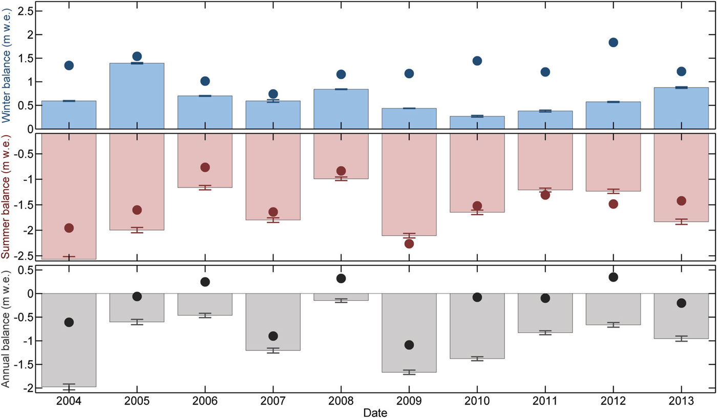
Fig. 8. Comparison of stratigraphic seasonal and annual balances from GRACE (points) and our model simulations (bars). For the modeled estimates, balances are averaged from the 17 best-performing model simulations ( $\dot {B}$
within ±10% of target value −0.73 m w.e. a−1 for 1994–2013 and RMSE ≤ 0.05RMSEmin). Whiskers indicate ± one std dev. from the mean of the 17 modeled estimates. Balance years begin during the fall of the previous calendar year.
$\dot {B}$
within ±10% of target value −0.73 m w.e. a−1 for 1994–2013 and RMSE ≤ 0.05RMSEmin). Whiskers indicate ± one std dev. from the mean of the 17 modeled estimates. Balance years begin during the fall of the previous calendar year.
In Figure 9, we show the time series of measured annual balances at the NPS index site location compared with modeled annual estimates for both (a) that same point location, and (b) the full glacier (i.e. glacier-wide balance). All three time series show balances for identical floating date time periods – that is, both modeled index site point and glacier-wide balances represent the mass-balance differences between that NPS observation date and the previous date, as extracted from the full model simulations. Correlations between the annual observed index site balances to either modeled quantity are weak: between the modeled and measured index site point balances, we find R 2 = 0.12 and p = 0.11, and between the modeled glacier-wide and observed index site, we find R 2 = 0.22 and p = 0.03.
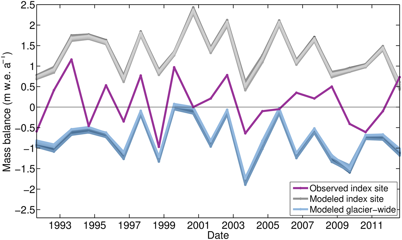
Fig. 9. Modeled and observed annual point balance at the NPS index site from 1991 to 2014, as well as modeled annual glacier-wide balance. All three time series refer to the floating date time system, as both modeled index site point and modeled glacier-wide balances are extracted from the full model simulations at exactly the NPS observation dates.
Overall, calibrated model simulations are validated by significant correlation with the full ~30-day mass change time series from GRACE, but correlate poorly with the NPS long-term record of point mass-balance observations at a single-stake index site.
6. DISCUSSION
Our study finds the 1991–2014 mean annual mass-balance rate for the Kahiltna Glacier to be −0.74 mw .e.a−1 (σ = 0.04 m w.e. a−1, referring to the std dev. of the 17 best-performing model simulations), with mean winter and summer balances of 0.72 m w.e. (σ = 0.06 m w.e.), and −1.51 m w.e. (σ = 0.20). These modeling results align reasonably well with findings for the same time period from the nearest monitored glaciers in the Alaska Range, namely Black Rapids Glacier and the Gulkana Glacier, respectively, situated ~280 and 300 km east-northeast of the Kahiltna. Black Rapids Glacier is estimated to have mean annual, winter, and summer balances of −0.57 m w.e., 1.01 m w.e. and −1.57 m w.e. for 1991–2014, based on modeling simulations calibrated to in situ and remotely sensed data (Kienholz and others, Reference Kienholz, Hock, Truffer, Bieniek and Lader2017). Annual, winter, and summer balances for the Gulkana Glacier, a USGS benchmark glacier originally selected to be representative of all glaciers within the region, are estimated to be −0.75 m w.e., 1.21 m w.e., and −1.97 m w.e., as derived by integrating field observations over a routinely updated glacier hypsometry (Van Beusekom and others, Reference Van Beusekom, O'Neel, March, Sass and Cox2010; O'Neel and others, Reference O'Neel, Hood, Arendt and Sass2014). Of noteworthy similarity are the summer balances for the Kahiltna and Black Rapids glaciers, and the annual balances for the Kahiltna and Gulkana glaciers, despite the distance between them and differences in size and geometry. It is not known whether discrepancies in mean winter balances of all three glaciers are due to true differences in climatic regime across the Alaska Range or due to the difficulty of accurately characterizing snowfall in these regions.
In reconstructing the 1991–2014 mass balance of the Kahiltna Glacier, our greatest challenges are the limited availability of both constraining mass-balance data across the >5800 m elevation range, and climate data products that accurately capture high-elevation conditions. Due to difficulty of access, we do not have any measurements of snow accumulation on the Kahiltna Glacier at elevations > 2340 m a.s.l., and our lower elevation (800–1400 m a.s.l.) measurements have high snow depth and summer melt variability due to considerable ice surface topography. In terms of climate data, the only long-term and continuous observational weather station data available for the area are 60 km distant from the glacier, well outside of the Central Alaska Range topography. The noteworthy scarcity of high-elevation weather station records in Alaska is a well-known problem for accurately characterizing climate patterns (Bieniek and others, Reference Bieniek2012). Moreover, reanalysis climate products available for the region, including NCEP–NCAR, typically have coarse resolution that neither represents the complex topography of Alaska mountain ranges nor includes high-elevation weather station data (Lader and others, Reference Lader, Bhatt, Walsh, Rupp and Bieniek2016). Together, these issues help explain our difficulty in reproducing point mass-balance observations and their associated balance gradients with our mass-balance modeling, as was also the case for recent modeling studies on Yakutat Glacier and the Juneau Icefield, both in Alaska (Trüssel and others, Reference Trüssel2015; Ziemen and others, Reference Ziemen2016). These challenges help us frame our discussion for monitoring recommendations for the future.
6.1. GRACE
Correlation between the full time series of detrended GRACE and detrended modeled estimates of mass change for the overlapping 2003–2014 time period is significant (R 2 = 0.58 and p ≪ 0.001). This suggests that both GRACE and our model simulations are capturing the same climate processes driving interannual mass changes. In comparing seasonal and annual balances, although correlation is poor between GRACE-derived and model-derived winter balances (R 2 = 0.02 and p = 0.73), it is noteworthy in its strength for summer (R 2 = 0.69 and p = 0.003) and annual balances (R 2 = 0.63 and p = 0.006). The strong annual correlation despite the low winter correlation supports the concept that mass-balance variability of continental glaciers like the Kahiltna is primarily controlled by summer temperature rather than winter precipitation (Arendt and others, Reference Arendt, Walsh and Harrison2009; Cuffey and Paterson, Reference Cuffey and Paterson2010; O'Neel and others, Reference O'Neel, Hood, Arendt and Sass2014).
The poor correlation between modeled and GRACE-derived winter balances could be due to uncertainties in our model and/or uncertainties in GRACE observations. In terms of uncertainties in the model, one possible explanation for the discrepancy is due to problems with accurate characterization of precipitation processes, with respect to both climate data input and constraining data, which are especially lacking at high elevations. Regarding uncertainties in GRACE, the two primary considerations are signal magnitude and signal attribution. Signal magnitude can be in error if significant mass leakage occurs between mascons. However, this problem would then cause poor summer balance correlations as well, which we do not see. In terms of attribution, although the GRACE solution we use does attempt to forward-model and remove terrestrial water changes, previous work shows that isolating mass changes from glacierized versus nonglacierized terrain is challenging (Lenaerts and others, Reference Lenaerts2013; Beamer and others, Reference Beamer, Hill, Arendt and Liston2016). Although this is an issue when comparing mass-balance magnitudes, because seasonal snowpacks tend to have similar phases of variability on- and off-glacier, this problem should have minimal impact on our model/GRACE comparisons that only examine correlations in seasonal variability. For example, Figure 8 in Beamer and others (Reference Beamer, Hill, Arendt and Liston2016), a study that examines freshwater discharge into the Gulf of Alaska by comparing model results to GRACE, shows that regional mass changes have very similar shapes for both ice and ice + land signals. Overall, we think it is unlikely that seasonal patterns in snow accumulation and ablation are vastly different on and off ice in our domain of study, and therefore attribute the majority of the disagreement to our model, which is poorly constrained with respect to snow accumulation.
In the long term, GRACE shows a less negative mass-balance rate than those from the model simulations, at −0.25 m w.e. a−1 for 2003–2014 (compared with −0.93 m w.e. a−1 for the same period from the model). This discrepancy is likely due to signal leakage between adjacent mascons that is inherent in GRACE processing (Arendt and others, Reference Arendt2008; Luthcke and others, Reference Luthcke2013), which would reduce the amount of mass loss that should be attributed to the highly glacierized Alaska Range by distributing it in part to surrounding areas. As such, we suggest GRACE is not yet suitable for deriving long-term trends at the mascon scale without first applying additional constraints in the GRACE-processing chain. Nonetheless, we take our results in comparing GRACE to modeled estimates to indicate that GRACE is a useful validation tool when modeling sub- and interannual mass changes for individual large glaciers, and may one day itself be a promising tool for reconstruction studies on its own.
6.2. Single-stake method
The single-stake method assumes that for a site located near the glacier's long-term ELA, mass balance should be zero most years or should otherwise fluctuate in response to positive or negative balance years, therefore serving as a good indicator of glacier-wide balance (Ohmura and others, Reference Ohmura, Kasser and Funk1992; Mayo, Reference Mayo2001). However, the success of the method relies on the chosen site being representative of more than localized conditions at that point.
Due to low correlation with our modeled results, we conclude that mass balances at the single NPS index stake do not accurately represent glacier-wide balances. This is in contrast to the previous work by Rasmussen (Reference Rasmussen2004), which examined the elevation dependence of annual point balance on 12 small (<73 km2) glaciers in Scandinavia to show an example of a region where a single stake works remarkably well. The glaciers included in that study exhibited a highly linear slope of net balance with elevation (i.e. balance gradient) that remained constant in time, even if the elevations or balances themselves shifted. High correlation between net balances for multiple glaciers also meant that measurements on one glacier served as a reasonable predictor of other glaciers in the region. The authors attributed the result to unique local climatic and topographic controls, including low topographical relief.
We suggest that while the single-stake method is not appropriate for the Kahiltna Glacier with its large elevation range, it may be appropriate for smaller glaciers with less point-to-point variability, or for glaciers with well-known balance gradients over the full elevation range. On the Kahiltna, it is likely that observed index site point balances are predominantly sensitive to the position of the stake within valleys and troughs of the local ice surface topography as opposed to the climatologically driven processes of model simulations. We also note that processes around the ELA may contribute to a particularly sensitive b index, as a balance at this location is near-zero and therefore susceptible to small mass changes of snow versus ice that may not match the glacier-wide changes from modeling results.
Where single stakes are insufficient, it is possible to instead identify the minimum number of stakes needed to capture temporally invariant balance gradients. Fountain and Vecchia (Reference Fountain and Vecchia1999) discovered that for two small (2.90 and 0.20 km2) glaciers with an extensive measurement record, reducing a larger stake network to between 5 and 10 stakes over each glacier's elevation range had little effect on glacier-wide mass-balance uncertainty. This minimum of 5–10 stakes agrees with both Funk and others (Reference Funk, Morelli and Stahel1997), who reduced their stake network to six for a small (6.20 km2) Swiss glacier after an initial elevation-dependent balance function was determined, and with Cogley (Reference Cogley1999), whose statistical study confirmed that dense networks of point mass balance are probably not necessary, as stakes close in elevation are highly correlated. However, Fountain and Vecchia (Reference Fountain and Vecchia1999) argued that there must be an upper limit to the scale invariance of the findings in Cogley (Reference Cogley1999), particularly since large glaciers are exposed to different climates, such that their mass balance with elevation relationship may change several times. Given the Kahiltna Glacier's >5800 m altitudinal range and location among prominent weather-creating peaks such as Denali, changes in climatic regime with elevation are highly likely. We therefore emphasize the need for any stake network to cover as much of the elevation range as possible. However, if a single-location method is the only feasible approach for a glacier with a large elevation range, we recommend at least deploying several stakes near the ELA to sample different local conditions and averaging these.
6.3. Multi-method monitoring recommendations
Glaciers with altitudinal ranges large enough to experience different climatic regimes with elevation, a situation that is likely a function of local topography and climatic conditions more so than a specific altitudinal threshold, require special consideration in mass-balance monitoring. Overall, we can make several recommendations for improving monitoring approaches for these glaciers based on our results, and based on the success of other multi-method modeling approaches pioneered in an earlier work (Huss and others, Reference Huss, Bauder, Funk and Hock2008).
A principal issue is that for the Kahiltna Glacier, due to its altitudinal range, spatial distribution of precipitation remains largely unknown. Initial model simulations revealed that the PRISM gridded climate product attributed too steep a precipitation gradient over lower portions of the glacier (47.30 mm w.e. (100 m)−1) and a rainshadow at 1925 m a.s.l., though we have no observational evidence to either confirm or deny this. Best-performing parameter combinations yielded a precipitation gradient of 5.70 mm w.e. (100 m)−1 to 19.60 mm w.e. (100 m)−1 for elevations to 1925 m a.s.l. In this respect, Kahiltna appears to be an outlier to Figure 7 in the study by McGrath and others (Reference McGrath2015) who, from helicopter-borne ground-penetrating radar (GPR) campaigns of snow depth and snow water equivalent elevational profiles of several Alaska glaciers, proposed that precipitation gradients could be approximated as a linear function of distance from the coast. Moreover, as evidenced by our ground observations, NCEP–NCAR climate data for the area underestimated precipitation on the Kahiltna Glacier by nearly 400% at the elevation of our AWS. In these ways, our knowledge of snow distribution and magnitudes on the glacier are currently quite limited. This problem likely extends to other glaciers covering extreme altitudinal ranges, due to the inherent difficulty of measuring snowfall at high elevations.
Recent studies on Alaska glaciers have revealed the importance of summer balance as the dominant control over long-term mass loss, driven by an overall increasing trend in summer air temperatures (Rasmussen, Reference Rasmussen2004; Arendt and others, Reference Arendt, Walsh and Harrison2009; O'Neel and others, Reference O'Neel, Hood, Arendt and Sass2014; Larsen and others, Reference Larsen2015). Our findings demonstrate that although summer balances do dominate long-term mass changes, winter balances dominate our current uncertainty in those estimates. This is in line with Huss and Hock (Reference Huss and Hock2015), who point out in their global climate model-driven projections for global glaciers that the wide range of outcomes of volume loss to 2100 are predominantly due to uncertainty about precipitation input.
To resolve this, we recommend a campaign of GPR to measure snow depth along the full glacier centerline near the end-of-winter maximum, in order to characterize precipitation gradients along the full elevation range. It may be possible from these data to identify a threshold elevation above which the gradient stabilizes, and below which the high level of snow depth variability due to ice surface topography on the large ablation area may be constrained. Ground truthing observations along this profile would be necessary, in order to correctly characterize snow water equivalent values. Because our bulk density values from vertical profiles in snow pits are consistent at different locations throughout our visited elevation range (n = 5), it can be argued that depth measurements may be more important than density in these field observations.
Any continued modeling efforts will also need to account for possible changes in ablation gradient over time, which would therefore require occasional installation of multiple ablation stakes at several elevations. Because of the high degree of ice surface topography seen in the ablation zones of large glaciers such as the Kahiltna, if monitoring priorities are budget-limited, it would be recommended to at least place several stakes at each elevation visited in order to better constrain ablation variability at any one location/elevation. Moreover, continued modeling will also need to adjust for changing glacier geometry (i.e. primarily elevation changes) over time, as the glacier continues to thin.
We also underscore the importance for ongoing modeling efforts of relying on more than just point mass balances for calibration, by making use of a glacier-wide geodetic mass-balance constraint, such as from laser altimetry or DEM differencing approaches. Had we calibrated to point mass-balance measurements alone and not included a primary constraint from laser altimetry, our long-term mass-balance estimates would have extended across a range from −0.12 to 0.56 m w.e. a−1, with a mean value of 0.26 m w.e. a−1 (σ = 0.18 m w.e. a−1) for the period from 1991 to 2014. This is a noteworthy discrepancy from the laser altimetry-constrained value of −0.74 m w.e. a−1 (σ = 0.04 m w.e. a−1). Nonetheless, the true advantage comes from using geodetic estimates and mass-balance modeling together, as geodetic estimates alone represent only bulk changes and provide no information about sub- or interannual mass variations.
Ultimately, the data collection and methods used will be a balance between data coverage and efficiency of analysis versus feasibility and cost of acquiring quality data, and will be dictated by the goals of the monitoring program. In the case that long-term mass changes are of interest, geodetic balances such as those acquired from laser altimetry are the most reliable tools for large glaciers. If seasonal and interannual mass changes are also of interest, a combination of modeling tools constrained not only to stake measurements but also to geodetic estimates are recommended, and validation against products such as GRACE can yield greater confidence in results. Our recommendation for glaciers with extreme elevation ranges based on this study is a monitoring approach that employs a stake network covering as large an elevation range as is reasonably possible, that better characterizes winter precipitation by GPR snow radar profiling, and that leverages available geodetic data to better estimate mass changes at both seasonal and longer-term time scales.
7. CONCLUSIONS
Combining enhanced temperature index modeling with new ground observations and laser altimetry estimates, and validating against a simple spatially downscaled GRACE gravimetry solution, we reconstruct the mass-balance evolution of the Kahiltna Glacier for 1991 to 2014, finding a mass-balance rate of −0.74 m w.e. a−1 (σ = 0.04 m w.e. a−1, std dev. of the 17 best-performing model simulations).
We find that this site is a challenge for a traditional approach using an enhanced temperature index melt model alone. In terms of climate forcing data, we lack a long-term continuous observational weather station record within 60 km of the glacier, and reanalysis climate products for the region have coarse resolution that neither captures the complex topography of the area nor incorporates high-elevation station data into its product. This is especially problematic for characterizing precipitation across the full elevation range, and our model yields winter mass-balance results that are incongruous with our GRACE gravimetry validation dataset.
We also find that modeling simulations should not be calibrated to point mass-balance observations alone, particularly given a lack of constraining snow water equivalent data, which is both sparse over the elevation range and highly variable. If we did not incorporate laser altimetry estimates as a primary calibration constraint, model simulations optimized only to point mass-balance measurements would yield long-term estimates ranging from −0.12 to 0.56 m w.e. a−1, with a mean value of 0.26 m w.e. a−1 (σ = 0.18 m w.e. a−1), for the period from 1991 to 2014.
Detrended GRACE gravity estimates of mass change between 2003 and 2014 at the ~30-day GRACE time step correlate well (R 2 = 0.58 and p ≪ 0.001) with our modeled time series, suggesting that both GRACE and our model simulations are capturing the same climate-driven processes of interannual mass accumulation and ablation in the area. Moreover, while correlation is not significant between GRACE-derived and model-derived winter balances (R 2 = 0.02 and p = 0.73), it is strong for summer (R 2 = 0.69 and p = 0.003) and annual balances (R 2 = 0.63 and p = 0.006). This suggests that while winter accumulation processes continue to be the greatest uncertainty faced by mass-balance methods, GRACE is able to provide robust information on the variability of summer and annual mass changes. Summer balances for the 2003-2014 period also exhibit the smallest bias in terms of magnitude of the mean seasonal balances derived from GRACE (-1.48 m w.e., σ = 0.45) as compared with our modeled estimates (−1.65 m w.e., σ = 0.50). GRACE estimates also show a less negative long-term trend for the full time series than those from our laser altimetry-constrained model simulations (−0.24 versus −0.93 m w.e. a−1), which indicates that although our GRACE mascon solution version serves as a useful validation tool for evaluating subannual mass changes, it is not yet suitable for deriving long-term trends at the mascon scale without additional constraints applied in the GRACE processing chain.
We find low correlation (R 2 = 0.22 and p = 0.03) between our modeled time series of glacier-wide mass changes and a historic NPS point mass-balance record at a single index site near the ELA, suggesting that the single-stake index site is not effective at capturing glacier-wide interannual variations or long-term trends in mass change for this glacier, compared with our mixed method approach. A single index stake is highly subject to the location of its placement, given local variations in accumulation and ablation. As such, we suggest the single-stake approach is inadequate for glaciers with large altitudinal ranges over which there may be both changes in balance gradient with elevation as well as large point-to-point variability. However, if a single-location method is the only practical approach, we recommend deploying several stakes near the ELA to sample different local conditions and averaging these.
This study highlights the importance of incorporating multiple methods and datasets to help reduce uncertainty in mass-balance time series for glaciers with extreme altitudinal ranges, toward better understanding the response of these glaciers to a changing climate. Our approach may be widely applicable to similar glaciers in other regions of the world, particularly those with sparse spatial coverage of ground observations due to extreme topography and difficulty of access.
ACKNOWLEDGMENTS
The authors would like to thank Rob Burrows and Guy Adema of Denali National Park and Dr. Michael Loso of Alaska Pacific University for extensive field work support, which was carried out in Denali National Park under study #DENA-00810 and permit DENA-2010-SCI-0001. We also thank Talkeetna Air Taxi for logistical support, and Sam Herreid, John Hulth, Dr. Andreas Aschwanden and Dr. Alessio Gusmeroli for help in the field. Dr. Roman Motyka also contributed to earlier versions of this study. This work was funded in part by a George Melendez Wright Climate Change Fellowship and by the University of Alaska Fairbanks Center for Global Change/Cooperative Institute for Alaska Research. Arendt was supported by NASA's Cryospheric Sciences (NNX13AK37G) and GRACE science team (NNX16AF14G) programs. We also thank Dr. Dan Shugar and one other anonymous reviewer, whose insights greatly improved the manuscript.


 Open access