


Introduction
Knowledge of glacier ice volume is essential for the development of projections of glacier extent, sea-level rise and mountain hydrology. Since direct measurement of glacier volume requires extensive fieldwork, only a small fraction of the world’s glaciers and ice caps have been surveyed, and much work is being devoted to deriving methods to calculate current and future glacier volumes. Estimates of the present ice volume contained in mountain glaciers, provided by Reference Lemke and SolomonLemke and others (2007), differ considerably. Sea-level change corresponding to the different volume estimates ranges from 0.15 to 0.37 m.
Since the mid-1990s, the introduction of lightweight ground-penetrating radar (GPR) systems has allowed large-scale ground-based measurements of ice thickness on temperate alpine glaciers (e.g. Reference Narod and ClarkeNarod and Clarke, 1994). Airborne ice-thickness radar techniques have been used over mountain glaciers (e.g. Reference Macheret and ZhuravlevMacheret and Zhuravlev, 1982; Reference Dowdeswell, Drewry, Liestøl and OrheimDowdeswell and others, 1984). Several different techniques may be used to estimate glacier volume from ice-thickness measurements. The simplest, but least accurate, is to estimate the total ice volume as the product of the glacier area and the average of the measured ice-thickness values. In order to derive the spatial distribution of the volume, either the ice-thickness or the bedrock elevation data are interpolated. The interpolation can involve additional information, such as topographic data and ice-dynamics considerations (e.g. Reference ErasovErasov, 1968; Reference BrücklBrückl, 1970; Reference Funk, Gudmundsson and HermannFunk and others, 1994; Reference Bauder, Funk and GudmundssonBauder and others, 2003; Reference Binder, Brückl, Roch, Behm, Schöner and HynekBinder and others, 2009). Reference LentnerLentner (1999), for example, determined the ice thickness of some Austrian glaciers by assuming elliptical-shaped glacier beds.
Based on glacier volume estimates derived from measured values of ice thickness, several empirical algorithms have been developed to calculate ice volume from easily observed ice surface quantities (e.g. Reference Driedger and KennardDriedger and Kennard, 1986; Reference Chen and OhmuraChen and Ohmura, 1990; Reference Meier and BahrMeier and Bahr, 1996; Reference TrabantTrabant, 1997). Reference Bahr, Meier and PeckhamBahr and others (1997) theoretically investigated a relationship between glacier surface area and volume and found that scaling factors can vary significantly (e.g. from one glacier to the other or on the same glacier under different conditions).
In order to add spatially distributed volume data to the Austrian glacier inventory (Reference Lambrecht and KuhnLambrecht and Kuhn, 2007), 53 glaciers were surveyed in 1995, 2006 and 2007 (Reference Span, Fischer, Kuhn, Massimo and ButschekSpan and others 2005; Reference Fischer, Span, Kuhn, Massimo and ButschekFischer and others, 2007) using GPR. In 1995, due to low computing and battery capacities and a limited project and time budget, the density of measurements per glacier was sparse. Ice thickness was measured along several profiles on each glacier. A sketch of a typical spatial distribution of samples is shown in Figure 1. On average, ice thickness was measured at a density of 33 points per km2, ranging from 7 to 220 points per km2 depending on the size of the glacier and complexity of the terrain. In very steep, crevassed, avalanche- or ice-/rockfall-affected areas, no measurements were carried out. Surveyed glaciers included large valley glaciers as well as small, flat cirque glaciers and steep, crevassed glaciers of medium size. As much as possible, we calculated glacier volume using the same technique for every glacier in order to obtain a homogeneous dataset. Since the spatial resolution of GPR measurements varied, it seemed most practical to construct the bedrock manually, based on the measured values of ice thickness and the topographic data of the 1998 Austrian glacier inventory. This method is demonstrated for Schaufelferner, Stubai Alps. In addition to the sparse data acquired early in the campaign, GPR data with higher spatial resolution were acquired in 2003 and 2006. These are used to estimate the accuracy of ice volume calculated from the sparse data. Different scaling algorithms and automatic gridding of the bottom topography data were also used to calculate the volume of Schaufelferner. The volumes are compared and set in relation to recent ice-thickness changes in order to decide whether the accuracy is at least in the same order of magnitude as the thickness changes.

Fig. 1. Typical spatial distribution of ice-thickness measurements on Austrian glaciers during the GPR campaigns of 1995–2007
Schaufelferner had an area of 1.4 km2 in 1997 and covered elevations between 3200 and 2700 m. The orthoimage and elevation contours (1997) are shown in Figure 2. In recent years, very few crevasses have been observed since the flow velocities have decreased (personal communication from W. Müller, 2005). The glacier is exposed to the north and has a low surface slope. On Schaufelferner, several independent campaigns measuring ice thickness have been carried out. Locations where GPR data were acquired in 1995, 2003 and 2006 are shown in Figure 2. Between 2005 and 2008, repeat measurements were performed to investigate temporal changes and the accuracy of the system. The location of these repeat measurements is indicated in Figure 2. Digital elevation models (DEMs) of Schaufelferner were acquired from airborne photogrammetry in 1969 (Reference PatzeltPatzelt, 1980) and 1997 (Reference Lambrecht and KuhnLambrecht and Kuhn, 2007) and airborne laser scanning in 2006 (Government of Tyrol). All DEMs use the Austrian Gauss–Krüger system.

Fig. 2. Orthoimage contours of elevation in 1997 and glacier area in 1969, 1997 and 2006 for Schaufelferner, Stubai Alps. The locations of the ice-thickness measurements during the 1995, 2003 and 2006 campaigns and the repeat measurements in 2008 are indicated.
Methods
Radar equipment
The data were collected using the miniature high-power impulse transmitter developed by Reference Narod and ClarkeNarod and Clarke (1994). Until 1998, the signal was received with an oscilloscope card in a notebook computer. After 1998, a Fluke 105B oscilloscope was used as receiver. The dipole antennas with non-reflecting resistive loading (Reference Wu and KingWu and King, 1965; Reference Rose and VickersRose and Vickers, 1974) were built in-house. Corresponding to the antenna half-lengths, l, of 15 and 25 m, the central frequencies, f c, are 6.4 and 3.8 MHz respectively according to
(personal communication from B. Narod, 1996). The centre-to-centre separation, a, of the antennas was equal to the antenna half-length during most field campaigns. The ice thickness was calculated from the measured time difference, Δt, between travel time of the signal transmitted through the air, t a, and the signal reflected from the ground, t r (Fig. 3).

Fig. 3. Measurement geometry assumed for calculating ice thickness.
The propagation velocity was not determined at the measurement locations but was assumed to be 168 m μs−1 (Reference Narod and ClarkeNarod and Clarke, 1994; Reference BauderBauder, 2001). This value is well within the range given in the literature (e.g. 167.7 m μs−1 (Reference Glen and ParenGlen and Paren, 1975); 168.5 m μs−1 (Reference RobinRobin, 1975); 169.0 m μs−1 (Reference Kovacs, Gow and MoreyKovacs and others, 1995)). The path of the reflected signal has length s, where
with t r travel time and c i the velocity of the signal in the ice.
Assuming a locally homogeneous plane-parallel ice block, the ice thickness, h, is given by
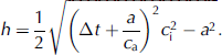
This equation is based on a geometric setting as indicated in Figure 3.
Data acquisition
The GPR data on Austrian glaciers are ground-based, acquired mainly during the late winter months. The locations of measurements on the glacier surface were determined with an average accuracy of ∼10 m horizontally using a Garmin Summit global positioning system (GPS). The number of measurements is limited by the time and effort required in the field and for data processing, especially in the early years of the measurements when power supply was limited. Measurements are not located in a regular grid but on profiles along and across the glacier. During the earlier GPR surveys of Austrian glaciers, measurements were carried out with the aim of finding a maximum ice-thickness value on each glacier. Thus, the deepest location in a cross-profile was chosen as the starting point for a longitudinal profile. The focus on maximum ice thickness has the advantage that misinterpretation of ice thickness caused by bedrock undulations in the order of magnitude of ice thickness plays no role. After 2003, areas with shallow ice cover were also investigated and mapped, since these areas are important for the development of projections of glacier area. On average, the ice thickness was measured at 33 locations per km2. The GPR 1995 data of Schaufelferner can be considered ‘typical’ for the above-described data samples.
Accuracy of ice-thickness measurements
The accuracy of ice-thickness estimations from GPR measurements is determined by two factors: the accuracy of the measurement system and the properties of the ice and bedrock. For the first the resulting errors are small compared to the measured values. Depending on the scale used to display the data, the run time of the signal can be measured with an accuracy of ±30 ns. Four antennas are used, arranged in two pairs. The antennas coupled to the receiver are positioned parallel to the antennas coupled to the sender. Because of glacier surface undulations, we sometimes know the distance between antenna pairs to an accuracy of only ±2 m. For a typical run time of 1 μs the resulting accuracy of the calculated ice thickness is ∼±3 m.
The second source of error is more difficult to quantify and can have far larger effects on the estimation of ice thickness. The internal structure of the glacier, including crevasses, internal boundaries and inhomogeneities, as well as topography and roughness of the bedrock, can cause large errors. In the case of multiple reflections, identification of the signal reflected from the bedrock can be difficult or even impossible. Bedrock undulations on the same order of magnitude as the ice thickness can lead to misinterpretation of the data.
We assume the glacier ice to be homogeneous, and firn layers and seasonal snow cover at the time of the measurement are neglected. Errors due to winter snow cover are expected to be smaller than ±5 m, and in most areas even lower. Sparse information on the thickness of firn layers on Austrian glaciers is available. From a firn pit on Kesselwandferner, Ötztal Alps, in the 1970s (Reference AmbachAmbach and others, 1978, Reference Ambach, Huber, Eisner and Schneider1995) it is estimated that the thickness of firn layers today varies between 0 and ∼20 m. Reference Haeberli, Wächter, Schmid and SidlerHaeberli and others (1982) estimated the error introduced by neglecting firn layers at ∼5%. A short calculation using Equations (2) and (3) demonstrates the possible effect of neglecting firn layers, which causes an underestimation of ice thickness, and winter snow layers, which causes an overestimation of ice thickness. Assuming a signal velocity of 200 m μs−1 in firn and 290 m μs−1 in dry winter snow, the effects of neglecting a winter snow cover of 4 m and a firn layer of 30 m thickness compensate each other.
Maps and photos were used to determine larger-scale bedrock undulations, since ridges in the bedrock are often indicated by crevasse zones. We conclude that a good estimate for the measurement uncertainty of typical thicknesses (30–300 m) of Austrian glaciers will be in the order of 5–10% of the measured value. Single points exhibiting unfavourable geometry can show far larger deviations, also affecting the total glacier volume. Therefore the data were carefully controlled and the spatial interpolation was based on manually constructed contours of ice thickness. In very steep and/or crevassed areas, no measurements were carried out.
Volume Calculation
Since the method for determining the spatial distribution of ice volume is applied to a finite number of completely different types of glaciers with different sample density, the bedrock topography was constructed manually according to the measured ice-thickness and glacier inventory data. Glaciers with large crevasse zones especially exhibit sparse and not well-distributed ice-thickness data. A supervised method reduces the need to fill data gaps, as it becomes necessary for an automatic algorithm to be applied. Filling the data gaps by educated guess or automatic procedures involving ice dynamics creates at least two different categories of volume datasets without totally excluding subjective decisions.
The Austrian glacier inventory includes the glacier margins and DEMs of all Austrian glaciers between 1997 and 2002. At each GPR measurement position, the ice thickness was subtracted from the surface elevation from the glacier inventory DEM. The surface-altitude changes between the dates of the radar survey and the acquisition of the DEMs are within several meters. Figure 4 shows the change in surface elevation of Schaufelferner between 1997 and 2006.

Fig. 4. Maps of ice-thickness change from 1969 to 1997 (a) and from 1997 to 2006 (b), calculated from the DEMs.
Contours, at 20 m spacing, of bed topography were constructed according to the assumptions:
at the margin of the glaciers, including nunataks and rock outcrops, the ice thickness is zero.
the slope of periglacial rocks, but not debris near and under the ice, is approximately the same.
the ice thickness in crevassed zones is lower than in nearby areas exhibiting the same surface slope but no crevasses.
A bed topography for Schaufelferner was constructed based on the 1995 GPR measurements. The interpolation of the contours to calculate a raster format DEM of the bed topography was carried out in ArcGIS 9.3 using the Topo2Raster tool, which is based on the ANUDEM algorithm (Reference HutchinsonHutchinson, 1989; Reference Hutchinson and DowlingHutchinson and Dowling, 1991). The method uses iterative finite-difference interpolation, which was designed to do ‘intelligent interpolation’ preserving natural structures such as drainage systems, ridges and hilltops. This algorithm allows inclusion, not only of contour input data, but also of point elevations and margins where the user can define the priority of different types of input data.
Applying Topo2Raster to the contours of bed topography and glacier margins, the total volume was found to be 0.043 km2, corresponding to an average ice thickness of about 30 m (Table 1). The 40 m contours of bed topography and the spatial distribution of ice thickness are shown in Figure 5 (GPR 1995 c; Table 1).
Table 1. Volume (km3) of Schaufelferner calculated from measured data and scaling algorithms for 1997. The volumes for 1969 and 2006 are calculated by subtracting the volume differences from the DEMs of 1969, 1997 and 2006 from the 1997 volume. The areas given (km2) are used to calculate the mean ice thickness (Fig. 8)


Fig. 5. Contours of bed topography (a) and calculated map of ice thickness (b) based on the GPR 1995 data.
On the Accuracy of the Volume Determination
Before volume data can be used in further investigations of glacier change, we need to know the magnitude of the volume error bar and the certainty of the spatial distribution of the ice mass. The requirements on the accuracy of the volume data, of course, depend on the type of investigation, but a good starting point is a comparison with average thickness changes on a timescale of, for example, a decade. The average ice thickness of Austrian glaciers has reduced by 1 m a−1, averaged over the total glacier surface over the past three decades (Reference Lambrecht and KuhnLambrecht and Kuhn, 2007). This is of the same order of magnitude as the accuracy of a single ice-thickness measurement by GPR. To meet the requirement that decadal changes in ice thickness are resolved in the volume data, the accuracy of the ice volume should allow the calculation of the mean ice thickness with an accuracy of ∼10 m. Therefore, the accuracy of the volume should be 10 m3 per m2 of glacier area in order to allow an interpretation of glacier volume changes.
If the ice-thickness measurements were distributed over the glacier on a regular grid, the mean ice thickness could be calculated as the average of the measured values, and the volume error bars would be directly related to the accuracy of the ice-thickness measurements. This is not the case, so the accuracy of the ice-thickness data does not give us any clue on the accuracy of the total volume. Assuming that a GPR measurement is representative of the ice thickness within a square of 100 m × 100 m, the 36 GPR measurements from 1995 will cover 25% of the area of Schaufelferner.
The completely independent GPR data of 2003/06 include 144 ice-thickness measurements which, on the above assumption, cover 100% of the area of Schaufelferner. These data were used to derive a volume which can be considered to be closer to reality. The deviation from this more realistic volume can be considered as the error bar on the 1995 volume estimation. In order to obtain a more reliable estimate of the variability of volumes derived from measurements, different methods were used for the volume determination, including automatic gridding. This resulted in an ice-thickness grid, which made it possible to compare not only the total volume, but also the ice-thickness distribution.
Additionally, the total volume was calculated using various scaling methods. The bandwidth of these estimates should give an indication of the degree to which results for an individual glacier can differ.
Comparing Spatial Distributions of Ice Thickness
An automatic gridding was applied to the 1995 GPR data (GPR 1995 p, Table 1; Fig. 6a). For the unsupervised interpolation of the sparse data, the kriging algorithm is implemented in the ArcGIS 9.3 Spatial Analyst toolbox (e.g. Reference OliverOliver, 1990) was used. The ice thickness was taken to be zero at the margins, and a spherical semivariogram was assumed. From 144 ice-thickness measurements in 2003 and 2006, the volume was determined in the same way as above. The spatial distribution of the measurements and the topographic contours are shown in Figure 7. The contours were interpolated using the Topo2Raster tool, once based on contours and points (GPR 2003/06 cp; Table 1) and once based on contours only (GPR 2003/06 c; Table 1).

Fig. 6. (a-c) Maps of ice thickness calculated from (a) automatic gridding of GPR 1995 data; (b) interpolation based on contours of GPR 2003/06 data; and (c) interpolation of contours and points based on GPR 2003/06 data. (d) Map of differences in ice thickness between (b) and (c).

Fig. 7. Contours of bed topography based on the GPR 2003/06 data.
The maps of the ice-thickness distributions show high local differences in ice thickness (Fig. 6a–c). The maximum ice thickness of GPR 2003/06 c and GPR 2003/06 cp exceeds 100 m and is ∼30 m higher than for the GPR 1995 c data. The automatic gridding produces negative values of ice thickness in areas without measurements; the maximum ice thickness is similar to the GPR 1995 c data. The differences between the GPR 1995 c and the GPR 2003/06 c data are largest in areas where no 1995 measurements were performed. The GPR 2003/06 cp and the GPR 2003/06 c data differ in areas without measurements and near the glacier margins. The results at the locations of the GPR measurements are similar. Since including the point measurements in the Topo2Raster algorithm seems to introduce a higher gradient to the margins and valley-like structures along the GPR profiles, the GPR 2003/06 c volume is considered as the ‘true value’ in the following section. The local differences between the 1995 volume and the 2003/06 volume calculations (Fig. 6d) far exceed the ice-thickness change from 1997 to 2006 derived from the DEMs (Fig. 4).
Comparing Volumes
The volumes calculated from the 1995 GPR data show a larger dependency on the method applied, resulting in the highest (0.043 km3) and lowest (0.028 km3) volumes (Table 1). The GPR 2003/06 c (0.038 km3) and GPR 2003/06 cp (0.037 km3) volumes are much closer to each other. The accuracy of the volume for the GPR 1995 c data is estimated to be the difference from the volume GPR 2003/06 c which is ±0.005 km3 or ±12%.
The volume of Schaufelferner was also calculated according to Reference Müller, Caflisch and MüllerMüller and others (1976), Reference Macheret and ZhuravlevMacheret and Zhuravlev (1982), Reference Driedger and KennardDriedger and Kennard (1986), Reference Chen and OhmuraChen and Ohmura (1990) and Reference Bahr, Meier and PeckhamBahr and others (1997). These area–volume scaling algorithms were developed from, and possibly designed for, different volume data and are usually applied to a large sample of glaciers. Nevertheless, it might be of interest to compare the mean ice thickness calculated for one glacier with measured data. The mean ice thickness modelled by the area–volume scaling algorithms decreases by 0–4 m between 1969 and 1997 and 1–2 m between 1997 and 2006. This is much less than calculated from the difference from the 1969, 1997 and 2006 DEMs. According to those data, the mean ice thickness reduced by 8m between 1969 and 1997 and 5 m between 1997 and 2006. This is about twice the difference between the GPR 1995 c and GPR 2003/06 c mean ice-thickness values. So the requirement that multi-year ice-thickness changes be resolved is fulfilled for volumes calculated from measured values for the total glacier area. Locally the deviation of ice-thickness data can be higher. For the volumes calculated with scaling methods, the deviation from the ‘true’ value ranges from 3 to 32 m, with a mean of 14 m, about twice the ice-thickness change in the two periods.
The mean ice thicknesses of Schaufelferner calculated according to the volumes and areas given in Table 1 are shown in Figure 8. For 1997, the values of the mean ice thickness vary between 20 m (GPR 1995 p) and 62 m (calculated after Reference Macheret and ZhuravlevMacheret and Zhuravlev, 1982). The mean is 32 m, which is 5 m more than the ‘true’ GPR 2003/06 c value. The means of the measured ice-thickness values are among the highest estimates for the mean ice thickness. The volume of Schaufelferner was analyzed in a previous study by Reference LentnerLentner (1999) based on the data of 1995 and assuming an area of 1475 km2. The mean ice thickness she calculated, based on three part-volumes, was 3 m higher than the GPR 1995 c volume.

Fig. 8. Mean ice thickness for the volumes given in Table 1 for 1969, 1997 and 2006.
On the Determination of Volume Change by GPR
In order to investigate the potential of GPR for volume-change determination, repeat measurements were carried out on Schaufelferner. On one test site (AWS in Fig. 2), snow height and ice thickness were measured several times between 2003 and 2006 (Table 2). Between 2005 and 2008, the position of the antennas was determined with a differential GPS (DGPS) with an accuracy <1 m. In 2003, the position was determined with lower accuracy.
Table 2. Ice thickness and snow depth measured at AWS (Fig. 2) between 2003 and 2008

The antennas were oriented in the direction of the slope. The surface slope is about 5°, so the difference in surface elevation between the antenna ends is about 3 m. On 3 May 2005, the antennas additionally were turned by 90°, resulting in a decrease of 1 m in measured ice thickness. Between 2005 and 2008, the ice surface lowered by 7 m according to the DGPS measurements and 6 m according to the GPR data. According to the GPR measurements in 2005, the error of the ice thickness seems to be <1 m. Although the error in the positioning of the GPR is likely to be higher in 2003, with an estimated ice-thickness change of ∼3 m between 2003 and 2005, the measured ice thickness seems to have an accuracy of <3 m.
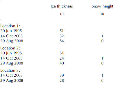
Three other locations (1, 2, 3 in Fig. 2) where the ice thickness was measured in 1995 and 2003 were revisited in 2008 (Table 3). Although the positions in 2008 were measured with DGPS, the ice thickness differs by up to 27 m. The DEMs of 1997 and 2006 show a surface lowering by 9–11 m at the location of the GPR measurements. These data indicate that the reliability of ice-thickness change data derived even with exactly the same GPR system is highly dependent on the reproducibility of the measurement location. If the geometry is changed by, for example, changes in the surface slope of the glacier or the beamwidth of the GPR system used, the errors might be high.
Table 3. Ice-thickness and (when available) snow-depth measurements for locations 1–3 (Fig. 2) between 1995 and 2008
Discussion and Outlook
The accuracy of glacier volume calculated from sparse 1995 GPR data and including topographic information from the Austrian glacier inventory was of the same order of magnitude as the multi-year volume change. So, in order to resolve multi-year volume change for 53 Austrian glaciers, the manual construction of ice thickness based on the glacier inventory and sparse GPR data is sufficient. The choice of method has a greater impact on the results of the spatial distribution of volume than on the total volume. The local differences in the ice volumes were tens of cubic meters per square meter of glacier area compared to a variability of a few cubic meters per square meter of glacier area (Table 1). For applications, where the spatial distribution of volume is important, the method for volume calculation has to be considered and described carefully. An increase in the spatial resolution of GPR measurements increases the accuracy of the spatial distribution of volume to a higher extent than the accuracy of the total volume.
Averaging the measured ice-thickness values overestimates the mean ice thickness of the glacier by up to 19 m, much more than the ice-thickness change on a decadal timescale. The grade of overestimation of the ice thickness is highly dependent on the choice of the location of the GPR measurements.
The volumes derived by volume–area scaling algorithms are, apart from one, within a range of ±5m for 1997. The application of these algorithms to the areas studied in 1969 and 2006 did not reproduce the measured volume changes between these years. A larger sample of glaciers will be investigated in a future project to find out whether the results for Schaufelferner are similar to those for other Austrian glaciers.
The accuracy of volume changes calculated from GPR measurements is highly dependent on the accuracy of the positioning. Therefore, the calculation of volume changes from surface elevation data seems to be a more cost-effective and accurate way of monitoring volume change. This is especially true on a timescale of decades, since in the last decade GPR and DGPS technology have developed rapidly and it might not be possible to revisit a site with the same measurement configuration. In the light of global change, the determination of glacier volume will be an important subject of research in future.
Acknowledgements
This work was supported by the Austrian Academy of Sciences, Commission for Geophysics (head M. Kuhn). The scientific editor, T.H. Jacka, and two anonymous reviewers are acknowledged for valuable comments and suggestions.


