


1. INTRODUCTION
Glaciers and ice sheets are changing rapidly due to global warming. Accurate projections of future sea level rise require improved models of glacier evolution. The response of glaciers to climate change depends strongly on the glacier/bed interface. For many glaciers, the strength and texture of subglacial sediments (tills) determine how quickly a glacier can slide and what seasonal changes can be expected in glacier behavior (Iverson and others, Reference Iverson, Jansson and Hooke1994, Reference Iverson, Hooyer and Baker1998; Walder and Fowler, Reference Walder and Fowler1994; Tulaczyk, Reference Tulaczyk1999; Truffer and others, Reference Truffer, Echelmeyer and Harrison2001; Hewitt, Reference Hewitt2011). Tills are also important for glaciers that reach the ocean (tidewater glaciers) because changes in till distribution can allow tidewater glaciers to advance independently of climate, or to retreat very quickly with small amounts of warming (Alley, Reference Alley1991; Post and Motyka, Reference Post and Motyka1995; Motyka and Begét, Reference Motyka and Begét1996; Motyka and others, Reference Motyka, Truffer, Kuriger and Bucki2006; Brinkerhoff and others, Reference Brinkerhoff, Truffer and Aschwanden2017).
High water content (>40% porosity) tills are soft and deformable (Iverson and others, Reference Iverson, Hooyer and Baker1998; Iverson, Reference Iverson2010). They are referred to as ‘dilatant’,Footnote 1 while lower porosity ( $\lesssim\! 30 {\%}$) tills are stiffer, nondeforming and referred to as ‘dewatered’. Dilatant tills can contribute to glacier motion by deforming (Tulaczyk, Reference Tulaczyk1999) or by facilitating glacier sliding (Iverson and others, Reference Iverson, Hanson, Hooke and Jansson1995). This explains why, in ice-sheet settings, dilatant tills underlie areas of the fast-sliding ice, while dewatered tills exist under slow-moving ice (Alley and others, Reference Alley, Blankenship and Bentley1987; Anandakrishnan and others, Reference Anandakrishnan, Blankenship, Alley and Stoffa1998; Vaughan and others, Reference Vaughan, Smith, Nath and Le Meur2003; Peters and others, Reference Peters2006, Reference Peters2008; Peters, Reference Peters2009; Christianson and others, Reference Christianson2014; Luthra and others, Reference Luthra, Anandakrishnan, Winberry, Alley and Holschuh2016). Walter and others (Reference Walter, Chaput and Lüthi2014) and Hart and others (Reference Hart, Rose and Martinez2011) also suggest that tills can change seasonally from dilatant to dewatered states and vice-versa, due to changes in subglacial water pressure.
Observations of these subglacial sediments are important but difficult to obtain. One powerful method for determining subglacial conditions is Amplitude Variation with Angle (AVA) analysis of seismic reflection data (Sheriff and Geldart, Reference Sheriff and Geldart1995; Aki and Richards, Reference Aki and Richards2002). This method has been used successfully on the Antarctic and Greenland ice sheets to distinguish dilatant tills from dewatered tills (Anandakrishnan, Reference Anandakrishnan2003; Peters and others, Reference Peters2006, Reference Peters, Anandakrishnan, Alley and Smith2007; Peters, Reference Peters2009; Dow and others, Reference Dow2013; Christianson and others, Reference Christianson2014; Luthra and others, Reference Luthra, Anandakrishnan, Winberry, Alley and Holschuh2016). In controlled-source AVA surveys, seismic energy is recorded at a number of receivers (geophones). The records include reflections from the glacier bed as well as various types of noise.
The seismic reflectivity of the glacier bed is described by the Zoeppritz Equations (Zoeppritz, Reference Zoeppritz1919; Aki and Richards, Reference Aki and Richards2002), which are functions of contrasts in the density and seismic wavespeed across a reflective interface. By evaluating reflected amplitudes and plotting them against incidence angle, a series of diagnostic AVA curves (Peters and others, Reference Peters2008; Booth and others, Reference Booth, Emir and Diez2016) can be defined (Fig. 1). The Zoeppritz Equations assume a specular interface and that both layers are homogeneous, isotropic and have thicknesses greater than one wavelength. Though glacier ice can be anisotropic and inhomogeneous, we assume that this results in negligible errors in AVA analysis.

Fig. 1. Reflectivity curves and curve ranges for interfaces between glacier ice and various materials. Seismic parameters used to produce the ranges for till are listed in Table 1.
Table 1. Values used to produce the curves in Fig. 1 (Morgan, Reference Morgan1969; Hamilton, Reference Hamilton1976; Clarke and others, Reference Clarke, Hughes and Hashemi2008; Christianson and others, Reference Christianson2014).

AVA analysis can yield sediment compressional and shear wave velocities, as well as sediment density. These seismic parameters can be used to infer other characteristics of the glacier bed. For example, the compressional wave velocity (α) depends on sediment strength and water content. Shear wave velocity (β) also depends on sediment strength and is more sensitive to water content than α. Sediment density (ρ) is also a good indicator of water content. Table 1 shows typical seismic velocity and density ranges for various till types found beneath glacier ice.
AVA analysis requires that the primary reflection from the bed have a sufficiently high signal-to-noise ratio (SNR) to allow estimation of the polarity of the wavelet and to measure its peak or root mean square (RMS) amplitude. In addition, AVA analysis is more robust if the bed reflection multiple can be identified and measured (Peters and others, Reference Peters2006, Reference Peters, Anandakrishnan, Alley and Smith2007, Reference Peters2008; Peters, Reference Peters2009; King and others, Reference King, Smith, Murray and Stuart2008; Booth and others, Reference Booth2012; Christianson and others, Reference Christianson2014; Luthra and others, Reference Luthra, Anandakrishnan, Winberry, Alley and Holschuh2016). Uncertainties in bed dip and strike at the reflecting point map to uncertainties in incidence angles. Finally, high-amplitude Rayleigh waves (surface waves or colloquially ‘ground-roll’) and their scattering from surface crevasses can obscure parts of both the bed reflection and its multiple.
To avoid uncertainties in strike and dip resulting from glacier bed geometries, some studies have taken advantage of local flat spots. King and others (Reference King, Smith, Murray and Stuart2008) performed reflectivity surveys at Midtre Lovenbreen, a small valley glacier in Svalbard. This survey used primary and multiple reflections from a surface-parallel planar part of the bed to determine a value for normal incidence reflectivity that was used to compare the strengths of bed arrivals elsewhere on the glacier, and revealed transitions between frozen talus and bedrock. Babcock and Bradford (Reference Babcock and Bradford2014) performed a seismic reflection survey on Bench Glacier, another valley glacier, with a steep, undulating bed. Like King and others (Reference King, Smith, Murray and Stuart2008), they focused on obtaining data from a small flat area and stacked multiple wavelets to increase SNR for a full waveform inversion analysis of a thin basal ice layer.
In the absence of detectable multiple reflections, AVA analysis is possible with higher uncertainty. Dow and others (Reference Dow2013) and Anandakrishnan (Reference Anandakrishnan2003) have applied AVA principles to noisy datasets by adjusting the usual AVA workflow. Dow and others (Reference Dow2013) worked with seismic data from Russell Glacier in West Greenland, which lacked a bed reflection multiple due to crevasse dispersion noise. They were still able to obtain a range of acceptable AVA curves by inverting for the source amplitude. Anandakrishnan (Reference Anandakrishnan2003) analyzed subglacial sediments using a dataset with unreliable amplitudes (due to the style of seismic acquisition, which used towed snow streamers instead of geophones) from the upper part of the Kamb Ice Stream, using the incidence angle of an observed reflectivity reversal to constrain the AVA curve.
If a reflectivity reversal cannot be observed, then a wide range of glacier bed types is possible. Richards (Reference Richards1988) observed a temporal change from positive to negative bed reflection polarity in near-offset seismic data during the surge of Variegated Glacier, which he attributed to changes in basal sediments. This method cannot always distinguish between saturated and dewatered sediments because both sediment types can have negative reflectivities at near offsets (Fig. 1). Richards (Reference Richards1988) also kept the seismic line as far from crevasses as possible to minimize groundroll noise.
An additional consideration in AVA is the error associated with uncertainties in seismic wave attenuation in ice. Reflectivity calculations require a knowledge of seismic quality factor Q, which is the inverse of internal friction, a material property proportional to the fraction of energy a wave loses per cycle as it travels through a material. Low Q values correspond to higher attenuation. Q decreases as temperature and level of material fracture increase, and attenuation calculations also become more sensitive to changes in Q as Q decreases. AVA surveys on temperate, crevassed glaciers will be more vulnerable than cold ice sheets to errors in Q. Holland and Anandakrishnan (Reference Holland and Anandakrishnan2009) suggest a modification to the AVA method that minimizes this error; however, in many cases it will not be applicable to valley glaciers as it requires a bed reflection multiple. Holland and Anandakrishnan (Reference Holland and Anandakrishnan2009) also describe how to obtain source amplitude from the direct wave. Valley glaciers may not be good candidates for this technique because wave surface interactions could make this method unreliable if seismic lines are short.
To date, AVA has been used successfully in regions with thick ice (which separates the surface wave from the reflection); in regions with few crevasses (which significantly reduces backscatter noise); in regions where the bed and surface are relatively flat (reducing uncertainties in incidence angle estimates); and in Polar glaciers (where the cold ice has low and relatively constant attenuation with depth). In this paper, we explore the utility of the method when those conditions may not be met.
In our study, we produce synthetic seismic gathers from thin, geometrically complex, crevassed glaciers and test the usual AVA workflow, as well as the methods of Dow and others (Reference Dow2013) (source amplitude inversion) and Anandakrishnan (Reference Anandakrishnan2003) (polarity crossing angle), on the synthetic data to see how well each of these methods can recover the input seismic parameters or, more broadly, the input till type. We will additionally apply these methods to a real seismic dataset we collected from Taku Glacier, a valley glacier in Southeast Alaska.
2. FIELD SETTING AND DATA
2.1. Taku glacier ice-sediment dynamics
Taku Glacier is a tidewater glacier in Southeast Alaska, currently in its advancing phase and protected from subaqueous melt and calving by a sediment shoal at its terminus (Fig. 2). The glacier experiences tidewater advance and retreat cycles that can be asynchronous with climate fluctuations and are controlled by bedrock shape and sediment dynamics and modulated by climate (Post, Reference Post1975; Brinkerhoff and others, Reference Brinkerhoff, Truffer and Aschwanden2017). Taku Glacier has undergone many cycles of advance and retreat during the past 3000 years (Motyka and Begét, Reference Motyka and Begét1996). The most recent retreat began in 1750 CE (Post and Motyka, Reference Post and Motyka1995) and ended in the early to mid-1800s CE (Nolan and others, Reference Nolan, Motkya, Echelmeyer and Trabant1995).
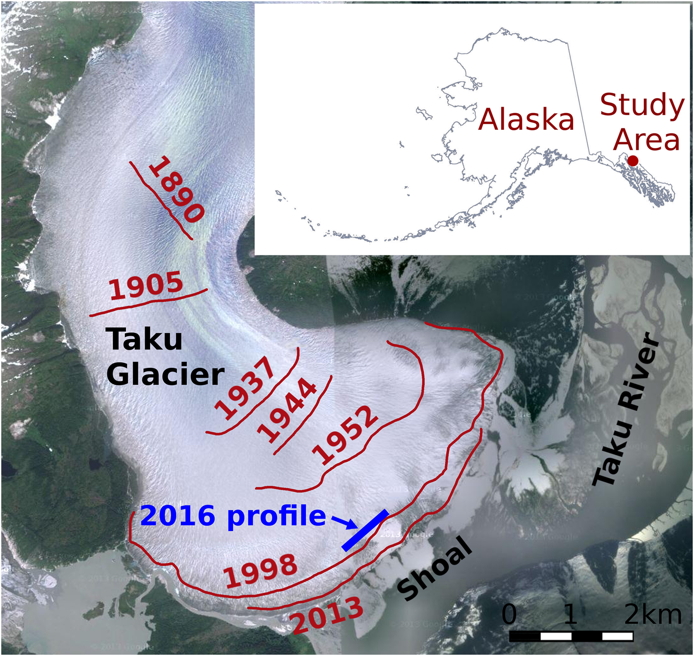
Fig. 2. Taku Glacier terminus, showing the approximate location of the 2016 seismic survey. Historical terminus locations are shown in red (Motyka and others, Reference Motyka, Truffer, Kuriger and Bucki2006). Imagery is from 2010 (Google Earth).
In its advancing phase Taku Glacier is stabilized by a proglacial moraine, which shields the ice from the tides and warm water of Taku Inlet (Kuriger and others, Reference Kuriger, Truffer, Motyka and Bucki2006). During this phase, the glacier advances by excavating subglacial sediments and expelling them in debris flows to form this moraine (Motyka and others, Reference Motyka, Truffer, Kuriger and Bucki2006). As the glacier excavates sediments, its bed becomes overdeepened. Once sediment loss and/or climate change triggers a retreat, the glacier will rapidly lose mass as it calves into deeper and deeper water. In its retracted phase, Taku Glacier leaves behind a fjord (Taku Inlet) that eventually becomes filled in with outwash sediments from the glacier and fluvial sediments from the Taku River (Nolan and others, Reference Nolan, Motkya, Echelmeyer and Trabant1995).
Taku Glacier is currently advancing over fjord sediment deposits (Post and Motyka, Reference Post and Motyka1995; McNeil, Reference McNeil2016) and offers an opportunity to study sediments under a tidewater glacier terminus. Taku Glacier experiences low strain rates compared with other Alaskan tidewater glaciers (Pfeffer and others, Reference Pfeffer, Cohn, Meier and Krimmel2000; O'Neel and others, Reference O'Neel, Echelmeyer and Motyka2003; Truffer and others, Reference Truffer, Motyka, Hekkers, Howat and King2009), resulting in less crevassing which allows us to perform seismic reflection surveys on its surface. We performed such a survey in March 2016 in order to obtain observations of Taku subglacial sediment properties using AVA analysis. The seismic line was located in the ablation area, ~1 km from the terminus and oriented perpendicular to glacier flow (Fig. 2).
Taku Glacier most likely overlies thick sediments in the area of our seismic line. Radar data from Motyka and others (Reference Motyka, Truffer, Kuriger and Bucki2006) show that the glacier bed in the area of our 2016 survey lies at an elevation of ~−90 m at its deepest, 20 m below the fjord bottom mapped in 1890. Bathymetric maps (Post and Motyka, Reference Post and Motyka1995) show that the deposition rate in the area of our seismic line was ~ 0.3 m a−1 from 1890 to 1937. This would extrapolate to a 1750 fjord bottom elevation of ~−110 m.
If we assume this, our seismic line is still >20 m above the 1750 fjord floor, which itself probably was not a bedrock surface. Marine seismic surveys in similar fjords show that the bedrock surface can be deeper than 300 m below sea level (Post and Motyka, Reference Post and Motyka1995). If the same were true of Taku Inlet, the subglacial sediment layer would be at least 220 m thick at the location of our seismic survey.
2.2. Taku glacier sediment samples
Small sediment samples were recovered with a gravity corer in August 2015 from two boreholes at the site of the 2016 seismic survey. They consisted of sandy clays with water contents of 15–24% and 16–26%. Sample densities could not be obtained, so the porosities of these samples are unknown. Upper porosity limits of 34–45% and 35–47% are calculated based on a solid fraction density of 2600 kg m−3, a reasonable density for the local bedrock, which consists of tonalite (Gehrels and Berg, Reference Gehrels and Berg1992).
Our calculated porosity ranges indicate a dilatant till, though uncertainties in water content do not rule out a dewatered till. The sample porosities could fall into the dewatered range if we unintentionally added water during the extraction process and/or overestimated solid fraction density. The sediment could also have experienced dewatering due to the gravity corer method (Talalay, Reference Talalay2013) to the effect that our range underestimates the sample porosity.
2.3. Taku glacier seismic experiment
To perform the seismic survey, we deployed 120 40 Hz geophones spaced at 5 m and buried in a vertical orientation 1 m below the surface. The geophones were installed at the southern end of the seismic line and sources were initiated along the entire 930 m long line. Sources were spaced at 10 m intervals and consisted of 120 g charges of Kinepak installed in boreholes which were backfilled with snow. Boreholes were 5 m deep (the top 1 m was snow with ice below that).
From this survey, we obtained 94 shot gathers. Seismic data processing for viewing the data and picking amplitudes was minimal and consisted of a gain applied to correct for energy loss during spherical spreading. Further data processing was performed to produce a seismic image of the glacier bed. We applied a normal moveout correction using an ice velocity of 3640 m s−1, then stacked common midpoint gathers to produce the seismic image. We derived our ice velocity from the direct wave instead of the glacier bed reflection, as the bed reflection had a lower SNR and exhibited geometrical complexity. The unmigrated image shows that the ice depth increases to the north and varies from ~160 m to 200 m. Based on these depths, the maximum source-receiver angle would be ~70°.
Figure 3 shows the shape of the glacier bed obtained from the stacked unmigrated seismic image, as well as the modeled ray tracing from one shot. This figure illustrates the effects of a rough bed on the propagation of seismic energy. Because the glacier bed is not planar, a sampling of the glacier bed is not uniform and incidence angles do not always increase with offset. Note also that the glacier bed shape in the figure is only an estimation. Our stacked common midpoint gathers may not share the same depth points and arrivals could also originate from outside the vertical plane with the seismic line. As such, it is not straightforward to define the reflection point of either a seismic reflection or its multiple.

Fig. 3. The 2016 survey geometry with ray tracing for one shot. Only rays for every 2nd receiver are shown, for clarity.
The Taku Glacier data suffer from unwanted signal interference. Ground roll contamination strongly affects bed reflections from traces up to 200 m offset from the energy source (Fig. 4).

Fig. 4. An example of a divergence-compensated, but otherwise raw seismic record from the 2016 Taku survey. Amplitudes are multiplied by travel time to correct for spherical spreading. The left lower panel shows a clear bed reflection. The right lower panel shows a signal that could be a bed reflection multiple, though wavelets are oddly-shaped due to groundroll interference.
3. AN AVA FORWARD MODEL
In order to better understand the Taku Glacier seismic data, we first test AVA analysis methods on synthetic datasets. This allows us to gauge the ability of reflectivity methods to estimate subglacial velocity and density in the presence of noise. We are also able to investigate the specific effects of different noise sources and processing techniques.
The forward model uses a specified glacier bed, surface and crevasse geometry, a set of seismic parameters for the bed, an acquisition geometry similar to our field experiment and a realistic source wavelet. We assume that the glacier ice has a uniform seismic velocity, that there is no firn and that the subglacial material is uniform and thicker than 1/4 of the seismic wavelength (~10 m at the center frequency of 100 Hz), so that thin-layer effects do not distort the reflection wavelets (Widess, Reference Widess1973). In reality, dilatant till layers are often thinner (Iverson and others, Reference Iverson, Hanson, Hooke and Jansson1995; Porter and Murray, Reference Porter and Murray2001; Evans and others, Reference Evans, Phillips, Hiemstra and Auton2006; Reinardy and others, Reference Reinardy2011; Booth and others, Reference Booth2012), but a consideration of thin layer effects is beyond the scope of this paper.
We choose some typical values for dilatant till seismic parameters: ρ = 1800 kg m−3, based on a porosity of 50% and a solid fraction density of 2600 kg m−3, α = 1700 m s−1 and β = 200 m s−1, which are all within the range of observed values in Table 1.
We generate synthetic data by assuming that the seismic ray paths can be described by Snell's Law and that the seismic energy can be described by spherical spreading losses, losses due to internal friction, and losses due to reflection(s). We further assume that reflections are from specular interfaces (either crevasses or the bed). We calculate the travel path between a source and a receiver along two possible ray paths: a reflection from the bed and a surface path that interacts with (possibly many) crevasses. Reflection losses are calculated with a Zoeppritz equation Matlab script (Krebes and Margrave, Reference Krebes and Margrave1991; Aki and Richards, Reference Aki and Richards2002). We account for attenuation from internal friction by convolving the source wavelet with a frequency-dependent constant seismic quality factor (Q) impulse response (Kjartansson, Reference Kjartansson1979; Margrave, Reference Margrave1999).
We use a 1 m digital surface model (DSM) of a deglaciated valley as a model input. We choose the Green Lakes Valley in the Colorado Front Range, which Anderson (Reference Anderson2014) used to illustrate a typical lumpy glacier valley. Two lakes cause flat spots to appear in the DSM; we transform these into depressions. For the ice surface we use a parabolic sheet inclined by 2° relative to the DSM, with a glacier outline defined by the intersection of the ice surface with the DSM. The DSM (760 m × 1990 m) was resampled to 10 m resolution to conserve memory and computing power. We add a chevron pattern of crevasses at the glacier edges and flow-perpendicular crevasses at the glacier midpoint. Crevasses are spaced ~15 m apart. We find from satellite images (Google Earth) that valley glaciers tend to have crevasses spaced at ~10 m to 20 m intervals.
We base our choices on forward model parameters (wavelet shapes, relative amplitudes, frequencies and anelastic attenuation values) on the 2016 Taku seismic data (Fig. 4). The following describes how we arrived at these parameter values.
3.1. The source wavelet
We design two source wavelets, one parameterized to resemble the Taku Glacier compressional wave arrivals (Fig. 5) and another to have the appearance of Rayleigh waves from the Taku Glacier dataset. Input parameters include frequency, wave damping and the number of nodes. We use Berlage wavelets (Aldridge, Reference Aldridge1990), though other wavelet types could be substituted.

Fig. 5. The Berlage source wavelet. (a) The plain Berlage wavelet. (b) The wavelet with windowed Gaussian-random noise added; the red dashed line shows the window shape. (c) The same wavelet affected by a seismic quality factor impulse response to simulate anelastic attenuation from travel through 200 m of ice. (d) A direct arrival wavelet from the Taku Glacier dataset, recorded 200 m from the shot.
To simulate real data we add windowed white noise to the source wavelet. The noise window has zero amplitude at the start of the first arrival and ramps parabolically up to a maximum amplitude over the first wavelet half-cycle to remain constant for the next two periods. After that, its amplitude halves every two periods. We then use a highpass filter (above 50 Hz) to improve the similarity between the spectra of our real and synthetic wavelets. The resulting waveform is similar to that observed in Taku data (Fig. 5).
3.2. Seismic quality factor
Seismic quality factor Q is the inverse of internal friction, a material property proportional to the fraction of energy a wave loses per cycle as it travels through a material. We require a value for Q to calculate seismic wave attenuation in ice. Our choice for modeling Q is based roughly on observations of the Taku Glacier dataset.
We calculate the seismic quality factor values from stacked common offset gathers of the direct wave. Q is calculated independently for every offset, using the spectral ratio method, in which the frequency spectra of near and far offset direct arrivals are compared (Gusmeroli and others, Reference Gusmeroli2010).
We find that the seismic quality factor varies with shot offset, first increasing and then leveling off. This reflects the fact that direct waves traveling a longer distance sample deeper glacier ice with higher Q-values. Seismic quality factor decreases with degree of material fracture unless the material is fully saturated with water. Thus, we can expect a glacier surface to have low seismic quality factor values, with Q increasing with depth (Gusmeroli and others, Reference Gusmeroli2010; Babcock and Bradford, Reference Babcock and Bradford2014) as voids in the ice become smaller and more water-saturated.
In order to find the seismic quality factor of the deeper ice using the direct wave data, we create a forward model to calculate the average seismic quality factor, Q a, in the Fresnel volume. We assume that the ice thickness is divided into a lower layer where seismic quality factor is constant (Q i) and an upper layer of thickness c = 30 m (equal to the maximum vertical extent of crevassing) where Q z (depth-dependent seismic quality factor) increases linearly from a surface value (Q s) to Q i (1). This is equivalent to a power law decrease in internal friction.
 $$Q_{\rm z} = \left\{ {\matrix{ {Q_{\rm s} + \left( {\displaystyle{{Q_{\rm i} - Q_{\rm s}} \over c}} \right)z} & {{\rm }0 \le z < c} \cr {Q_{\rm i}} & {{\rm }z \ge c} \cr } } \right.$$
Q is found from the average internal friction of the Fresnel zone, which is estimated by numerically integrating  $Q_{ {\rm z}}^{-1}$ over the elliptical Fresnel zone of the surface wave and dividing by total Fresnel zone volume. A model with Q s = 30 and Q i = 230 provides a reasonable fit to the observed Q-values.
The Q-value of the groundroll (Q r) is also calculated following the spectral ratio method. We use a constant seismic quality factor when we calculate Rayleigh wave attenuation (Q r = 12).
3.3. Reflection raytracing
We construct bed reflections using a two-layer raytracing algorithm with a 3D layer interface. Five thousand rays are emanated from each shot location (from angle ranges −90° to +90°) and traced to the bed of the glacier and then to their emergent position on the glacier surface. The density of ray coverage is usually sufficient to provide each receiver position with at least one emergent ray, to within 10 m tolerance.
If the search returns multiple rays for a given geophone, it bins the rays by bed incident location and averages the ray arrival times so that only one arrival per bin is recorded. This model assumes that a lack of rays reaching a geophone is due to an insufficient density of modeled rays, so if no rays are returned to a geophone within the search radius, the nearest surface-incident ray is chosen. To conserve computing speed, we chose not to increase the number of modeled rays.
We then produce the reflection wavelet scaled by bed reflectivity, geometric spreading and anelastic attenuation. Since bed reflected rays interact with all layers of ice, we calculate a bulk average Q-value using (1).
A bed reflection multiple is modeled by continuing to trace the surface-incident ray to the glacier bed again and back to the surface. We record the longer travel time and transform the multiple wavelets based on Q and spherical spreading accordingly. We also scale the wavelet by the product of the reflectivities of its two reflections with the bed and its reflection with the surface. We approximate the reflectivity of the ice/air interface as −1; due to acquisition geometries, recorded multiples will have ice-air reflection incidence angles  ${\vskip 10pt\lt \atop \vskip -12pt\approx}\! 40^{\circ }$ (see Fig. 1).
3.4. Reflections from surface features
The model includes backscattered signals from crevasses when it calculates direct wave and Rayleigh wave arrivals. Backscattered direct waves and surface waves are clearly visible in the Taku seismic data (see Fig. 4).
We choose a general ‘reflectivity’ c r (proportion of backscattered vs transmitted energy, converted to amplitude) of crevasses in order to produce a noise pattern, loosely based on that observed in the Taku Glacier data, that we deem realistic and desire to test. We choose a c r value of 0.3, and hold it constant for every crevasse reflection in the model regardless of incident angle or crevasse size. Note that in reality, c r depends on the ray incident angle with the crevasse and the size of the crevasse relative to the wave Fresnel zone (Benjumea and Teixidó, Reference Benjumea and Teixidó2001); we ignore these considerations because our c r is just a crude approximation of highly variable values.
We determine Rayleigh and direct wave arrival times using a 2-D raytracing model, treating crevasses as planar reflectors. This is an approximation that allows us to produce different levels of surface wave noise and different arrival patterns of surface wave noise.
Ray amplitudes decrease as they are transmitted past or reflected off of crevasses. The rays that propagate past the crevasse have amplitudes equal to  $\sqrt {a_{ {\rm i}}^2 - (c_{ {\rm r}} a_{ {\rm i}})^2}$, where a i is the amplitude of the incident ray. The amplitude of the reflected ray is c ra i.
Rayleigh waves and direct compressional waves also reflect off of glacier sidewalls. We use a 2-D adaptation of the 3-D raytracing algorithm to produce sidewall reflections. Rayleigh wave reflectivity is set to c r for simplicity, while direct wave reflectivity is determined via the Zoeppritz equations and the assumption that the sidewall material is identical to the basal material.
Arrivals from sidewall and surface reflections are sorted in the same way as the bed arrivals. We add scaled Berlage wavelets according to modeled arrivals times and correct the wavelets for spherical spreading and attenuation due to Q a of the wave Fresnel zone.
3.5. Seismic record assembly
Bed reflections, sidewall reflections, primary waves with crevasses and Rayleigh waves with crevasses are calculated separately. All component simulations are sampled at the same temporal sampling interval, therefore no further interpolation is required when assembling them into the full synthetic record. They are simply added together. Very low amplitude nearfield white noise is added to this record to add further realism to the model. Finally, we simulate variability in shot-geophone coupling by multiplying each trace by a factor chosen at random between 0.6 and 1.0. The coupling range is arbitrary and loosely based on observations from the Taku Glacier data.
4. AVA ANALYSIS
We perform AVA analysis on the synthetic seismograms using the procedures discussed below. We then discuss our ability to retrieve the till properties prescribed in the forward model.
4.1. Incidence angle and depth
A normal moveout correction is applied to the model results, using an ice velocity calculated from the first breaks of the stacked direct wave. Common-midpoint gathers are stacked to produce a seismic image. We assume that the first breaks of the stacked section represent the bed cross section directly under the seismic line. Incidence angles and locations for each reflected wave are derived from a forward model of raypaths using this bed shape.
4.2. Shot-geophone coupling
We determine the RMS amplitudes of the direct arrival wavelets. Amplitudes are corrected for spherical spreading by multiplying by x −1, where x is the direct wave raypath length. Direct waves are also multiplied by e ax to correct for anelastic attenuation. a is found from
 $$a = \displaystyle{{\pi f} \over {\alpha _{{\rm ice}}Q_{\rm a}}},$$
where α ice is the compressional wave velocity of the ice and f is the dominant frequency of the wavelet. We determine Q s and Q i from the synthetic data using the same process we employed with the 2016 Taku data and find Q a for each direct wave using (1) and integrating  $Q_{ {\rm z}}^{-1}$ over the Fresnel zone volume.
Attenuation-corrected direct wave amplitudes are normalized to their average and these normalization factors are assumed to correct for shot-geophone coupling variability. We multiply the amplitudes of each raw trace by its corresponding entry in the normalization vector.
4.3. The reflectivity curve
We pick the amplitudes of the bed reflection wavelets and near-offset bed reflection multiple wavelets. With these amplitudes and raylengths and with source amplitude A 0, we can calculate bed reflectivity R using:
 $$R = \displaystyle{{A_1} \over {A_0{\mkern 1mu} \gamma }}{\mkern 1mu} e^{ax},$$
where A 1 is the bed reflection amplitude, x is the raypath length and a is calculated from (2) using the average Q-value of the entire ice thickness and the center frequency of the bed reflection. The factor γ is a geometrical correction term,
 $$\gamma = \displaystyle{1 \over x}\cos \left( \theta \right)$$
where θ is the angle at which the seismic wave reaches the receiver.
We calculate A 0 using
 $$A_0 = \displaystyle{{A_1^2 } \over {A_2}}{\mkern 1mu} \displaystyle{{\gamma _2} \over {\gamma _1^2 }}{\mkern 1mu} {\rm e}^{2a_1x_1 - a_2x_2}$$
from Peters (Reference Peters2009), where A 2 is the amplitude of the bed reflection multiple. Equation (5) requires that A 1 and A 2 have similar incidence angles (we require incidence angles to be within 5° of each other). We calculate γ, a and x separately for the reflection and multiple.
This method has the potential to produce an error due to geophone coupling variability and the fact that A 1 and A 2 sample different parts of the seismic interface, unless A 1 and A 2 are zero-offset and co-trace. However, due to shot proximity and groundroll noise, we are unable to find useable zero offset, co-trace A 1 and A 2 arrival pairs in real data and all synthetic runs except the Flat run.
The reflectivity of every wavelet is calculated using (3). These reflectivities yield the AVA curve when plotted against the incidence angle. We invert for ρ, α and β using a grid search to find the best Zoeppritz curve fit in the least-squares sense (Booth and others, Reference Booth2012). Grid search spacing is Δα = 20 m s−1, Δβ = 20 m s−1 and Δρ = 20 kg m−3.
The grid search is restricted to parameter combinations that are physically plausible. α, β and ρ combinations must lay within the range of a dilatant till, a dewatered till, or a consolidated till (see Table 1 for acceptable ranges).
We also test the use of a frequency bandpass filter as well as an FK filter. The bandpass filter has a lower cutoff of 60 Hz, a plateau between 120 Hz and 300 Hz, and a higher cutoff at 600 Hz. Such a filter has worked well to reduce groundroll noise in the Taku 2016 dataset, although not to the point where seismic reflection energy can be recovered at all offsets.
The FK filter is designed to remove signals with velocities less than the compressional wave velocity in ice and also includes a frequency bandpass filter with a lower cutoff of 100 Hz, a plateau between 140 Hz and 260 Hz, and an upper cutoff of 300 Hz. This is more successful than a simple bandpass filter at revealing a greater angle range of the bed reflection signal, but has the disadvantage of affecting reflection wavelet amplitudes to a greater extent.
4.4. Inverting for the source amplitude
We attempt performing AVA without the bed reflection multiple by following the methods of Dow and others (Reference Dow2013). For every combination of α, β and ρ, we compare the modeled Zoeppritz curve with simulated reflectivity curves calculated from the bed reflection amplitudes (binned by incidence angle) and a range of possible A 2 values. The tested range of A 2 values are equally spaced from zero to half of a reference A 1 value. This reference amplitude is equal to the normal-incidence reflection amplitude, or if that is not available, the maximum reflection amplitude. We use the range of A 2 values to calculate corresponding A 0 values using the reference reflection amplitude and (5). Next, we calculate simulated reflectivity curves from each A 0 value.
Simulated AVA curves are rejected if normal incidence reflectivity exceeds 0.6 (the maximum for any type of ice/bed interface), or if the absolute value of reflectivity for any angle exceeds 1. To allow for some data error, we add a buffer of 0.1 to both of these values. We calculate simulated curve misfits (by summing squared residuals divided by the number of datapoints, then taking the square root) and assign the smallest misfit to the grid cell for the tested α, β and ρ combination.
4.5. Crossing angle analysis
Anandakrishnan (Reference Anandakrishnan2003) estimated seismic parameters using reflectivity crossing angle and we test his methods here. A grid search finds α, β and ρ based on the angle at which the phase reversal occurs. In source amplitude inversion, incorrect calculation of attenuation alters the curve shape and changes the results. Crossing angle analysis avoids this problem and furthermore allows us to skip Q calculation and coupling correction.
In the crossing angle inversion process, we define the misfit as the gap between the observed and calculated crossing angles. We also define the maximum acceptable misfit as either the width of an angle bin or, if angle bins adjacent to the crossing are empty, half the width of the gap plus the width of an angle bin.
4.6. Acceptable misfit
In order to characterize an acceptable range of till parameter combinations (α, β, and ρ) in AVA analysis (crossing angle analysis excluded), we calculate an envelope of acceptable Zoeppritz curve fits. We do not perform a rigorous data error analysis here, as the nature of coupling corrections and reflectivity calculations in AVA results in errors that are systematic and non-Gaussian. Instead, we want to define an error range that approximates how far up or down we can shift the best-fit AVA curve before it no longer passes between datapoints; the ‘highest’ and ‘lowest’ it can range defines the envelope.
To fall within the envelope, Zoeppritz curves must satisfy a maximum acceptable error value E max. E max is determined from the best fit Zoeppritz curve and the maximum data residual as follows.
The best-fit curve error (our minimum error E min) is equal to the sum of squares of the differences between the observed reflectivities R d and the best-fit curve R m:
 $$E_{{\rm min}}^2 = \sum_{i=1}^{n}\left(R_{{\rm d}}(i) - R_{{\rm m}}(i)\right)^2.$$
Here, n is the number of datapoints.
We now find the maximum residual, h, in the dataset,
 $$h = \max{\left(\vert R_{{\rm d}}(i) - R_{{\rm m}}(i) \vert \right)},$$
then we shift the best-fit curve up by h (approximating the top of our envelope) and re-calculate the error (6). We then define a maximum acceptable error as
 $$E_{{\rm max}}^2 = \sum_{i=1}^{n}\left(R_{{\rm d}}(i) - R_{{\rm m}}(i)+h\right)^2.$$
Multiplying the terms in (8), we obtain
 $$E_{{\rm max}}^2 = \sum_{i=1}^{n} (R_{{\rm d}}(i) - R_{{\rm m}}(i))^2 + \sum_{i=1}^{n}(R_{{\rm d}}(i) - R_{{\rm m}}(i))h + nh^2.$$
Assuming that the middle term is negligible because
 $$\sum_{i=1}^{n}R_{{\rm d}} \approx \sum_{i=1}^{n}R_{{\rm m}},$$
Equation 9 reduces to
 $$E_{{\rm max}}^2 = \sum_{i=1}^{n} (R_{{\rm d}}(i) - R_{{\rm m}}(i))^2 + nh^2 = E_{{\rm min}}^2 + nh^2.$$
We convert this to a maximum misfit value by dividing  $E_{ {\rm max}}^2$ by the number of datapoints and taking the square root:
 $$\sigma _{{\rm max}} = \sqrt {\displaystyle{{E_{{\rm max}}^2 } \over n}} ,$$
where σ max is the maximum misfit.
We now examine the results from our grid search over α, β and ρ and designate all combinations with misfits smaller than σ max as acceptable.
4.7. Acoustic impedance
The α, β and ρ grid search results may also be expressed as an acoustic impedance (Z) vs β parameter space, where Z = αρ. For easier viewing of our results, we translate the α, β and ρ combination misfits into a Z vs β misfit plot. A problem arises at this step as numerous combinations of α and ρ produce the same Z, yet result in different AVA curves (and curve misfits), even as β is held constant. We address this problem by using the lowest misfit combination of α and ρ for each β, Z pair.
Tested Z values from our grid search are not uniformly spaced, so we perform a resampling of the Z vs β misfit function by binning misfits by Z and taking the mean misfit value, then applying a 2-D Gaussian filter to the misfit plot. Note that this causes the Z vs β plots (Fig. 6) to show best-fit β values and acceptable ranges that differ slightly from the α, β and ρ grid search results (Fig. 7 and 8). We use only α, β and ρ grid search results when reporting best-fit values and acceptable ranges for β.

Fig. 6. Parameter ranges returned by AVA analysis of model runs and Taku Glacier data, showing best fit values (dots) and acceptable ranges (whiskers). Subscripts following chart labels refer to the following AVA methods: no subscript, source amplitude inversion; A 0, source amplitude calculation; x, crossing angle analysis; fk, source amplitude inversion with an FK filter applied; x−fk, crossing angle analysis with an FK filter; bandpass, source amplitude inversion with a bandpass filter.

Fig. 7. AVA results from synthetic seismic records. Tables (left) show best-fit parameter combinations and acceptable ranges, which result in the red dashed curves and gray-dashed curve envelopes in the reflectivity vs incidence angle plots (center); data reflectivities or crossing angles appear as blue dots, and the green curve is the model input. To the right are acoustic impedance (Z) vs β misfit plots; boxes labeled A, B and C encompass the dilatant till, dewatered till and consolidated till ranges, respectively. White lines mark the range of acceptable Z vs β combinations and white crosses mark the best-fit Z, β pair.
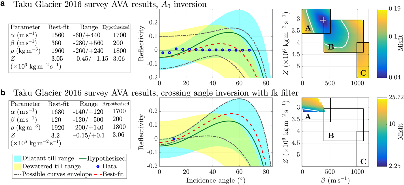
Fig. 8. AVA curve fits to reflectivities calculated from the Taku Glacier seismic record.
5. RESULTS
We perform three model runs which are distinguished from one another by input geometry (Table 2). AVA analysis is performed on these synthetic datasets (Flat, GL-long and GL-trans), as well as the real data from Taku Glacier.
Table 2. Model runs.

5.1. Deep, flat glacier run (‘Flat’)
In the Flat model, the bed reflection and the multiple are easily identified and it is possible to complete a full AVA analysis. This returns seismic parameters that are close to the input parameters and lie within dilatant till ranges (Fig. 7 Subplot A). Traditional AVA produces a misfit function with a well-defined minimum, resulting in a narrow solution range. A 0 inversion also results in a well-defined, but somewhat broader minimum which correctly establishes the till as dilatant (Fig. 7 Subplot B).
When we invert for the crossing angle only, we also obtain acceptable parameter values that fall completely within the dilatant till range. Misfit plots do not center on a local minimum, but rather a trough. The relationship between acoustic impedance Z and β is well-constrained, but there is little variation in misfit value along that line.
5.2. Longitudinal Green Lakes Valley run (‘GL-long’)
This model run uses the Green Lakes Valley geometry and a seismic line that is parallel to the glacier axis and perpendicular to crevasses (Fig. 9). The survey samples a relatively flat part of the glacier bed, keeping the raypaths simple. In the output seismic gathers (see Fig. 10 for an example), the multiple is obscured and so is part of the bed reflection. A crossing angle becomes visible when we apply an FK filter to the data; crossing angle analysis reveals the tills as dilatant (Fig. 7 Subplot D). Without an FK filter, no crossing angle is visible and source amplitude inversion yields parameters that extend into the dewatered till range (Fig. 6 and Fig. 7 Subplot C.

Fig. 9. GL-long (magenta) and GL-trans (red) survey setup. Geophones are marked as dots. Examples of raypaths (red and magenta lines) are shown emanating from shots (yellow asterisks) and reflecting off of the Green Lakes Valley surface and returning to geophones (red and magenta dots). Cyan lines represent modeled crevasses.

Fig. 10. An example of divergence-compensated, but otherwise raw seismic records from the GL-long and the GL-trans synthetic data. Amplitudes are multiplied by travel time to correct for spherical spreading. Insets show close-ups of the bed reflection and the expected location of the normal-incidence bed reflection multiple. In both seismic gathers, the ground roll signal completely obscures the multiple.
5.3. Transverse Green Lakes Valley run (‘GL-trans’)
A geometry with a transverse seismic line (parallel to crevasses, Fig. 9) produces a seismogram that looks very different from its longitudinal counterpart (Fig. 10). In GL-trans, the bed reflection is affected by overlaying hyperbolic signals where the direct wave has reflected off of crevasses. These signals resemble the bed reflection.
No multiple is visible, so we are limited to crossing angle analysis or A 0 inversion to perform AVA on this dataset. Applying an FK filter does not improve bed reflection SNR enough to see a polarity reversal, so A 0 inversion is our only course of action. Unfortunately, after A 0 inversion, possible parameter combinations exist in the dewatered till range (Fig. 6 and Fig. 7 Subplot E). Thus AVA fails to uniquely identify the till as dewatered or dilatant.
5.4. Taku Glacier 2016 survey data analysis
A signal that resembles a bed reflection multiple appears in the Taku Glacier dataset but applying AVA using this ‘multiple’ results in reflectivities greater than one. Thus we believe that this signal is a primary reflection from a large parallel crevasse or from a different part of the glacier bed and a multiple reflection is not visible.
Instead of traditional AVA, we perform source amplitude inversion and crossing angle analysis. The source amplitude inversion method is not precise enough to reveal till types in this case (Fig. 8 Subplot A), but crossing angle analysis produces acceptable parameter combinations that fall completely within the dilatant till range (Fig. 6 and Fig. 8 Subplot B).
6. DISCUSSION
6.1. Influence of noise
The largest impact on data quality was increased surface wave noise from crevasse backscattering. The amount of noise varied between GL-long and GL-trans due to differences in crevasse orientation producing different patterns of noise arrival times. GL-long produces a seismic record that allows AVA analysis, whereas GL-trans data fails AVA analysis. In GL-long, destructive interference resulting from modeled crevasse spacing caused decreased noise (Fig. 10). Crevasses in GL-trans are parallel to the seismic line and arrivals from them constructively interfere. Furthermore, crevasses parallel to the seismic line produce arrival times in hyperbolic patterns which resemble and could occur within a wavelength of the bed reflection, making picking difficult.
6.2. Ice thickness and AVA
Our modeling approach has allowed us to analyze geometry requirements for a successful AVA survey, assuming the seismic source and ice qualities of our Taku Glacier survey. With this model, we can predict the quality of the seismic survey before entering the field.
We observe in our model results that, at some critical ice thickness, the direct wave and/or its reflections from nearby crevasses dominates the bed reflection signal even before Rayleigh waves arrive. This critical ice thickness is dependent on compressional wavelength, the amount and duration of noise that trails the wavelet, the character of crevasse dispersion noise and the reflectivity of the glacier bed. In the best-case scenario (no crevasses, no noise trailing the direct wavelets) and with our model parameters, ice must be >46 m thick to avoid interference with the bed reflection at 60° offset, or >26 m thick for bed reflections up to 40° offset. These thicknesses will vary from survey to survey according to the shape of the direct wavelet, which depends on the frequency spectrum and impulse duration of the seismic energy source.
At this minimum thickness, modeled random noise trailing the direct wave still overlaps with the reflection signal, obscuring the shape of the bed reflection wavelet at angles with very low reflectivities. To avoid bed reflection contamination at 60° offset with the highest-amplitude part of our modeled noise tail, the ice thickness would need to be >115 m. This number varies between seismic surveys depending on the length and amplitude of noise associated with the direct arrival.
Bed reflections appear clearly in GL-trans despite the fact that ice thickness is only 70 m, because crevasse signals fortunately interfere destructively. Without this destructive interference, the ice would have to be much thicker for the bed reflection to arrive after crevasse noise is sufficiently attenuated. Such crevasse signals seen in the Taku Glacier data last up to 0.026 sec after the direct wave arrival, which results in a minimum glacier thickness up to ~180 m for a 60° offset. Within a 40° reflection angle, this minimum thickness decreases to 100 m. In order to distinguish a reflection at incidence angles past the groundroll signal (>25°) the glacier would need to be 76 m thick. This assumes the worst case crevasse spacing for the direct compressional signal wavelength (even and continuous at increments of 22-28 m). With fewer crevasses, thinner ice is acceptable.
In a scenario with many reflectors parallel to the seismic line, surpassing the minimum thickness does not guarantee a usable bed reflection because unwanted reflection hyperbolas could overlay the glacier bed signal at any depth.
6.3. Quality factor inversions
Underestimating or overestimating Q had little impact on AVA uncertainty in our experimental runs. Its effect on reflectivity calculations was superceded by other sources of error. However, Q errors could become more important in other survey scenarios, such as when Q is exceptionally low or if AVA can only be accomplished via source amplitude inversion, thus requiring an accurate reflectivity trend. Q has the potential to introduce false trends if a coupling correction is applied to the data. The effect of overestimating attenuation, for example, is that the correction vector amplifies bed returns as receiver offset increases.
To examine the importance of Q uncertainties, we re-ran AVA analysis using the model inputs for Q i and Q s (Fig. 11). The bars labeled ‘Normal’ correspond to the source amplitude inversion procedure using unfiltered data, incidence angles calculated by raytracing, and seismic quality factors calculated from the seismic line. ‘Known Q’ bars correspond to AVA results using the Q values from the forward model (Q i = 230 and Q s = 30). Bar charts show metrics for accuracy and precision. Accuracy is quantified by the percentage of acceptable parameter combinations that lie outside the range of a dilatant till (first row) and the misfit between the best-fit curve and the input curve over tested incidence angles (third row). The second row quantifies precision and shows the size of the acceptable parameter combination range as a percentage of all tested parameter combinations. Smaller values for all three metrics correspond to higher accuracy or precision.
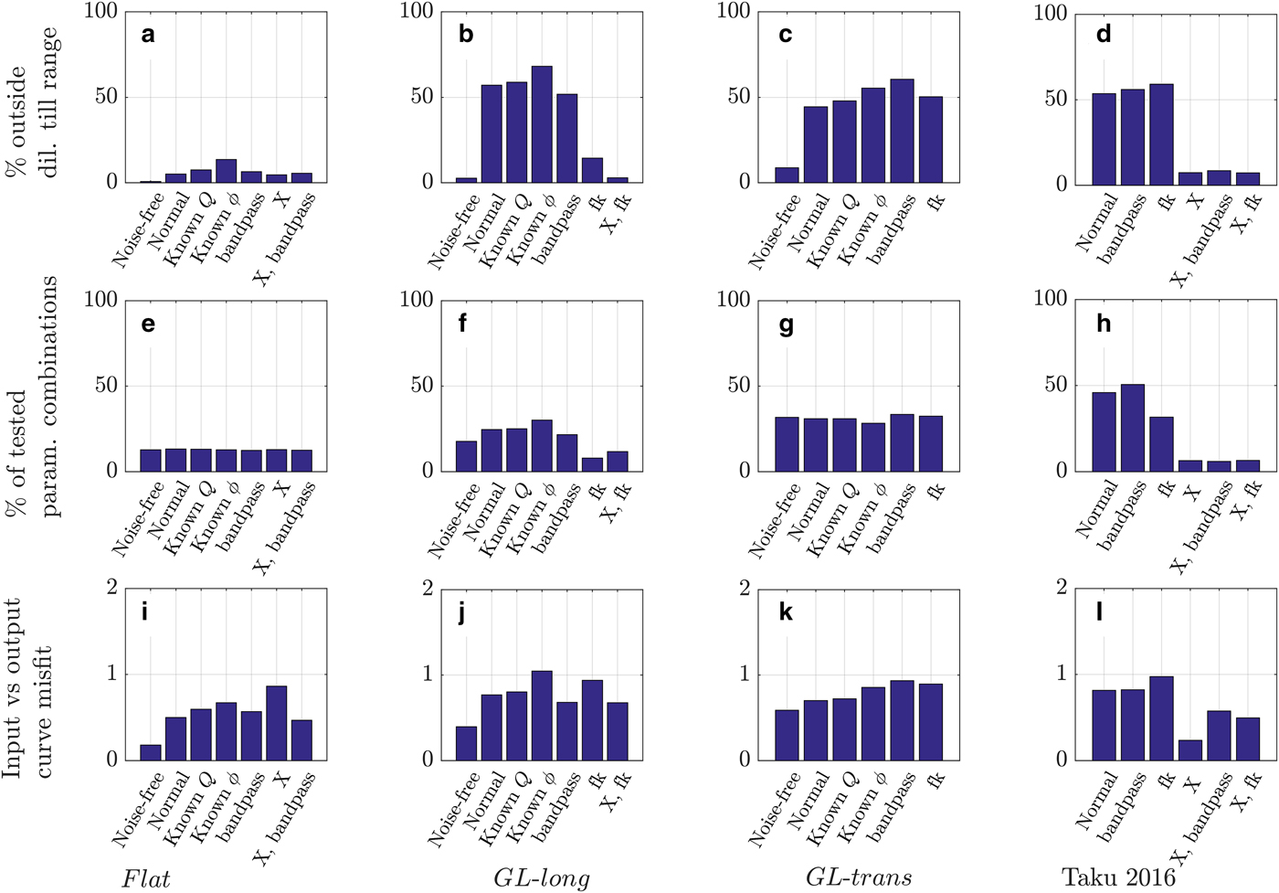
Fig. 11. Metrics for accuracy and precision for synthetic model runs. Lower values indicate higher success. Columns show different model runs. Top row: percent of parameter combinations that lie outside of the dilatant till range. Middle row: percent of allowable parameter combinations out of all tested parameter combinations. Bottom row: the misfit between the best fit and the input AVA curves. Results are from source amplitude inversion unless indicated otherwise. Bars in the same plot represent different improvements or modifications to the AVA analysis, either by FK or bandpass filtering the data, substituting in the original Q or ϕ values, or performing crossing angle analysis (abbreviated as ‘X’) with or without a bandpass or FK filter.
Using correct Q values causes very little change in AVA results for all models using source amplitude inversion. Results were not very sensitive to Q-value calculations, even though calculated Q-values for GL-long and GL-trans differed significantly from the prescribed values (Table 3).
Table 3. Calculated seismic quality factors from model runs.

6.4. Reconstructions of incidence angles: the effects of incorrect ϕ
The GL-trans run is the most geometrically complex and produces the least-reliable raytracing results. Depth points and incidence angles calculated using the brute stack are within a median distance of 2° and 16 m (26% of the glacier thickness) of the real forward model depth point and incidence angle values, respectively. The 75th percentile incidence angle difference is smaller than our 5° angle bins, so it seems unlikely that incidence angle miscalculations could affect our results. Fig. 11 shows that GL-trans AVA accuracy (measured as misfit between input and best-fit curves) and precision (measured as mean R range or percent of parameter combinations outside of the dilatant till range) does not improve with incidence angle accuracy.
The GL-trans profile overlays ice that is only 70 m deep and yet our errors in calculated depth points range up to a few tens of meters. This would be problematic if we desired to bin bed reflections by depth point to look for spatial variability in till qualities. For GL-trans, we would need to choose a bin size of ~30% of the ice thickness or greater to reflect this uncertainty.
6.5. Effects of survey ϕ range
In this experiment, we found that crossing angle analysis is the most reliable tool for confirming a subglacial dilatant till. Crossing angle analysis is limited by the incidence angle range of observable bed reflection polarities, however. Dilatant tills have polarity reversals at low incidence angles ( $\phi {\vskip 10pt\lt \atop \vskip -12pt\approx}30^{\circ }$; ϕ = 20° for our input parameters), where the bed reflection can be obscured by groundroll waves. However, a wide range of glacier bed materials, including dilatant tills, also exhibit polarity reversals at greater ϕ values (70° for our modeled dilatant till). Extending a seismic survey line past this incidence angle could increase the ability to constrain glacier bed type. A single observation of positive polarity past ϕ > 70° can rule out dewatered tills and consolidated tills as the subglacial layer, for example (Fig. 1), though it cannot distinguish between dilatant tills and bedrock. Placing a single receiver at a very far offset ( ${\vskip 10pt\gt \atop \vskip -12pt\approx}$6 times the ice thickness from the farthest seismic source for ϕ > 70°) could be an inexpensive and useful addition to an AVA survey with a short line.
6.6. Effects of bandpass and FK filtering
FK filtering was the only processing method that allowed us to recover input till type in the GL-long model run, as its suppression of surface wave noise allowed us to locate a polarity reversal in the bed reflection for crossing angle analysis. This polarity reversal clearly established the till as dilatant. We did not experience the same success when applying an FK filter to GL-trans, as GL-trans had more backscattered noise from compressional waves, which could not be filtered out without also removing the bed reflection.
Bandpass filtering, though less effective at removing groundroll noise than FK filtering, carries some advantages over FK filtering. An FK filter requires a close geophone spacing; the 5 m spacing of the Taku survey and the 10 m spacing of the Greenlakes surveys were sufficiently small, but the 60 m Flat survey spacing ruled out an FK filter as an option. Bandpass filtering, though unnecessary for the Flat data and leading to no advantage in accuracy or precision, could still be applied. Bandpass filtering was also applied to the GL-trans and GL-long model runs, though did not improve source amplitude inversion results and did not reveal near-offset returns. In GL-long, an FK filter did improve accuracy in the source amplitude inversion method and allowed for a crossing angle analysis, as mentioned previously. No processing methods were able to improve results in the case of GL-trans–unless noise was removed completely from the synthetic run (see the ‘Noise-free’ bar).
We found that filtering was not required for a successful crossing angle analysis in the case of Taku Glacier; though groundroll covered up many returns at near offsets, the shape of the glacier bed (having a dip in the middle of the line) ensured that a sufficient number of incidence angles were sampled to perform a crossing angle analysis–though one of the incidence angle bins closest to the reversal only included two datapoints. Bandpass and especially FK filtering were better at populating angle bins with bed polarity observations.
6.7. Shot-geophone coupling corrections
We found that our AVA results were not very sensitive to the application of shot-geophone coupling corrections. Such corrections would be more useful in a case where shot strength and geophone coupling were more variable. It is possible that errors in attenuation calculations could cause the coupling correction to introduce false amplitude trends, so the researcher should check the coupling correction vector for unrealistic offset-dependent trends.
7. CONCLUSIONS
This study affirms the notion that deeper and less-crevassed glaciers with simple bed geometries are the best candidates for AVA studies (Fig. 12). At the other end of the spectrum, very thin (<100 m) heavily-crevassed glaciers cannot yield data suitable for AVA analysis.

Fig. 12. Conceptualization of AVA survey quality based on ice thickness and degree of crevasse noise. Each blue dot marks a reported reflectivity survey. Red dots are from modeled surveys. Degree of crevasse noise is from remarks made by the author, or we estimate it from photographs or satellite imagery of the studied glacier.
Glaciers in the middle of the spectrum–without workable bed reflection multiples, but with bed reflections that are not overwhelmed by crevasse noise–can be successful AVA candidates. A near-offset crossing angle confirms a dilatant till, as long as crossing angle can be recovered after FK or bandpass filtering. Source amplitude inversion is a reasonable method if source amplitude is uncertain and it is not possible to identify glacier bed type using crossing angle analysis. However, for source amplitude inversion to work, bed reflection SNR must be high enough to reveal an amplitude trend. In the case of a high-quality bed reflection but an uncertain A 0, source amplitude inversion may be as accurate as AVA. It avoids the possibility of unquantified errors in the source amplitude calculation skewing results.
This forward model serves as a planning tool for seismic surveys on thin, crevassed, geometrically-complex glaciers. Crevasse locations can be obtained from satellite imagery of the glacier surface. The glacier bed can be constrained using existing radar data or, barring that, an estimated glacier bed that combines a typical glacier width/depth ratio with the maximum amount of basal topography that can be reasonably expected. If AVA is successful from the simulated data despite the high amplitude of basal topography, then it should be successful with the study glacier. The model could be run with the hypothesized till parameters and perhaps repeated with the local bedrock to ensure the two can be distinguishable from each other. Model results can also indicate the best use of resources in the seismic survey. If the bed reflection is obscured at near offsets due to crevasse noise, shots should be located farther away from the geophone line. However, this will make it impossible to use a direct calculation of the source amplitude.
Our synthetic survey results show that geometry uncertainties do not significantly impact AVA results. Because of this, we are confident that the Taku Glacier AVA results are not misleading, even with only an estimate of the glacier bed shape. Our brute stack did not show a basal topography that was as rough as the GL-trans topography, so our ϕ calculation errors could not have exceeded the GL-trans errors. It is probable that the Taku Glacier incidence angle calculation errors were smaller than the size of our angle bins, so the topography beneath the Taku Glacier seismic line could not have caused a till type misidentification.
Crossing angle analysis shows that Taku Glacier sediments are within the range we have defined as dilatant and as a consequence, are deformable. A deformable till under Taku Glacier has consequences for its terminus evolution. Till deformation allows faster evacuation of sediments from beneath Taku Glacier, as deforming till creeps towards subglacial channels, where it can be eroded fluvially–an important mechanism for sediment evacuation (Motyka and others, Reference Motyka, Truffer, Kuriger and Bucki2006) and tidewater glacier dynamics (Brinkerhoff and others, Reference Brinkerhoff, Truffer and Aschwanden2017).
CONTRIBUTION STATEMENT
JZ performed most of the writing of this paper, most of the model development, led the seismic survey portion of the fieldwork performed on Taku Glacier in 2016, and performed all analysis of the 2016 seismic dataset with the advice and supervision of MT. MT, AG, JA and CL conceived of the study and participated in the field work. AB proposed and produced a preliminary version of the forward model and advised on AVA processing strategies. AG helped with seismic data processing. All authors contributed to the writing of the manuscript.
ACKNOWLEDGEMENTS
The Taku 2016 survey was made possible by input and assistance from Thomas Hart (blaster), Aurora Roth, and Andy Aschwanden. IRIS PASSCAL provided seismic recording equipment for the Taku 2016 seismic survey. Thanks to Peter Burkett, Sridhar Anandakrishnan and Kiya Riverman for instrument support, and to Bernard Coakley, Bernard Hallet, Esther Babcock and some anonymous reviewers for their input and advice. Also thanks to the Consortium for Research in Elastic Wave Exploration Seismology (CREWES) for providing Matlab scripts that facilitated the seismic forward modeling. This project is funded by National Science Foundation grant number 130 4899 and supported in part by a University of Alaska Fairbanks Center for Global Change Student Research Grant with funds from the Cooperative Institute for Alaska Research.


 Open access