


1 Introduction
The method for analyzing the asymptotic cost of a (functional) program f(x) that is typically taught to introductory undergraduate students is to extract a recurrence  $T_f(n)$ that describes an upper bound on the cost of f(x) in terms of the size of x and then establish a nonrecursive upper bound on $T_f(n)$ (we will focus on upper bounds, but much of what we say holds mutatis mutandis for lower bounds, and hence tight bounds). The goal of this work is to put the process of this informal approach to cost analysis on firm mathematical footing. Of course, various formalizations of cost analysis have been discussed for almost as long as there has been a distinct subfield of Programming Languages. Most of the recent work in this area is focused on developing formal techniques for cost analysis that enable the (possibly automated) analysis of as large a swath of programs as possible. In doing so, the type systems and the logics used grow ever more complex. There is work that incorporates size and cost into type information, for example, by employing refinement types or type-and-effect systems. There is work that formalizes reasoning about cost in program logics such as separation logic with time credits. But as witnessed by most undergraduate texts on algorithm analysis, complex type systems and separation logic are not commonly taught. Instead, a function of some form (a recurrence) that computes the cost in terms of the size of the argument is extracted from the source code. This is the case for “simple” compositional worst-case analyses but also more more complex techniques. For example, the banker’s and physicist’s methods of amortized analysis likewise proceed by extracting a function to describe cost; the notion of cost itself, and the extraction of a suitably precise cost function, is more complex, but broadly speaking the structure of the analysis is the same. That is the space we are investigating here: how do we justify that informal process?Footnote 1
The justification might not itself play a role in applying the technique informally, any more than we require introductory students to understand the theory behind a type inference algorithm in order to informally understand why their programs typecheck. But certainly that theory should be settled. Our approach is through denotational semantics, which, in addition to justifying the informal process, also helps to explicate a few questions, such as why length is an appropriate measure of size for cost recurrences for polymorphic list functions (a question that is close to, but not quite the same as, parametricity).
$T_f(n)$ (we will focus on upper bounds, but much of what we say holds mutatis mutandis for lower bounds, and hence tight bounds). The goal of this work is to put the process of this informal approach to cost analysis on firm mathematical footing. Of course, various formalizations of cost analysis have been discussed for almost as long as there has been a distinct subfield of Programming Languages. Most of the recent work in this area is focused on developing formal techniques for cost analysis that enable the (possibly automated) analysis of as large a swath of programs as possible. In doing so, the type systems and the logics used grow ever more complex. There is work that incorporates size and cost into type information, for example, by employing refinement types or type-and-effect systems. There is work that formalizes reasoning about cost in program logics such as separation logic with time credits. But as witnessed by most undergraduate texts on algorithm analysis, complex type systems and separation logic are not commonly taught. Instead, a function of some form (a recurrence) that computes the cost in terms of the size of the argument is extracted from the source code. This is the case for “simple” compositional worst-case analyses but also more more complex techniques. For example, the banker’s and physicist’s methods of amortized analysis likewise proceed by extracting a function to describe cost; the notion of cost itself, and the extraction of a suitably precise cost function, is more complex, but broadly speaking the structure of the analysis is the same. That is the space we are investigating here: how do we justify that informal process?Footnote 1
The justification might not itself play a role in applying the technique informally, any more than we require introductory students to understand the theory behind a type inference algorithm in order to informally understand why their programs typecheck. But certainly that theory should be settled. Our approach is through denotational semantics, which, in addition to justifying the informal process, also helps to explicate a few questions, such as why length is an appropriate measure of size for cost recurrences for polymorphic list functions (a question that is close to, but not quite the same as, parametricity).
Turning to the technical development, in previous work (Danner et al. 2013;Reference Danner, Licata and Ramyaa2015), we have developed a recurrence extraction technique for higher order functional programs for which the bounding is provable that is based on work by Danner & Royer (Reference Danner and Royer2007). The technique is described as follows:
1. We define what is essentially a monadic translation into the writer monad from a call-by-value source language that supports inductive types and structural recursion (fold) to a call-by-name recurrence language; we refer to programs in the latter language as syntactic recurrences. The recurrence language is axiomatized by a size (pre)order rather than equations. The syntactic recurrence extracted from a source-language program f(x) describes both the cost and result of f(x) in terms of x.
-
2. We define a bounding relation between source language programs and syntactic recurrences. The bounding relation is a logical relation that captures the notion that the syntactic recurrence is in fact a bound on the operational cost and the result of the source language program. This notion extends reasonably to higher type, where higher type arguments of a syntactic recurrence are thought of recurrences that are bounds on the corresponding arguments of the source language program. We then prove a bounding theorem that asserts that every typeable program in the source language is related to the recurrence extracted from it.
-
3. The syntactic recurrence is interpreted in a model of the recurrence language. This is where values are abstracted to some notion of size; e.g., the interpretation may be defined so that a value of inductive type $\delta$ is interpreted by the number of $\delta$-constructors in v. We call the interpretation of a syntactic recurrence a semantic recurrence, and it is the semantic recurrences that are intended to match the recurrences that arise from informal analyses.


In this paper, we extend the above approach in several ways. First and foremost, we investigate the models, semantic recurrences, and size abstraction more thoroughly than in previous work and show how different models can be used to formally justify typical informal extract-and-solve cost analyses. Second, we add ML-style  $\mathtt{let}$-polymorphism and adapt the techniques to an environment-based operational semantics, a more realistic foundation for implementation than the substitution-based semantics used in previous work. In recent work, we have extended the technique for source languages with call-by-name and general recursion (Kavvos et al. Reference Kavvos, Morehouse, Licata and Danner2020), and for amortized analyses (Cutler et al. Reference Cutler, Licata and Danner2020); we do not consider these extensions in the main body of this paper, in order to focus on the above issues in isolation.
Our source language, which we describe in Section 2, is a call-by-value higher order functional language with inductive datatypes and structural recursion (fold) and ML-style  $\mathtt{let}$-polymorphism. That is, $\mathtt{let}$-bound identifiers may be assigned a quantified type, provided that type is instantiated at quantifier-free types in the body of the $\mathtt{let}$ expression. Restricting to polymorphism that is predicative (quantifiers can be instantiated only with nonquantified types), first-order (quantifiers range over types, not type constructors), and second-class (polymorphic functions cannot themselves be the input to other functions) is sufficient to program a number of example programs, without complicating the denotational models used to analyze them. We define an environment-based operational semantics where each rule is annotated with a cost. For simplicity, we only “charge” for each unfolding of a recursive call, but the technique extends easily for any notion of cost that can be defined in terms of evaluation rules. We could also replace the rule-based cost annotations with a “tick” construct that the programmer inserts at the code points for which a charge should be made, though this requires the programmer to justify the cost model.
The recurrence language in Section 3 is a call-by-name  $\lambda$-calculus with explicit predicative polymorphism (via type abstraction and type application) and an additional type for costs. Ultimately, we care only about the meaning of a syntactic recurrence, not so much any particular strategy for evaluating it, and such a focus on mathematical reasoning makes call-by-name an appropriate formalism. The choice of explicit predicative polymorphism instead of $\mathtt{let}$-polymorphism is minor, but arises from the same concerns: our main interest is in the models of the language, and it is simpler to describe models of the former than of the latter. To describe the recurrence language as call-by-name is not quite right because the verification of the bounding theorem that relates source programs to syntactic recurrences does not require an operational semantics. Instead it suffices to axiomatize the recurrence language by a preorder, which we call the size order. The size order is defined in Figure 11, and a brief glimpse will show the reader that the axioms primarily consist of directed versions of the standard call-by-name equations. This is the minimal set of axioms necessary to verify the bounding theorem, but as we discuss more fully when we investigate models of the recurrence language, there is more to the size order than that. In a nutshell, a model in which the size order axiom for a given type constructor is nontrivial (i.e., in which the two sides are not actually equal) is a model that genuinely abstracts that particular type constructor to a size.
We can think of the cost type in the recurrence language as the “output” of the writer monad, and the recurrence extraction function that we give in Section 4 as the call-by-value monadic translation of the source language. In some sense, then the recurrence extracted from a source program is just a cost-annotated version of the program. However, we think of the “program” part of the syntactic recurrence differently: it represents the size of the source program. Thus, the syntactic recurrence simultaneously describes both the cost and size of the original program, what we refer to as a complexity. It is no surprise that we must extract both simultaneously, if for no other reason than compositionality, because if we are to describe cost in terms of size, then the cost of f(g(x)) depends on both the cost and size of g(x). Thinking of recurrence extraction as a call-by-value monadic translation gives us insight into how to think of the size of a function: it is a mapping from sizes (of inputs) to complexities (of computing the result on an input of that size). This leads us to view size as a form of usage, or potential cost, and it is this last term that we adopt instead of size.Footnote 2
The bounding relation  $e\preceq E$ that we define in Section 5 is a logical relation between source programs e and syntactic recurrences E. A syntactic recurrence is really a complexity, and $e\preceq E$ says that the operational cost of e is bounded by the cost component of E and that the value of e is bounded by the potential component of E. The Bounding Theorem (Theorem 1) tells us that every typeable program is bounded by the recurrence extracted from it. Its proof is somewhat long and technical, but follows the usual pattern for verifying the Fundamental Theorem for a logical relation, and the details are in Appendix 3.
In the recurrence language, the “data” necessary to describe the size has as much information as the original program; in the semantics we can abstract away as much or as little of this information as necessary. After defining environment models of the recurrence language in Section 6 (following Bruce et al. Reference Bruce, Meyer and Mitchell1990), in Section 7, we give several examples to demonstrate that different size abstractions result in semantic recurrences that formally justify typical extract-and-solve analyses. We stress that we are not attempting to analyze the cost of heretofore unanalyzed programs. Our goal is a formal process that mirrors as closely as possible the informal process we use at the board and on paper. The main examples demonstrate analyses where
1. The size of a value v of inductive type
$\delta$ is defined in terms of the number of $\delta$-constructors in v. For example, a list is measured by its length, a tree by either its size or its height, etc., enabling typical size-based recurrences (Section 7.2).-
2. The size of a value v of inductive type
$\delta$ is (more-or-less) the number of constructors of every inductive type in v. For example, the size of a $\mathtt{nat tree}~t$ is the number of $\mathtt{nat tree}$ constructors in t (its usual “size”) along with the maximum number of $\textsf{nat}$ constructors in any node of t, enabling the analysis of functions with more complex costs, such as the function that sums the nodes of a $\mathtt{nat tree}$ (Section 7.3). -
3. A polymorphic function can be analyzed in terms of a notion of size that is more abstract than that given by its instances (Section 7.4). For example, while the size of a
$\mathtt{nat tree}$ may be a pair (k, n), where k is the maximum key value and n the size (e.g., to permit analysis of the function that sums all the nodes), we may want the domain of the recurrence extracted from a function of type $\alpha\mathtt{tree}\rightarrow\rho$ to be $\mathbf{N}$, corresponding to counting only the $\mathtt{tree}$ constructors. -
4. We make use of the fact that the interpretation of the size order just has to satisfy certain axioms to derive recurrences for lower bounds. As an example, we parlay this into a formal justification for the informal argument that
$\mathtt{map}(f\mathbin\circ g)$ is more efficient than $(\mathtt{map}\,f)\mathbin\circ(\mathtt{map}\,g)$ (Section 7.5).


These examples end up clarifying the role of the size order, as mentioned earlier. It is not just the rules necessary to drive the proof of the syntactic bounding theorem, but a nontrivial interpretation of  $\leq_\sigma$ (i.e., one in which $e\leq_\sigma e'$ is valid but not $e = e'$) tells us that we have a model with a nontrivial size abstraction for $\sigma$. This clarification highlights interesting analogies with abstract interpretation: (1) when a datatype $\delta = \mu t F$ is interpreted by a nontrivial size abstraction, there is an abstract interpretation between $[\![\delta]\!]$ (abstract) and $[\![\,F[\delta]]\!]$ (concrete) and (2) interpreting the recurrence extracted from a polymorphic function in terms of a more abstract notion of size is possible if there is an abstract interpretation between two models.
The remaining sections of the paper discuss recent work in cost analysis and how our work relates to it, as well as limitations of and future directions for our approach.
2 The source language
The source language that serves as the object language of our recurrence extraction technique is a higher order language with inductive types, structural iteration (fold) over those types, and ML-style polymorphism (i.e., predicative polymorphism, with polymorphic identifiers introduced only in let bindings), with an environment-based operational semantics that approximates typical implementation. This generalizes the source language of Danner et al. (Reference Danner, Licata and Ramyaa2015), which introduced the technique for a monomorphically typed language with a substitution-based semantics. We address general recursion in Section 8.
The grammar and typing rules for expressions are given in Figure 1. Type assignment derives (quantifier-free) types for expressions given a type context that assigns type schemes (quantified types) to identifiers. We write  $\_$ for the empty type context. Values are not a subset of expressions because, as one would expect in implementation, a function value consists of a function expression along with a value environment: a binding of free variables to values. The same holds for values of suspension type, and we refer to any pair of an expression and a value environment for its free variables as a closure (thus we use closure more freely than the usual parlance, in which it is restricted to functions). We adopt the notation common in the explicit substitution literature (e.g., Abadi et al. Reference Abadi, Cardelli, Curien and LÉvy1991) and write $v\theta$ for a closure with value environment $\theta$. Since the typing for $\mathtt{map}$ and $\mathtt{mapv}$ expressions depend on values, this requires a separate notion of typing for values, which in turn depends on a notion of typing for closures. These are defined in Figures 2 and 3. There is nothing deep in the typing of a closure value $v\theta$ under context $\Gamma$. Morally, the rules just formalize that v can be assigned the expected type without regard to $\theta$ and that $\theta(x)$ is of type $\Gamma(x)$. But since type contexts may assign type schemes, whereas type assignment only derives types, the formal definition is that $\theta(x)$ can be assigned any instance of $\Gamma(x)$.

Fig. 1. A source language with let polymorphism and inductive datatypes.  $\mathtt{map}$ and $\mathtt{mapv}$ expressions depend on values, which are defined in Figure 2.

Fig. 2. Grammar and typing rules for values. For any value environment  $\theta$, it must be that for all x there is $\sigma$ such that $_\vdash{\theta(x)}:{\sigma}$. The judgment $\Gamma{\vdash e\theta}:{\sigma}$ is defined in Figure 3.

Fig. 3. Typing for closures.
We will freely assume notation for n-ary sums and products and their corresponding introduction and elimination forms, such as  $\sigma_0\times\sigma_1\times\sigma_2$, $({e_0, e_1, e_2})$, and $\pi_1 e$ for ${({\sigma_0}\times{\sigma_1})}\times{\sigma_2}$, $((e_{0},e_{1}),e_2)$, and $\pi_1(\pi_0 e)$, respectively. We write $\mathop{\mathrm{fv}}\nolimits(e)$ for the free variables of e and $\mathrm{ftv}(\tau)$ for the free type variables of $\tau$.
Inductive types are defined by shape functors, ranged over by the metavariable F; a generic inductive type has the form  $\mu t.F$. If F is a shape functor and $\sigma$ a type, then $F[\sigma]$ is the result of substituting $\sigma$ for free occurrences of t in F (the $\mu$ operator binds t, of course). Formally a shape functor is just a type, and so when certain concepts are defined by induction on type, they are automatically defined for shape functors as well. In the syntax for shape functors, t is a fixed type variable, and hence simultaneous nested definitions are not allowed. That is, types such as $\mu t.{{\textsf{unit}}+{\mu s.{\textsf{unit}+{s\times t}}}}$ are forbidden. However, an inductive type can be used inside of other types via the constant functor $(\sigma)$ production of F, e.g. coding the type $(\alpha \mathtt{list})\mathtt{list}$ as $\mu t.\mathtt{unit}+(\mu t.\mathtt{unit}+\alpha\times t)\times t$. This restriction is just to simplify the presentation of the languages and models, and lifting it does not require fundamental changes. Figure 4 gives a number of types and values that we will use in examples. We warn the reader that because most models of the recurrence language have nonstandard interpretations of inductive types, the types $\sigma$ and $\mu t.\sigma$ may be treated very differently even when t is not free in $\sigma$. Thus, it can actually make a real difference whether we define $\mathtt{bool}$ to be $\mathtt{unit}+\mathtt{unit}$ or $\mu t.{\mathtt{unit}+\mathtt{unit}}$ (if every type that would be defined by an ML $\mathtt{datatype}$ declaration were implemented as a possibly degenerate inductive type).

Fig. 4. Some standard types in the source language.
For every inductive type  $\delta=\mu t.F$ there is an associated constructor $\mathtt{c}_\delta$, destructor $\mathtt{d}_\delta$, and iterator $\mathtt{fold}_\delta$. Thought of informally as term constants, the first two have the typical types ${F[\delta]}\rightarrow{\delta}$ and ${\delta\rightarrow{F[\delta]}}$, but the type of $\mathtt{fold}_\delta$ is somewhat nonstandard: ${\delta\rightarrow{({F[\sigma \mathtt{susp}]}\rightarrow{\sigma})}}\rightarrow{\sigma}$. We use suspension types of the form $\sigma\mathtt{susp}$ primarily to delay computation of recursive calls in evaluating $\mathtt{fold}$ expressions. This is not necessary for any theoretical concerns, but rather practical: without something like this, implementations of standard programs would have unexpected costs. We will return to this when we discuss the operational semantics. We also observe that in this informal treatment, the types are not polymorphic; in our setting, polymorphism and inductive types are orthogonal concerns.
The  $\mathtt{map}_F$ and $\mathtt{mapv}_F$ constructors are used to define the operational semantics of $\mathtt{fold}_{\mu t.F}$. The latter witnesses functoriality of shape functors. Informally speaking, evaluation of $\mathtt{mapv}_F y.{v'}\mathtt{into} v$ traverses a value v of type $F[\delta]$, applying a function $y\mapsto v'$ of type $\delta\rightarrow\sigma$ to each inductive subvalue of type $\delta$ to obtain a value of type $F[\sigma]$. $\mathtt{map}_F$ is a technical tool for defining this action when F is an arrow shape, in which case the value of type $F[\delta]$ is really a delayed computation and hence is represented by an arbitrary expression. Because the definition of $\mathtt{map}_F$ and $\mathtt{mapv}_F$ depend on values, we must define them (and their typing) simultaneously with terms. Furthermore, evaluation of $\mathtt{mapv}_{\rho\to F}$ results in a function closure value that contains a $\mathtt{map}_F$ expression, and the function closure itself is, as usual, an ordinary $\lambda$-expression. This is also the reason that $\mathtt{map}$ and $\mathtt{mapv}$ are part of the language, rather than just part of the metalanguage used to define the operational semantics. They are not intended to be used in program definitions though, so we make the following definition:
Definition (Core language) The core language consists of the terms of the source language that are typeable not using  $\mathtt{map}$ or $\mathtt{mapv}$.
The operational cost semantics for the language is defined in Figure 5 and its dependencies, which define a relation  ${e \theta}\downarrow^{n}{v}$, where e is a (well-typed) expression, $\theta$ a value environment, v a value, and n a non-negative integer. As with closure values, we write a closure with expression e and value environment $\theta$ as $e\theta$, and opt for this notation for compactness (a more typically presentation might be $\theta\vdash\ {e}\downarrow^{n}{v}$). The intended meaning is that under value environment $\theta$, the term e evaluates to the value v with cost n. A value environment that needs to be spelled out will be written $\{ {x_0}\mapsto{v_0},\dots,{x_{n-1}}\mapsto{v_{n-1}} \}$ or more commonly $\{{\vec x}\mapsto{\vec v}\}$. We write $\theta\{y \mapsto v\}$ for extending a value environment $\theta$ by binding the (possibly fresh) variable y to v. Value environments are part of the language, so when we write $e\theta$, the bindings are not immediately applied. However, we use a substitution notation $\{v/y\}$ for defining the semantics of $\mathtt{mapv}_t$ because this is defined in the metalanguage as a metaoperation. Using explicit environments, rather than a metalanguage notation for substitutions, adds a certain amount of syntactic complexity. The payoff is a semantics that more closely reflects typical implementation.

Fig. 5. The operational cost semantics for the source language. We only define evaluation for closures  $e\theta$ such that $_\vdash{e\theta}:{\sigma}$ for some $\sigma$, and hence just write $e\theta$. The semantics for $\mathtt{fold}$ depends on the semantics for $\mathtt{map}$, which is given in Figure 6.

Fig. 6. The operational semantics for the source language  $\mathtt{map}$ and $\mathtt{mapv}$ constructors. Substitution of values is defined in Figure 7.

Fig. 7. Substitution of values for identifiers in values,  ${v'}\{v/y\}$.
Our approach to charging some amount of cost for each step of the evaluation, where that amount may depend on the main term former, is standard. Recurrence extraction is parametric in these choices. We observe that our environment-based semantics permits us to charge even for looking up the value of an identifier, something that is difficult to codify in a substitution-based semantics. Our particular choice to charge one unit of cost for each unfolding of a  $\mathtt{fold}$, and no cost for any other form, is admittedly ad hoc, but gives expected costs with a minimum of bookkeeping fuss, especially when it comes to the semantic interpretations of the recurrences. Another common alternative is to define a tick operation $\mathtt{tick} : \alpha\to\alpha$ which charges a unit of cost, as done by Danielsson (Reference Danielsson2008) and others. This requires the user to annotate the code at the points for which cost should be charged, which increases the load on the programmer, but allows her to be specific about exactly what to count (e.g., only comparisons). It is straightforward to adapt our approach to that setting.
The reason for suspending the recursive call in the semantics of  $\mathtt{fold}$ is to ensure that typical recursively defined functions that do not always evaluate all recursive calls still have the expected cost. For example, consider membership testing in a binary search tree. Typical ML code for such a function might look something like the code in Figure 8(a). This function is linear in the height of t because the lazy evaluation of conditionals ensures that at most one recursive call is evaluated. If we were to implement—member—with a—fold—operator for trees that does not suspend the recursive call (so the step function would have type $\mathtt{int}\times\mathtt{bool}\times\mathtt{bool}\times\mathtt{bool}$), as in Figure 8(b), then the recursive calls—r0—and—r1—are evaluated at each step, leading to a cost that is linear in the size of t, rather than the height. Our solution is to ensure that the recursive calls are delayed, and only evaluated when the corresponding branch of the conditional is evaluated, so the step function has type $\mathtt{int}\times\mathtt{bool\,susp}\times\mathtt{bool\,susp}\times\mathtt{bool}$, in which case the code looks something like that of Figure 8(c). This issue does not come up when recursive definitions are allowed only at function type, as is typical in call-by-value languages. However, in order to simplify the construction of models, here we restrict recursive definitions to the use of $\mathtt{fold}_\delta$ (i.e., to structural recursion only, rather than general recursion), which must be permitted to have any result type.

Fig. 8. Using suspension types to control evaluation of recursive calls in fold-like constructs.
Given the complexity of the language, it behooves us to verify type preservation. For this cost is irrelevant, so we write  ${e\theta}\downarrow{v}$ to mean ${e\theta}\downarrow^{n}{v}$ for some n. Remember that we our notion of closure includes expressions of any type, so this theorem does not just state type preservation for functions.
Theorem 1 (Type preservation) If  $_\vdash{e\theta}:{\sigma}$ and ${e\theta}\downarrow{v}$, then $_\vdash v: \sigma$.
Proof. See Appendix 1. ■
3 The recurrence language
The recurrence language is defined in Figure 9. It is a standard system of predicative polymorphism with explicit type abstraction and application. Most of the time we will elide type annotations from variable bindings, mentioning them only when demanded for clarity. The types and terms corresponding to those of Figure 4 are given in Figure 10. This is the language into which we will extract syntactic recurrences from the source language. A syntactic recurrence is more-or-less a cost-annotated version of a source language program. As we are interested in the value (denotational semantics) of the recurrences and not in operational considerations, we think of the recurrence language in a more call-by-name way (although, as we will see, the main mode of reasoning is with respect to an ordering, rather than equality).

Fig. 9. The recurrence language grammar and typing.

Fig. 10. Some standard types in the recurrence language corresponding to those in Figure 4.

Fig. 11. The size order relation that defines the semantics of the recurrence language. The macro  $F[(y:\rho).e',e$ is defined in Figure 12.
3.1 The cost type
The recurrence language has a cost type  $\textsf{C}$. As we discuss in Section 4, we can think of recurrence extraction as a monadic translation into the writer monad, where the “writing” action is to increment the cost component. Thus it suffices to ensure that $\textsf{C}$ is a monoid, though in our examples of models, it is usually interpreted as a set with more structure (e.g., the natural numbers adjoined with an “infinite” element).
3.2 The “missing” pieces from the source language
There are no suspension types, nor term constructors corresponding to  $\mathtt{let}$, $\mathtt{map}$, or $\mathtt{mapv}$. We are primarily interested in the denotations of expressions in the recurrence language, not in carefully accounting for the cost of evaluating them. Of course, it is convenient to have the standard syntactic sugar $\textsf{let}\,{x_0=e_0,\dots,x_{n-1}=e_{n-1}}\,\textsf{in}\,{e}$ for ${e}\{e_0,\dots,e_{n-1}/x_0,\dots,x_{n-1}\}$. Because of the way in which the size order is axiomatized, this must be defined as a substitution, not as a $\beta$-expansion. Likewise, we still need a construct that witnesses functoriality of shape functors, but it suffices to do so with a metalanguage macro $F[(x:\rho).e',e]$ that is defined in Figure 12.

Fig. 12. The macro  $F[\rho; y.e', e]$.

Fig. 13. The complexity and potential translation of types. Remember that although we have a grammar for structure functors F, they are actually just a subgrammar of the small types, so we do not require a separate translation function for them.

Fig. 14. Notation related to recurrence language expressions and recurrence extraction.

Fig. 15. The recurrence extraction function on source language terms. On the right-hand sides,  $(c, p) = \|e\|$ and $(c_i, p_i) = \|e_i\|$ (note that $\|e\|$ is always a pair).
3.3 Datatype constructor, destructor, and fold
The constructor, destructor, and fold terms are similar to those in the source language, though here we use the more typical type for  $\textsf{fold}_\delta$. Since type abstraction and application are explicit in the recurrence language, it may feel a bit awkward that $\beta$-reduction for types seems to change these constants; for example, $(\Lambda\alpha.\cdots\mathtt{fold_{\alpha\,list}}e'\mathtt{of}x.e\cdots)\sigma$ would convert to $\cdots\mathtt{fold_\alpha\,list}e'\mathtt{of}x.e\cdots$. The right way to think of this is that there is really a single constant $\textsf{fold}$ that maps inductive types to the corresponding operator—in effect, we write $\textsf{fold}_\delta$ for $\textsf{fold}\,\delta$, and so the substitution of a type for a type variable does not change the constant, but rather the argument to $\textsf{fold}$.
The choice as to whether to implement datatype-related constructs as term formers or as constants and whether they should be polymorphic or not is mostly a matter of convenience. The choice here meshes better with the definitions of environment models we use in Section 6, but using constants does little other than force us to insert some semantic functions into some definitions. However, one place where this is not quite the whole story is for  $\textsf{fold}_\delta$, which one might be tempted to implement as a term constant of type $\forall{\vec{\alpha}\beta}.(F[\beta]\to\beta)\to\delta\to\beta$, where $\vec\alpha = \mathrm{ftv}(\delta)$. The typing we have chosen is equivalent with respect to any standard operational or denotational semantics. However, our denotational semantics will be non-standard, and the choice turns out to matter in the model construction of Section 7.4. There, we show how to identify type abstraction with size abstraction in a precise sense. Were we to use the polymorphic type for $\textsf{fold}_\delta$, then even when $\delta$ is monomorphic, $\textsf{fold}_\delta$ would still have polymorphic type (for the result), and that would force us to perform undesirable size abstraction on values of the monomorphic type.
3.4 The size order
The semantics of the recurrence language is described in terms of size orderings  $\leq_\tau$ that is defined in Figure 11 for each type $\tau$ (although the rules only define a preorder, we will continue to refer to it as an order). The syntactic recurrence extracted from a program of type $\sigma$ has the type $\textsf{C}\times{\langle\langle\sigma\rangle\rangle}$. The intended interpretation of $\langle\langle\sigma\rangle\rangle$ is the set of sizes of source language values of type $\sigma$. We expect to be able to compare sizes, and that is the role of $\leq_\sigma$. Although $\leq_\textsf{C}$ is more appropriately thought of as an ordering on costs, general comments about $\leq$ apply equally to $\leq_\textsf{C}$, so we describe it as a size ordering as well to reduce verbosity.Footnote 3 The relation $\leq_\textsf{C}$ just requires that $\textsf{C}$ be a monoid (i.e., have an associative operation with an identity). In particular, there are no axioms governing 1 needed to prove the bounding theorem; it is not even necessary to require that $0\not=1$ or even $0\leq_\textsf{C} 1$.
Let us gain some intuition behind the axioms for  $\leq_\sigma$. On the one hand, they are just directed versions of the standard call-by-name equational calculus that one might expect. In the proof of the Syntactic Bounding Theorem (Theorem 5), that is the role they play. But there is more going on here than that. The intended interpretation of the axioms is that the introduction-elimination round-trips that they describe provide a possibly less precise description of size than what is started with. It may help to analogize with abstract interpretation here: an introductory form serves as an abstraction, whereas an elimination form serves as a concretization. In practice, the interpretation of products, sums, and arrows do not perform any abstraction, and so in the models we present in Section 6, the corresponding axioms are witnessed by equality (e.g., for ( $\beta_\times$), $[\![{e_i}]\!] = [\![{\pi_i ({e_0}{e_1})]\!]}$). That is not the case for datatypes and type quantification, so let us examine this in more detail.
Looking forward to definitions from Section 4, if  $\sigma$ is a source language type, then $\langle\langle\sigma\rangle\rangle$ is the potential type corresponding to $\sigma$ and is intended to be interpreted as a set of sizes for $\sigma$ values. It happens that $\langle\langle{\mathtt{list}\sigma}\rangle\rangle = {\langle\langle\sigma\rangle\rangle}\mathtt{list}$, so a $\sigma\mathtt{list}$ value $vs = [v_0,\dots,v_{n-1}]$ is extracted as a list of $\langle\langle\sigma\rangle\rangle$ values, each of which represents the size of one of the $v_i$s. Hence, a great deal of information is preserved about the original source-language program. But frequently the interpretation (the denotational semantics of the recurrence language) abstracts away many of those details. For example, we might interpret ${\langle\langle\sigma\rangle\rangle}\mathtt{list}$ as $\mathbf{N}$ (the natural numbers), $\textsf{nil}$ as 0, and $\textsf{cons}$ as successor (with respect to its second argument), thereby yielding a semantics in which each list is interpreted as its length (we define two such “constructor-counting” models in Sections 7.2 and 7.3). Bearing in mind that ${\langle\langle\sigma\rangle\rangle}\textsf{list} = \mu t.F$ with $F = \textsf{unit}+{{\langle\langle\sigma\rangle\rangle}\times{t}}$, the interpretation of $F[{\langle\langle\sigma\rangle\rangle}\textsf{list}]$ must be $[\![\textsf{unit}]\!] + ([\![{\langle\langle\sigma\rangle\rangle}]\!]\times\mathbf{N})$. Let us assume that $+$ and $\times$ are given their usual interpretations (though as we will see in Section 7, that is often not sufficient). For brevity, we will write $\textsf{c}$ and $\textsf{d}$ for $\textsf{c}_{{\langle\langle\sigma\rangle\rangle}\textsf{list}}$ and $\textsf{d}_{{\langle\langle\sigma\rangle\rangle}\textsf{list}}$. Thus, $\textsf{c}(y, n) = 1+n$ represents the size of a source-language list that is built using $\mathtt{c}_{\sigma\textsf{list}}$ when applied to a head of size y (which is irrelevant) and a tail of size n. The question is, what should the value of $\textsf{d}(1+n)$ be? It ought to somehow describe all possible pairs that are mapped to $1+n$ by $\textsf{c}$. Ignoring the possibility that it is an element of $[\![\textsf{unit}]\!]{}$ (which seems obviously wrong), and assuming the $\mathbf{N}$-component ought to be n, no one pair $(y', n)\in[\![{\langle\langle\sigma\rangle\rangle}]\!]\times\mathbf{N}$ seems to do the job. However, if we assume the existence of an maximum element $\infty$ of $[\![{\langle\langle\sigma\rangle\rangle}]\!]{}$, then $(\infty, n)$ is an upper bound on all pairs (y’, n) such that $\textsf{c}(y', n) = 1+n$, and so it seem reasonable to set $\textsf{d}(1+n) = (\infty, n)$. But in this case, the round trip is not an identity because $\textsf{d}(\textsf{c}(y, n)) = (\infty, n) \geq (y, n)$, and so $\beta_{\delta}$ and $\beta_{\delta\textsf{fold}}$ are not witnessed by equality.
Turning to type quantification, the standard interpretation of  $\forall\alpha\sigma$ is $\prod_{U\in\mathbf{U}}[\![{\sigma}]\!]{\{\alpha\mapsto U\}}$ for a suitable index set $\mathbf{U}$ (in the setting of predicative polymorphism, this does not pose any foundational difficulties), and the interpretation of a polymoprhic program is the $\mathbf{U}$-indexed tuple of all of its instances. Let ${\lambda{xs}.{e}}\mathbin: {{\alpha}\textsf{list}\rightarrow{\rho}}$ be a polymorphic program in the source language. The recurrence extracted from it essentially has the form ${\Lambda\alpha.{{\lambda{xs}.{E}}}} \mathbin:\forall\alpha.{{\alpha\textsf{list}}\rightarrow{\textsf{C}\times{\langle\langle\rho\rangle\rangle}}}$. Let us consider a denotational semantics in which $[\![{\sigma\textsf{list}}]\!]{} =\mathbf{N}\times\mathbf{N}$, where (k, n) describes a $\sigma\textsf{list}$ value with maximum component size k and length n (this is a variant of the semantics in Section 7.3). We are then in the conceptually unfortunate situation that the analysis of this polymorphic recurrence depends on its instances, which are defined in terms of not only the list length, but also the sizes of the list values. Parametricity tells us that the list value sizes are irrelevant, but our model fails to convey that. Instead, we really want to interpret the type of the recurrence as $\mathbf{N}\to([\![\textsf{C}]\!]\times[\![{\langle\langle\rho\rangle\rangle}]\!])$, where the domain corresponds to list length. This is a non-standard interpretation of quantified types, and so the interpretations of quantifier introduction and elimination will also be non-standard. In our approach to solving this problem, those interpretations in turn depend on the existence of a Galois connection between $\mathbf{N}$ and $\mathbf{N}\times\mathbf{N}$, for example mapping the length n (quantified type) to $(\infty, n)$ (an upper bound on instances), and we might map (k, n) (instance type) to n. The round trip for type quantification corresponds to $(k, n)\mapsto n \mapsto (\infty, n)$, and hence $(\beta_\forall)$ is not witnessed by equality (we deploy the usual conjugation with these two functions in order to propogate the inequality to function types while respecting contravariance). We describe an instance of this sort of model construction in Section 7.4, although there we are not able to eliminate the $\mathbf{U}$-indexed product, and so the type of the recurrence is interpreted by $\prod_{U\in\mathbf{U}}\mathbf{N}\to([\![\textsf{C}]\!]{}\times[\![{\langle\langle\rho\rangle\rangle}]\!]{})$.
4 Recurrence extraction
A challenge in defining recurrence extraction is that computing only evaluation cost is insufficient for enabling compositionality because the cost of f(g(x)) depends on the size of g(x) as well as its cost. To drive this home, consider a typical higher order function such as
The cost of  $\mathtt{map}(f, xs)$ depends on the cost of evaluating f on the elements of xs, and hence (indirectly) on the sizes of the elements of xs. And since $\mathtt{map}(f, xs)$ might itself be an argument to another function (e.g., another—map—), we also need to predict the sizes of the elements of $\mathtt{map}(f, xs)$, which depends on the size of the output of f. Thus, to analyze —map—, we should be given a recurrence for the cost and size of f(x) in terms of the size of x, from which we produce a recurrence that gives the cost and size of $\mathtt{map}(f, xs)$ in terms of the size of xs. We call the size of the value of an expression that expression’s potential because the size of the value determines what future (potential) uses of that value will cost (use cost would be another reasonable term for potential).
Motivated by this discussion, we define translations  $\langle\langle\cdot\rangle\rangle$ from source language types to complexity types and $\|\cdot\|$ from source language terms to recurrence language terms so that if $e\mathbin:\sigma$, then $\|e\|\mathbin:\textsf{C}\times\langle\langle\sigma\rangle\rangle$. In the recurrence language, we call an expression of type $\langle\langle{\sigma}\rangle\rangle$ a potential and an expression of type $\textsf{C}\times\langle\langle{\tau}\rangle\rangle$ a complexity. We abbreviate $\textsf{C} \times \langle\langle{\tau}\rangle\rangle$ by $\|\tau\|$. The first component of $\|e\|$ is intended to be an upper bound on the cost of evaluating e, and the second component of $\|e\|$ is intended to be an upper bound on the potential of e. The weakness of the size order axioms only allows us to conclude “upper bound” syntactically (hence the definition of the bounding relations in Figure 16), though one can define models of the recurrence language in which the interpretations are exact. The potential of a type-level 0 expression is a measure of the size of that value to which it evaluates, because that is how the value contributes to the cost of future computations. And as we just described, the potential of a type- $\rho\to\sigma$ function f is itself a function from potentials of type $\rho$ (upper bounds on sizes of arguments x of f) to complexities of type $\sigma$ (an upper bound on the cost of evaluating f(x) and the size of the result).

Fig. 16. The type-indexed bounding relations.
Returning to  $\mathtt{map} :(\rho\rightarrow\sigma)\times\rho\mathtt{list}\rightarrow\sigma\mathtt{list}$, its potential should describe what future uses of $\mathtt{map}$ will cost, in terms of the potentials of its arguments. In this call-by-value setting, the arguments will already have been evaluated, so their costs do not play into the potential of $\mathtt{map}$ (the recurrence that is extracted from an application expression will take those costs into account). The above discussion suggests that $\langle\langle(\rho\to\sigma)\times\rho\mathtt{list}\to\sigma\mathtt{list}\rangle\rangle$ ought to be $(\langle\langle\rho\rangle\rangle\to\textsf{C}\times\sigma)\times\langle\langle\rho\mathtt{list}\rangle\rangle\rightarrow\textsf{C}\times\langle\langle\sigma\mathtt{list}\rangle\rangle$. For the argument function, we are provided a recurrence that maps $\rho$-potentials to $\sigma$-complexities. For the argument list, we are provided a $(\rho\mathtt{list})$-potential. Using these, the potential of $\mathtt{map}$ must give the cost for doing the whole $\mathtt{map}$ and give a $(\sigma\mathtt{list})$-potential for the value. This illustrates how the potential of a higher order function is itself a higher order function.
Since  $\langle\langle\rho\rangle\rangle$ has as much “information” as $\rho$, syntactic recurrence extraction does not abstract values as sizes (e.g., we do not replace a list by its length). This permits us to prove a general bounding theorem independent of the particular abstraction (i.e., semantics) that a client may wish to use. Because of this, the complexity translation has a succinct description. For any monoid $(\textsf{C},+,0)$, the writer monad (Wadler Reference Wadler1992) $\textsf{C}\times -$ is a monad with
 \[\begin{array}{l}\textsf{return}(E) := (0,E) \\E_1 \mathbin{\mathord\gg\mathord=} E_2 := {\pi_0 {E_1} + \pi_0 {(E_2(\pi_1 {E_1}))}} {\pi_1 {(E_2(\pi_2 {E_1}))}}\end{array}\]
The monad laws follow from the monoid laws for  $\textsf{C}$. Thinking of $\textsf{C}$ as costs, these say that the cost of $\textsf{return}(e)$ is zero, and that the cost of bind is the sum of the cost of $E_1$ and the cost of $E_2$ on the potential of $E_1$. The complexity translation is then a call-by-value monadic translation from the source language into the writer monad in the recurrence language, where source expressions that cost a step have the “effect” of incrementing the cost component, using the monad operation
 \[\textsf{incr}(E\mathbin:\textsf{C}) \mathbin: \textsf{C} \times \textsf{unit} := (E(\,)).\]
We write out the translation of types in Figure 13 and the recurrence extraction function explicitly in Figure 15. There is a certain amount of notation involved, which we summarize in Figure 14. Recurrence extraction is defined only for typeable terms and only for terms in the core language (Definition 2).
For an ordinary function type  ${\sigma_0}\rightarrow {\sigma_1}$, the translation ${\langle\langle{\sigma_0}\rangle\rangle}\rightarrow {\|{\sigma_1}\|}$, i.e., ${\langle\langle{\sigma_0}\rangle\rangle} \rightarrow{{\textsf{C}} \times {\langle\langle{\sigma_1}\rangle\rangle}}$ includes a cost component in the codomain. In contrast, a polymorphic function type $\forall \alpha.\tau$ is translated to $\forall\alpha.{\langle\langle{\tau}\rangle\rangle}$, which does not include a cost component. The reason for this discrepancy is that polymorphic functions in the source language are introduced by $\mathtt{let}{x}{e'}\mathtt{in}{e}$, which evaluates e’ to a value before binding x to a polymorphic version of that value. Thus, the elements of a polymorphic function type incur no immediate cost when they are instantiated (at an occurrence of a variable).
Our first order of business is to verify that recurrences extracted from terms in the source language are themselves typeable in the recurrence language. For a source-language context  $\Gamma =x_0\mathbin:\tau_0,\dots,x_{n-1}\mathbin:\tau_{n-1}$, write $\langle\langle{\Gamma}\rangle\rangle$ for $x_0\mathbin:\langle\langle{\tau_0}\rangle\rangle,\dots,x_{n-1}\mathbin:\langle\langle{\tau_{n-1}}\rangle\rangle$. For both the source and recurrence languages, we do not explicitly notate the free type variables of a typing derivation. However, the intended invariant of the translation is that a source language derivation $\Gamma \vdash e : \tau$ with free type variables $\vec{\alpha}$ is translated to a recurrence language derivation ${\langle\langle{\Gamma}\rangle\rangle}\vdash{\|e\|}{\|\sigma\|}$ that also has free type variables $\vec{\alpha}$.
Proposition 1 (Typeability of extracted recurrences) If  $\Gamma \vdash e : \tau$ is in the core language, then ${\langle\langle{\Gamma}\rangle\rangle}\vdash{\|e\|}{\|\sigma\|}$.
Proof. See Appendix 2.
5 The bounding relation and the syntactic bounding theorem
We now turn to the bounding relation, which is a logical relation that is the main technical tool that relates source programs to recurrences. In this section, we will refer to source and recurrence language programs extensively, and so we will adopt the convention that E, E’, etc. are metavariables for recurrence language terms. The bounding relation  ${e\theta}\preceq_\sigma E$ is defined in Figure 16 and is intended to mean that $E_c$ is a bound on the evaluation cost of $e\theta$ and $E_p$ is a bound on the value to which $e\theta$ evaluates. Bounding of values is defined by an auxiliary relation $v\preceq^{\text{val}}_{\sigma} E$. This latter relation morally should be defined by induction on $\sigma$, declaring that a value is bounded by a potential if its components are bounded by corresponding computations on that potential. Of course, function values are defined in terms of arbitrary expressions, and so $\preceq^{\text{val}}_{\rho\rightarrow\sigma}$ must be defined in terms of $\preceq_{\sigma}$. The standard way to do so for a logical relation is to declare that $\lambda x.e$ is bounded as a value by E if whenever a value v’ is bounded as a value by E’, $e\{v'/x\}$ is bounded as an expression by E E’, and we adapt that same idea to our setting here. A naive approach to defining $\preceq^{\delta}_{\mathrm{val}}$ for $\delta = \mu t.F$ would have us define $v\preceq^{val}_{\mathrm{val}} E$ in a way that depends on $\preceq^{\mathrm{val}}_{F[\delta]}$, which is not a smaller type. If we did not permit arrows in shape functors, we could get around this by counting $\delta$-constructors in v. Instead we must take a more general approach. In Figure 17, we define by induction on the structure function F the relations $\preceq_{F,\rho}$ and $\preceq^{\mathrm{val}}_{F, \rho}$ that correspond to bounding at type $F[\rho]$. We then define $\preceq^{\mathrm{val}}_{\mu t.F}$ in terms of $\preceq^{\mathrm{val}}_{F,\mu t.F}$.

Fig. 17. The shape-indexed bounding relations. When writing  $v\preceq^{\mathrm{val}}_{F,\rho}{E}$, $\mathrm{ftv}(F)\subseteq\{t\}$ and $\rho$ is closed.
The source language permits evaluation of closures with open type (in particular, when evaluating a  $\mathtt{let}$-binding), so the bounding relation is phrased in terms of open types. Value bounding at open type is defined in terms of all of its instances by closed monomorphic types—we do not enforce any parametricity properties here. Because source language type contexts assign type schemes to identifiers, the standard approach of extending a logical relation on closed terms to open terms by substituting related values requires us to also define a notion of value bounding at type schemes, and we again take this to be in terms of instances at closed types.
We present the relations as a formal derivation system of an inductive definition because the proofs of Lemmas 15 and 16 (technical lemmas needed for the proof of Theorem 5, the bounding theorem) rely on a well-founded notion of subderivation. A least relation closed under these rules (which contain a negative occurrence of the relation being defined in the  $\to$ rule) exists because the type subscript gets smaller in all bounding premises ( $\preceq$ or $\preceq^{val}$, not $\leq$, which is the previously defined size relation on recurrence language terms). The premise types are smaller for an ordering that considers all substitution instances $\tau\{\rho/\alpha\}$ of $\tau$ with a closed monomorphic type $\rho$ to be smaller than the polymorphic type $\forall\alpha.\tau$ or a type with a free variable $\alpha.\tau$; this ordering is sufficient because of the restriction to predicative polymorphism. Although the derivations are infinitary as a result of the clauses corresponding to arrow types and shapes, it is straightforward to assign ordinal ranks to derivations so that the rank of any derivation is strictly larger than the rank of any of its immediate subderivations, justifying such a proof by induction on derivations.
The (value) bounding relations in Figures 16 and 17 are really defined on typing derivations. That is, we really define the relations
 \[\begin{aligned}{(_\vdash{e\theta}:{\sigma})}&\preceq_{\sigma}{(_\vdash E: {\|\sigma\|})}\\{(_\vdash v: \sigma)}&\preceq^{\mathrm{val}}_{\sigma}{(_\vdash E: {\langle\langle\sigma\rangle\rangle})}\end{aligned}\qquad\begin{aligned}{(_\vdash{e\theta}:{F[\rho]})}&\preceq_{F,\rho}{(_\vdash E: {\|{F[\rho]\|}})}\\{(_\vdash v: {F[\rho]})}&\preceq^{\mathrm{val}}_{F,\rho}{(_\vdash E :{\langle\langle{F[\rho]}\rangle\rangle})}\end{aligned}\]
The following lemma acts as an inversion theorem for the bounding relation at inductive types.
1. If
${e\theta}\preceq_{F[\rho]}{E}$, then ${e\theta}\preceq_{F,\rho}{E}$.-
2. If
${e\theta}\preceq^{\mathrm{val}_F[\rho]}{E}$, then ${e\theta}\preceq^{\mathrm{val}}_{F,\rho}{E}$.


Proof. (2) implies (1), so it suffices to prove the latter, which is done by a straightforward induction on shape functors. ■
The bounding relations on closures are extended to (open) terms in the standard way for logical relations.
Definition (Bounding relation)
1. Let
$\theta$ be a $\Gamma$-environment and $\Theta$ a $\langle\langle{\Gamma}\rangle\rangle$-environment. We write $\theta\preceq^{\mathrm{val}}_{\Gamma}\Theta$ to mean that for all $x\in\mathrm{Dom}\;\Gamma$, $\theta(x)\preceq^{\mathrm{val}}_{\Gamma(x)}\Theta(x)$ (note that $\Gamma(x)$ is a type scheme, so this relation is value bounding at a type scheme).-
2. We write
${(\Gamma \vdash e : \tau)}\preceq_{\sigma}{({\langle\langle{\Gamma}\rangle\rangle}\vdash{E}:{\|\sigma\|})}$ to mean that for all $\theta\preceq^{\mathrm{val}_{\Gamma}}\Theta$, ${e\theta}\preceq_{\sigma}E\{\Theta\}$.


The syntactic bounding theorem relies on various weakening and substitution properties that we collect here.
Lemma 3 (Weakening)
1. If
$e\preceq E$ and $E\leq E'$, then $e\preceq {E'}$.-
2. If
$v\preceq^{\mathrm{val}} E$ and $E\leq E'$, then $v\preceq^{\mathrm{val}} {E'}$.


Lemma 4  $c + E_c \leq {(c+_{c} E)_c}$ and $E_p \leq {(c+_c E)_p}$. In particular, if ${e\theta}\downarrow^{n}{v}$, $n\leq c+E_c$, and $v\preceq^{\mathrm{val}} {E}_p$, then ${e \theta}\preceq {c+_c E}$.
The main theorem is analogous to the fundamental theorem for any logical relation: every source language program is related (bounded by) the syntactic recurrence extracted from it. The proof is somewhat technically involved, but at its core follows the reasoning typical in the proof of any such fundamental theorem, so we delegate it to the Appendix.
Theorem 5 (Syntactic bounding theorem) If e is in the core language and  $\Gamma\vdash e: \sigma$, then $e\preceq_{\sigma} {\|e\|}$.
Proof. See Appendix 3. ■
6 Environment models
The syntactic bounding theorem tells us that the syntactic recurrences extracted from source programs provide bounds on the evaluation cost and potential of those programs. However, the syntactic recurrences maintain sufficient information about the source program to describe cost and potential in terms of almost any notion of size. In particular, a syntactic recurrence extracted from a program over an inductive type maintains all the structure of the values of that type—e.g., a syntactic recurrence over a list program describes the bounds in terms of lists again. It is by defining a denotational semantics for the recurrence language that we obtain a “traditional” recurrence because that permits us to abstract inductive values to some notion of size. We might define a semantics in which a  $\sigma \textsf{tree}$ type is interpreted by the natural numbers $\mathbf{N}$, with the constructor interpreted in terms of either the maximum function (so a tree is interpreted by its height) or the sum function (so a tree is interpreted by its size). So a semantic value in $\textsf{unit}+{\sigma\times{\mathbf{N}\times\mathbf{N}}}$, the one-step unfolding of the interpretation of the tree type, tells us the sizes of the data supplied to the tree constructor. The constructor tells us the size of the tree constructed from such data, and the destructor tells us about the kind of data that can be used to construct a tree of a given size. The denotation of the recurrence extracted from a source program f is then a function T such that T(n) is (a bound on) the cost and size of the result of f(x) when x has size at most n. In other words, the end goal is a “semantic” recurrence obtained by composing a denotation function with the extraction function. Soundness of the denotational semantics with respect to the size ordering in conjunction with the syntactic bounding theorem ensures that the semantic recurrence also provides bounds on the cost and potential of the source program in terms of the potentials of its arguments.
To that end, we need to define an appropriate notion of model for the recurrence language. We will define environment (Henkin) models following Mitchell (Reference Mitchell1996), Ch. 9.2.4, which in turn follows Bruce et al. (Reference Bruce, Meyer and Mitchell1990), specializing the definition to the setting of the recurrence language. Since the recurrence language is characterized by the size order, we require that types be interpreted by preorders, and what would usually be equations describing various semantic functions will be inequalities. This leads to a slight challenge in extending an interpretation of inductive-type constructors and destructors to a canonical interpretation of  $\textsf{fold}_\delta$ because the interpretation of $\delta$ is no longer an initial algebra. However, we shall see that it is sufficient to have a initiality condition that is weak (requires existence, but not uniqueness) and lax (is an inequality, not an equality), and that we can arrange.
Applicative structures (and hence premodels and models) are defined in terms of preordered sets. In such a setting, it is natural to restrict ourselves to functions that respect the pre-order structure—i.e., monotone functions. So in the remaining sections, when A and B are preordered sets, we write  $A\to B$ for the set of monotone functions from A to B, and $A\rightharpoonup B$ for the set of partial monotone functions from A to B. $A\to B$ is preordered pointwise, and $\mathop{\mathrm{id}}\nolimits_A : A \to A$ is the identity function (we drop the subscript when clear from context). We also frequently write ${\lambda\hskip-.32em\lambda} a.\dotsb$ for the semantic function that takes a to $\dotsb$.
6.1 Models of the recurrence language
We start by defining the notions of type frame and applicative structure for the recurrence language.
Definition A type frame is specified by the following data:
• A set
$\mathbf{U}_{sm}$ of small semantic types and a set $\mathbf{U}_{lg}$ of large semantic types with $\mathbf{U}_{sm}\subseteq\mathbf{U}_{lg}$;-
• Distinguished semantic types
$U_\textsf{C}, U_{\textsf{unit}}\in\mathbf{U}_{sm}$; -
• Functions
$\mathrel{\underline{\times}}:\mathbf{U}_{sm}\times\mathbf{U}_{sm}\to\mathbf{U}_{sm}$, $\mathrel{\underline{+}}:\mathbf{U}_{sm}\times\mathbf{U}_{sm}\to\mathbf{U}_{sm}$, $\mathrel{\underline{\mathord\to}}:\mathbf{U}_{sm}\times\mathbf{U}_{sm}\to\mathbf{U}_{sm}$, and $\mathord{\underline{\smash\mu}}:(\mathbf{U}_{sm}\to\mathbf{U}_{sm})\rightharpoonup\mathbf{U}_{sm}$; and -
• A function
$\mathord{\underline{\forall}} : (\mathbf{U}_{sm}\to\mathbf{U}_{lg})\rightharpoonup\mathbf{U}_{lg}$.


Let TyVar be the set of type variables and let  $\eta : \mathrm{TyVar}\to \mathbf{U}_{sm}$. The denotation of $\tau$ with respect to $\eta$, $[\![\tau]\!]\eta$, is given in Figure 18.

Fig. 18. The denotation (partial) function of types and type schemes into a type frame.
Definition A type frame is a type model if for all F and  $\eta$, ${\lambda\hskip-.32em\lambda} V.[\![ F]\!]{{\eta}{t}\mapsto{V}}\in\mathrm{Dom}\;\mathord{\underline{\smash\mu}}$ and for all $\tau$ and all $\eta$, ${\lambda\hskip-.32em\lambda} U.[\![\tau]\!]{{\eta}\{\alpha\mapsto U\}}\in\mathrm{Dom}\;\mathord{\underline{\forall}}$ (and hence $[\![\tau]\!]\eta$ is defined for all $\tau$ and $\eta$).
Definition An applicative structure is specified by the following data:
• A type model
$(\mathbf{U}_{sm}, \mathbf{U}_{lg})$.-
• For each
$U\in\mathbf{U}_{lg}$, a preordered set $(D^U,\leq_U)$. -
• For each
$\Phi\in\mathrm{Dom}\;\mathord{\underline{\smash\mu}}$ and $U, V\in\mathbf{U}_{sm}$, a function $\Phi_{U,V}:(D^U\to D^V)\to(D^{\Phi\,U}\to D^{\Phi\,V})$. -
• Distinguished elements
$0,1\in D^{U_\textsf{C}}$ and an associative function $+:D^{U_\textsf{C}}\to D^{U_\textsf{C}}$ such that 0 is a right- and left identity for $+$. -
• A distinguished element
$*\in D^{U_\textsf{unit}}$ -
• For each
$U, V\in \mathbf{U}_{sm}$, functions
such that$\underline{App}\circ\mathbin\circ\underline{Abs} \geq \mathop{\mathrm{id}}\nolimits$. Note that $\underline{Abs}$ is a partial function.
-
• For each
$U_0, U_1\in\mathbf{U}_{sm}$, functions
such that
\[D^{U_0}\times D^{U_1} \xrightarrow{\underline{Pair}U_0,U_1} D^{U_0\mathrel{\underline{\times}} U_1}\xrightarrow{\underline{Proj}{U_0,U_1}^i} D^{U_i}\]
$\underline{Proj}^i(\underline{Pair}(a_0, a_1)) \geq a_i$.
-
• For each
$U_0$, $U_1$, $V\in\mathbf{U}_{sm}$, functions
such that
\[D^{U_i} \xrightarrow{\underline{\mathrm{Inj}}^{i}[U_0, U_1]^i} D^{U_0\mathrel{\underline{+}} U_1}\xrightarrow{\underline{\mathrm{Pair}}U_0, U_1, V} (D^{U_0}\to V)\times (D^{U_1}\to V)\to D^V\]
$(\underline{\mathrm{Case}}\mathbin\circ\underline{\mathrm{Inj}}^i)\,a\,(f_0, f_1)\geq f_i\,a$. We often write $\underline{\mathrm{Case}}(a, f_0, f_1)$ for $\underline{\mathrm{Case}}\,a\,(f_0, f_1)$.
-
• For each
$\Phi\in\mathrm{Dom}\;\mathord{\underline{\smash\mu}}$, functions
such that
\[D^{\Phi(\mathord{\underline{\smash\mu}}\,\Phi)} \xrightarrow{\underline{\mathrm{C}}_\Phi}D^{\mathord{\underline{\smash\mu}}\,\Phi} \xrightarrow{\underline{\mathrm{D}}_\Phi}D^{\Phi(\mathord{\underline{\smash\mu}}\,\Phi)}\]
$\underline{\mathrm{D}}\mathbin\circ\underline{\mathrm{C}}\geq\mathop{\mathrm{id}}\nolimits$.
-
• For each
$\Phi\in\mathrm{Dom}\;\mathord{\underline{\smash\mu}}$ and $U\in\mathbf{U}_{sm}$, functions $\underline{\mathrm{Fold}}_{\Phi,U} : (D^{\Phi\,U}\to D^U) \to (D^{\mathord{\underline{\smash\mu}}\,\Phi}\to D^U)$ such that $(\underline{\mathrm{Fold}}_{\Phi,U}\,f)\mathbin\circ \underline{\mathrm{C}}_{\Phi}\geq f\mathbin\circ (\Phi_{\mathord{\underline{\smash\mu}}\,\Phi,U}(\underline{\mathrm{Fold}}_{\Phi,U}\,f))$. -
• For each
$\Phi\in \mathrm{Dom}\;\forall$, functions
such that$\underline{\mathrm{TyApp}}\mathbin\circ\underline{\mathrm{TyAbs}})\geq \mathop{\mathrm{id}}\nolimits$. Note that $\underline{\mathrm{TyAbs}}$ is a partial function.


Remember that when we write, e.g.,  $D^U\to D^V$, we mean the monotone functions from $D^U$ to $D^V$, and hence all of the semantic functions that make up the data of an applicative structure are monotone.
We write  ${\mathbf{U}} = (\mathbf{U}_{sm},\mathbf{U}_{lg},\{D^U\}{U\in\mathbf{U}_{lg}})$ for a typical applicative structure, or just ${\mathbf{U}} = \{D^U\}{U\in\mathbf{U}_{lg}}$ when $\mathbf{U}_{lg}$ is clear from context. For a context $\Gamma$ define $\mathrm{tyvar}(\Gamma) = \{\alpha\mid\alpha \mathrm{occurs in ftv}(\Gamma(x))\mathrm{for some}x$. Define a $\Gamma$-environment to be a map $\eta$ such that
•
$\eta(\alpha)\in\mathbf{U}_{sm}$ for $\alpha\in\mathrm{tyvar}(\Gamma)$; and-
•
$\eta(x)\in D^{[\![{\Gamma(x)}]\!]\eta}$ for $x\in\mathrm{Dom}\;\Gamma$.


For an applicative structure and environment  $\eta$, define a partial denotation function $[\![{\Gamma \vdash e : \tau}]\!]\eta$ as in Figure 19. The only way in which $[\![\cdot]\!]\cdot$ may fail to be total is if the arguments to $\underline{\mathrm{Abs}}$ or $\underline{\mathrm{TyAbs}}$ are not in the corresponding domains (because we start with a type model, we know that $\mathord{\underline{\smash\mu}}$ and $\mathord{\underline{\forall}}$ are only applied to functions in their domains).

Fig. 19. The denotation (partial) function into an applicative structure. For constructors and destructors, assume  $\delta = \mu t F$ and $\mathop{\mathrm{fv}}\nolimits(\delta) = \{\alpha_0,\dots,\alpha_{n-1}\}$, and define $\eta^* = \eta\{\vec\alpha\mapsto\vec U\}$.

Fig. 20. The monomorphic tree copy function and its extracted recurrence.
Definition Let  ${\mathbf{U}}$ be an applicative structure.
1.
${\mathbf{U}}$ is a premodel if-
− Whenever
$\Gamma \vdash e: \tau$ and $\eta$ is a $\Gamma$-environment, $[\![{\Gamma\vdash e:\tau}]\!]\eta$ is defined and an element of $D^{[\![{\tau}]\!]{\eta}}$; and -
− Whenever
${\Gamma,y\mathbin:\rho}\vdash{e'}:{\sigma}$ and $\Gamma\vdash{e}:{{F}[{\rho}]}$ and $\eta$ is a $\Gamma$-environment,
\[[\![{F[(y:\rho).{e'},e]}]\!]\eta\leq_{[\![\sigma]\!]\eta}({\lambda\hskip-.32em\lambda} V.[\![ F]\!] {\eta\{t\mapsto V\}})_{[\![\rho]\!]\eta,[\![\sigma]\!]\eta}({\lambda\hskip-.32em\lambda} a.[\![{e'}]\!]{\eta\{y\mapsto a\}})([\![ e]\!] \eta).\]
-
2.
${\mathbf{U}}$ is a model if ${\mathbf{U}}$ is a premodel and whenever ${\Gamma}\vdash {e}\leq_{\tau} {e'}$, and $\eta$ is a $\Gamma$-environment, $[\![{\Gamma \vdash e : \tau}]\!]\eta \leq_{[\![\tau]\!]\eta}[\![{\Gamma \vdash {e'}:\sigma}]\!]\eta$.


The indirection of interpreting syntactic types by semantic types, and then interpreting terms of a given syntactic type as elements of a domain associated to the corresponding semantic type is necessary, especially in our setting of nonstandard models. This makes is much easier (seemingly, possible) to define things like the  $\mathord{\underline{\smash\mu}}$ operator. Without the indirection, we would have to define $\mathord{\underline{\smash\mu}}$ on (functions on) a collection of domains, some of which represent syntactic types. That ends up being very difficult to do. For example, we might have to first define a notion of polynomial function on the semantic domains in order to define the domain of $\mathord{\underline{\smash\mu}}$, and then somehow identify each semantic polynomial function with a structure functor. But doing so gets us into problems with unique representation; e.g., there may be multiple structure functors corresponding to the same semantic polynomial. And with nonstandard models, we seem to have even more troubles because we end up trying to define the interpretations of inductive types simultaneously with the $\mathord{\underline{\smash\mu}}$ function. But first interpreting the syntactic types by semantic types gives us a way around these problems because (if we wish) we can define the semantic types to be closely tied to the syntactic types. That is exactly what we do for the standard type frame, so we can essentially define $\mathord{\underline{\smash\mu}}$ syntactically, and then choose a domain corresponding to $\mu t F$ (which is a semantic type as well as a syntactic one) after having defined $\mathord{\underline{\smash\mu}}$.
Lemma 6 Let  ${\mathbf{U}}$ be a premodel. Then:
1.
$[\![{\tau\sigma\mapsto\alpha}]\!]\eta =[\![\tau]\!]\eta\{\alpha\mapsto {[\![\sigma]\!]\eta}\}$. If $\alpha\notin\mathrm{ftv}(\tau)$ then for all U, $[\![\tau]\!]\eta = [\![\tau]\!]\eta\{\alpha\mapsto U\}$ and for all term variables x and all a, $[\![\tau]\!]\eta = [\![\tau]\!]\eta \{x\mapsto a\}$.-
2.
$[\![ e\{{e'}/ x\}]\!]\eta =[\![ e]\!] \eta \{x\mapsto {[\![{e'}]\!] \eta}\}$. If $x\notin\mathop{\mathrm{fv}}\nolimits(e)$, then for all a, $[\![ e]\!] \eta = [\![ e]\!]\eta\{ x\mapsto a\}$. -
3. If
$a\leq a'$, then $[\![ e]\!] \eta\{ x\mapsto a\} \leq [\![ e]\!] \eta\{ x\mapsto {a'}\}$; in other words, ${\lambda\hskip-.32em\lambda} a.[\![ e]\!] \eta \{x \mapsto a\}$ is monotone.


Proposition 2 (Environment model soundness) If  ${\mathbf{U}}$ is an premodel, then ${\mathbf{U}}$ is a model.
Proof. By induction on the derivation of  $\Gamma\vdash {e}\leq_{\tau} {e'}$. ■
One might hope that a model of the fragment of the recurrence language that omits  $\textsf{fold}_\delta$ can be extended to one that does, but in our setting this does not quite hold. Since we only have directed versions of the usual equalities, initial algebras for structure functors may not exist. And even if they do, they are not necessarily what we want. For clarity, in this discussion, we will write syntactic types for semantic types. The point behind different semantics is to abstract inductive values to some notion of size, and when this abstraction is non-trivial, $D^{\mu t.F}$ and $D^{F[{\mu t.F}]}$ are probably not isomorphic. Instead of the usual initial algebra for interpreting $\mu t.F$, we typically want an algebra $\underline{\mathrm{C}}_{F} : D^{F[\mu t.F]}\to D^{\mu t F}$ such that for any other algebra $s : D^{F[\sigma]}\to D^\sigma$, there is a function $\underline{\mathrm{Fold}}_{F,\sigma}\,s$ that makes the diagram
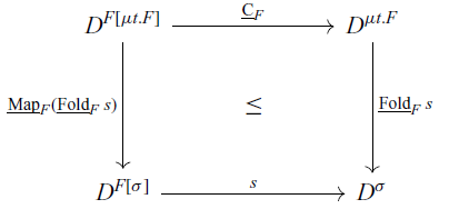
commute, where  $\underline{\mathrm{Map}}_F$ is a semantic function that corresponds to the $F[\cdot,\cdot]$ macro. Relative to the usual definition of initial algebra, this requirement is weak, in that we ask only for existence of a $\underline{\mathrm{Fold}}{}$ function making the diagram commute ( $\beta$ reduction) and not the uniqueness of $\underline{\mathrm{Fold}}{}$ ( $\eta$/induction), and it is lax, in that we ask that $\beta$-reduction holds only as an inequality, rather than an equality.
Nonetheless, under assumptions that turn out to be relatively easy to ensure, we can define  $\underline{\mathrm{Fold}}_{\Phi,U}$. Given a subset $X\subseteq A$ of a preordered set A, we say that $a\in A$ is a least upper bound of X, written $a = \bigvee X$, if for all $x\in X$, $x\leq a$, and if $b\in A$ satisfies the condition that for all $x\in X$, $x\leq b$, then $a\leq b$. When A is preordered, $\bigvee X$ may not exist, and when it does, it need not be unique. If A is a partial order (i.e., $a\leq b\leq a$ implies that $a=b$), then $\bigvee X$ is unique when it exists, and we say that A is a complete upper semi-lattice if A is a partial order and $\bigvee X$ exists for every $X\subseteq A$. Though this seems like a very strong condition, in practice it is easy to ensure.
In a model in which every  $D^U$ is a complete upper semi-lattice, we would like to define
 \[\underline{\mathrm{Fold}}_{\Phi,U}\,s\,x =\bigvee\{s\bigl(\Phi_{\mathord{\underline{\smash\mu}}\,\Phi,U}(\underline{\mathrm{Fold}}_{\Phi,U} s)\,z\bigr)\}{z\in D^{\Phi(\mathord{\underline{\smash\mu}}\,\Phi)}, {\underline{\mathrm{C}}_{\Phi}\,z \leq x}}.\tag{std-fold}\]
A priori, this definition may not be well founded, but in fact it is, as shown in the next proposition.
Proposition 3. Suppose that  ${\mathbf{U}} = \{D^U\}{U\in\mathbf{U}_{lg}}$ is a model of the fragment of the recurrence language that omits $\textsf{fold}_\delta$ and each $D^U$ is a complete upper semi-lattice, and suppose that $\underline{\mathrm{Fold}}$ is defined by (std-fold). Then:
1. For all s,
$\underline{\mathrm{Fold}}_{\Phi,U}\,s$ is total and monotone.-
2.
$\underline{\mathrm{Fold}}_{\Phi,U}$ is total and monotone.


1. Fix s and consider
\[ Q = {\lambda\hskip-.32em\lambda} g.{\lambda\hskip-.32em\lambda} x.\bigvee\{s\bigl(\Phi_{\mathord{\underline{\smash\mu}}\,\Phi,U}\,g\,z\bigr)\}{z\in D^{\Phi(\mathord{\underline{\smash\mu}}\,\Phi)}, \underline{\mathrm{C}}_{\Phi}\,z \leq x}.\]
$Q : (D^{\mathord{\underline{\smash\mu}}\,\Phi}\to D^U)\to(D^{\mathord{\underline{\smash\mu}}\,\Phi}\to D^U)$ and it is easy to see that Q is monotone. Since $D^U$ is a complete upper semi-lattice, $D^{\mathord{\underline{\smash\mu}}\,\Phi}\to D^U$ is a complete partial order. So Q has a least fixed point; that is, $\underline{\mathrm{Fold}}_{\Phi,U}\,s$.Footnote 4
Monotonicity of $\underline{\mathrm{Fold}}_{\Phi,U}\,s$ is immediate from its definition.
-
2. Totality follows from (1) and monotonicity from the fact that the function that maps a monotone function to its least fixed point is itself monotone.


The proof of Proposition 3, and hence the interpretation of  $\textsf{fold}_\delta$, may seem a bit heavy-handed, making use of general least fixed point theorems and even iterating into the transfinite. As we noted earlier, we are in a setting in which we do not have (and do not want) initial algebras, but must nonetheless show an initiality-like property of a given algebra. Accordingly, we would expect to use technology at least as strong as that needed for typical initial algebra existence theorems. The canonical such theorem (e.g., as described by Aczel Reference Aczel1988, Thm. 7.6) verifies that the least fixed point of a set-continuous operator is an initial algebra, and the verification consists of constructing the equivalent of $\underline{\mathrm{Fold}}\,s$ by induction on the (ordinal-indexed) construction of the least fixed point.
The reader may have noticed that an alternative possible definition for  $\underline{\mathrm{Fold}}$ is
 \[\underline{\mathrm{Fold}}\,s\,x= s(\Phi(\underline{\mathrm{Fold}}\,s)(\underline{\mathrm{D}}\,x))\]
and Proposition 3 would still hold. This fact witnesses that the initiality condition for  $\underline{\mathrm{C}}_{\Phi} : D^{\Phi(\mathord{\underline{\smash\mu}}\,\Phi)}\to D^{\mathord{\underline{\smash\mu}}\,\Phi}$ is weak, in that functions to other algebras are not unique. In practice, this alternative definition yields far worse bounds for extracted recurrences, because we end up defining $\underline{\mathrm{D}}_{\Phi}\,x = \bigvee\{z\}{\underline{\mathrm{C}}_{\Phi}(z)\leq x}$ and so $\underline{\mathrm{Fold}}\,s\,x= s(\Phi(\underline{\mathrm{Fold}}\,s)(\bigvee\{z\}{\underline{\mathrm{C}}_{\Phi}(z)\leq x}))$. Monotonicity of f only allows us to conclude that $f(\bigvee X) \geq\bigvee\{f(x)\}{x\in X}$, but this putative definition for $\underline{\mathrm{Fold}}\,s$ exposes a case in which this inequality is strict.
6.2 The standard type frame
Our last step in our general discussion of models is to define the type frame upon which all of our examples will be based. It gives us enough data to provide a standard definition of the functions  $\Phi_{U,V}$, which in turn lets us use (std-fold) to define $\underline{\mathrm{Fold}}$ and so for most of our examples, it will suffice to define $\underline{\mathrm{C}}_{\Phi}$ (because we will set $\underline{\mathrm{D}}_{\Phi} = \bigvee\{z\}{\underline{\mathrm{C}}_{\Phi}(z)\leq x}$). Our examples are all based on variations of the standard type frame, which is defined as follows:
•
$\mathbf{U}_{sm}$ is the set of closed types and $\mathbf{U}_{lg}$ the set of closed type schemes of the recurrence language.-
•
$\mathrel{\underline{\mathord\to}}$, $\mathrel{\underline{\times}}$, and $\mathrel{\underline{+}}$ are the standard type constructors; e.g., $\sigma_0\mathrel{\underline{+}}\sigma_1 = {\sigma_0}+{\sigma_1}$. -
•
$\mathrm{Dom}\;\mathord{\underline{\smash\mu}} = \{{\lambda\hskip-.32em\lambda}\sigma.F[\sigma]\}{\mathop{\mathrm{fv}}\nolimits(F) \subseteq \{t\}}$ and $\mathord{\underline{\smash\mu}}({\lambda\hskip-.32em\lambda}\sigma.F[\sigma]) = \mu t F$ (we call a structure functor F with $\mathop{\mathrm{fv}}\nolimits(F)\subseteq\{t\}$ closed). -
•
$\mathrm{Dom}\;\mathord{\underline{\forall}} = \{{\lambda\hskip-.32em\lambda}\sigma.\tau'\{\sigma/\alpha\}\}{\mathop{\mathrm{fv}}\nolimits(\tau)=\{\alpha\}}$ and $\mathord{\underline{\forall}}({\lambda\hskip-.32em\lambda}\sigma.\tau\{\sigma/\alpha\}) = \forall\alpha.\tau$.


It is straightforward to show that if  ${\lambda\hskip-.32em\lambda}\sigma.F[\sigma] ={\lambda\hskip-.32em\lambda}\sigma.F'[\sigma]$, then $F = F'$, and if ${\lambda\hskip-.32em\lambda}\sigma.\tau\sigma\mapsto\alpha = {\lambda\hskip-.32em\lambda}\sigma.{\tau'}\{\sigma/\alpha\}$, then $\tau = \tau'$, so $\mathord{\underline{\smash\mu}}$ and $\mathord{\underline{\forall}}$ are well defined. It should be clear and occasionally helpful to observe that for any $\tau$ and environment $\eta =\{\alpha_0\mapsto{\sigma_0},\dots,{\alpha_{n-1}}\mapsto{\sigma_{n-1}}\}$, $[\![\tau]\!]\eta = \tau\{\vec{\sigma}/\vec{\alpha}\}$. For models based on the standard type frame and any closed structure functor F, we will usually write F in place of ${\lambda\hskip-.32em\lambda}\sigma.F[\sigma]$ in subscripts for readability.
Proposition 4. The standard type frame is a type model.
For any applicative structure based on (an extension of) the standard type frame, define  $F_{\rho,\sigma} : (D^\rho\to D^\sigma)\to(D^{F[\rho]}\to D^{F[\sigma]})$ for each closed structure functor F and closed $\rho$ and $\sigma$ by
 \[\begin{aligned}[t]t_{\rho,\sigma}\,g\,x &= g\,x \\(\sigma_0)_{\rho,\sigma}\,g\,x &= x \\\end{aligned}\qquad\begin{aligned}[t]({F_0}+{F_1})_{\rho,\sigma}\,g\,x &= \underline{\mathrm{Case}}(x, {\lambda\hskip-.32em\lambda} y.\underline{\mathrm{Inj}}^0((F_0)_{\rho,\sigma}\,g\,y),{\lambda\hskip-.32em\lambda} y.\underline{\mathrm{Inj}}^1((F_1)_{\rho,\sigma}\,g\,y)) \\({F_0}\times{F_1})_{\rho,\sigma}\,g\,x &= \underline{\mathrm{Pair}}((F_0)_{\rho,\sigma}\,g\,(\underline{\mathrm{Proj}}^0 x),(F_1)_{\rho,\sigma}\,g\,(\underline{\mathrm{Proj}}^1 x)),\\({\sigma_0}\to{F})_{\rho,\sigma}\,g\,x &= {\lambda\hskip-.32em\lambda} y.F_{\rho,\sigma}\,g\,(x\,y)\end{aligned}\]
Lemma 7. If  ${\mathbf{U}}$ is an applicative structure based on an extension of the standard type frame that is a model for the fragment of the recurrence language that omits $\textsf{fold}_\delta$, ${\Gamma,y\mathbin:\rho}\vdash{e'}:{\sigma}$, $\Gamma\vdash e: {F[\rho]}$, and $\eta$ is a $\Gamma$-environment, then
 \[ [\![{F [(\rho:y).{e'}, e]}]\!]\eta = ([\![ F]\!]\eta)_{[\![\rho]\!]\eta,[\![\sigma]\!]\eta}\,({\lambda\hskip-.32em\lambda} a.[\![{e'}]\!]\eta\{y\mapsto a\} )\,([\![ e]\!] \eta).\]
Proof. By induction on F.
Combining Proposition 3 with Lemma 7, we conclude that to define a model of the recurrence language, it suffices to define an extension of the standard type frame and the following applicative structure data:
• The sets
$D^\tau$, along with an argument that $D^\tau$ is a complete upper semi-lattice;-
• The semantic functions for arrow, product, and sum types;
-
•
$\underline{\mathrm{C}}_{F}$ for each structure functor F.


From this data, we can define  $\underline{\mathrm{D}}_F(x) = \bigvee\{z\}{\underline{\mathrm{C}}_{F}\leq x}$, $F_{\rho,\sigma}$ as just given, and $\underline{\mathrm{Fold}}_{F,\sigma}$ by (std-fold). Of course, there are models that are not constructed this way; Section 7.5 gives an example that is useful for extracting recurrences for lower bounds.
6.3 Syntactic sugar
We now introduce some syntactic sugar that will make our discussion of recurrences somewhat more pleasant. To simplify the discussion, we restrict the details to the source language type  $\sigma\mathtt{tree}$ and its recurrence language potential $\sigma\mathtt{tree}$, but we will use analogous notation for other datatypes such as $\mathtt{nat}$ and $\alpha\mathtt{list}$ in our examples. Many of our source-language functions are really structural folds over some standard datatype—that is, the step function is a $\mathtt{case}$ expression where the argument for each branch is really the argument to one of the datatype constructors. Accordingly, we introduce notation for such $\mathtt{fold}$ expressions: for $y\notin\mathop{\mathrm{fv}}\nolimits(e_\mathtt{emp})\cup\mathop{\mathrm{fv}}\nolimits(e_\mathtt{node})$,
 \[\mathtt{fold}_{\sigma\mathtt{tree}} e \mathtt{of emp}\Rightarrow {e_\mathtt{emp}}|\mathtt{node}\Rightarrow {(x, r_0, r_1).e_\mathtt{node}}\]
is syntactic sugar for
 \[\mathtt{fold}_{\sigma \mathtt{tree}} e \mathtt{of} w.{\mathtt{case} w \mathtt{of} y.{e_\mathtt{emp}}; y.{e_\mathtt{emp}; {y.e_\mathtt{node}} {\pi_0 y, \pi_1 y, \pi_2 y} {x, r_0, r_1}}}.\]
We introduce a similar notation in the recurrence language:
 \[\mathtt{fold}_{\sigma \mathtt{tree}} e \mathtt{of} \{\textsf{emp}\Rightarrow e_\textsf{emp}|\textsf{node}\Rightarrow (x, r_0, r_1).e_\textsf{node}\}\]
is syntactic sugar for
 \[\mathtt{fold}_{\sigma \mathtt{tree}} e {(w : {F_{\sigma\mathtt{tree}}}[\rho]).} {{(\textsf{Case} w \textsf{of}y.{e_\textsf{emp}};y.{{e_{\textsf{node}}} {\pi_0 y, \pi_1 y, \pi_2 y}/{x, r_0, r_1}})}}\]
where w and y are fresh variables.
It would be nice to establish an identity of the form  $\|{\mathtt{fold}_{\sigma\mathtt{tree}}\dotsb}\| = \textsf{fold}_{\sigma\textsf{tree}}\dotsb$, but the size-order axioms, which give us only inequalities, are too weak. However, the models that we will consider validate many equations, so we can set out a nice relationship. In the following proposition, we say “in the semantics, $e = e'$” to mean that for any $\eta$, $[\![ e]\!]\eta = [\![ {e'}]\!] \eta$:
Proposition 5 Suppose that we have a model such that
• In the semantics: if
$\|{{e'}}\|_c = 0$, then $\|e\{e'/x\}\| = {\|e\|} {{\|e'\|}_p}/x$; and-
• In the semantics:
$c+_c {\textsf{case} e \textsf{of} \{x.e_i\}}_{i=0,1} = \textsf{case} e \textsf{of}\{x.c+_{c}e_{i}\}_{i=0,1}$.


If  $\Gamma\vdash\textsf{fold}_{\sigma\textsf{tree}} e \textsf{of\,emp}\Rightarrow {e_\mathtt{emp}}|\textsf{node}\Rightarrow(x,r_{0},r_{1}).e_{\textsf{node}}:\rho$, then in the semantics,
 \begin{multline*}\|\mathtt{fold}_{\sigma\mathtt{tree}} e \textsf{of\,emp}\Rightarrow\,e_{\textsf{emp}}|\textsf{node}\Rightarrow(x,r_{0},r_{1}).e_{\textsf{node}}\|=c+_{c}\textsf{fold}_{\sigma\mathtt{tree}}p\textsf{of} \{\textsf{emp}\Rightarrow1+_{c}\|E_{\textsf{emp}}\| |\textsf{node}\Rightarrow(x,r_{0},r_{1}).1+_{c} \|E_{\textsf{node}}\|\}\end{multline*}
where  $(c, p) = \|e\|$.
While the models that we discuss in subsequent sections satisfy the hypotheses of Proposition 5, they are not necessarily satisfied in an arbitrary model. That requires additional axioms that correspond roughly to  $\eta$ axioms.
7 Examples
7.1 The standard model
For the standard model, we first extend the standard type frame by including the constant  $\bot$ in $\mathbf{U}_{sm}$. A semantic type (scheme) is proper if it has no occurrences of $\bot$. The proper semantic types (type schemes) correspond exactly to the closed syntactic types (type schemes). In the definitions of $\mathord{\underline{\smash\mu}}$ and $\mathord{\underline{\forall}}$, we take F and $\tau$ to be proper. We define the sets $A^\sigma$ by induction on $\sigma$ as follows:Footnote 5
-
•
$A^\textsf{C} = \mathbf{N}$, the natural numbers. -
•
$A^\bot = \emptyset$. -
•
$A^{\textsf{unit}} = \{*\}$, some one-element set. -
•
$A^{{\sigma_0}\to{\sigma_1}} = (A^{\sigma_1})^{A^{\sigma_0}}$, the set of functions from $A^{\sigma_0}$ to $A^{\sigma_1}$. -
•
$A^{{\sigma_0}\times{\sigma_1}} = A^{\sigma_0}\times A^{\sigma_1}$, where $\times$ is the standard set-theoretic product. -
•
$A^{{\sigma_0}+{\sigma_1}} = A^{\sigma_0}\sqcup A^{\sigma_1}$, where $\sqcup$ is the standard set-theoretic disjoint union. -
•
$A^{\mu t.F} = \bigcup_i A^{({\lambda\hskip-.32em\lambda} V.[\![ F]\!] {\{t\mapsto V\}})^i\bot}$. -
•
$A^{\forall\alpha\tau} = \prod_{\sigma\in\mathbf{U}_{sm}} A^{\tau\{\sigma/\alpha\}}$.


Define  $a\leq_{A^\sigma} b$ iff $a=b$, and let the semantic functions for arrows, products, and sums be the identity functions. The definitions of $\underline{\mathrm{C}}_{F}$, $\underline{\mathrm{D}}_F$, and $\underline{\mathrm{Fold}}_{F,\sigma}$ are based on the standard initial-algebra semantics. Note that we cannot use (std-fold) because the $A^\sigma$ are not complete upper semi-lattices, and hence the hypotheses of Proposition 3 do not hold, and hence $\beta_{\delta\textsf{fold}}$ must be verified directly.
At first blush, this model is not particularly interesting. There is no abstraction of values to sizes and the “order” on costs is the identity, so the recurrences extracted from source language programs describe the exact cost of those programs in terms of the argument values. However, this is a standard model of (predicative) polymorphism, and so we can hope that parametricity may have some interesting consequences. Free theorems (Wadler Reference Wadler1989) have been used to obtain relative cost information, and we discuss this further in Section 9. Here, we apply parametricity to the recurrence language and sketch the argument that if  $g: {\alpha\mathtt{list}}\rightarrow{\alpha\mathtt{list}}$, then the cost of g(xs) depends only on the length of xs (the same can be said for the length of g(xs), but this follows from parametricity applied to the source language). For any $\rho$, let us define $T_\rho(xs) =(([\![{\|g\|}]\!]{}\,\langle\langle\rho\rangle\rangle)_p(xs))_c$, the exact cost of evaluating g(xs) (since $\|\cdot\|$ is a monadic translation and the interpretation of inductive types is the standard one, syntactic values of list type in the source language are isomorphic to the semantic values in the model). The goal is to show that if $xs : \rho\mathtt{list}$ and $ys : \sigma\mathtt{list}$ are of the same length, then $T_\rho(xs) =T_\sigma(ys)$. To do so, we apply parametricity to ${\lambda\hskip-.32em\lambda} \rho.{\lambda\hskip-.32em\lambda} xs.T_\rho(xs) \in A^{\forall \rho.\rho\mathtt{list} \to \textsf{C}}$. We take the relational interpretation of $\textsf{C}$ to be equality (so the cost constants 0 and $+$ preserve the relation). Expanding the definition of parametricity, this means that for any $\rho$ and $\sigma$ and relation $R \subseteq A^{\langle\langle\rho\rangle\rangle}\times A^{\langle\langle\sigma\rangle\rangle}$, for any $xs \in A^{{\langle\langle\rho\rangle\rangle}\textsf{list}}$ and $ys \in A^{\langle\langle\sigma\rangle\rangle\textsf{list}}$, if $R\textsf{list}\subseteq A^{{\langle\langle\rho\rangle\rangle}\textsf{list}}\times A^{\langle\langle\sigma\rangle\rangle\textsf{list}}$ holds for xs and ys, then the relational interpretation of $\textsf{C}$ holds for $T_\rho(xs)$ and $T_\sigma(ys)$. Since the relational interpretation of the cost type is equality, this would give the result, so it suffices to show that there is an R such that $(R\textsf{list})(xs,ys)$ holds whenever xs and ys have the same length. However, the standard relational lifting $R\textsf{list}$ holds whenever xs and ys have the same length and $xs_i$ is related to $ys_i$ by R, so taking R to be the total relation achieves this. We conclude that if xs and ys have the same length, then the cost of g(xs) and g(ys) is the same.
7.2 Constructor size and height
We now describe a model in which a value v of inductive type  $\delta$ is interpreted either by the number of $\delta$ constructors in v (constructor size) or by the maximum nesting depth of $\delta$-constructors in v (constructor height), so that it reflects common size abstractions such as list length, tree size, and tree height. For example, in this model, the interpretation of the recurrence extracted from a function with domain $\sigma\textsf{list}$ describes the cost in terms of the length of the argument list. For concreteness we will define the constructor size model. For the interpretation of the types, we will need two versions of the natural numbers: $\mathbf{N}_0^\infty = \{0,1,\dots,\infty\}$ for costs, and $\mathbf{N}_1^\infty = \{1,2,\dots,\infty\}$ for sizes of inductive values, which must be at least 1 because every value contains at least one constructor. $\mathbf{N}_i^\infty$ is ordered by $x\leq_{\mathbf{N}_i^\infty} y$ if $y=\infty$ or $x\leq_\mathbf{N} y$. The presence of $\infty$ may be perplexing, since all programs in the source language terminate. However, it is not always possible to give a finite upper bound on cost or potential in terms of the potential of the argument, because the notion of potential used in this model may not identify all possible sources of recursive calls. For example, consider the function $\mathtt{sumtree}$ defined in Figure 22 that sums the nodes of a $\mathtt{nat tree}$. The cost and size of $\mathtt{sumtree}\,t$ depend on the size of t and the sizes of its labels, whereas in this model, the potential of t only tells us the former. Since $\mathtt{sumtree}$ is definable in our source language, its recurrence can be extracted, and hence must have a meaning in this model; the only sensible interpretation is one that maps every tree size to the trivial upper bound of $\infty$ for both cost and potential.

Fig. 21. Binary search tree membership and its extracted recurrence.

Fig. 22. A function that sums the nodes of a  $\mathtt{nat tree}$.
We start by extending the standard type frame with additional small types  $\mathbf{N}_0,\mathbf{N}_1\in\mathbf{U}_{sm}$. Then we define the sets $V^\tau$, observing that each $V^\tau$ is a complete upper semi-lattice. This allows us to construct a model by just defining $\underline{\mathrm{C}}_{F}$. The sets $V^\tau$ are defined as follows:
•
$V^{\mathbf{N}_i} = \mathbf{N}_i^\infty$.-
•
$V^\textsf{C} = \mathbf{N}_0^\infty$ with the standard interpretations for $\underline{0}$ and $\underline{+}$, where $x\mathbin{\underline{+}}\infty =\infty\mathbin{\underline{+}}x = \infty$. -
•
$V^\textsf{unit} = \{*\}$. -
•
$V^{{\sigma_0}\to{\sigma_1}} =$ the set of monotone functions from $V^{\sigma_0}$ to $V^{\sigma_1}$ with the usual pointwise order, taking $\underline{Abs}$ and $\underline{App}$ to be the identity functions. -
•
$V^{{\sigma_0}\times{\sigma_1}} =V^{\sigma_0}\times V^{\sigma_1}$ with the usual component-wise order, taking $\underline{\mathrm{Pair}}$ and $\underline{\mathrm{Proj}}$ to be the standard pairing and projection functions. -
•
$V^{{\sigma_0}+{\sigma_1}} =\mathcal{O}(V^{\sigma_0}\sqcup V^{\sigma_1})$, which we define in Section 7.2.1. -
•
$V^{\mu t F} = \mathbf{N}_1^\infty$. We define $\underline{\mathrm{C}}_{F}$ in Section 7.2.2 (recall that we write $\underline{\mathrm{C}}_{F}$ for $\underline{\mathrm{C}}_{{\lambda\hskip-.32em\lambda} V.[\![ F]\!] \{V/t\}}$, etc., and that we can define $\underline{\mathrm{D}}_F$ and $\underline{\mathrm{Fold}}_{F,\sigma}$ from it). -
•
$V^{\forall\alpha.\tau} =\prod_{\sigma\in\mathbf{U}_{sm}}V^{\tau\{\sigma\alpha\}}$, with the pointwise order, taking $\underline{TyAbs}$ and $\underline{TyApp}$ to be the identity functions.


Once we define the interpretation of sums and datatypes, it is straightforward to verify that this is a model.
Proposition 6  $\mathbf{V} = \{V^\tau\}{\tau\in\mathbf{U}_{lg}}$ is a model of the recurrence language.
Proof. Since  $\underline{Abs}$ and $\underline{TyAbs}$ are total, it suffices to verify the conditions on the semantic functions. This is trivial for arrows, products, and type quantification; sums and inductive types are handled in the next two sections. ■
7.2.1 Interpretation of sums
As we observed, we need to ensure that all the sets  $V^\sigma$ are complete upper semi-lattices. Preserving the complete upper semi-lattice property is straightforward for all type constructors except sum. We could take the usual disjoint sum along with a new infinite element $\infty$ that is a common upper bound of elements on both sides, but that ends up leading to very weak bounds in practice. For example, recall that $\underline{\mathrm{D}}_{\sigma\textsf{list}}(2)$ should tell us about the data that can be used to construct a list of size $\leq 2$ (which is a $\textsf{cons}$ list, because we count the number of $\textsf{c}_{\sigma\textsf{list}}$ constructors, so $\textsf{nil}$ has size 1). If we were to interpret sums as just proposed, both $\underline{\mathrm{Inj}}^0(*)$ and $\underline{\mathrm{Inj}}^1(a, 0)$ are such values, and their least upper bound would be $\infty$. It is not hard to parlay this into an argument that if $\mathtt{tail} = \lambda{xs}.{\mathtt{case}{xs} \mathtt{of} {x}.{\mathtt{nil}}; {x}.{\pi_1 x}}$ is the usual tail function on $\sigma\mathtt{tree}$, then the recurrence extracted from $\mathtt{tail}$ gives a bound of $\infty$ for all lists of length $>1$. While correct, this is hardly satisfying!
Instead, we take inspiration from abstract interpretation (Cousot & Cousot Reference Cousot and Cousot1977): we will define  $\underline{\mathrm{D}}_F(n)$ to be the set of values x such that $\underline{\mathrm{C}}_{F}(x)\leq n$. We can arrange this for the typical cases of interest (i.e., finitary inductive datatypes such as lists and trees) by defining $V^{{\sigma_0}+{\sigma_1}}$ to be the downward closed subsets of $V^{\sigma_0}\sqcup V^{\sigma_1}$. We could arrange this for all inductive datatypes if we were to do something similar in the interpretation of arrows and products, but that entails some additional notational cost in reasoning about extracted recurrences while providing no benefits for the examples that we present. We start with some standard order-theoretic and set-theoretic definitions:
• For any partially ordered set A, the order ideal of A is
\[\mathcal{O}(A) =_{df}\{X\subseteq A\}{\text{$x\in X$ and $y\leq x$}\Rightarrow y\in X}.\]
$\mathcal{O}(A)$ is partially ordered by set inclusion and is a complete upper semi-lattice; concretely, if $X\subseteq\mathcal{O}(A)$, then $\bigvee X = \bigcup X$.
-
• For any
$X\subseteq A$, $X\subseteq A,\downarrow^{A} X= \{x\in A\}|{\exists y\in X.x\leq y}\in\mathcal{O}(A)$ and for $a\in A$, $\downarrow^{A} a = \downarrow^{\{a\}}$ (we drop the superscript when it is clear from context). -
• For any
$f : A \to B$ and $X\subseteq A$, $f[X] = \{f(x)\}{x\in X}$. -
• If
$X_0$ and $X_1$ are partially ordered sets, $X_0\sqcup X_1$ is the usual disjoint union with injection functions $\mathrm{in}^{i}:X_i\to X_0\sqcup X_1$ partially ordered by $x\leq y$ iff $x = \mathrm{in}^{i}(x')$, $y = \mathrm{in}^{i}(y')$, and $x'\leq_{X_i} y'$.


For the interpretation of sums, we define  $V^{{\sigma_0}+{\sigma_1}} =\mathcal{O}(V^{\sigma_0}\sqcup V^{\sigma_1})$ with the semantic functions defined by
 \begin{align*}\underline{\mathrm{Inj}}^i(x) &= \mathrm{in}^{i}[\downarrow^{V}{^{\sigma_i}} x] = [\downarrow^{V}{^{\sigma_0}}\sqcup V^{\sigma_1}](\mathrm{in}^{i}(x)) \\\underline{\mathrm{Case}}(X_0\sqcup X_1, f_0, f_1) &= \bigvee f_0[X_0] \vee \bigvee f_1[X_1]\end{align*}
Lemma 8  $\underline{\mathrm{Case}}(\underline{\mathrm{Inj}}^i(x), f_0, f_1) \geq f_i(x)$.
 \begin{align*}\underline{\mathrm{Case}}(\underline{\mathrm{Inj}}^i(x), f_0, f_1) &= \underline{\mathrm{Case}}(\mathrm{in}^{i}[\downarrow x]\sqcup\emptyset, f_0, f_1) \\ &= \bigvee f_i[\downarrow x] \vee \bigvee f_{1-i}[\emptyset] \\ &= \bigvee f_i[\downarrow x] \\ &\geq f_i(x) & & (x\in\downarrow x).\end{align*}
Note that  $\mathcal{O} A$ is a monad on the category of partially ordered sets and monotone functions, with unit $A \to \mathcal{O} A$ given by $\downarrow^A$, and multiplication $\mathcal{O} {\mathcal{O} A} \to\mathcal{O} A$ given by union, and it plays the role of a powerset monad on posets (the ordinary powerset operation, without the additional downward closure requirement, does not have a monotone function $A \to \mathcal{P}(A)$, because $x \leq_A y$ does not imply that $\{x\}\subseteq\{y\}$. When a partially ordered set is a complete upper semilattice (i.e. supports the maximum operation that we use to interpret the recursor), it is an algebra for this monad, i.e. there is a monotone function $\mathcal{O} A \to A$, satisfying some equations. Thus, another way of understanding these models is that, for functions and products, we build algebras $\bigvee_{A\to B} : \mathcal{O}(A \to B) \to (A \to B)$ and $\bigvee_{A\times B} : \mathcal{O}(A \times B) \to A \times B$ from algebra structures $\bigvee_{A} : \mathcal{O} A\to A$ and $\bigvee_B : \mathcal{O} B \to B$, but for sums, we use the free algebra $\mathcal{O}(A + B)$, with $\bigvee_{\mathcal{O}(A + B)} :\mathcal{O}{\mathcal{O} (A + B)} \to \mathcal{O}{(A+B)}$ given by union.
7.2.2 Semantic functions for inductive datatypes
We define  $\underline{\mathrm{C}}_{F}$ by first defining a function $\underline{\mathrm{size}}_{F} : V^{[F {\mu t.F}]}\to \mathbf{N}_0^\infty$. For $\delta = \mu t F$, a semantic value of type ${F[{\mu t.F}]}$ represents the data from which a value of type $\delta$ is constructed, but with the inductive substructures replaced by their sizes, and $\underline{\mathrm{size}}_{F}$ returns the size of the inductive value constructed from that data.
 \[\begin{aligned}[t]\underline{\mathrm{size}}_{t}(n) &= n \\\underline{\mathrm{size}}_{\sigma}(x) &= 0\end{aligned}\qquad\begin{aligned}[t]\underline{\mathrm{size}}_{{F_0}+{F_1}}{}(X_0\sqcup X_1) &= \bigvee\underline{\mathrm{size}}_{F_0}[X_0]\vee\bigvee\underline{\mathrm{size}}_{F_1}[X_1] \\\underline{\mathrm{size}}_{{F_0}\times{F_1}}(a_0, a_1) &= \underline{\mathrm{size}}_{F_0}{}(a_0) + \underline{\mathrm{size}}_{F_1}(a_1) \\\underline{\mathrm{size}}_{{\sigma}\to{F}}(g) &= \sum\{\underline{\mathrm{size}}_{F}(g\,x)\}{x\in V^\sigma}\end{aligned}\]
For the constructor height model, define a function  $\underline{\mathrm{height}} F$ analogously, replacing the sums in the product and arrow shapes with maximums. The semantic constructor and destructor are then defined by
 \[\underline{\mathrm{C}}_{F}(a) = 1 + \underline{\mathrm{size}}_{F}(a)\qquad\underline{\mathrm{D}}_F(n) = \bigvee\{a\}{\underline{\mathrm{C}}_{F}\,a \leq n}.\]
To use (std-fold), it suffices to verify the conditions of Proposition 3, which is trivial, so we have
 \[\underline{\mathrm{Fold}}_{F,\sigma}\,s\,x =\bigvee\{s\bigl(F_{\delta,\sigma}(\underline{\mathrm{Fold}}_{F,\sigma}\,s)z\bigr)\} {1 + \underline{\mathrm{size}}_{F}(z) \leq x}.\]
7.2.3 Examples: lists and trees
Referring to Figure 10,

It is not hard to see that  $[\![{\_\vdash t {\sigma\textsf{tree}}}]\!]{} = 2n + 1$, where n is the usual size of t (i.e., $[\![{\_\vdash t {\sigma\textsf{tree}}}]\!]{}$ is the number of internal and external nodes of t). Since this is linear in the usual notion of size of a tree, it suffices for showing that the recurrences that we extract have the expected O-behavior.
Destructors exhibit the desired behavior; consider  $\sigma\textsf{list}$ again:
 \begin{align*}\underline{\mathrm{D}}_{F_{\sigma\textsf{list}}}(x) &= \begin{cases} \{*\}\sqcup\emptyset,&x=1 \\ \{*\}\sqcup\{(a, x')\} {a\in V^\sigma, 1+x'\leq x},&2\leq x \leq \infty \end{cases} \\ &= \{*\}\sqcup (V^\sigma\times \downarrow^{\mathbf{N}_1^\infty}(x-1))\end{align*}
where we define  $\downarrow^{\mathbf{N}_1^\infty}0 = \emptyset$. In other words, a list of size 1 must be $\mathtt{nil}$ and a list of length at most x is either $\mathtt{nil}$ or $\mathtt{cons}(x, xs)$, where xs has length at most $x-1$. Remember that $V^{F {[\sigma\textsf{list}]}} =\mathcal{O}(\{*\}\sqcup (V^\sigma\times\mathbf{N}_1^\infty))$, so if $\mathrm{in}^{l}(a, x)\in X\in V^{F{[\sigma\textsf{list}]}}$, then $x\geq 1$; that is why $\underline{\mathrm{D}}_{F_{\sigma\textsf{list}}}(1)\not=\{*\}\sqcup X$ with $X\not=\emptyset$. For $\sigma\textsf{tree}$, the result is equally pleasant:
 \[\underline{\mathrm{D}}-{F_{\sigma\textsf{tree}}}(x) =\begin{cases}\{*\}\sqcup\emptyset,&x=1 \\\{*\}\sqcup\{(a, x_0, x_1)\} {a\in V^\sigma, 1+x_0+x_1\leq x},&2\leq x \leq \infty\end{cases}\]
Finally, we observe the following simple forms for the denotation of recurrences over lists and trees:
1. If
$f\,n=[\![\textsf{fold}_{\sigma\textsf{list}}y\textsf{of}\{\textsf{nil}\Rightarrow e_{\textsf{nil}}|\textsf{cons}\Rightarrow(x,r).e_{\textsf{cons}}\}]\!]\eta\{y\mapsto n\}$, then in the constructor size and height models,
The second form for
\begin{align*}f\,1 &= [\![{e_\textsf{nil}}]\!]\eta \\f\,n &= [\![{e_\textsf{nil}}]\!]\eta \vee \bigvee\{[\![{e_\textsf{cons}}]\!] \eta \{x, r\mapsto \infty^\sigma, f\,n' \}| \}|{n'
< n} \\ &= [\![{e_\textsf{nil}}]\!]\eta \vee [\![{e_\textsf{cons}}]\!] \eta \{x, r\mapsto \infty^\sigma, f(n-1)\} & & (n > 1).\end{align*}
$f\,n$, $n>1$, follows from monotonicity of the denotation function.
-
2. If
$f\,n=[\![\textsf{fold}_{\sigma\textsf{tree}}y\textsf{of}\{\textsf{emp}\Rightarrow e_{\textsf{emp}}|\textsf{node}\Rightarrow(x,r_0,r_1).e_{\textsf{node}}\}]\!]\eta\{y\mapsto n\}$, then in the constructor size model,
In the constructor height model, replace
\begin{align*}f\,1 &= [\![{e_\textsf{emp}}]\!]\eta \\f\,n &= [\![{e_\textsf{emp}}]\!]\eta \vee \bigvee\{[\![{e_\textsf{node}}]\!] \eta \{x, r_0, r_1\mapsto \infty^\sigma, f\,n_0, f\,n_1 \} \}{n_0+n_1
< n} & & (n > 1).\end{align*}
$n_0+n_1 < n$ with $n_0\vee n_1 < n$.


Proof. The verification is a moderately tedious calculation; here, it is for (2) with  $n>1$. Let

Observe that  $f = \underline{\mathrm{Fold}}\,s$ and let us write $\underline{\mathrm{Map}}$ for $([\![{F_{\sigma\textsf{tree}}}]\!]{\eta})_{[\![{\sigma\textsf{tree}}]\!]\eta,[\![\rho]\!]\eta}$. By definition, we have $ f{\mkern 1mu} n = \bigvee \{ s(\underline {{\rm{Map}}} {\mkern 1mu} f{\mkern 1mu} (Z \sqcup X))|\underline {\rm{C}} (Z \sqcup X) \le n\} $. By monotonicity, we need only consider $Z = \{*\}$, and by definition of $\underline{\mathrm{C}}$, we need only consider nonempty sets X such that $(\underline{~}, n_0, n_1)\in X$ implies $n_0+n_1 < n$, so

Let us write the last equation as
First, let us show that for any X such that  $(\underline{~},n_0,n_1)\in X\Rightarrow n_0+n_1 < n$, $A_X\subseteq\downarrow B$, from which we conclude that $\bigvee A_X\leq\bigvee B$, and hence $L\leq R$. For any such X, take $(b, k_0, k_1)$ such that there is $(a, n_0, n_1)\in X$ with $(b, k_0, k_1)\leq (a, f\,n_0, f\,n_1) \leq(\infty,f\,n_0, f\,n_1)$. By Proposition 6, $[\![{e_\textsf{node}}]\!]{\eta\{x,r_0,r_1\mapsto b,k_0,k_1\}} \leq[\![{e_\textsf{node}}]\!]{\eta\{x,r_0,r_1\mapsto\infty,f\,n_0,f\,n_1\}}$. Since $(b, k_0, k_1)$ was chosen arbitrarily, $A_X\subseteq\downarrow B$, as needed. To show that $R\leq L$, suppose that $n_0+n_1<n$. Then $[\![{e_\textsf{node}}]\!]{\eta\{x,r_0,r_1\mapsto\infty,f\,n_0,f\,n_1\}} \in A_{\downarrow(\infty,n_0, n_1)}$, from which $R\leq L$ follows. ■
Although we will primarily use Proposition 7, it may be instructive to work through an example of explicitly constructing  $\underline{\mathrm{Fold}}_{F,\rho}$ from the proof of Proposition 3. Consider $F = \textsf{unit} +t$ (the structure functor for $\textsf{nat}$) and set $s(x) = \underline{\mathrm{Case}}(x, {\lambda\hskip-.32em\lambda} u.1, {\lambda\hskip-.32em\lambda} u.1+x)$. s might be the step function for the recurrence that describes the cost of the copy function on $\mathtt{nat}$. Define Q as in the proof of Lemma 3. In this setting, the bottom element at which we start iterating Q is the function that is constantly 0. Set $f_0 = Q\,\bot$ and $f_{n+1} = Q\,f_n$. Just as in the calculation of $\underline{\mathrm{D}}_{F_{\sigma\textsf{list}}}$,
 \[\underline{\mathrm{D}}{F_\textsf{nat}}(x) =\begin{cases}\{*\}\sqcup\emptyset,&x=1 \\\{*\}\sqcup\{x'\}{1+x'\leq x},&2\leq x\end{cases}\]
and so a bit more calculation shows that
 \[f_k(n) =\begin{cases}n,& n\leq k+1 \\k+1,& n>k+1.\end{cases}\]
It is not hard to see that  $f_{\omega(n)} = n$ is a fixed point of Q, so we conclude that $[\![\mathsf{fold_{nat}}x \mathsf{of} \{Z\Rightarrow 1\mid\mathsf{S}\Rightarrow r.\mathsf{S}r\}]\!]{{x\mapsto n}} = n$.
Of course, this is precisely what we expect, though for readers familiar with how a typical recursive function on numbers is defined by successive approximations, the route may feel a bit different. Usually when defining a recursive function on numbers, one takes the flat order and starts with the everywhere-undefined function. For a typical total function, the kth approximation is a partial function that is defined and correct on some initial segment of the natural numbers and undefined elsewhere. Here we take the (more-or-less) standard order and start with a function that is everywhere an unlikely bound (namely, 0). Each successive approximation yields a function with more likely bounds, terminating with a (hopefully low but) correct bound. In the case of a partial recursive function, the “bad” case is that the function is not defined for some numbers (the value of the approximants never gets above  $\bot$). In our setting, the “bad” case is that the bound is infinite (the value of the approximants never stops growing). The reader may wish to compare this with the use of $\mathbf{N}_0^\infty$ by Rosendahl (Reference Rosendahl1989), where $\infty$ corresponds to the bottom element in the usual CPO semantics for fixpoints. We return to this in Section 8 when we discuss general recursion.
7.2.4 Example: tree copy
For a first “sanity check,” let us analyze the tree copy function that is defined in Figure 20. We will also describe some of the main features in the analysis that are typical of all of our examples. The first is that a source language program  $e = \lambda{x,y,z}{e'}$ extracts to a recurrence of the form $(0, \lambda x.(0, \lambda y.(0, \lambda z.\|e'\|)))$. However, we are really only interested in $\|e'\|$ as a function of the potentials x, y, and z. Accordingly, when analyzing a program such as e, we focus on the recurrence language program $\lambda{x,y,z}{\|e'\|}$. Here, this means we will analyze the (denotation of the) recurrence $\textsf{copy}_{\sigma\textsf{tree}}$ that is also shown in Figure 20. Second, we shall use Proposition 5 freely as though it is a theorem about the syntax when we write our examples. Third, in our examples, we typically use the identifier r in syntactic recurrences for a recursive call to the computation of a complexity, and hence $r_p$ and $r_c$ correspond to recursive calls that compute potential and cost, respectively. Finally, we remind the reader that our goal is to show that the semantic recurrences are essentially the same as those that we expect to arise from an informal analysis, and so we make no attempt to solve them.
The analysis for  $\mathtt{copy}_{\sigma\mathtt{tree}}$ proceeds as follows. Define $T(n) = ([\![{\textsf{copy}_{\sigma\textsf{tree}}}]\!]{}(n))_c$. Following the definition of the denotation function and using Proposition 7 and facts about $\vee$ and $\bigvee$ in the semantics, we have
 \[T(1) = 1\qquad\begin{aligned}[t]T(n) &= 1 \vee \bigvee\{1 + T(n_0) + T(n_1)\}{n_0+n_1<n} \\ &= \bigvee\{1 + T(n_0) + T(n_1)\}{n_0+n_1<n}\end{aligned}\]
and we obtain a similar recurrence for  $S(n) = ([\![{\textsf{copy}_{\sigma\textsf{tree}}}]\!]{}(n))_p$. We observe that these are precisely the expected recurrences from an informal analysis which, if one is careful, must consider all possible combinations of subtree sizes when computing the cost or size of the result when the argument tree has size n.
7.2.5 Example: binary search tree membership
For an interesting example, let us consider membership testing in  $\sigma$-labeled binary search trees. First, we define the type
 \[\mathtt{order} = {\mathtt{unit}+\mathtt{unit}}+\mathtt{unit}\]
and write  $\mathtt{case}\,e\,\mathtt{of}\,\mathtt{LT}.{e_0}; \mathtt{EQ}.{e_1};\mathtt{GT}.{e_2}$ for $\mathtt{case}^\mathtt{order}\,e\,\mathtt{of}\,x.e_0; x.e_1; x.e_2$, and we assume comparable notation in the recurrence language. The membership test function is given in Figure 21.
Let us consider an informal analysis of  $\mathtt{mem}$, which is somewhat simpler to describe in reference to the $\mathtt{member}$ function of Figure 8(a). Let T(h) be the number of calls to $\mathtt{member}$ in terms of the height of t. We would probably argue that $T(1) = 1$ and for $h>1$,
 \[T(h) \leq \underbrace{1}_{\text{the call to $\mathtt{member}$}} +\underbrace{\bigvee\{0, T(h_0), T(h_1)\}}_{\text{cost of a $\mathtt{case}$ isbounded by the costs of its branches}},\]
where  $h_0, h_1 < h$. But since the only information we have is that $t_0$ and $t_1$ are subtrees of some tree t of height h, what we must really mean is that $T(h) \le 1 + \bigvee \{ 0,T({h_0}),T({h_1})|{h_0} \vee {h_1} < h\} ,$
so this is the recurrence we expect to see in a formal analysis.
Taking the same approach as in the previous section, we analyze the recurrence  $\textsf{mem}$ given in Figure 21, this time considering its denotation in the constructor height model. The extracted recurrence makes explicit the dependence of the complexity of $\mathtt{mem}$ on the complexity of the comparison function cmp. Of course, a typical analysis will make assumptions about this complexity. The most common such (and the one we implicitly made in our informal analysis) is that the cost of the comparison function is independent of the size of its arguments, which we can model here by assuming that $(cmp(x,y))_c$ for all x and y (more precisely, we only analyze $[\![{\textsf{mem}}]\!]{}\,cmp$ under the assumption that cmp satisfies this condition). Define $T(h) = ([\![{\textsf{mem}}]\!]\,cmp\,h\,x)_c$ and assume that $cmp(x, \infty) = A\sqcup B\sqcup C$. Then making use of Proposition 7,
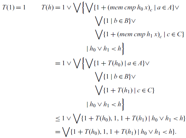
Again, we have essentially the same recurrence as given by the informal analysis. The last inequality is valid because A, B, and C are all subsets of  $\{*\}$, and hence are either $\emptyset$ or $\{*\}$ itself, and we take advantage of the fact that $\bigvee\!\emptyset = 0$. The comparison with $\infty$ might be a bit perturbing. In this model, the labels do not contribute to the potential of a tree. Since the comparison in the recurrence arises from the comparison of x with an arbitrary node label y, the best we can say about the potential of y is that it is at most $\infty$. For another perspective, keep in mind that cmp is monotone, so unless it is a particularly odd function, $cmp(x,\infty) = \{*\}\sqcup\{*\}\sqcup\{*\}$, which forces the recurrence to take all possible outcomes into account. This is precisely what we would expect in an informal analysis.
7.2.6 Inductive types as an abstract interpretation
Our justification for the interpretation of sum types appealed to intuition from abstract interpretation. For datatypes with structure functors that are sums of products (e.g., lists and trees), the connection goes beyond just intuition, as it is easy to see that not only do we have that  $\underline{\mathrm{D}}\mathbin\circ\underline{\mathrm{C}}\geq \mathop{\mathrm{id}}\nolimits$ $\beta_{\delta}$ but also that $\underline{\mathrm{C}}\mathbin\circ\underline{\mathrm{D}} = \mathop{\mathrm{id}}\nolimits$. This is precisely the kind of Galois connection we would expect to see in an abstract interpretation, where here we think of the datatype as being the abstract domain and its unfolding to be the concrete domain.Footnote 6
Intuitively, this is exactly how we think of models of the recurrence language as performing a size abstraction on datatypes. Interpreting a datatype value (i.e., an application of the constructor) as a size abstracts away information. Destructing a size tells us how a value of that size may be constructed from other data, but that data can only tell us the sizes of the substructures used in the construction. In other words, the application of the destructor gives us more concrete information about a size, namely, something about the composition of a value of that size.
$\underline{\mathrm{C}}\mathbin\circ\underline{\mathrm{D}} = \mathop{\mathrm{id}}\nolimits$. This is precisely the kind of Galois connection we would expect to see in an abstract interpretation, where here we think of the datatype as being the abstract domain and its unfolding to be the concrete domain.Footnote 6
Intuitively, this is exactly how we think of models of the recurrence language as performing a size abstraction on datatypes. Interpreting a datatype value (i.e., an application of the constructor) as a size abstracts away information. Destructing a size tells us how a value of that size may be constructed from other data, but that data can only tell us the sizes of the substructures used in the construction. In other words, the application of the destructor gives us more concrete information about a size, namely, something about the composition of a value of that size.
7.3 Counting all constructors
The cost of some functions cannot be usefully described in terms of the “usual” notion of size captured by the model  $\mathbf{V}$ of the previous section. For example, to usefully analyze the $\mathtt{sumtree}$ function of Figure 22, we need a model in which the size of a $\textsf{nat tree}$ value measures both the number of $\textsf{nat tree}$ constructors and the number of $\textsf{nat}$ constructors. In this section, we give an example of how to construct such a model. In it, a value v of inductive type is interpreted by a function $\phi$ such that $\phi(\delta)$ is the size of the largest maximal subtree of v that contains only $\delta$-constructors. For $v : \textsf{nat tree}$, this means that $[\![ v]\!] {}(\textsf{nat tree})$ is the usual size of v, $[\![ v]\!] {}(\textsf{nat})$ is the maximum label size of v, and $[\![ v]\!] {}(\delta) = 0$ for $\delta\notin\{\textsf{nat tree},\textsf{nat}\}$.
Because we want to distinguish between constructors for different inductive types, it is convenient to use the following alternative grammar for types and structure functors, which just spells out the closed-type production for structure functors:
 \[\begin{aligned}\sigma &::= \alpha \mid \textsf{C} \mid \textsf{unit} \mid \sigma+\sigma \mid \sigma\times\sigma \mid \sigma\to\sigma \mid \mu t F \\F &::= t \mid \alpha \mid \textsf{C} \mid \textsf{unit} \mid \mu t F \mid F + F \mid F \times F \mid \sigma \to F.\end{aligned}\tag{$*$}\]
The content of the next proposition is just that the grammar ( $*$) defines the same words as that of Figure 9.
1. If
$\sigma$ is a type by the grammar ($*$), then $\sigma$ is a structure functor by the grammar ($*$).-
2.
$\sigma$ is a type by the grammar of Figure 9 iff $\sigma$ is a type by the grammar ($*$), and F is a structure functor by the grammar of Figure 9 iff F is a structure functor by the grammar ($*$).


1. Induction on
$\sigma$.-
2. Induction on the
$\mu$-nesting depth of $\sigma$ and F. The main idea is that we treat t as a fixed symbol, rather than a meta-variable ranging over a class of variables, so inside the $\mu t.F$ production of F, it is no longer possible to refer to the “outer” t, and the $\mu t.F$ production of F always corresponds to a constant shape functor. ■


The type frame is the same as for the constructor-counting model of Section 7.2; for the current model, we write  $W^\sigma$ for the interpretation of $\sigma$. Except for inductive types, the clauses for $W^\sigma$ are the same as those for $V^\sigma$ from Section 7.2. Set $\mathcal D = \{\mu t F\}{\text{{F} closed}}$ and
•
$W^{\mu t F} = \{\phi \in D \to \mathbf{N}_0^\infty\} {\phi(\mu t F) \geq 1, \delta\text{not a syntactic subtype of F}\Rightarrow \phi(\delta) = 0}$.

To define  $\underline{\mathrm{C}}_{F}$ and $\underline{\mathrm{D}}_{F}$, we define $\underline{\mathrm{size}}_{F,\delta} : W^{F[\delta]}\to (\mathcal D\to\mathbf{N}_0^\infty)$ similarly to the previous section. The additional subscript enables us to track which datatype is the “main” datatype, as the counting is different for products for the main datatype and others. The definition is as follows:
 \[\begin{aligned}[t]\underline{\mathrm{size}}_{t,\delta}(\phi) &= \phi \\\underline{\mathrm{size}}_{\textsf{C},\delta}(x) &= {\lambda\hskip-.32em\lambda}\delta.0 \\\underline{\mathrm{size}}_{\textsf{unit},\delta}(*) &= {\lambda\hskip-.32em\lambda}\delta.0 \\\underline{\mathrm{size}}_{\mu t F,\delta}(\phi) &= \phi\end{aligned}\;\;\;\begin{aligned}[t]\!\!\!\!\underline{\mathrm{size}}_{{F_0}+{F_1},\delta}(X_0\sqcup X_1) &= \bigvee\underline{\mathrm{size}}_{F_0,\delta}[X_0] \vee \bigvee\underline{\mathrm{size}}_{F_1,\delta}[X_1] \\\underline{\mathrm{size}}_{{F_0}\times{F_1},\delta}(x_0, x_1) &= {\lambda\hskip-.32em\lambda}\delta'. \begin{cases} \underline{\mathrm{size}}_{F_0,\delta}(x_0)(\delta') + \underline{\mathrm{size}}_{F_1,\delta}(x_1)(\delta'), &\delta' = \delta \\ \underline{\mathrm{size}}_{F_0,\delta}(x_0)(\delta') \vee \underline{\mathrm{size}}_{F_1,\delta}(x_1)(\delta'), &\delta' \not= \delta \\ \end{cases} \\\underline{\mathrm{size}}_{\sigma\to F,\delta}(f) &= {\lambda\hskip-.32em\lambda}\delta'. \begin{cases} \sum\{\underline{\mathrm{size}}_{F,\delta}(f\,x)(\delta')\}{x\in D^\sigma}, &\delta' = \delta \\ \bigvee\{\underline{\mathrm{size}}_{F,\delta}(f\,x)(\delta')\}{x\in D^\sigma}, &\delta' \not= \delta \\ \end{cases}\end{aligned}\]
Set
 \[\underline{\mathrm{C}}_{F}(a) = {\lambda\hskip-.32em\lambda}\delta. \chi_F(\delta) + \underline{\mathrm{size}}_{F,\mu t F}(a)(\delta)\qquad\underline{\mathrm{D}}_{F}(\phi) = \bigvee\{a\}{\underline{\mathrm{C}}_{F}(a)\leq\phi}\]
where  $\chi_F(\delta) = 1$ if $\delta=\mu t F$, $\chi_F(\delta) = 0$ otherwise. Notice that for $\delta = \mu t F$, $\underline{\mathrm{C}}_{F}(a)(\delta) =1 + \underline{\mathrm{size}}_{F,\delta}(a)(\delta) \geq 1$, so $\underline{\mathrm{C}}_{F}(a)\in W^\delta$. $\textsf{fold}_\delta$ is interpreted by (std-fold) as usual.
7.3.1 Example: the potential of ${\textsf{nat tree}}$

Although we could prove a general theorem to show that  $\underline{\mathrm{size}}_{F,\delta}$ encapsulates the description given above, seeing the details of the specific case of $\textsf{nat tree}$ is more illuminating. To start, some notation is helpful: set $\phi^\textsf{nat}_n\in W^\textsf{nat}$ and $\phi^{\textsf{nat tree}}_{n,k}\in W^{\textsf{nat tree}}$ to be the functions
 \[\begin{aligned}[t]\phi^\textsf{nat}_n(\textsf{nat}) &= n \\\phi^\textsf{nat}_n(\underline{~}) &= 0\end{aligned}\qquad\begin{aligned}[t]\phi^{\textsf{nat tree}}_{n,k}(\textsf{nat}) &= n \\\phi^{\textsf{nat tree}}_{n,k}({\textsf{nat tree}}) &= k \\\phi^{\textsf{nat tree}}_{n,k}(\underline{~}) &= 0\end{aligned}\]
First we start with a useful lemma:
Lemma 9  $[\![ \textsf{S}]\!] {}(\phi) = \chi_{F_\textsf{nat}} + \phi$, and in particular, $[\![\textsf{S}]\!]{}(\phi^\textsf{nat}_k) = \phi^\textsf{nat}_{k+1}$.
 \begin{multline*}[\![{\textsf{S}}]\!]{}(\phi) = \chi_{F_\textsf{nat}} + \underline{\mathrm{size}}_{F_\textsf{nat},\textsf{nat}}(\underline{\mathrm{Inj}}^1(\phi)) = \chi_{F_\textsf{nat}} + \underline{\mathrm{size}}_{F_\textsf{nat},\textsf{nat}}(\emptyset\sqcup\downarrow\phi) = \\ \chi_{F_\textsf{nat}} + \left(\bigvee\underline{\mathrm{size}}_{t,\textsf{nat}}[\downarrow\phi]\right) = \chi_{F_\textsf{nat}} + \left(\bigvee(\downarrow\phi)\right) = \chi_{F_\textsf{nat}} + \phi.\end{multline*}
■
Now set  $\textsf{n} = \textsf{S}(\dotsc(\textsf{S}\,\textsf{Z})\dotsc) \mathbin:\textsf{nat}$ (n $\textsf{S}$s). We will show that $[\![{\textsf{n}}]\!]{} = \phi^\textsf{nat}_{n+1}$ by induction on n. For $n=0$,
 \begin{multline*}[\![{\textsf{0}}]\!]{} = \underline{\mathrm{C}}_{F_\textsf{nat}}(\underline{\mathrm{Inj}}^0 *) = \underline{\mathrm{C}}_{F_\textsf{nat}}(\{*\}\sqcup\emptyset) = \\ \chi_{F_\textsf{nat}} + \underline{\mathrm{size}}_{F_\textsf{nat},\textsf{nat}}(\{*\}\sqcup\emptyset) = \chi_{F_\textsf{nat}} + ({\lambda\hskip-.32em\lambda}\delta.0) = \chi_{F_\textsf{nat}} = \phi^\textsf{nat}_1.\end{multline*}
And for  $n\geq 0$, we use Lemma 9 to show that
 \[[\![{\textsf{n+1}}]\!]{} = ([\![{\textsf{S}}]\!]{}\,[\![{\textsf{n}}]\!]{}) = [\![{\textsf{S}}]\!]{}(\phi^\textsf{nat}_{n+1}) = \phi^\textsf{nat}_{n + 2}.\]
Now let us consider closed  $\textsf{nat tree}$ expressions built up using only $\textsf{nat tree}$ and $\textsf{nat}$ constructors—i.e., $\textsf{nat}$-labeled binary trees. We show that if t is such a tree, then $[\![{t}]\!]{} = \phi^{\textsf{nat tree}}_{m,k}$, where $m =\bigvee\{1+n\}{\text{{n} a label in {t}}}$ and k is the number of ${\textsf{nat tree}}$ constructors in t. In the following calculations, we will save a bit of space by writing $\underline{\mathrm{size}}_{F}$ for $\underline{\mathrm{size}}_{F,\textsf{nat tree}}$. For $\textsf{emp}$, the argument is essentially the same as for the analysis of $[\![{\textsf{0}}]\!]{}$, noting that $\bigvee\{1+n\mid\,n\,\text{a label in} \textsf{emp}\}=\bigvee\emptyset=0 $ For the inductive step, assume that $[\![{t_i}]\!]{} = \phi^{\textsf{nat tree}}_{n_i,k_i}$, so our goal is to show that $[\![{\textsf{node}(\textsf{n}, t_0, t_1)}]\!]{} =\phi^{\textsf{nat tree}}_{(n+1)\vee n_0\vee n_1,1+k_0+k_1}$:
 \begin{align*}[\![{\textsf{node}(\textsf{n}, t_0, t_1)}]\!]{} &= \underline{\mathrm{C}}_{F_{\textsf{nat tree}}}(\underline{\mathrm{Inj}}^1( [\![{\textsf{n}}]\!]{}, [\![{t_0}]\!]{}, [\![{t_1}]\!]{})) \\ &= \underline{\mathrm{C}}_{F_{\textsf{nat tree}}}( \emptyset\sqcup\downarrow(\phi^\textsf{nat}_{n+1}, \phi^{\textsf{nat tree}}_{n_0,k_0}, \phi^{\textsf{nat tree}}_{n_1,k_1})) \\ &= \chi_{F_{\textsf{nat tree}}} + \underline{\mathrm{size}}_{F_{\textsf{nat tree}}}( \emptyset\sqcup\downarrow(\phi^\textsf{nat}_{n+1}, \phi^{\textsf{nat tree}}_{n_0,k_0}, \phi^{\textsf{nat tree}}_{n_1,k_1})) \\ &= \chi_{F_{\textsf{nat tree}}} + \bigvee\underline{\mathrm{size}}_{\textsf{nat}\times{t\times t}}[ \downarrow(\phi^\textsf{nat}_{n+1}, \phi^{\textsf{nat tree}}_{n_0,k_0}, \phi^{\textsf{nat tree}}_{n_1,k_1}) ].\end{align*}
If  $(\phi',\phi_0',\phi_1')\in\downarrow(\phi^\textsf{nat}_{n+1}, \phi^{\textsf{nat tree}}_{n_0,k_0}, \phi^{\textsf{nat tree}}_{n_1,k_1})$, then
 \begin{align*}\underline{\mathrm{size}}_{{\textsf{nat}\times{t\times t}}}(\phi',\phi_0',\phi_1')(\delta) &= \begin{cases} \underline{\mathrm{size}}_{\textsf{nat}}(\phi')(\delta) + \underline{\mathrm{size}}_{t}(\phi_0')(\delta) + \underline{\mathrm{size}}_{t}(\phi_1')(\delta), &\delta={\textsf{nat tree}} \\ \underline{\mathrm{size}}_{\textsf{nat}}(\phi')(\delta) \vee \underline{\mathrm{size}}_{t}(\phi_0')(\delta) \vee \underline{\mathrm{size}}_{t}(\phi_1')(\delta), &\delta\not={\textsf{nat tree}} \end{cases} \\ &= \begin{cases} \phi'({\textsf{nat tree}}) + \phi_0'({\textsf{nat tree}}) + \phi_1'({\textsf{nat tree}}), &\delta = {\textsf{nat tree}} \\ \phi'(\delta) \vee \phi_0'(\delta) \vee \phi_1'(\delta), &\delta \not= {\textsf{nat tree}} \end{cases}\end{align*}
and hence the computation of  $[\![{\textsf{node}(\textsf{n}, t_0, t_1)}]\!]{}(\delta)$ proceeds as
 \begin{align*}{} &= \begin{cases} 1 + \bigvee \Biggl\{ \begin{aligned} &\phi'({\textsf{nat tree}}) + \phi_0'({\textsf{nat tree}}) + \phi_1'({\textsf{nat tree}})\mid \\ &\qquad{(\phi',\phi_0',\phi_1')\in\downarrow(\phi^\textsf{nat}_{n+1},\phi^{\textsf{nat tree}}_{n_0,k_0},\phi^{\textsf{nat tree}}_{n_1,k_1})} \end{aligned} \Biggr\}, &\delta = {\textsf{nat tree}} \\ \bigvee \Biggl\{ \begin{aligned} &\phi'(\delta) \vee \phi_0'(\delta) \vee \phi_1'(\delta)\mid \\ &{(\phi',\phi_0',\phi_1')\in\downarrow(\phi^\textsf{nat}_{n+1},\phi^{\textsf{nat tree}}_{n_0,k_0},\phi^{\textsf{nat tree}}_{n_1,k_1})} \end{aligned} \Biggr\}, &\delta \not= {\textsf{nat tree}} \end{cases} \\ &= \begin{cases} 1 + k_0 + k_1,&\delta = {\textsf{nat tree}} \\ (n+1) \vee n_0 \vee n_1,&\delta = \textsf{nat} \\ 0,&\text{otherwise} \end{cases} \\ &= \phi^{\textsf{nat tree}}_{(n+1)\vee n_0 \vee n_1, 1 + k_0 + k_1}(\delta).\end{align*}
We have simplified descriptions of recurrences that are analogous to those of Proposition 7:
1. If
$f\phi=[\![\mathsf{fold_{nat}}x \mathsf{of} \{\mathsf{Z}\Rightarrow e_Z|\mathsf{S}\Rightarrow r.e_{\mathsf{S}}\}]\!]\eta\{x\mapsto\phi\}$, then
\[f\,\phi^\mathsf{nat}_1 = [\![{e_\mathsf{Z}}]\!]\eta\qquad\begin{aligned}[t]f\,\phi^\mathsf{nat}_n &= [\![{e_\mathsf{Z}}]\!]\eta \vee \bigvee \{[\![ e_{\mathsf{S}}]\!] \eta\{r\mapsto\phi^{\mathsf{nat}}_{j}\}|j<n\} \\ &= [\![{e_\mathsf{Z}}]\!]\eta \vee [\![{e_\mathsf{S}}]\!] \eta\vee[\![ e_{\mathsf{S}}]\!] \eta\{r\mapsto\phi^{\mathsf{nat}}_{n-1}\} & & (n>1)\end{aligned}\]
-
2. If
$f\,\phi =[\![\mathsf{fold_{nat tree}}x \mathsf{of} \{\mathsf{emp}\Rightarrow e_{\mathsf{emp}}|\mathsf{node}\Rightarrow(x,r_0,r_1).e_{\mathsf{node}}\}]\!]\eta\{x\mapsto\phi\}$, then
\begin{align*}f\,\phi^{\mathsf{nat tree}}_{n,1} &= [\![{e_\mathsf{emp}}]\!]\eta \\f\,\phi^{\mathsf{nat tree}}_{n,k} &= [\![{e_\mathsf{emp}}]\!]{\eta} \vee \bigvee\!\! { [\![{e_\mathsf{node}}]\!] \eta{ \{x,r_0,r_1\mapsto \phi^\mathsf{nat}_{n'},f\,\phi^{{\mathsf{nat tree}}}_{n_0,k_0}, f\,\phi^{{\mathsf{nat tree}}}_{n_1,k_1}\}} } { n'\vee n_0\vee n_1\leq n, 1 + k_0 + k_1 \leq k } & & \!\!\!(n>1)\end{align*}


7.3.2 Example: summing the nodes of a $\mathtt{nat tree}$

Let us use this model to analyze the function  $\mathtt{sumtree} : \mathtt{nat tree}\rightarrow\mathtt{nat}$ that sums the nodes of a $\mathtt{nat tree}$. Its definition is given in Figure 22, along the relevant extracted recurrences. An informal analysis might proceed as follows. Because the cost of $\mathtt{sumtree}$ depends on both the cost and size of the result of $\mathtt{plus}$ as well as the size of the results of the recursive calls, we must extract recurrences for all of these. If $S_\mathtt{plus}(m, n)$ and $T_\mathtt{plus}(m, n)$ are the size of the result and the cost of $\mathtt{plus}(\underline{m-1}, \underline{n-1})$, respectively (recall from Figure 4 that $\underline{n}$ is the source language numeral for n), then an informal analysis yields the recurrences
 \[\begin{aligned}[t]S_\mathtt{plus}(1, n) &= n \\S_\mathtt{plus}(m, n) &= 1 + S_\mathtt{plus}(m-1, n)\end{aligned}\qquad\begin{aligned}[t]T_\mathtt{plus}(1, n) &= 1 \\T_\mathtt{plus}(m, n) &= 1 + T_\mathtt{plus}(m-1, n).\end{aligned}\]
Similarly, if  $S_\mathtt{st}(n, k)$ and $T_\mathtt{st}(n, k)$ are the size of the result and the cost of $\mathtt{sumtree}(t)$ when t has maximum label size n and size k, we end up with the recurrences
 \begin{align*}S_\mathtt{st}(n, 1) &= 1 \\S_\mathtt{st}(n, k) &= \bigvee \{S_\mathtt{plus}(n, S_\mathtt{plus}(S_\mathtt{st}(n, k_0), S_\mathtt{st}(n, k_1)))\} {k_0+k_1
< k}\end{align*}
\begin{align*}S_\mathtt{st}(n, 1) &= 1 \\S_\mathtt{st}(n, k) &= \bigvee \{S_\mathtt{plus}(n, S_\mathtt{plus}(S_\mathtt{st}(n, k_0), S_\mathtt{st}(n, k_1)))\} {k_0+k_1
< k}\end{align*}
and
 \begin{align*}T_\mathtt{st}(n, 1) &= 1 \\T_\mathtt{st}(n, k) &= \begin{aligned}[t] \bigvee \{ &T_\mathtt{st}(n, k_0) + T_\mathtt{st}(n, k_1) + T_\mathtt{plus}(S_\mathtt{st}(n, k_0), S_\mathtt{st}(n, k_1)) + \\ &\qquad T_\mathtt{plus}(n, S_\mathtt{plus}(S_\mathtt{st}(n, k_0), S_\mathtt{st}(n, k_1))) \mid k_0 + k_1
< k \}. \end{aligned}\end{align*}
\begin{align*}T_\mathtt{st}(n, 1) &= 1 \\T_\mathtt{st}(n, k) &= \begin{aligned}[t] \bigvee \{ &T_\mathtt{st}(n, k_0) + T_\mathtt{st}(n, k_1) + T_\mathtt{plus}(S_\mathtt{st}(n, k_0), S_\mathtt{st}(n, k_1)) + \\ &\qquad T_\mathtt{plus}(n, S_\mathtt{plus}(S_\mathtt{st}(n, k_0), S_\mathtt{st}(n, k_1))) \mid k_0 + k_1
< k \}. \end{aligned}\end{align*}
To solve these recurrences, one would first use any standard technique to conclude that  $S_\mathtt{plus}(m, n) = m+n-1$ and $T_\mathtt{plus}(m, n) = m$ to simplify the recurrence clauses for $S_\mathtt{st}$ and $T_\mathtt{st}$, then establish bounds on the latter by induction. However, the solution of the recurrences is not our focus here, but rather the justified extraction of them.
Now let us turn to our formal analysis. Set  $\tilde S_\textsf{plus}(\phi,\phi') = ([\![{\textsf{plus}}]\!]{}\,\phi\,\phi')_p$. Then making use of Proposition 9, $\tilde S_\textsf{plus}(\phi^\textsf{nat}_1,\phi') = \phi'$ and for $m>1$,
 \begin{align*}\tilde S_\textsf{plus}(\phi^\textsf{nat}_m,\phi') &= \phi' \vee [\![{\textsf{S}(r_p)}]\!] {\{r\mapsto {[\![{\textsf{plus}}]\!]{}\,\phi^\textsf{nat}_{m-1}\,\phi'}\}} \\ &= \phi' \vee (\chi_{F_\textsf{nat}} + {{[\![{\textsf{plus}}]\!]{}\,\phi^\textsf{nat}_{m-1}\,\phi'}}) & & \text{(Proposition 9)} \\ &= \phi' \vee (\chi_{F_\textsf{nat}} + \tilde S_\textsf{plus}(\phi^\textsf{nat}_{m-1},\phi'))\end{align*}
This recursive description of  $\tilde S_\textsf{plus}$ is sufficient to prove that $\tilde S_\textsf{plus}(\phi^\textsf{nat}_m,\phi') \geq \phi'$, and so we can conclude the reasoning with
 \[\tilde S_\textsf{plus}(\phi^\textsf{nat}_m,\phi') =\chi_{F_\textsf{nat}} + \tilde S_\textsf{plus}(\phi^\textsf{nat}_{m-1},\phi')\]
and so in particular
 \[\tilde S_\textsf{plus}(\phi^\textsf{nat}_1,\phi^\textsf{nat}_n) = \phi^\textsf{nat}_n\qquad\tilde S_\textsf{plus}(\phi^\textsf{nat}_m,\phi^\textsf{nat}_n) =\chi_{F_\textsf{nat}} + \tilde S_\textsf{plus}(\phi^\textsf{nat}_{m-1},\phi^\textsf{nat}_n),\]
recurrences that are equivalent to those derived informally. The analysis of  $\tilde T_\textsf{plus}(\phi,\phi') = ([\![{\textsf{plus}}]\!]{}\,\phi\,\phi')_c$ is similar and results in the recurrence
 \[\tilde T_\textsf{plus}(\phi^\textsf{nat}_1,\phi^\textsf{nat}_n) = 1\qquad\tilde T_\textsf{plus}(\phi^\textsf{nat}_m,\phi^\textsf{nat}_n) =1 + \tilde T_\textsf{plus}(\phi^\textsf{nat}_{m-1},\phi^\textsf{nat}_n).\]
Now set  $\tilde S_\textsf{st}(\phi) = ([\![{\textsf{sumtree}}]\!]{}\,\phi)_p$. Making use of Proposition 9, $\tilde S_\textsf{st}(\phi^{\textsf{nat tree}}_{1,k}) = \phi^\textsf{nat}_1$ and for $k>1$,
 \begin{align*}\tilde S_\mathsf{st}(\phi^{\mathsf{nat tree}}_{n,k}) &= \phi^\mathsf{nat}_1 \vee \bigvee \begin{aligned}[t] & \{([\![\mathsf{plus} x(\mathsf{plus r_{0_{p}}r_{1_{p}}})]\!]\{x,r_{i}\mapsto\phi^{\mathsf{nat}}_{n'},[\![\mathsf{suntree}]\!]\phi^{\mathsf{nat tree}}_{n_i,k_i}\})_p\\ & \qquad \mid n'\vee n_0 \vee n_1 \leq n, k_0+k_1 < k \bigr\} \end{aligned} \\ &= \phi^\mathsf{nat}_1 \vee \bigvee \begin{aligned}[t] & \bigl\{ ([\![{\mathsf{plus}}]\!]{}\,\phi^\mathsf{nat}_{n'}( [\![{\mathsf{plus}}]\!]{}\,(\tilde S_\mathsf{st}(\phi^{\mathsf{nat tree}}_{n_0,k_0}))\, (\tilde S_\mathsf{st}(\phi^{\mathsf{nat tree}}_{n_1,k_1})) )_{p})_{p} \\ & \qquad \mid n'\vee n_0 \vee n_1 \leq n, k_0+k_1 < k \bigr\} \end{aligned} \\ &= \phi^\mathsf{nat}_1 \vee \bigvee \begin{aligned}[t] & \bigl\{ \tilde S_\mathsf{plus}( \phi^\mathsf{nat}_{n'}, \tilde S_\mathsf{plus}( \tilde S_\mathsf{st}(\phi^{\mathsf{nat tree}}_{n_0,k_0}), \tilde S_\mathsf{st}(\phi^{\mathsf{nat tree}}_{n_1,k_1}) ) ) \\ & \qquad \mid n'\vee n_0 \vee n_1 \leq n, k_0+k_1
< k \bigr\} \end{aligned} \end{align*}
\begin{align*}\tilde S_\mathsf{st}(\phi^{\mathsf{nat tree}}_{n,k}) &= \phi^\mathsf{nat}_1 \vee \bigvee \begin{aligned}[t] & \{([\![\mathsf{plus} x(\mathsf{plus r_{0_{p}}r_{1_{p}}})]\!]\{x,r_{i}\mapsto\phi^{\mathsf{nat}}_{n'},[\![\mathsf{suntree}]\!]\phi^{\mathsf{nat tree}}_{n_i,k_i}\})_p\\ & \qquad \mid n'\vee n_0 \vee n_1 \leq n, k_0+k_1 < k \bigr\} \end{aligned} \\ &= \phi^\mathsf{nat}_1 \vee \bigvee \begin{aligned}[t] & \bigl\{ ([\![{\mathsf{plus}}]\!]{}\,\phi^\mathsf{nat}_{n'}( [\![{\mathsf{plus}}]\!]{}\,(\tilde S_\mathsf{st}(\phi^{\mathsf{nat tree}}_{n_0,k_0}))\, (\tilde S_\mathsf{st}(\phi^{\mathsf{nat tree}}_{n_1,k_1})) )_{p})_{p} \\ & \qquad \mid n'\vee n_0 \vee n_1 \leq n, k_0+k_1 < k \bigr\} \end{aligned} \\ &= \phi^\mathsf{nat}_1 \vee \bigvee \begin{aligned}[t] & \bigl\{ \tilde S_\mathsf{plus}( \phi^\mathsf{nat}_{n'}, \tilde S_\mathsf{plus}( \tilde S_\mathsf{st}(\phi^{\mathsf{nat tree}}_{n_0,k_0}), \tilde S_\mathsf{st}(\phi^{\mathsf{nat tree}}_{n_1,k_1}) ) ) \\ & \qquad \mid n'\vee n_0 \vee n_1 \leq n, k_0+k_1
< k \bigr\} \end{aligned} \end{align*}
Since  $\phi^\textsf{nat}_1$ is the bottom element of $W^\textsf{nat}$ and we can prove from this recurrence that $\tilde S_\textsf{st}(\phi^{\textsf{nat tree}}_{n,k})$ is monotone with respect to n, we can conclude this reasoning with
 \[\tilde S_\textsf{st}(\phi^{\textsf{nat tree}}_{n,k}) =\bigvee\{ \tilde S_\textsf{plus}( \phi^\textsf{nat}_{n}, \tilde S_\textsf{plus}( \tilde S_\textsf{st}(\phi^{\textsf{nat tree}}_{n,k_0}), \tilde S_\textsf{st}(\phi^{\textsf{nat tree}}_{n,k_1}) ) )\}{k_0+k_1
< k},\]
\[\tilde S_\textsf{st}(\phi^{\textsf{nat tree}}_{n,k}) =\bigvee\{ \tilde S_\textsf{plus}( \phi^\textsf{nat}_{n}, \tilde S_\textsf{plus}( \tilde S_\textsf{st}(\phi^{\textsf{nat tree}}_{n,k_0}), \tilde S_\textsf{st}(\phi^{\textsf{nat tree}}_{n,k_1}) ) )\}{k_0+k_1
< k},\]
which is analogous to the recurrence we derived informally. The analysis of  $\tilde T_\textsf{st}(\phi^{\textsf{nat tree}}_{n,k}) =([\![{\textsf{sumtree}}]\!]{}\,\phi^{\textsf{nat tree}}_{n,k})_c$ is similar and leads to

As a final note, in order to obtain the desired final form, we sometimes had to do some reasoning about the function on the basis of its recurrence, such as proving that the function is monotone. In fact, such reasoning is almost always required in the informal analysis as well, even though we typically gloss over such points when analyzing algorithms.
In may be helpful to contrast this analysis with the interpretation of  $\textsf{plus}$ and $\textsf{sumtree}$ in the model of Section 7.2. Since $\textsf{nat}$ values involve no other datatype constructors, the interpretation of $\textsf{plus}$ is essentially just the same, only requiring less notation to write down. However, the cost component of $[\![{\textsf{sumtree}}]\!]{\{n/ t\}}$ is less helpful. Because the model of Section 7.2 only accounts for the tree constructors, it does not account for the sizes of the node labels, and so this computation includes the cost component of $[\![{\textsf{plus}\,x\,({\textsf{plus}\,{r_{0_{p}}}\,{r_{1_{p}}}})_p}]\!] {{{\infty,\ldots/}{x,r_0, r_1}}}$ and this will result in a bound of $\infty$ (cf. to the occurrence of $\infty$ in the analysis of $\mathtt{mem}$ in the previous section, which did no harm there). This is correct as a bound. It reflects a cost analysis in which we have decided that we are counting each recursive call as a computation step, but then analyze a program in which data values whose size we ignore is the source of some recursive calls. However, this rather poor choice of size for this particular context yields a very weak bound, and so shows more generally that the choice of model does really matter.
7.4 Size abstraction and polymorphism: merging the constructor-counting models
Let us make a couple of observations about the previous two sections. It seems at least intuitive that counting only the main constructors is a more abstract notion of size than counting all constructors. And it also seems that even if we are working in the model of Section 7.3, if we have a polymorphic function in hand, it ought to be analyzable by just counting main constructors. This leads to the idea that if we have a model in hand (such as counting all constructors), then at least in some cases, it ought to be possible to interpret polymorphic recurrences so that the potentials arise from a more abstract notion of size than that given by the model. We give an example of how that might be done now.
Definition Suppose  ${\mathbf{U}} = (\mathbf{U}_{sm}, \mathbf{U}_{lg}, \{D^\sigma\})$ and ${\mathbf{U}}' = (\mathbf{U}_{sm}, \mathbf{U}_{lg},\{D'\}^\sigma)$ are two models of the recurrence language, both based on the (same extension of the) standard type frame. We say that ${\mathbf{U}}'$ is an abstraction of ${\mathbf{U}}$, or ${\mathbf{U}}$ is a concretization of ${\mathbf{U}}'$, if for every $\sigma\in\mathbf{U}_{sm}$ there are functions
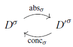
such that for all  $\sigma$, $\mathrm{conc}_\sigma$ is monotone, $\mathrm{conc}_\sigma\mathbin\circ\mathrm{abs}_\sigma\geq\mathop{\mathrm{id}}\nolimits_{D^\sigma}$ and $\mathrm{abs}_\sigma\mathbin\circ\mathrm{conc}_\sigma = \mathop{\mathrm{id}}\nolimits_{D'^\sigma}$.
Definition Suppose  ${\mathbf{U}}' = (\mathbf{U}_{sm}, \mathbf{U}_{lg}, \{D'\}^\sigma)$ is an abstraction of ${\mathbf{U}} = (\mathbf{U}_{sm}, \mathbf{U}_{lg}, \{D^\sigma\})$. The polymorphic abstraction of ${\mathbf{U}}$ relative to ${\mathbf{U}}'$ is the model ${\mathbf{U}}\to{\mathbf{U}}' = (\mathbf{U}_{sm}, \mathbf{U}_{lg}, \{B^\sigma\})$ that is defined as follows:
• For
$\sigma\in\mathbf{U}_{sm}$, $B^\sigma = D^\sigma$, with the semantic functions for small types taken from ${\mathbf{U}}$.-
• For
$\tau\in\mathbf{U}_{lg}\setminus\mathbf{U}_{sm}$, $B^\tau = {D'}^\tau$, where: -
• If
$\rho$ is quantifier-free and $\mathop{\mathrm{fv}}\nolimits(\rho)\subseteq\{\alpha\}$, then
-
• If
$\tau$ is not quantifier-free and $\mathop{\mathrm{fv}}\nolimits(\tau)\subseteq\{\alpha\}$, then we take $\underline{TyAbs}_{\lambda\hskip-.32em\lambda\sigma.\tau\{\sigma/\alpha\}} =\underline{TyAbs}_{\lambda\hskip-.32em\lambda\sigma.\tau\{\sigma/\alpha\}}^{{\mathbf{U}}'}$ and $\underline{TyAbs}_{\lambda\hskip-.32em\lambda\sigma.\tau\{\sigma/\alpha\}} =\underline{TyAbs}_{\lambda\hskip-.32em\lambda}\sigma.\tau\{\sigma/\alpha\}^{{\mathbf{U}}'}$.


1. If
${\mathbf{U}}$ and ${\mathbf{U}}'$ are applicative structures, then ${\mathbf{U}}\to{\mathbf{U}}'$ is an applicative structure.-
2. If
${\mathbf{U}}$ and ${\mathbf{U}}'$ are premodels such that whenever $\Gamma\vdash e:\rho$ and $\eta$ is a $\Gamma$-environment, ${\lambda\hskip-.32em\lambda}\sigma.[\![{\mathrm{abs}_{\rho\{\sigma/\alpha\}}(e)}]\!] \eta\{\alpha\mapsto\sigma\} \in\mathrm{Dom}\;\underline{TyAbs}^{{\mathbf{U}}'}$, then ${\mathbf{U}}\to{\mathbf{U}}'$ is a premodel.


Proof. The only nontrivial verification is that when  $\rho$ is quantifier-free and $\mathop{\mathrm{fv}}\nolimits(\rho)\subseteq\{\alpha\}$, $\underline{\mathrm{TyApp}}_{\lambda\hskip-.32em\lambda\sigma.\rho\{\sigma/\alpha\}}( \underline{TyAbs}_{\lambda\hskip-.32em\lambda\sigma.\rho\{\sigma/\alpha\}}\,f )\geq f$:
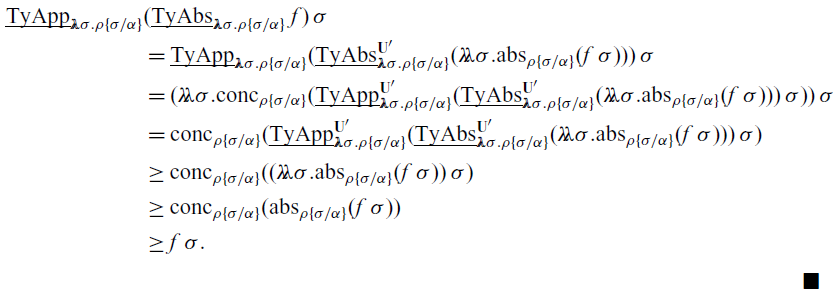
As an example, we define abstraction and concretization functions in Figure 23 that show that the main constructor counting model  $\mathbf{V}$ from Section 7.2 is an abstraction of the all-constructor counting model $\mathbf{W}$ from Section 7.3.

Fig. 23. Abstraction and concretization functions that relate the all-constructor (concrete) and main-constructor (abstract) models.
1.
$\mathrm{abs}_\sigma$ and $\mathrm{conc}_\sigma$ are monotone for all $\sigma$.-
2.
$\mathrm{abs}_\sigma\mathbin\circ\mathrm{conc}_\sigma = \mathop{\mathrm{id}}\nolimits$ and $\mathrm{conc}_\sigma\mathbin\circ\mathrm{abs}_\sigma \geq\mathop{\mathrm{id}}\nolimits$.


1. By induction on
$\sigma$.-
2. By induction on
$\sigma$; we just do $\sigma ={\sigma_0}+{\sigma_1}$. Let us write abs for $\mathrm{abs}_{{\sigma_0}+{\sigma_1}}$, $\mathrm{abs}_i$ for $\mathrm{abs}_{\sigma_i}$, and similarly for conc. To see that $\mathrm{abs}\mathbin\circ\mathrm{conc} = \mathop{\mathrm{id}}\nolimits$, notice that $(\mathrm{abs}\mathbin\circ\mathrm{conc})(Y_0\sqcup Y_1) =\downarrow\mathrm{abs}_0[\downarrow\mathrm{conc}_0[Y_0]]\sqcup\downarrow\mathrm{abs}_1[\downarrow\mathrm{conc}_1[Y_1]]$, so if $a'\in(\mathrm{abs}\mathbin\circ\mathrm{conc})(Y_0\sqcup Y_1)$, then there are i, b, and $a\in Y_i$ such that $a'\leq\mathrm{abs}_i(b)$ and $b\leq \mathrm{conc}_i(a)$, and hence $a'\leq\mathrm{abs}_i(\mathrm{conc}_i(a)) = a$ (by monotonicity and the induction hypothesis). But since $Y_i$ is downward closed, $a'\in Y_i$, so $(\mathrm{abs}\mathbin\circ\mathrm{conc})(Y_0\sqcup Y_1) \subseteq Y_0\sqcup Y_1$. To see that $\mathrm{abs}\mathbin\circ\mathrm{conc}\geq\mathop{\mathrm{id}}\nolimits$, notice that if $a\in Y_0\sqcup Y_1$, then $a\in Y_i$ for some i, and henc $a = \mathrm{abs}_i(\mathrm{conc}_i(a))\in\downarrow\mathrm{abs}_0[\downarrow\mathrm{conc}_0[Y_0]]\sqcup\downarrow\mathrm{abs}_1[\downarrow\mathrm{conc}_1[Y_1]] =(\mathrm{abs}\mathbin\circ\mathrm{conc})(Y_0\sqcup Y_1)$, so $Y_0\sqcup Y_1 \subseteq (\mathrm{abs}\mathbin\circ\mathrm{conc})(Y_0\sqcup Y_1)$.To see that $\mathrm{conc}\mathbin\circ\mathrm{abs}\geq\mathop{\mathrm{id}}\nolimits$, suppose $b\in X_i$. Then by the induction hypothesis $b\leq(\mathrm{conc}_i\mathbin\circ\mathrm{abs}_i)(b)$, and by unraveling the definition, $(\mathrm{conc}_i\mathbin\circ\mathrm{abs}_i)(b)\in\downarrow\mathrm{conc}_i[\downarrow\mathrm{abs}_i[X_i]]$. Since $\downarrow\mathrm{conc}_i[\downarrow\mathrm{abs}_i[X_i]]$ is downward closed, $b\in\downarrow\mathrm{conc}_i[\downarrow\mathrm{abs}_i[X_i]] \subseteq(\mathrm{conc}\mathbin\circ\mathrm{abs})(X_0\sqcup X_1)$.


Proposition 12  $\mathbf{W}\to\mathbf{V}$ is a model.

The definition of the abstraction and concretization functions in Figure 23 looks fairly canonical, so a natural question is whether for any two models of the recurrence language one can extend given functions on the interpretations of base types to all small types. In fact these definitions are an instance of a general pattern, but to state the pattern we will need a few definitions. A 2-category is a generalization of a category with a notion of morphism-between-morphism: if X and Y are objects, and  $f,g : X\longrightarrow Y$ are morphisms, then we will write $f\le_{\mathcal{C}} g : X \longrightarrow Y$ for a 2-cell from f to g. We will mainly consider the 2-category $\mathbf{Preorder}$, whose objects X,Y are preordered sets, whose morphisms $f : X\longrightarrow Y$ are monotone functions, and whose 2-cells $f \le g :X \longrightarrow Y$ are bounds $\forall x:X. f(x) \le_Y g(x)$. We will also need $\mathbf{Preorder}^{op}$ (the 1-cell dual of $\mathbf{Preorder}$): the objects are again preorders, a 1-cell $X\longrightarrow_{\mathbf{Preorder}^{op}} Y$ in $\mathbf{Preorder}^{op}$ is a 1-cell in $Y \longrightarrow_{\mathbf{Preorder}} X$, i.e. a monotone function $Y \to X$, but the 2-cells $f \le_{Preorder^{op}} g :X \longrightarrow_{Preorder^{op}} Y$ are still the 2-cells $f\le_{\mathbf{Preorder}} g : Y \longrightarrow_{\mathbf{Preorder}} X$, i.e. $\forall y:Y. f(y) \le_X g(y)$. A standard construction is to take the cartesian product of two 2-categories, where the objects, 1-cells, and 2-cells are given pointwise; in particular we will consider $\mathbf{Preorder} \times \mathbf{Preorder}$ and $\mathbf{Preorder}^{op}\times \mathbf{Preorder}$. A 2-functor $F : \mathcal{C} \to\mathcal{D}$ between 2-categories acts on objects, 1-cells (preserving identity and composition either strictly or up to 2-cell isomorphism), and 2-cells. For example, a (strict) 2-functor $F : \mathbf{Preorder}\to \mathbf{Preorder}$ consists of (0) for each preorder X, a preorder F(X); (1) for each monotone function $f : X \to Y$, a monotone function $F(f) : F(X) \to F(Y)$ such that $F(id) = id$ and $F(g \circ f)= F(g) \circ F(f)$; (2) if $\forall x:X. f(x) \le_Y g(x)$ then $\forall w:F(X). F(f) w \le_{F(Y)} F(g) w$. I.e. F sends preorders to preorders and monotone functions to monotone functions, in such a way that if g bounds f then F(g) bounds F(f).
An abstract interpretation in the sense above is often called a Galois insertion, which is a reflection in  $\mathbf{Preorder}$: a (strict) reflection of A into C consists of a pair of 1-cells $\mathrm{abs} \dashv \mathrm{conc}$ where $\mathrm{abs} : C \to A$ and $\mathrm{conc} : A \to C$, with an equality $\mathrm{abs} \circ \mathrm{conc} = id_A$ and a 2-cell $id_C \le_C \mathrm{conc} \circ \mathrm{abs}$. A standard observation is that any 2-functor $F : \mathcal{C} \to \mathcal{D}$ preserves reflections (this is used, for example, in domain theory Smyth & Plotkin Reference Smyth and Plotkin1982): if $\mathrm{abs} \dashv \mathrm{conc}$ is a reflection then $F(\mathrm{abs}) \dashv F(\mathrm{conc})$ is a reflection between F(C) and F(A). Applying F to the equality $\mathrm{abs} \circ \mathrm{conc} = id_A$ and using strict preservation of identity and composition gives $F(\mathrm{abs})\circ F(\mathrm{conc}) = id_{F(A)}$, and using the action on 2-cells of F on $id_C \le_C \mathrm{conc} \circ \mathrm{abs}$ (and again preservation of identity and composition) gives $id_{F(C)} \le_{F(C)} F(\mathrm{conc}) \circ F(\mathrm{abs})$.
This all means that we can lift the abstraction and concretization from base types to any type constructor that extends to a 2-functor. The product of preorders  $X \times Y$ is the action on objects of a functor $\mathbf{Preorder} \times \mathbf{Preorder} \to\mathbf{Preorder}$, where the action on maps $f_0 : X_0 \to X_0'$ and $g: X_1 \to X_1'$ is given by
 \[f_0 \times f_1 : X_0 \times X_1 \to X_0' \times X_1' := z \mapsto \langle f_0 (\pi_0 z), f_1(\pi_1 z) \rangle\]
This acts on 2-cells (preserves bounds) because pairing and application are monotone operations. To show that it preserves composition, we need a full  $\beta$-reduction equation and to show that it preserves identity, we also need the corresponding $\eta$/surjective pairing equation. However, these are true for the standard cartesian product of preorders. A reflection in $\mathbf{Preorder} \times \mathbf{Preorder}$ is a pair of reflections for each component. Unwinding these definitions gives the definitions of $\mathrm{abs}_{\sigma_0 \times \sigma_1}$ and $\mathrm{conc}_{\sigma_0 \times \sigma_1}$ in Figure 23.
The case of sums is more interesting. The standard coproduct of preorders  $X + Y$ is the disjoint union $X \sqcup Y$ ordered as defined above. This extends to a 2-functor $\mathbf{Preorder} \times\mathbf{Preorder} \to \mathbf{Preorder}$ with $f_0 + f_1$ defined via case-analysis. This is bound-preserving because the branches of a case-analysis (on the standard coproduct in preorders) are a monotone position and preserves identity/composition if we have $\beta\eta$ equations for case-analysis, which $X+Y$ does.
In the models under consideration, we do not define  $D^{\sigma_0+\sigma_1}$ to be $D^{\sigma_0} + D^{\sigma_1}$, but $\mathcal{O}{(D^{\sigma_0} + D^{\sigma_1})}$. However, it is also the case that $\mathcal{O}$ is a 2-functor $\mathbf{Preorder} \to\mathbf{Preorder}$: $\mathcal{O}{f} : \mathcal{O}{X} \to \mathcal{O}{Y}$ is $\downarrow \{ f(x) : x \in X \}$, which preserves bounds and identities and compositions. The composition of 2-functors is again a 2-functor, so $\mathcal{O}{(- + -)} : \mathbf{Preorder} \times \mathbf{Preorder} \to\mathbf{Preorder}$ is as well, and unwinding definitions gives $\mathrm{abs}_{\sigma_0+\sigma_1}$ and $\mathrm{conc}_{\sigma_0+\sigma_1}$ from Figure 23.
For functions, the preorder of pointwise-ordered monotone maps  $X \to Y$ extends to a mixed-variance 2-functor $\mathbf{Preorder}^{op} \times\mathbf{Preorder} \to \mathbf{Preorder}$, with functorial action given by pre- and post-composition. Moreover, a reflection $\mathrm{abs} \dashv\mathrm{conc}$ in $\mathbf{Preorder}$ is a reflection $\mathrm{conc} \dashv \mathrm{abs}$ in $\mathbf{Preorder}^{op}$ with the roles of concretization and abstraction exchanged. This unpacks to the definitions of $\mathrm{abs}_{\rho \to \sigma}$ and $\mathrm{conc}_{\rho \to \sigma}$ in Figure 23, where abstraction precomposes with concretization, and vice versa.
Thus, while our general definition of model does not require types to be interpreted as 2-functors—for example, being a model does not require the  $\eta$ law for pairs that ensures preservation of identities—a number of more specific models will have this form, and thus admit the same definition of relativized model, given abstraction and concretization for base/inductive types. For example, we may freely apply $\mathord{}$ in the interpretation of any type constructor, e.g., defining $D^{\sigma_0\times\sigma_1}$ to be $\mathcal{O}{(D^{\sigma_0} \times D^{\sigma_1})}$ for more precision.
7.4.1 Example: list reverse
To get a sense of how polymorphic abstraction behaves, let us analyze the polymorphic linear-time list reverse function given in Figure 24 in the model  $\mathbf{W}\to\mathbf{V}$. We choose this model because on the one hand $\mathbf{W}$ provides enough information for analyzing monomorphic functions like $\mathtt{sumtree}$ that depend on more than just the usual notion of size, yet we still want to analyze a polymorphic function like list reversal in terms of list length, ignoring any information about the elements of the argument list. Since polymorphism in the source language arises only via let-bindings, the recurrence for $\textsf{rev}'$ that is given is the recurrence that is substituted for for $\textsf{rev}'$ according to the definition of extraction for $\mathtt{let}$-expressions. A typical informal analysis of $\mathtt{rev}$ would really analyze $\mathtt{rev}'$ and might define S(n, m) and T(n, m) to be the size and cost of $\mathtt{rev}'\,xs\,ys$ when xs and ys have length n and m, respectively. One would then observe that S and T satisfy the recurrences
 \[\begin{aligned}[t]S(1, m) &= m \\S(n, m) &= S(n-1, m+1)\end{aligned}\qquad\begin{aligned}[t]T(1, m) &= 1 \\T(n, m) &= 1 + T(n-1, m)\end{aligned}\]
from which one establishes the O(n) bound on cost.

Fig. 24. Linear-time list reversal and its extracted recurrences.
Just as with our other models, to analyze  $\textsf{rev}$, we must consider its instantiation at some arbitrary small type $\sigma$. In the model $\mathbf{W}$, this would entail understanding how to compute $\underline{\mathrm{Fold}}^\mathbf{W}\,s\,\phi$ for arbitrary $\phi$, which would be defined in terms of all $\phi'\leq\phi$. The key point of $\mathbf{W}\to\mathbf{V}$ is that while we cannot avoid considering the instantiation of $\textsf{rev}$ at arbitrary $\sigma$, we only need to know how to compute $\underline{\mathrm{Fold}}^\mathbf{W}\,s\,\phi$ for those $\phi$ that are the concretizations of values in $V^{\sigma\textsf{list}}$. To see this, let us define $\phi^{\sigma\textsf{list}}_n = \mathrm{conc}_{\sigma\textsf{list}}(n)$—observe that $\phi^{\sigma\textsf{list}}_n$ maps $\sigma\textsf{list}$ to n and all other datatypes to $\infty$—and then compute $\textsf{rev}'$, where we write $f_\sigma\,\phi$ for $[\![\textsf{fold}_{\sigma\textsf{list}} xs \textsf{of} \{\textsf{nil}\Rightarrow\cdots|\textsf{cons}\Rightarrow\cdots\}]\!]\eta\{xs\mapsto\phi\}$:

When restricted to concretizations of abstract values,  $\underline{\mathrm{Fold}}^\mathbf{W}$ is straightforward to compute.
Proposition 13. If  $f\,n = [\![\textsf{fold}_{\sigma\textsf{list}}y \textsf{of}\{\textsf{nil}\Rightarrow e_{nil}|\textsf{cons}\Rightarrow(x,r).e_{\textsf{cons}}\}]\!]\eta\{y\mapsto\phi^{\sigma\textsf{list}}_{n}\}^{\mathbf{W}}$, then
 \begin{align*}f\,1 &= [\![{e_\textsf{nil}}]\!]\eta \\f\,n &= [\![{e_\textsf{nil}}]\!]\eta \vee [\![{e_\textsf{cons}}]\!] {\eta \{x, r\mapsto \infty^\sigma, f(n-1) \} } & & (n > 1).\end{align*}
With this in mind, set  $\tilde S(n, m) = \mathrm{abs}( (f_\sigma\,\phi^{\sigma\textsf{list}}_n )_p\,\phi^{\sigma\textsf{list}}_m)_p$. Our goal is to write a recurrence for $\tilde S(n, m)$. We start with
 \begin{align*}\tilde S(1, m) &= \mathrm{abs}((f_\sigma\,\phi^{\sigma\textsf{list}}_1)_p\,\phi^{\sigma\textsf{list}}_m)_p \\ &=\mathrm{abs}(([\![(1,\lambda zs.(0,zs))]\!])_p\phi^{\sigma\textsf{list}}_m)_p &= \mathrm{abs}({\lambda\hskip-.32em\lambda}\phi.(0, \phi)\,\phi^{\sigma\textsf{list}}_m)_p \\ &= \mathrm{abs}(0,\phi^{\sigma\textsf{list}}_m)_p \\ &= \mathrm{abs}(\phi^{\sigma\textsf{list}}_m) \\ &= m.\end{align*}
To compute  $\tilde S(n, m)$ for $n>1$, we first compute
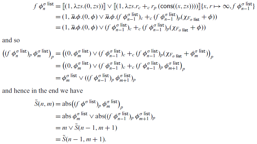
Analysis of cost proceeds in a similar manner. We have again extracted the recurrences we expect from an informal analysis, but instead of those recurrences being in terms of arbitrary values in  $W^{\sigma\textsf{list}}$, they are in terms of the length of the argument list.
Stepping back a bit, recall from Section 7.1 that we can apply parametricity to the standard model to reason about the cost of  $\mathtt{rev}\,xs$, which seems comparable to what we have just done. But there is a difference. The result from parametricity tells us that the cost of the result is determined by the length of the argument, but it does not tell us how to compute the former in terms of the latter. What we have done here is to formally justify the recurrence that does just that.
7.5 Lower bounds and an application to map fusion
So far, we have focused on extracting recurrences for upper bounds. However, the syntactic bounding theorem is agnostic with respect to the actual interpretation of the size order. We take advantage of this to derive recurrences for upper and lower bounds in the main constructor counting model of Section 7.2. Let us consider the  $\mathtt{map}$ function given in Figure 25. By reasoning that is by now hopefully somewhat mundane, if we set $T_{\mathtt{map}\,f}(n) = ([\![{\textsf{map}}]\!]{}\,f\,n)_c$, then we obtain the recurrence
 \[T_{\mathtt{map}\,f}(1) = 1\qquad T_{\mathtt{map}\,f}(n) = 1 + (f\,\infty)_c + T_{\mathtt{map}\,f}(n-1).\]
Solving this recurrence yields an upper bound of  $T_{\mathtt{map}\,f}(n) = n(1 + (f\,\infty)_c)$. Now let us apply this to the two sides of the usual map fusion law
 \[\mathtt{map}\,f\,(\mathtt{map}\,g\,xs) = \mathtt{map}\,(f\mathbin\circ g)\,xs.\]
We hope to show that the right-hand side is less costly than the left. Working through the recurrence extractions, we conclude that the cost of the left-hand side is bounded by  $T_{\mathtt{map}\,f\mathbin\circ\mathtt{map}\,g}(n) = 2n(1 + (g\,\infty)_c + (f\,\infty)_c)$, whereas the right-hand side is bounded by $T_{\mathtt{map}(f\mathbin\circ g)}(n) = n(1 + (g\,\infty)_c + (f(g\,\infty)_p)_c)$. Even under the assumption that the costs of f and g are independent of their arguments does not result in the desired conclusion, because we only know that these recurrences yield upper bounds, and the fact that one upper bound is larger than another tells us nothing about the actual costs. What we would like to know is that these recurrences are tight, and for that we need lower bounds as well.

Fig. 25. List map and its extracted recurrence.
As we already mentioned, as long as we have a model of the recurrence language in which the interpretation of the size order satisfies the axioms of Figure 11, the bounding theorem holds. So to obtain lower bounds, we would want a model in which the order on the interpretation of  $\textsf{C}$ is the reverse of the usual order. That means we would have two models in hand, one that gives us upper bounds and one that gives us lower bounds; we would then have to ensure that the recurrences in each model can be sensibly compared. As it turns out, we can arrange that by using the model in Section 7.2 because the interpretations of the types are all complete upper semi-lattices. We take advantage of the fact that a complete upper semi-lattice is in fact a complete lattice, where greatest lower bounds are defined by $\bigwedge X = \bigvee\{x\}{\forall y\in X: x\leq y}$. This permits us to define the dual interpretation of the model $(\mathbf{U}_{sm},\mathbf{U}_{lg},\{V^\sigma\}{\sigma})$ to be $(\mathbf{U}_{sm},\mathbf{U}_{lg},\{(V^*)^\sigma\}{\sigma})$, where $(V^*)^\sigma = (V^\sigma, \leq^*_\sigma)$ and $x\leq^*_\sigma y$ iff $y\leq_\sigma x$. Because all of the size-order axioms except $\beta_{\delta}$ and $\beta_{\delta\textsf{fold}}$ are witnessed by identities in $\mathbf{V}$ (i.e., the left- and right-hand sides of the axioms have the same denotation), we can take the semantic functions in $\mathbf{V}^*$ not related to datatypes to be those of $\mathbf{V}$. For datatype-related functions, it is unnecessary to change either $\underline{\mathrm{size}}_{F}$ or $\underline{\mathrm{C}}_{F}$; the only change needed is that we define
 \[\underline{\mathrm{D}}_{F}^*(n) = \bigwedge\{a\}{\underline{\mathrm{C}}_{F}(a)\geq n}.\]
We can verify that  $\beta_{\delta}$ holds by observing that
 \[\underline{\mathrm{D}}_{F}^*(\underline{\mathrm{C}}_{F}(a)) = \bigwedge\{a'\}{\underline{\mathrm{C}}_{F}(a')\geq \underline{\mathrm{C}}_{F}(a)} \leq a\]
and hence  $\underline{\mathrm{D}}_{F}^*(\underline{\mathrm{C}}_{F}(a)) \geq^* a$ as required. Of course, the value of the destructor is different in this model, but not by much; a routine calculation shows that
 \[\underline{\mathrm{D}}_{F_{\sigma\textsf{list}}}(x) = \emptyset\sqcup(\{\bot_\sigma\}\times\downarrow[\mathbf{N}_1^\infty](x-1));\]
compare this to the calculation in Section 7.2.
We likewise can define the semantic fold function in this model by
 \begin{align*}\underline{\mathrm{Fold}}_{F}^*\,s\,x &= \bigwedge\{s(\underline{\mathrm{Map}}(\underline{\mathrm{Fold}}\,s)\,z)\}{\underline{\mathrm{C}}_{F} z\geq x}\end{align*}
Similar to the computation of  $\underline{\mathrm{D}}_{F}$, we have an analogue of Proposition 7: if $f\,n = [\![\textsf{fold}_{\sigma\textsf{list}}y \textsf{of} \{\textsf{nil}\Rightarrow e_{\textsf{nil}}\mid\textsf{cons}\Rightarrow(x,r).e_{\textsf{cons}}\}]\!]\eta\{y\mapsto n\}$, then
 \begin{align*}f\,1 &= \bot_\sigma \\f\,n &= [\![{e_\textsf{cons}}]\!]\eta{\{x,r\mapsto\bot_\sigma,f(n-1)\}}.\end{align*}
Returning to our discussion of comparing the costs of  $\mathtt{map}\,f \mathbin\circ \mathtt{map}\,g$ and $\mathtt{map}({}f\mathbin\circ g)$, we now conclude that $T^\ell_{\mathtt{map}\,f\mathbin\circ\,\mathtt{map}\,g}(n) = 2n(1+(g\,\bot)_c + ({}f\,\bot)_c)$ is a lower bound on the cost of $\mathtt{map}\,f\mathbin\circ\mathtt{map}\,g$, so to show that $\mathtt{map}\,({}f\mathbin\circ g)$ is the more efficient alternative, it suffices to show that
 \[n(1 + (g\infty)_c + ({}f(g\,\infty)_p)_c)\leq_\textsf{C}2n(1+(g\,\bot)_c + ({}f\,\bot)_c),\]
which is trivial when the costs of f and g are independent of their arguments.
8 Recursion
We have not included general recursion in our languages in order to focus on the key idea that different models formally justify various informal cost analyses. The presence of recursion does not change this perspective, but it does complicate the model descriptions in ways orthogonal to our main thrust. We sketch the approach of Kavvos et al. (Reference Kavvos, Morehouse, Licata and Danner2020) here.
For the syntax, we add recursive definitions to the source language with a standard  $\mathtt{letrec}$ construct and to the recurrence language with a standard $\textsf{fix}$ constructor, corresponding to the usual approach for call-by-value and call-by-name languages. The details are given in Figure 26, where we also give two new size-order rules to replace $\beta_{\delta\textsf{fold}}$. In these new rules, $\mathcal E$ is an elimination context and $\textsf{fix}_{n}\,{x}.{e}$ is defined by
 \[\textsf{fix}_{0}\,{x}.{e} = \textsf{fix}\,{x}.{x}\qquad\textsf{fix}_{n+1}\,{x}.{e} = e \{\textsf{fix}_{n}\,{x}.{e}\}/{x}.\]
The two rules codify the relation between the size order and the information order that is implicit in the presence of  $\textsf{fix}$: a more defined bound is a better (i.e., smaller) bound. In the presence of nontermination, the bounding relation requires a slight adjustment: $e\preceq E$ provided: if E terminates, then ${e\theta}\downarrow^{n}{v}$, where $n\leq E_c$ and $v\preceq^{val} {E_p}$. This is the only place a (standard) operational semantics is needed in the recurrence language, and we are investigating how to eliminate its use.

Fig. 26. Adding general recursion to the source and recurrence languages.
For the semantics of the recurrence language, we impose additional structure on our applicative structures. We call the new structures sized domains and they are defined just like applicative structures, except that for each  $U\in\mathbf{U}_{sm}$, $D^U = (D^U,\leq_U,\sqsubseteq_U, \bot_U)$, where $(D^U,\leq_U)$ is a preorder as before, and $(D^U,\sqsubseteq_U,\bot_U)$ is a complete partial order. The semantic domains must satisfy two additional constraints:
• If
$x\sqsubseteq_U y$, then $y\leq_U x$; and-
• If
$y_0\sqsubseteq_U y_1\sqsubseteq_U\dotsb$ and for all i, $x\leq_U y_i$, then $x\leq\bigsqcup y_i$.


That leaves us with verifying that the models that we presented in Section 7 are sized domains. For each of the models, we take  $\sqsubseteq_{\mathbf{N}_i^\infty}$ to be the usual flat order with $\bot_{\mathbf{N}_i^\infty} = \infty$ (again, cf. Rosendahl Reference Rosendahl1989) extended pointwise and componentwise for functions and products. For sums, set $X\sqsubseteq Y$ if $Y\subseteq X$. It is a straightforward exercise to show that $D^{\rho+\sigma}$ is a CPO that satisfies the constraints just given. To show that we have a model, it suffices to verify that the semantic functions are simultaneously monotone with respect to $\leq$ and continuous with respect to $\sqsubseteq$, after which Proposition 6 can be extended with the clause that ${\lambda\hskip-.32em\lambda} a.[\![{\Gamma\vdash e: \sigma}]\!]\eta\{x\mapsto a\}$ is continuous with respect to $\sqsubseteq$. Verification of continuity for $\underline{\mathrm{CASE}}$ relies on two facts that hold in these models at all types:
• If
$a\sqsubseteq a'$ and $b\sqsubseteq b'$, then $(a\vee b)\sqsubseteq(a'\vee b')$; and-
• If
$a_0\sqsubseteq a_1\dotsb$ and $b_0\sqsubseteq b_1\dotsb$, then $\bigsqcup\{a_i\vee b_i\} = (\bigsqcup a_i)\vee(\bigsqcup b_i)$.


Extracting syntactic recurrences from general recursive functions and interpreting them in our models follows the same pattern we have already seen several times. But now the recurrences may have more complex solutions (such as poly-log solutions). For example, Kavvos et al. (Reference Kavvos, Morehouse, Licata and Danner2020) analyze the standard implementation of merge-sort and interpret it in the model of Section 7.2. Under the usual assumption that the cost of the comparison function is constant the recurrence clause of the semantic recurrence is  $T(n) = c + dn + T(n/2)$ for some constants c and d (that arise from the analyses of the functions that divide a list in two and merge two sorted lists), just as expected. Now one may reason in the semantics to establish the $O(n\lg n)$ cost from this recurrence.
Quick-sort provides an interesting example of how more complex models can be used to capture subtle information that may be necessary for an asymptotic analysis. Quick-sort relies on a partitioning function  $\mathtt{part} :\alpha\rightarrow\alpha\textsf{list}\rightarrow\alpha\textsf{list}\times\alpha\textsf{list}$ such that $\mathtt{part}\,x\,xs = (ys, zs)$, where ys consists of the elements of xs that are $< x$ and zs those elements that are $\geq x$. A key part of the analysis of quick-sort is the fact that the sum of the lengths of ys and zs is the length of xs. In the models we have presented in Section 7, the extracted recurrence will not yield such a bound. For example, in the main constructor-counting model, the best we can conclude about the extracted recurrence is that in the semantics, $\textsf{part}\,x\,n = (n,n)$. The problem is that the interpretation of products requires that we choose some specific pair that is a bound on all pairs $(k,\ell)$ such that $k+\ell = n$, and (n, n) is the least such bound. But we have seen this situation before when it came to interpreting sums, and the solution is the same: instead of taking $V^{\rho\times\sigma} = V^{\rho}\times V^{\sigma}$, we can instead take $V^{\rho\times\sigma} = \mathcal{O}(V^\rho\times V^\sigma)$. While the calculations become more tedious, in such a model we can show that $\textsf{part}\,x\,n = \{(k,\ell)\}{k+\ell \leq n}$. However, it turns out this is not quite enough. Both the source and recurrence languages have negative products, which means that projections must be used to extract ys and zs. In the interpretation of the extracted recurrence, projection of a set of pairs maximizes over the corresponding component, and so $\pi_i {(\textsf{part}\,x\,n)} = n$ (because $n+0 = 0 + n = n$), which again leads to a weak bound. Instead, we must use positive products with an elimination of the form $\mathtt{split}\,(x, y) = e^{\rho\times\sigma}\,\mathtt{in}\,e'$. The corresponding elimination form in the recurrence language can be interpreted by maximizing $[\![{e'}]\!]{}$ over all pairs in $[\![{e}]\!]{}$, which is precisely what is needed to carry out the rest of the usual analysis of quick-sort.
9 Related work
We first expand upon a couple of observations that we made earlier and mention some motivating history behind some technical details. Then we address how our work fits into the literature on cost analysis.
We touched on an application of parametricity in Section 7.1. Seidel & VoigtlÄnder (Reference Seidel and VoigtlÄnder2011) have interpreted free theorems (Wadler Reference Wadler1989) to obtain relative complexity information. Their work can be viewed as applying parametricity to the standard model, but in a somewhat more general setting of a recurrence language that has a monadic type constructor  $\textsf{C}(\sigma)$ for “complexity of $\sigma$,” with projections for cost and potential. They define a notion of lifting relations to complexities (much as relations are lifted to inductive types), which allows them to interpret a free theorem such as $f(\mathtt{hd}\,xs) = \mathtt{hd}(\mathtt{map}\,f\,xs)$ in such a way that the interpretations of both sides yield complexity information, and the identity then allows them to conclude, e.g., that the cost of the left-hand side is no greater than that of the right-hand side. With our approach, we would simply extract recurrences from the left- and right-hand sides and reason about them as in Section 7.5. While on the topic of relative cost information, we would be remiss to not mention the type-and-effect system of ÇiÇek et al. (Reference ÇiÇek, Barthe, Gaboardi, Garg and Hoffmann2017), which permits a very precise analysis of the relative cost of different algorithms on the same arguments or the same algorithm on different arguments. We have not investigated whether our techniques can be adapted to provide comparable analyses.
We drew an analogy with abstract interpretation (AI) in Section 7.2.6 and made use of the existence of a Galois connection of the sort that arises in AI in Section 7.4. Rosendahl (Reference Rosendahl1989) uses AI to extract cost bounds directly from a first-order fragment of Lisp. She first defines a program translation similar to our syntactic extraction and interprets it in the standard model D of S-expressions. She then defines an AI from  ${{\mathcal P}(D)}$ into a finite-height lattice of “partial structures,” whose values are essentially truncated standard values. Given a notion of size $s : D\to\mathbf{N}$ and a computable bound on ${\lambda\hskip-.32em\lambda} n.\alpha(\{x\}{s(x)= n})$, the interpretation of the syntactic recurrence in the abstract domain is a computable upper bound on the cost of the original program. This work is restricted to first-order programs and does not handle branching data structures well (e.g., if s(t) is the number of nodes in the tree t, then for $n>1$, $\alpha(\{x\}{s(x) = n})$ is a node structure that is truncated at its children, so the bounds are all trivial). But these ideas may provide an approach to computing bounds on semantic recurrences in models where the semantic recurrence itself is not computable (a situation that does not arise in the models we have presented).
While our notion of potential is drawn most directly from Danner & Royer (Reference Danner and Royer2007), it traces back at least to Shultis (Reference Shultis1985), who defines a denotational semantics for a simple higher order language that models both the value and the cost of an expression. He develops a system of “tolls,” which play a role similar to that of our potentials. The tolls and the semantics are not used directly in calculations, but rather as components in a logic for reasoning about them. Sands (Reference Sands1990) defines a translation scheme in which each identifier f in the source language is associated to a cost closure that incorporates information about the value f takes on its arguments, the cost of applying f to arguments, and arity. Cost closures record information about the future cost of a partially applied function, just as our potentials do. The idea of using denotational semantics to captures cost information has been seen before. We have already mentioned Rosendahl (Reference Rosendahl1989) and Shultis (Reference Shultis1985). Van Stone (Reference Van Stone2003) defines a category-theoretic denotational semantics that uses “cost structures” (these include the  $\textsf{C} \times -$ writer monads we use here) to capture cost information and shows that it is sound with respect to a cost-annotated operational semantics for a higher order language. Our bounding theorem is roughly analogous to Van Stone’s soundness theorem, but is a bit more general because we show an inequality (using the size order on the complexity language) instead of an equality, which allows the bounding theorem to apply to models with size abstraction.
Turning now to the literature on cost analysis, constructing resource bounds from source code has a long history in Programming Languages. The earliest work known to the authors is that of Cohen & Zuckerman (Reference Cohen and Zuckerman1974), which extracts programs that describe costs from an ALGOL60-like language that are intended to be manipulated in an interactive system, and Wegbreit’s (1975) METRIC system, which extracts recurrences from simple first-order recursive Lisp programs. An interesting aspect of the latter system is that it is possible to describe probability distributions on the input domain (e.g., the probability that the head of an input list will be some specified value), and the generated bounds incorporate this information. Le MÉtayer’s (1988) ACE system converts FP programs (Backus Reference Backus1978) (under a strict operational semantics) to FP programs (under a nonstrict semantics) describing the number of recursive calls of the source program. The first phase is comparable to the cost projection of our recurrence extraction; the potential projection is the original program. Both METRIC and ACE yield nonrecursive upper bounds on the generated cost functions (this is the bulk of the work for ACE). These systems are restricted in their datatypes and compute costs in terms of syntactic values; the notion of “size” is somewhat ad hoc and second class. Many approaches to cost analysis rely on the idea that the cost can be treated as an additional output of the program, or as a piece of program state; Wadler (Reference Wadler1992) observed that this can be represented by a monadic translation—though in our case we use the writer monad rather than the state monad, since we do not give programs access to their cost.
There are many approaches to type-based cost analysis (Crary & Weirich, Reference Crary and Weirich2000; Hofmann & Jost, Reference Hofmann and Jost2003; Jost et al., Reference Jost, Hammond, Loidl and Hofmann2010; Hoffmann & Hofmann, Reference Hoffmann and Hofmann2010; Hoffmann et al., Reference Hoffmann, Aehlig and Hofmann2012, Reference Hoffmann, Das and Weng2017; Jost et al., Reference Jost, Vasconcelos, Florido and Hammond2017; Knoth et al., Reference Knoth, Wang, Polikarpova and Hoffmann2019, Reference Knoth, Wang, Reynolds, Hoffmann and Polikarpova2020; Avanzini & Dal Lago, Reference Avanzini and Dal Lago2017; ÇiÇek et al., Reference ÇiÇek, Barthe, Gaboardi, Garg and Hoffmann2017; Wang et al., Reference Wang, Wang and Chlipala2017; Dal Lago & Gaboardi, Reference Dal Lago and Gaboardi2011; Handley et al., Reference Handley, Vazou and Hutton2019; Rajani et al., Reference Rajani, Gaboardi, Garg and Hoffmann2021). At a high level, these systems include special-purpose judgments or types that track cost, indexed or refinement types that track the size of values, and a type checking or inference mechanism that can automatically determine some resource bounds. For example, the Automatic Amortized Resource Analysis (AARA) technique of Hoffmann et al. (Reference Hoffmann, Aehlig and Hofmann2012), Hoffmann et al. (Reference Hoffmann, Das and Weng2017), Jost et al. (Reference Jost, Vasconcelos, Florido and Hammond2017), Hofmann & Jost (Reference Hofmann and Jost2003), Jost et al. (Reference Jost, Hammond, Loidl and Hofmann2010), Hoffmann & Hofmann (Reference Hoffmann and Hofmann2010), with an implementation at Hoffmann (Reference Hoffmann2020), computes cost bounds by introducing a type system with size information that is parameterized by an integer degree, and then performing type inference. If inference is successful, then the program cost can be bounded by a polynomial of at most that degree (and a bound is reported); otherwise it cannot). As its name suggests, AARA automatically incorporates amortization, resulting in tighter bounds for some programs than our extracted recurrences yield (but see Cutler et al. Reference Cutler, Licata and Danner2020 for an extension of our approach to amortized analysis). The basic AARA technique has been extended in numerous ways, e.g., with refinement types (Knoth et al. 2019; Reference Knoth, Wang, Reynolds, Hoffmann and Polikarpova2020) for synthesizing programs with desired resource bounds, and for more precise tracking of potential in values. The Timed ML system of Wang et al. (Reference Wang, Wang and Chlipala2017) also uses refinement types (indexed types in the style of DML Xi & Pfenning Reference Xi and Pfenning1999) that permit the user to define datatypes with their own notion of size and to include cost information in the program type. Type inference produces verification conditions that, if solvable, validate the cost information. That cost information may be very concrete, or left more open-ended, in which case the verification conditions end up synthesizing (recurrence) relations that must be satisfied. Avanzini & Dal Lago (Reference Avanzini and Dal Lago2017) develop a nonamortized type-based analysis, which uses a translation similar to our recurrence extraction to explicitly represent the cost as a unary numeral. As a result, the evaluation cost of the original program is reflected in the size of the cost component of the translated program. They then make use of an extension of sized types (Hughes et al. Reference Hughes, Pareto and Sabry1996) to infer a type for the translated program, which therefore includes a bound on the cost in terms of the size of the arguments.
All of these type-based approaches are impressive in the breadth of successful analyses and/or automation thereof. However, we believe it is nonetheless worth studying cost analysis by recurrence extraction for several reasons. First, the process of inferring bounds using these specialized type systems and their associated solvers is not, in our opinion, very easy for a person to do, while our focus is on formalizing the method that we readily teach students to do. Second, automated approaches necessarily impose some limits on the kinds of bounds that can be inferred and the notions of size that are supported to facilitate inference (though Handley et al. Reference Handley, Vazou and Hutton2019 also allows explicit proofs; see the discussion of techniques in proof assistants below). For example, AARA infers polynomial bounds, while our approach (adapted to the setting of general recursion) can produce recurrences with nonpolynomial solutions. Third, type-based approaches make the size and cost an intrinsic feature of the code: in approaches based on refinement types, one must, for example, define one tree type where size means number of nodes, and a different tree type where size means height, which causes code duplication if both are necessary; in amortized approaches, one must choose the potential annotations when defining a type (though sometimes this can be mitigated by parametrizing the datatypes Knoth et al. Reference Knoth, Wang, Reynolds, Hoffmann and Polikarpova2020). In our approach, cost and size are an extrinisic property of the code, so the same function can be interpreted in different models with different notions of size for different analyses, which can be useful, e.g., for a library function that is used in two different programs by other functions that require two different notions of size. That said, this does not address situations where two different notions of size for a type are needed in a single program—one possible solution is a model in which the potential is the pair of these sizes, but this would have similar reuse problems to changing a refinement type to include additional information, in that all existing analyses would formally need to be modified.
Let us now consider work that, like ours, externalizes cost from programs that are typed in a more-or-less standard type system. Avanzini et al. (Reference Avanzini, Dal Lago and Moser2015) carefully defunctionalize higher order programs to first-order programs in order to take advantage of existing techniques from first-order rewrite systems. This leverages existing technologies to great effect, but does not match the kind of recurrence extraction that we are aiming for in this work. The COSTA project (Albert et al. Reference Albert, Arenas, Genaim, Puebla and Zanardini2012) extracts cost recurrences from Java bytecode; Albert et al. (Reference Albert, Genaim and Masud2013) provide techniques for constructing closed forms for both lower and upper bounds on these recurrences. This group has also pushed forward on parallel cost (Albert et al. Reference Albert, Correas, Johnsen, Pun and RomÁn-Dez2018), something that Raymond (Reference Raymond2016) has looked into in our setting, but the COSTA work has focused on first-order, low-level languages.
Cutler et al. (Reference Cutler, Licata and Danner2020) adapt our technique to handle amortized analysis. Reinforcing our goal of formalizing informal approaches, the source language there includes constructions for describing a credit allocation policy (the banker’s method) and extraction of an amortized cost recurrence, to which a general theorem applies that total amortized cost bounds total actual cost. The language is sufficient for describing structures like splay trees in which the number of credits allocated to different parts of the structure is not constant, and the source language type system ensures that credits are not misused. The key point is that the amortized cost recurrence is extracted into essentially the same recurrence language as we have presented here, reflecting the fact that the recurrences that we use to describe amortized cost do not themselves refer to credits.
Kavvos et al. (Reference Kavvos, Morehouse, Licata and Danner2020) give an approach to extending our technique to handle general (as opposed to structural) recursion by using call-by-push-value (CBPV) (Levy Reference Levy2003) as an intermediate source language into which both call-by-value and call-by-name can be embedded. While CBPV includes a fine stratification of types into computational and value types, analyzing a program still really just relies on notions of size and cost. Thus, the syntactic recurrence language differs from the one just described only in replacing primitive recursion with a general fixpoint operator, along with corresponding axioms for the size order, thereby changing it from a version of System T with inductive types to a version of PCF with inductive types.
Atkey (Reference Atkey2011), GuÉneau et al. (Reference GuÉneau, CharguÉraud and Pottier2018), CharguÉraud & Pottier (Reference CharguÉraud and Pottier2019), and Zhan & Haslbeck (Reference Zhan and Haslbeck2018) develop imperative program logics for reasoning about cost based on separation logic, essentially by treating the number of timesteps taken as part of the heap. A Coq or Isabelle implementation of these logics allows for reasoning about code, and the subgoals that arise during verification result in synthesizing recurrence relations, which play the role of our syntactic recurrences. While quite sophisticated algorithms and data structures can be analyzed this way, including imperative ones, for analyzing functional programs, we find it more congruous to use (and teach to students) standard functional program verification techniques like inductive reasoning about outputs, as opposed to imperative program verification techniques like weakest precondition/characteristic formula generation. And as we note in Section 10, we conjecture that our approach extends to the analysis of many imperative programs because the description of cost itself is frequently a functional description.
Turning now to semi-automated/manual reasoning in a functional style, Danielsson (Reference Danielsson2008) verifies a number of lazy functional programs in Agda using a dependent type tracking the number of steps a program takes. McCarthy et al. (Reference McCarthy, Fetscher, New, Feltey and Findler2018) investigate a variant, implemented in Coq, using a monad parametrized by both the number of steps and a specification, given as a relation between the cost and value. The specifications are used both for functional correctness and for reasoning about cost, and this design allows Coq’s extraction to OCaml to erase all costs and reasoning about them. The library also provides a source-to-source translation that translates simply typed code into the monad, inserting appropriate ticks, which is analogous to our recurrence extraction. RadiČek et al. (Reference RadiČek, Barthe, Gaboardi, Garg and Zuleger2017) define a specification logic for reasoning about monadic costs as an extension of higher order logic.
Benzinger’s (2004) ACA system might be the closest in philosophy to ours, in that it extracts (higher order) recurrences from call-by-name NuPrl programs that bound the cost of those programs. There we find (moderately complex) expressions that correspond to applying higher order functions to arguments (necessarily alternating with projections) to describe the cost of a fully applied function argument, corresponding to our notion of higher-order potential. But this does not address more realistic call-by-value or call-by-need evaluation.
Since these approaches (Benzinger Reference Benzinger2004; Danielsson Reference Danielsson2008; RadiČek et al. Reference RadiČek, Barthe, Gaboardi, Garg and Zuleger2017; McCarthy et al. Reference McCarthy, Fetscher, New, Feltey and Findler2018) take place inside of a general-purpose logic or proof assistant, one can express costs in terms of the sizes of inputs by explicitly referring to an appropriate size function and proving how operations transform the size. Relative to this, a main contribution of our approach is to systematize and partially automate the reasoning about size, in the sense that our semantic interpretation of the potential of a function f gives a direct inductive definition of the fused “size of the result of f on inputs of size –” function. This is possible because we step outside of the programming language into a denotational setting where, e.g., arbitrary maximums exist. We claim that this corresponds better to informal analyses than using the full power of a proof assistant to carefully prove how functions act on sizes, because the fused size-to-size function will simplify in ways that the original function does not. For example, because in these models most or all contexts are monotone in the size order, one can freely ignore branches whose size is dominated by another.
10 Conclusions and further work
We have presented a technique for extracting cost-and-size recurrences from higher order functional programs that provably bound the operational cost in terms of user-definable notions of size, thereby giving a formal account of the process of many informal cost analyses. The technique applies to the pure fragment of strict languages such as ML and OCaml. Although we have not investigated the question carefully, it also seems that it applies to much reasoning about imperative programs. The reason is that such analysis often consists of extracting functional cost recurrences whose validity only depends on the fact that certain imperative operations have certain costs. For example, the analysis of many functions on an arrays depends on the fact that indexed access and update is constant time. But the analysis does not typically result in a recurrence that even refers to an array, much less destructively updates one. In our setting, we would either hard-code the costs of access and update in the syntactic recurrence extraction or we would leave those functions as identifiers and analyze the semantic recurrence under the assumption that those identifiers are interpreted by constant-time functions. The de facto standard for such reasoning is Separation Logic, and the work that ours seems closest to in spirit is that of Zhan & Haslbeck (Reference Zhan and Haslbeck2018). Our goal would be to provide relatively simple approaches to formalizing reasoning about many imperative programs. This is certainly speculative, and we have not investigated how far one can push this idea before requiring the machinery of something comparable to Separation Logic.
A natural direction to extend our work would be to handle cost analysis of lazy languages. Okasaki (Reference Okasaki1998) describes a technique of amortized analysis in which costs are split into “shared” and “unshared” costs in order to correctly account for the memoization of computations, and we believe our approach can be adapted to formalize this technique. Hackett & Hutton (Reference Hackett and Hutton2019) show that lazy evaluation is a form of “clairvoyant” call-by-value and that cost can be described nondeterministically rather than in terms of shared and unshared costs. We hope to adapt our approach to yield corresponding recurrences, especially as they actually compute costs via an interpretation in a denotational model that appears to mesh nicely with our approach.
We have presented several models making use of different notions of size. It is no surprise that it is easier to work in models with simpler notions of size, and we saw in Section 7.4 that a simpler notion of size corresponds to a more abstract model. Formalizing the connection between more abstract and more concrete models so that information from the latter may be pulled into the former would improve the usefulness of this sort of reasoning. This sounds like an analogy with safety and liveness theorems from abstract interpretation, and this is probably a fruitful direction for further study. More complex models should enable more sophisticated analysis. For example, the average case complexity of deterministic quick-sort can be described by assuming a (uniform) probability distribution on the inputs. That would seem to correspond to interpreting the usually extracted recurrence in a model in which inductive types are interpreted by probability distributions or random variables. Barnaby (Reference Barnaby2018) has made preliminary progress in this direction, which indicates that it is probably necessary to have at least limited forms of dependent typing in the recurrence language.
We have focused on the extraction of semantic recurrences to show that they are the ones that are expected from informal analysis. We have not studied techniques for solving the semantic recurrences, which in general are higher order functions. Benzinger (Reference Benzinger2004) discusses techniques for solving them by reducing them to first-order recurrence equations and then using off-the-shelf solvers such as Mathematica and OCRS (Kincaid et al. Reference Kincaid, Cyphert, Breck and Reps2017). Another fruitful direction would be to formalize the extracted semantic recurrences in proof assistants and make use of the formalization of standard theorems like the Master Theorem and of asymptotic reasoning as in GuÉneau et al. (Reference GuÉneau, CharguÉraud and Pottier2018). This would permit a formal development in a setting where complete automation is not possible.
The extraction of the syntactic recurrence is straightforward to implement, and a future project is to produce an end-to-end tool from source code to semantic recurrence to solution. We know that automated cost analysis is a complex project that many have attempted, and so this goal as stated is probably too ambitious, and we warn the reader that our thoughts here are pies in the sky at the time of writing. Our vision is more along the lines of an interactive system, in which recurrences are extracted and “easy” ones solved, but allowing the user to step in to provide assertions (hopefully proved!) about the solutions to difficult ones. Familiarity with recurrence extraction as a cost analysis technique would hopefully lower the entry barrier of such a tool. We could also hope that that same familiarity would enable users to work backward from an unexpectedly poor recurrence to the code from which it results (cf. Benzinger Reference Benzinger2004). Wang & Hoffmann (Reference Wang and Hoffmann2019) adapt AARA to provide worst-case inputs that validate the tightness of the produced bounds, which could be used to similar effect. Another direction such a project could take would be to pull either the syntactic or the semantic information back as additional interface-level components of a language library, so as to modularize cost reasoning and take advantage of the compositionality of our approach. However, this is not so straightforward. One issue that arises is that the denotation a type that is appropriate for analyzing an algorithm is not necessarily the one that is appropriate for using it. For example, the recurrence extraction approach works best to analyze binary search tree algorithms in terms of their heights, but a client who uses a binary search tree implementation is probably more interested in understanding the cost in terms of the size. This is a setting in which composing recurrences does not work as smoothly as we might hope. Understanding how to mesh them together, and more generally how to hide analyses that possibly require more complex types (such as those by Cutler et al. Reference Cutler, Licata and Danner2020) behind an interface, is ongoing work.
Acknowledgments
Both authors were supported by the National Science Foundation under grant number CCF 1618203. We had a number of helpful discussions about this work with colleagues, including Ed Morehouse, Alex Kavvos, and Joe Cutler. We thank the referees for a number of helpful comments and pointers to literature with which we were initially unfamiliar.
Conflicts of interest
None.
Type preservation for the source language
Type preservation depends on the usual substitution lemmas.
Lemma 10 If  ${\Gamma,x\mathbin:\rho}\vdash{e{(\theta-x)}}: \sigma$ and $_\vdash v \rho$, then $\Gamma\vdash {e\theta \{x\mapsto v\}}: \sigma$.
Lemma 11 If  ${y\mathbin:\rho}\vdash{v'}:{\sigma}$ and $_\vdash v\rho$, then ${v'}\{v/y\}$ is a value and $\vdash{{v'}\{v/y\}}:{\sigma}$.
We now have the type preservation theorem.
Theorem (Type preservation, Theorem 1)
If
$\_\vdash {e\theta}:{\sigma}$ and ${e\theta}\downarrow{v}$, then $\vdash v: \sigma$.If
$\_\vdash{{\mathtt{map}_F y.{v''} \mathtt{into} {v'}}{\theta}}: {F[\sigma]}$ and $\mathtt{map}_F y.v''\mathtt{into}v'\downarrow v$, then $\vdash v: {F[{\sigma}]}$.If
$\_\vdash{\mathtt{mapv}_F y.{v''} \mathtt{into} {v'}}: {F[{\sigma}]}$ and $\mathtt{mapv}_F y.v''\mathtt{into}v'\downarrow v$, then $\vdash v: {F[{\sigma}]}$.


Proof. The proof is a simultaneous induction on the height of the derivation that referred to in each part. We give just a few of the more interesting cases, starting with part (1). $\underline{\mathrm{CASE}:x\theta\downarrow\theta(x)}$ By the hypothesis, $\_\vdash {x\theta}:{\sigma}$, so by the typing rules for closures, there must be some $\Gamma'$ such that $\Gamma'(x) = \forall{\vec{\alpha}}.{\rho}$ and $\sigma = \rho\{\vec{\sigma}/\vec{\alpha}\}$, and $\theta$ is a $\Gamma'$-environment. But that means that in particular, $\vdash{\theta(x)}:{\rho{\vec{\sigma}}/{\vec{\alpha}}}$, as required. $\underline{(\mathtt{case}e \mathtt{of} \{x.e_{i}\}_{i=0,1})\theta\downarrow v}$ The typing must have the form
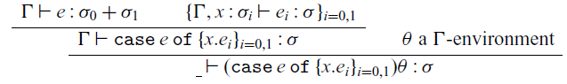
and the evaluation must have the form
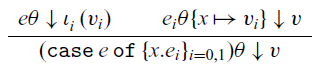
By definition  $\_\vdash{e\theta}:{{\sigma_0}+{\sigma_1}}$, so by the induction hypothesis, $_\vdash{\iota_i {v_i}}:{{\sigma_0}+{\sigma_1}}$, and hence by inversion, $_\vdash{v_i}{\sigma_i}$. That means that $\theta{x}\mapsto{v_i}$ is a $(\Gamma,x\mathbin:\sigma_i)$-environment, and hence $\_\vdash{{e_i}\theta\{{x}\mapsto{v_i}\}}:{\sigma}$. So by the induction hypothesis, $_\vdash v \sigma$, as required. ${(\lambda x.e)\theta}\downarrow{(\lambda x.e\theta)}$ If $\_\vdash({\lambda x.e\theta}):{{\sigma}\rightarrow{\sigma'}}$, then we must show that $\_\vdash ({\lambda x.e\theta}):{{\sigma}\rightarrow{\sigma'}}$ as a value. For this we must show that $\_\vdash ({\lambda x.e\theta}) {{\sigma}\rightarrow{\sigma'}}$ as a closure, which is precisely the hypothesis we started with. $({e_0}{e_1})\theta\downarrow{v}$ The typing has the form

and the evaluation has the form

Since  $\theta$ is a $\Gamma$-environment, $\_\vdash{{e_0}{\theta}}:{\rho\rightarrow\sigma}$, so by the induction hypothesis, $\vdash{(\lambda x.{e_0'}){\theta_0'}}:{\rho\rightarrow\sigma}$ and similarly $_\vdash{v_1}{\rho}$. By definition we have that there is some $\Gamma'$ such that ${\Gamma'}\vdash{\lambda x.{e_0'}}:{\rho\rightarrow\sigma}$ and $\theta_0'$ is a $\Gamma'$-environment; by inversion we have that ${\Gamma',x\mathbin:\rho}\vdash{e_0'}:{\sigma}$. Since $_\vdash{v_1}:{\rho}$, ${\theta_0'}\{x\mapsto v_1\}$ is a $(\Gamma',x\mathbin:\rho)$-environment, and so $\_\vdash{{e_0}{{\theta_0'}\{x\mapsto v_1\}}}:{\sigma}$, and so by the induction hypothesis, $\vdash v: \sigma$, as required. $\underline{\mathrm{CASE:}(\textsf{fold}_\delta e' \textsf{of} x.e)\theta\downarrow v}$ The typing must have the form

and the evaluation must have the form

where without loss of generality we assume  $y\notin\mathrm{Dom}\;\Gamma$ and $y\notin\mathrm{Dom}\;\theta$. By the assumptions and induction hypothesis, $\vdash{\textsf{c}_\delta {v'}}:{\delta}$, and so by inversion, $\vdash{v'}:{F[\delta]}$. From ${\Gamma,x\mathbin:F [\sigma\textsf{susp}]\vdash}{e}:{\sigma}$, we conclude that ${\Gamma,y\mathbin:\delta}\vdash\textsf{delay}(\textsf{fold}_\delta y \textsf{of} x.e):\sigma\textsf{susp}$. Since $\theta$ is a $\Gamma$-environment, we conclude that ${y\mathbin:\delta}\vdash(\textsf{delay}(\textsf{fold}_\delta y \textsf{of} x.e))\theta:\sigma\mathtt{susp}$. These two judgments allow us to conclude that $\_\vdash\textsf{mapv}_F y.(\textsf{delay}(\textsf{fold}_\delta y \textsf{of} x.e))\theta \textsf{into}v':F[\sigma\mathtt{susp}]$, so by the induction hypothesis applied to the evaluation of the $\mathtt{mapv}$ expression, $_\vdash{v''}:{F[\sigma\textsf{susp}]}$. That means that $\theta\{x\mapsto{v''}\}$ is a $(\Gamma,x\mathbin:F[\sigma\textsf{susp}])$-environment, and so by the induction hypothesis applied to the evaluation of $e\theta\{x\mapsto v''\}$, $\vdash{v}:{\sigma}$, as required.
For (2), suppose  $(\textsf{map}_F y.v' \textsf{into} e)\theta\downarrow v$. The typing must have the form

and the evaluation the form

As in previous cases,  $\vdash{v''}:{F[\rho]}$, and so $\_\vdash{\textsf{mapv}_F y.{v'} \textsf{into} {v''}}:{F[\sigma]}$, and so the result follows from the induction hypothesis applied to this $\mathtt{mapv}$ expression.
We now prove (3). $\underline{\mathrm{CASE}:\textsf{mapv}_t y.v'\textsf{into} v\downarrow v'\{v/y\}}$ From the typing assumption, we have that ${y\mathbin:\rho}\vdash{v'}:{\sigma}$ and $\vdash v: \rho$, so the result follows from Lemma 11. $\underline{\mathrm{CASE}:\textsf{mapv}_{\rho\rightarrow F}y.v'\textsf{into} (\lambda x.e)\theta\downarrow(\lambda x.\textsf{map}_F y.v' \textsf{into} e)\theta}$ The typing must have the form

Thus, we obtain a typing of the value as

Typeability of extracted recurrences
In this appendix we prove that extracted recurrences are typeable. It is worth remembering that  $\langle\langle{\rho\rightarrow\sigma}\rangle\rangle ={\langle\langle\rho\rangle\rangle}\rightarrow{\|\sigma\|}$, so extraction “commutes” with type substitution in the expected way.
Lemma 12  $\langle\langle\{\rho{\vec{\sigma}}{\vec{\alpha}}\}\rangle\rangle ={\langle\langle\rho\rangle\rangle}\{{\langle\langle\vec{\sigma}\rangle\rangle}\}/{\vec{\alpha}}$. Since shape functors are a subset of types, this implies that $\langle\langle{F\{\vec{\sigma}/\vec{\alpha}\}}\rangle\rangle ={\langle\langle{F}\rangle\rangle}\{\langle\langle\vec{\sigma}\rangle\rangle/\vec{\alpha}\}$ and $\langle\langle{F[\rho]}\rangle\rangle = {\langle\langle{F}\rangle\rangle}[{\langle\langle\rho\rangle\rangle}]$
Lemma 13 If  ${\Gamma, x\mathbin:\tau'}\vdash{e}:{\tau}$ and ${\Gamma}\vdash{e'}:{\tau'}$, then $\Gamma\vdash e\{e'/x\}:{\tau}$.
Lemma 14 If  $\Gamma\vdash{c}:{\textsf{C}}$ and $\Gamma\vdash e:{\|\sigma\|}$, then $\Gamma\vdash{c+_{c}{e}}:{\|\sigma\|}$.
Proposition (Typeability of extracted recurrences, Prop. 1) If  $\Gamma \vdash e : \tau$ is in the core language, then ${\langle\langle{\Gamma}\rangle\rangle}\vdash{\|e\|}:{\|\sigma\|}$.
Proof. The proof is by induction on the derivation of  $\Gamma \vdash e : \tau$; we just do a few of the cases, since they are all fairly routine. $\underline{\mathrm{CASE}:\Gamma,x:\forall\vec{\alpha}.\rho\vdash x:\rho\{\vec{\sigma}/\vec{alpha}\}}$ $\|x\| = (0,x)$ and $\|\rho\{\vec{\sigma}/\vec{\alpha}\}\|=\textsf{C}\times\langle\langle\rho\{\vec{\sigma}/\vec{\alpha}\}\rangle\rangle=\textsf{C}\times\langle\langle\rho\rangle\rangle\{\langle\langle\vec{\sigma}\rangle\rangle/\vec{\alpha}\}$; the recurrence language typing is
 $\underline{\mathrm{CASE:}\Gamma\vdash\lambda x.e:\rho\rightarrow\sigma}$ $\|{\rho\rightarrow\sigma}\| = \textsf{C}\times({\langle\langle\rho\rangle\rangle}\rightarrow{\|\sigma\|})$ and we have ${\Gamma,x\mathbin:\rho}\vdash{e}:{\sigma}$, so by the induction hypothesis, ${\langle\langle{\Gamma}\rangle\rangle,x\mathbin:\langle\langle\rho\rangle\rangle}\vdash {\|e\|}: {\|\sigma\|}$ and hence
 $\Gamma\vdash{\textsf{fold}_\delta {e'} \textsf{of} x.{e}}:{\sigma}$ The typing derivation has the form

so by the induction hypothesis  ${\langle\langle{\Gamma}\rangle\rangle}\vdash {\|e'\|}: {\textsf{C}\times{\langle\langle{\delta}\rangle\rangle}}$ and ${\langle\langle{\Gamma}\rangle\rangle,x\mathbin:{{\langle\langle{F}\rangle\rangle}[\|\sigma\|}]} {\|e\|}: {\|\sigma\|}$. Writing (c’, p’) for $\|e'\|$, by inversion we have that ${\langle\langle{\Gamma}\rangle\rangle}\vdash{c'}:{\textsf{C}}$ and ${\langle\langle{\Gamma}\rangle\rangle}\vdash{p'}:{\langle\langle\delta\rangle\rangle}$. We must show that $\langle\langle\Gamma\rangle\rangle\vdash c'+_c \textsf{fold}_{\langle\langle\delta\rangle\rangle}p' \textsf{of}(x:\langle\langle F\rangle\rangle[\|\sigma\|]).1+_c\|e\|:\|\sigma\|$. This follows directly from the typings given by the induction hypothesis, making use of the fact that $\langle\langle{F\{\eta\}}\rangle\rangle ={\langle\langle{F}\rangle\rangle}\{\langle\langle\vec{\sigma}\rangle\rangle\}/{\vec{\alpha}}$ and Lemma 14. $\underline{\mathrm{CASE:}\Gamma\vdash\textsf{let} x=e' \textsf{in} e:\sigma}$ The typing derivation has the form

The induction hypothesis tells us that  ${\langle\langle{\Gamma}\rangle\rangle}\vdash{\|e'\|}:{\|\rho\|}$, so if $\|e\|' = (c',p')$, then ${\langle\langle{\Gamma}\rangle\rangle}\vdash{c'}:{\textsf{C}}$ and ${\langle\langle{\Gamma}\rangle\rangle}\vdash{p'}:{\langle\langle\rho\rangle\rangle}$. From the latter we conclude that ${\langle\langle{\Gamma}\rangle\rangle}\vdash {\Lambda{\vec{\alpha}}.{p'}}: {\forall{\vec{\alpha}}.{\langle\langle\rho\rangle\rangle}}$ because $\vec{\alpha}\notin\mathrm{ftv}(\Gamma)$ implies that $\vec{\alpha}\notin\mathrm{ftv}(\langle\langle{\Gamma}\rangle\rangle)$. The induction hypothesis also tells us that ${\langle\langle{\Gamma}\rangle\rangle,x\mathbin:\forall{\vec{\alpha}}.{\langle\langle\rho\rangle\rangle}}\vdash {\|e\|}: {\|\sigma\|}$. Together with Lemma 13 we conclude that ${\langle\langle{\Gamma}\rangle\rangle}\vdash {\|e\|}\{\Lambda{\vec{\alpha}}.{p'}/{x}\} {\|\sigma\|}$ and so Lemma 14 yields the desired conclusion. ■
The syntactic bounding theorem
In this appendix, we prove the syntactic bounding theorem (Theorem 5). The proof relies on two lemmas that describe bounding for  $\mathtt{mapv}$ and $\mathtt{fold}$ expressions.
Lemma 15 (Syntactic bounding for  $\mathtt{mapv}$) Suppose $\mathrm{ftv}(F)\subseteq\{t\}$ and that the following all hold:
- ${y\mathbin:\rho}\vdash{v'}:\sigma$ and ${y\mathbin:\langle\langle\rho\rangle\rangle}\vdash{E'}:{\langle\langle\sigma\rangle\rangle}$.
- $\_\vdash{v}:{{F}[\rho]}$ and $\mathcal{E}:: {v\preceq^{\mathrm{val}}_F[\rho] E}$;
If
$\_\vdash{w_0}::{\rho}$ and ${\mathcal{E}_0}::{w_0\preceq^{\mathrm{val}}_\rho} E_0$ is a subderivation of $\mathcal{E}$ then ${{v'} \{w_0/y\}}{\preceq^{\mathrm{val}}_{\sigma}{E'} \{E_0}/y\}$;- $\mathtt{mapv}_F y.v' \textsf{into}v\downarrow v''$.


Then  $v''\preceq^{\mathrm{val}}_F[\sigma](\langle\langle F\rangle\rangle)[(y:\langle\langle\rho\rangle\rangle).E',E]$
Proof. The proof is by induction on F. $\underline{\mathrm{CASE:}F=t}$ Assumption (4) tells us that $v'' = {v'} \{v/y\}$, so we must show that $v'\{v/y\}\preceq^{\mathrm{val}}_{\sigma}E'\{E/y\}$, which follows from assumption (3), taking $v_0$ and $E_0$ to be v and E, respectively. $\underline{\mathrm{CASE:}F=\tau_0}$ Assumption (4) tells us that $v'' = v$, so we must show that ${v}\preceq^{\mathrm{val}}_{\tau_{0}}{E}$, which follows from assumption (2). $\underline{\mathrm{CASE:}F=F_0\times F_1}$ Assumption (2) and inversion tells us that $v = (V_0,V_1)$, and assumption (4) tells us that $v'' = ({v_0'',v_1''})$, where

We must show that  $(v^{''}_{0},v^{''}_{1})\preceq^{\mathrm{val}}(\langle\langle F_0\rangle\rangle[(y:\langle\langle\rho\rangle\rangle).E',\pi_0 E],\langle\langle F_1\rangle\rangle[(y:\langle\langle\rho\rangle\rangle).E',\pi_1 E])$, for which it suffices to show that ${v_i''}\preceq^{\mathrm{val}}\langle\langle F_i\rangle\rangle[(y:\langle\langle\rho\rangle\rangle).E',\pi_i E]$ for $i=0,1$. To do so, we apply the induction hypothesis taking $F_i$ for F, $v_i$ for v, $\pi_{i} E$ for E, and $v_i''$ for v”. Verifying the assumptions is straightforward, noting that (3) follows because the derivation that ${v_i}\preceq^{\mathrm{val}}{\pi_i E}$ is a subderivation of $(v_0,v_1)\preceq^{\mathrm{val}} E$. $\underline{\mathrm{CASE:}F=F_0+F_1}$ Assumption (2) and inversion tells us that $v = \iota_i {v_i}$, where there is $E_i$ such that ${v_i}\preceq^{\mathrm{val}}{E_i}$ and $\iota_i {E_i} \leq_{{\langle\langle{F_i}\rangle\rangle}[\rho]} E$. Assumption (4) tells us that $v'' = \iota_i {v_i''}$, where

We must show that
 \[\iota_{i}v^{''}_{i} \preceq^{\mathrm{Val}} \textsf{case} E \textsf{of} \{(x:\langle\langle F_i\rangle\rangle[\langle\langle\rho\rangle\rangle]).\iota_{i}\langle\langle F_i\rangle\rangle[(y:\langle\langle\rho\rangle\rangle).E',x]\}_{i=0,1}\]
Let us write  $E^*$ for the right-hand side. Now we must show that there is $E_i''$ such that ${v_i''}\preceq^{\mathrm{Val}}{E_i''}$ and $\iota_i{E_i''}\leq E^*$. We apply the induction hypothesis taking $F_i$ for F, $v_i$ for v, $E_i$ for E, and $v_i''$ for v” to conclude that ${v_i''}\preceq^{\mathrm{Val}}{E_i''}$ where $E_i'' = {\langle\langle{F_i}\rangle\rangle}[(y:\langle\langle\rho\rangle\rangle).{E'},{E_i}]$, and we notice that

as required. The assumptions for the induction hypothesis are straightforward to verify, noting that (3) follows because the derivation that  ${v_i}\preceq^{\mathrm{Val}}{E_i}$ is a subderivation of ${\iota_i {v_i}}\preceq^{\mathrm{Val}}{E}$. $\underline{\mathrm{CASE:}F=\iota_0\rightarrow F_0}$ Assumption (2) and inversion tells us that $v = {\lambda x.e}\theta$, and assumption (4) tells us that $v'' = {\lambda x.{\mathtt{map}_F y.{v'} \mathtt{into} e}}\theta$. We must show that

To do so, fix  ${v_1}\preceq^{\mathrm{Val}}_{\tau_0}{E_1}$; it suffices to show that $(\mathtt{map}_F y.v' \mathtt{into} e)\theta\{x\mapsto v_1\}\preceq_{F[\rho]}((E\,E_1)_{c},\langle\langle F\rangle\rangle[(y:\langle\langle\rho\rangle\rangle).E',(E E_1)_p]) $. The evaluation of the left-hand side has the form

so by Lemma 4 it suffices to show that  $n\leq {(E {E_1})_c}$ and $w\preceq^{\mathrm{Val}}{{\langle\langle{F}\rangle\rangle}[(y:\langle\langle\rho\rangle\rangle).E',(E E_1)_p]}$. Recalling that $v = {\lambda x.e}\theta$ and ${v}\preceq^{\mathrm{Val}}{E}$ by assumption (2), we have that $e\theta\{x\mapsto v_1\}\preceq E E_1$, and hence $n\leq {(E {E_1})}$ (our first obligation) and ${w'}\preceq^{\mathrm{Val}}{(E {E_1})_p}$. To show that $w\preceq^{\mathrm{Val}}{{\langle\langle{F}\rangle\rangle}[(y:\langle\langle\rho\rangle\rangle).E',(E E_1)_p]}$ we apply the induction hypothesis taking $F_0$ for F, w’ for v, $(E E_1)_p$ for E, and w for v”. Assumptions (1), (2), and (4) are straightforward to verify. For assumption (3), suppose that $\_\vdash{w_0}:{\rho}$ and ${\mathcal{E}_0}::{{w_0}\preceq^{\mathrm{Val}}{E_0}}$ is a subderivation of ${\mathcal{E'}}::{{w'}\preceq^{\mathrm{Val}}(E\,E_1)_p}$. We need to show that ${v'}\{w_0/y\}\preceq^{\mathrm{Val}}{{E'}\{E_0/y\}}$. To do so, it suffices to show that $\mathcal{E}_0$ is a subderivation of $\mathcal{E}::{{v}\preceq^{\mathrm{Val}}{E}}$, and for this it suffices to show that $\mathcal{E}'$ is a subderivation of $\mathcal{E}$. This follows from examining $\mathcal{E}$:

Lemma 16 (Syntactic bounding for  $\mathtt{fold}$) Suppose the following all hold:
- $(\Gamma,x:F[\sigma \mathtt{susp}]\vdash e:\sigma)\preceq_{\sigma}(\langle\langle\Gamma\rangle\rangle,x:\langle\langle{F}[\sigma \mathtt{susp}]\rangle\rangle\vdash E: \|\sigma\|$;
- $\theta\preceq^{\mathrm{Val}}_{\Gamma-x}\Theta$ (w.l.o.g., $x\notin\mathrm{Dom}\;\Theta$);
- ${v'}\preceq^{\mathrm{Val}}_{\delta}{E'}$.


Then  $(\mathtt{fold}_\delta y \mathtt{of}x.e)\theta\{y\mapsto v'\}\preceq_{\delta}\textsf{fold}_{\langle\langle\delta\rangle\rangle}E' \textsf{of}(x:\langle\langle{F}\rangle\rangle[\|\sigma\|]).1+_c E\{\Theta\}$.
Proof. The proof is by induction on the derivation of assumption (3), which necessarily ends with the rule

To reduce notational clutter, we will write  $E^*[z]$ for $\textsf{fold}_{\langle\langle{\delta}\rangle\rangle} z \textsf{of}(x:\langle\langle{F}\rangle\rangle[\|\sigma\|]).1+_c E\{\Theta\}$, so we must show that $(\mathtt{fold}_\delta y \mathtt{of} x.e)\theta\{y\mapsto\textsf{c}_\delta v'\}\preceq E*[E']$. Using the axioms for $\leq$, we have that $E*[E']\geq E*[\textsf{c}_{\langle\langle\delta\rangle\rangle}E'']\geq 1+_c E\{\Theta\}\{\langle\langle F\rangle\rangle[(y:\langle\langle\delta\rangle\rangle).E*[y],E'']/x\}$. The evaluation of interest has the form

We apply Lemma 15 by taking F for F,  $\delta$ for $\rho$, $(\mathtt{delay}(\mathtt{fold}_\delta y \mathtt{of} x.e))\theta$ for v’, $E^*[y]$ for E’, v’ for v, E” for E, and v” for v” (we verify the assumptions momentarily) to conclude that ${v''}\preceq^{\mathrm{Val}}{\langle\langle{F}\rangle\rangle}[(y:{\langle\langle{\delta}\rangle\rangle}).E*[y],E'']$, so by (2), $\theta\{x\mapsto v''\}\preceq^{\mathrm{Val}}_{\Gamma}\Theta\{\langle\langle{F}\rangle\rangle[(y:\langle\langle{\delta}\rangle\rangle).E*[y],E'']/x\}$ and so by (1), $e\theta\{x\mapsto v''\}\preceq E\{\Theta\{\langle\langle{F}\rangle\rangle[(y:\langle\langle{\delta}\rangle\rangle).E*[y],E'']/x\}\}$. This tells us that
 \begin{align*}1 + n &\leq 1 + (E\{\Theta\{\langle\langle{F}\rangle\rangle[(y:\langle\langle{\delta}\rangle\rangle).E*[y],E'']/x\}\})_c \\&=(1+_c E\{\Theta\{\langle\langle{F}\rangle\rangle[(y:\langle\langle{\delta}\rangle\rangle).E*[y],E'']/x\}\})_c \\&\leq(E^*[E'])\end{align*}
and
 \begin{align*}v\preceq^{\mathrm{Val}} &(E\{\Theta\{\langle\langle{F}\rangle\rangle[(y:\langle\langle{\delta}\rangle\rangle).E*[y],E'']/x\}\})_c\\&\leq (E^*[E'])\end{align*}
as needed.
We just need to verify the assumptions of Lemma 15:
- $y:\delta\vdash(\mathtt{delay}(\mathtt{fold}_\delta y \mathtt{of} x.e))\theta:\sigma \mathtt{susp}$ and ${y\mathbin:\langle\langle{\delta}\rangle\rangle}\vdash {E^*[y]}: {\langle\langle{\sigma\mathtt{susp}}\rangle\rangle}$.
-
2.
$\_\vdash{v'}:{{F}[{\delta}]}$ and ${v'}\preceq^{\mathrm{Val}}{E''}$ with derivation $\mathcal{E}$. -
3. If
$\_\vdash{w_0}:{\delta}$ and ${\mathcal{E}_0}::{{w_0}\preceq^{\mathrm{Val}}{E_0}}$ is a subderivation of $\mathcal{E}$, then $(\mathtt{delay}(\mathtt{fold}_\delta y \mathtt{of} x.e))\theta\{y\mapsto w_0\}\preceq^{\mathrm{Val}} E*\{E_{0}/y\}$. -
4.
$\mathtt{mapv}_F y.(\mathtt{delay}(\mathtt{fold}_\delta y \mathtt{of} x.e))\theta \mathtt{into} v'\downarrow v'' $


(1), (2), and (4) are immediate. Under the assumptions of (3), we must show that  $(\mathtt{fold}_\delta y \mathtt{of} x.e)\theta\{y\mapsto w_{0}\}\preceq E*\{E_{0}/y\}$. Since $\mathcal{E}_0$ is a subderivation of $\mathcal{E}$, the main induction hypothesis applies.
Theorem (Syntactic bounding theorem, Thm. 5) If  $\Gamma \vdash e : \tau$ is in the core language, then ${(\Gamma\vdash e: \sigma)}\preceq_{\sigma} {({\langle\langle{\Gamma}\rangle\rangle}\vdash {\|e\|}: {\|\sigma\|})}$.
Proof. The proof is by induction on  $\Gamma\vdash e :\tau$. Most cases proceed by showing that $ e\preceq {(c,p)}$ for some c and p, where ${e}\downarrow^{n}{v}$. By $(\beta_\times)$, $c\leq{(c,p)}$ and $p\leq{(c,p)_p}$, so it suffices to show that $n\leq c$ and $v\preceq^{\mathrm{Val}}p$, and we take advantage of this fact silently. $\underline{\mathrm{CASE:}{\Gamma,x\mathbin:\forall{\vec{\alpha}}.{\sigma}}\vdash x: {\sigma\{\vec{\sigma}\vec{\alpha}\}}}$ Fix $\theta\preceq^{\mathrm{Val}}_{\Gamma,x\mathbin:\forall{\vec{\alpha}}\sigma}$; we must show that $x\theta\preceq_{\sigma\{\vec{\sigma}\vec{\alpha}\}} (0,x)\{\Theta\}=(0,\Theta(x))$. The evaluation of $x\theta$ has the form
The cost bound is immediate. For the value bound we must show that  $\theta(x)\preceq^{\mathrm{val}}_{\sigma\{\vec{\sigma}\vec{\alpha}\}}\Theta(x)$. This follows from the definition of $\theta\preceq^{\mathrm{Val}}_{\Gamma,x\mathbin:\forall{\vec{\alpha}}\sigma}$. $\underline{\mathrm{CASE:}\Gamma\vdash():\mathtt{unit}}$ Fix $\theta\preceq^{\mathrm{Val}}_{\Gamma}\Theta$; we must show that $(\,)\theta_{\mathtt{unit}}(0,())\{\Theta\} = (0,(\,))$. The evaluation of $(\,)\theta$ has the form

and we have that (cost)  $0\leq 0$ and (value) $(\,)\preceq^{\mathrm{Val}}(\,)$ by the definition of $\preceq^{\mathrm{Val}}_{\mathtt{unit}}$. $\underline{\mathrm{CASE}:\Gamma\vdash(e_0,e_1):\sigma_{0}\times\sigma_1}$ Fix $\theta\preceq^{\mathrm{Val}}_{\Gamma}\Theta$; we must show that $(e_0,e_1)\theta\preceq(c_{0}+c_{1},(p_0,p_{1}))\{\Theta\}=((c_{0}+c_{1})\{\Theta\},(p_0,p_1)\{\Theta\})$, where $\|e_i\| = (c_i, p_i)$. The evaluation of $({e_0,e_1})\theta$ has the form
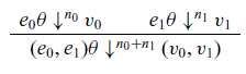
Cost  $n_i\leq {c_i}\{\Theta\}$ by the IH so $n_0+n_1\leq {c_0}\{\Theta\} + {c_1}\{\Theta\} = ({c_0+c_1})\{\Theta\}$. Value ${v_i}\preceq^{\mathrm{Val}}{{p_i}\{\Theta\}}$ by the IH so $({v_0},{v_1})\preceq^{\mathrm{Val}}(p_0\{\Theta\},p_1\{\Theta\})=(p_0,p_1)\{\Theta\}$ by the IH. $\underline{\mathrm{CASE:}\Gamma\vdash\pi_i e:\sigma_i}$ Fix $\theta\preceq^{\mathrm{Val}}_{\Gamma}\Theta$; we must show that $(\pi_i e)\theta \preceq(c,\pi_i p)\{\Theta\}=(c\{\Theta\},(\pi_i p)\{\Theta\})$, where ${\|e\|} = (c,p)$. The evaluation of ${\pi_i e}\theta$ has the form

Cost  $n\leq (c)\{\Theta\}$ by the IH.
Value  $(v_{0},v_{1})\preceq^{\mathrm{Val}}p\{\Theta\}$ by the IH, so $v_i \preceq^{\mathrm{Val}}\pi_i(p\{\Theta\})=(\pi_i, p)\{\Theta\}$ by the definition of $\preceq^{\mathrm{Val}}_{\sigma_{0}\times\sigma_{1}}$. $\underline{\mathrm{CASE:}\Gamma\vdash\iota_i e:\sigma_0+\sigma_1}$ Fix $\theta\preceq^{\mathrm{Val}}_{\Gamma}\Theta$; we must show that $(\iota_i e)\theta\preceq(c,\iota_i p)\{\Theta\}=(c\{\Theta\},(\iota_i p)\{\Theta\})$, where ${\|e\|} = (c, p)$. The evaluation of ${\iota_i e}\theta$ has the form

Cost  $n\leq c\{\Theta\}$ by the IH.
Value  $v\preceq^{\mathrm{Val}} {p\{\Theta\}}$ by the IH, and $\iota_i {(p\{\Theta\})}\leq \iota_i {(p\{\Theta\})}$, so ${\iota_i v}\preceq^{\mathrm{Val}} {\iota_i {(\{ \Theta\})}}= {\iota_i p}\{\Theta\}$ by the definition of $\preceq^{\mathrm{Val}}_{\sigma_0+\sigma_1}$. $\underline{\mathrm{CASE:}\Gamma\vdash\mathtt{case} e \mathtt{of}\{x.e\}_{i=0,1}:\sigma}$ Fix $\theta\preceq^{\mathrm{Val}}_{\Gamma}\Theta$; we must show that $(\mathtt{case} e \mathtt{of}\{x.e\}_{i=0,1})\theta\preceq(c+_c \mathtt{case} p \mathtt{of} \{(x:\langle\langle{\sigma_i}\rangle\rangle).(c_i,p_i)\}_{i=0,1})\{\Theta\}=c\{\Theta\}+_c \mathtt{case}p\{\Theta\}\mathtt{of}\{(x:\langle\langle{\sigma_i}\rangle\rangle).(c_i,p_i)\{\Theta-x\}\}_{i=0,1}$, where ${\|e\|} = (c,p)$ and $\|e_i\| = ({c_i,p_i})$. The evaluation of $(\mathtt{case} e \mathtt{of}\{x.e\}_{i=0,1})\theta$ has the form
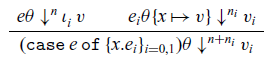
By the IH for e,  ${\iota_i v}\preceq^{\mathrm{Val}}{p \{\Theta\}}$, so there is some E’ such that $v\preceq^{\mathrm{Val}} E'$ and $\iota_i{E'}\leq p\{\Theta\}$. If we set $\theta' = {\theta}\{v\mapsto x\}$ and $\Theta' = {\Theta}\{E'/x\}$, then ${\theta'}\preceq^{\mathrm{Val}}{\Theta'}$, so by the IH for $e_i$, ${e_i}{\theta'}\preceq({c_i}\{\Theta'\},{p_i}\{\Theta'\})$. Since $\iota_i {E'} \leq p\{\Theta\}$, we have
 \begin{align*} ({{c_i}\{\Theta'\}},{p_i}\{\Theta'\}) &= {({c_i,p_i})}\{\Theta'\} \\ &\leq \mathtt{case} {\iota_i {E'}} \mathtt{of}\{(x:{\langle\langle{\sigma_i}\rangle\rangle}). {({c_i,p_i})\{\Theta-x\}}\}_{i=0,1} \\ &\leq \mathtt{case} {p\{\Theta\}} \mathtt{of} \{(x: {\langle\langle{\sigma_i}\rangle\rangle}). {({c_i,p_i})\{\Theta-x\}}\}_{i=0,1} \end{align*}
and so
 \begin{align*}(c\{\Theta\}+c_i\{\Theta'\},p_i\{\Theta'\})&=c\{\Theta\}+_c (c_i\{\Theta'\},p_i\{\Theta'\})&\leq c\{\Theta\}+_c\mathtt{case}p\{\Theta\} \mathtt{of} \{(x:\langle\langle{\sigma_i}\rangle\rangle).(c_i,p_i)\{\Theta-x\}\}_{i=0,1} \end{align*}
which we use to complete the next set of calculations.
Cost  $n\leq (c\{\Theta\})$ and $n_i\leq {c_i}\{\Theta'\}$, so
 \begin{align*} n+n_i &\leq c\{\Theta\} + {c_i}\{\Theta'\} \\ &\leq (c\{\Theta\}+{c_i}\{\Theta'\},p_i\{\Theta'\})_c \\ &\leq (c\{\Theta\}+_c\mathtt{case}p\{\Theta\} \mathtt{of} \{(x:\langle\langle{\sigma_i}\rangle\rangle).(c_i,p_i)\{\Theta-x\}\}_{i=0,1})_c. \end{align*}
Value
 \begin{align*} v_i &\preceq^{\mathrm{Val}} {p_i}\{\Theta'\} \\ &\leq (c\{\Theta\}+{c_i}\{\Theta'\},p_i\{\Theta'\})_p \\ &\leq (c\{\Theta\}+_c\mathtt{case}p\{\Theta\} \mathtt{of} \{(x:\langle\langle{\sigma_i}\rangle\rangle).(c_i,p_i)\{\Theta-x\}\}_{i=0,1})_p. \end{align*} $\underline{\mathrm{CASE:}\Gamma\vdash\lambda x.e:\sigma'\rightarrow\sigma}$ Fix $\theta\preceq^{\mathrm{Val}}_{\Gamma}\Theta$; we must show that ${(\lambda x.e)\theta}\preceq(0,\lambda(x:\langle\langle\sigma'\rangle\rangle).\|e\|)\{\Theta\}=(0,\lambda(x:\langle\langle\sigma'\rangle\rangle).\|e\|\{\Theta-x\})$. The evaluation of ${\lambda x.e}{\theta}$ has the form
so the cost claim is immediate.
Value Fix any  ${v'}\preceq^{\mathrm{Val}}{E'}$. We must show that $e\theta\{x\mapsto v'\}\preceq(\lambda(x:\langle\langle{\sigma'}\rangle\rangle).\|e\|\{\Theta-x\})E'$; by definition, $(\beta_\rightarrow)$, and Weakening, it suffices to show that $e\theta\{x\mapsto v'\}\preceq\|E\|\{\Theta\{x\mapsto E'\}\}$. Since $0\preceq^{\mathrm{Val}}\Theta$ and $v\preceq^{\mathrm{Val}}{E'}$, this follows from the induction hypothesis. $\underline{\mathrm{CASE:}\Gamma\vdash e_0 e_1:\sigma}$ Fix $\theta\preceq^{\mathrm{Val}}_{\Gamma}\Theta$. We must show that $(e_0 e_1)\theta \preceq((c_0+c_1)+_c p_0 p_1)\{\Theta\}$, where ${\|e_i\|} = ({c_i,p_i})$. The evaluation of $({e_0,e_1})\theta$ has the form

By the IH,  $n_0\leq {c_0}\{\Theta\}$, ${\lambda x.{e_0'}}{\theta'}\preceq^{\mathrm{Val}}{{p_0}\{\Theta\}}$, $n_1\leq {c_1}\{\Theta\}$, and ${v_1}\preceq^{\mathrm{Val}}{{p_1}\{\Theta\}}$. By definition of $\preceq^{\mathrm{Val}}$, $e'_{0}\Theta'\{x\mapsto v_1\}\preceq(p_0\{\Theta\})(p_1\{\Theta\})=(p_0 p_1)\{\Theta\}$, so $n\leq ((p_0 p_1)\{\Theta\})$ and $v\preceq^{\mathrm{Val}}((p_0 p_1)\{\Theta\})_p$.
Cost  $n_0 + n_1 + n \leq c_0\{\Theta\}+c_1\{\Theta\}+((p_0 p_1)\{\Theta\})_c \leq(((c_0+c_1)+_c p_0 p_1)\{\Theta\})_c$.
Value  $v\preceq^{\mathrm{Val}}((p_0 p_1)\{\Theta\})_p \leq(((c_0+c_1)+_c p_0 p_1)\{\Theta\})_p$. $\underline{\mathrm{Case:}\Gamma\vdash\mathtt{delay}e:\sigma\mathtt{susp}}$ Fix $\theta\preceq^{\mathrm{Val}}_{\Gamma}\Theta$. We must show that $(\mathtt{delay} e)\theta \preceq(0,\|e\|)\{\Theta\}=(0,\|e\|\{\Theta\})$. The evaluation of $(\mathtt{delay} e)\theta$ has the form
so (cost)  $0\leq 0$ and (value) since ${e\theta}\preceq{{\|e\|}\{\Theta\}}$ by the IH, $(\mathtt{delay}e)\theta \preceq^{\mathrm{Val}}\|e\|\{\Theta\}$ by the definition of $\preceq^{\mathrm{Val}}_{\sigma\mathtt{susp}}$. $\underline{\mathrm{Case:}\Gamma\vdash\mathtt{force}e:\sigma}$ Fix $\theta\preceq^{\mathrm{Val}}_{\Gamma}\Theta$. We must show that $(\mathtt{force}e)\theta\preceq(c+_c p)\{\Theta\}$, where ${\|e\|} = (c,p)$. The evaluation of $(\mathtt{force}e)\theta$ has the form

By the IH,  $n\leq c\{\Theta\}$ and $(\mathtt{delay}e')\theta' \preceq^{\mathrm{Val}} p\{\Theta\}$, so by definition of $\preceq^{\mathrm{Val}}$, $e'\theta'\preceq p\{\Theta\}$ and hence $n' \leq (p\{\Theta\})_c$ and $v\preceq^{\mathrm{Val}}(p\{\Theta\})_p$. So (cost) $n+n' \leq c\{\Theta\} + p\{\Theta\} \leq((c+_c p)\{\Theta\})_c$ and (value) $v\preceq^{\mathrm{Val}}p\{\Theta\}_p\leq((c+_c p)\{\Theta\})_p$. $\underline{\mathrm{Case:}\Gamma\vdash\mathtt{c}_{\delta}e:\sigma}$ Fix $\theta\preceq^{\mathrm{Val}}_{\Gamma}\Theta$. We must show that $(\mathtt{c}_\delta e)\theta\preceq(c,\mathtt{c}_{\langle\langle{\delta}\rangle\rangle}p)\{\Theta\}$, where ${\|e\|} = (c,p)$. The evaluation of $(\mathtt{c}_\delta e)\theta$ has the form

Cost  $n\leq c\{\Theta\}$ by the IH.
Value By the IH we have that  $v\preceq^{\mathrm{Val}}_{\langle\langle{F}[\delta]\rangle\rangle} p\{\Theta\}$, and so by Lemma 2, $v\preceq^{\mathrm{Val}}_{F,\delta}p\{\Theta\}$. Since $\mathtt{c}_{\langle\langle{\delta}\rangle\rangle}p\leq\mathtt{c}_{\langle\langle\delta\rangle\rangle}p$, the value bound follows by definition of $\preceq^{\mathrm{Val}}_{\delta}$. $\underline{\mathrm{Case:}\Gamma\vdash\mathtt{d}_{\delta}e:F[\delta]}$ Fix $\theta\preceq^{\mathrm{Val}}\Theta$. We must show that $(\mathtt{d}_{\delta}e)\theta\preceq(c,\mathtt{d}_{\langle\langle\delta\rangle\rangle}p)\{\Theta\}=(c\{\Theta\},\mathtt{d}_{\langle\langle\delta\rangle\rangle}(p\{\Theta\}))$, where ${\|e\|} = (c,p)$. The evaluation of $(\mathtt{d}_{\delta} e)\theta$ has the form
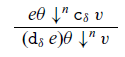
Cost  $n\leq c\{\Theta\}$ by the IH.
Value By the IH,  $\mathtt{c}_{\delta}v\preceq^{\mathrm{Val}} p\{\Theta\}$, and so by definition of $\preceq^{\mathrm{Val}}_{\delta}$, there is E such that $v\preceq^{\mathrm{Val}}_{F,\delta}E$ and $\mathtt{c}_{\langle\langle{\delta}\rangle\rangle}E\leq p\{\Theta\}$. This latter fact along with the axioms for $\leq$ tell us that $E \leq\mathtt{d}_{\langle\langle{\delta}\rangle\rangle}(\mathtt{c}_{\langle\langle{\delta}\rangle\rangle} E) \leq \mathtt{d}_{\langle\langle{\delta}\rangle\rangle} (p\{\Theta\})$. $\underline{\mathrm{CASE:}\Gamma\vdash\mathrm{fold}_{\delta}e' \mathtt{of} x.e:\sigma}$ The type derivation has the form

Fix  $\theta\preceq^{\mathrm{Val}}_{\Gamma}\Theta$ and without loss of generality assume that $x\notin\mathrm{Dom}\;\Gamma\cup\mathrm{Dom}\;\theta\cup\mathrm{Dom}\;\Theta$; we must show that $(\mathtt{fold}_\delta e' \mathtt{of} x.e)\theta\preceq c' +_c \textsf{fold}_{\langle\langle{\delta}\rangle\rangle}p' \mathtt{of}(x:\langle\langle F\rangle\rangle[\|\sigma\|]).1+_c \|e\|$ where $\|e'\| = (c', p')$. The evaluation of $(\mathtt{fold}_{\delta}e' \mathtt{of}x.e)\theta$ has the form

and so the following is also an evaluation, where we write  $\theta'$ for $\theta\{z\mapsto \mathtt{c}_{\delta}v'\}$:
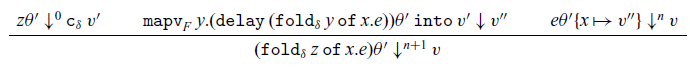
The IH for e’ tells us that  $n'\leq {c'}\{\Theta\}$ and $\mathtt{c}_{\delta}v' \preceq^{\mathrm{Val}}p'\{\Theta\}$; combined with the IH for e, Lemma 16 tells us that $(\mathtt{fold}_{\delta} z \mathtt{of} x.e)\theta' \preceq\textsf{fold}_{\langle\langle{\delta}\rangle\rangle}p'\{\Theta\}\mathtt{of}(x:\langle\langle{F}\rangle\rangle[\|\sigma\|]).1+_c \|e\|\{\Theta\}$ as required. $\underline{\mathrm{CASE:}\Gamma\vdash\mathtt{let}x=e' \mathtt{in} e: \sigma}$ The type derivation has the form
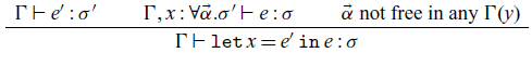
Fix  $\theta\preceq^{\mathrm{Val}}_{\Gamma}\Theta$ and without loss of generality assume x is fresh for $\Gamma$, $\theta$, and $\Theta$ and that no $\alpha_i$ is free in any $\Theta(y)$. We must show that $(\mathtt{let}x=e' \mathtt{in} e)\theta\preceq(c'+_c \|e\|\{\Lambda\vec{\alpha}.p'/x\})\{\Theta\}=c'\{\Theta\}+_c \|e\|\{\Theta\}\{\Lambda\vec{\alpha}.p'\{\Theta\}/x\}$ where $\|e'\| = (c', p')$. The evaluation has the form
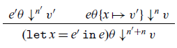
The IH for e’ tells us that  $n'\leq {c'}\{\Theta\}$ and ${v'}\preceq^{\mathrm{Val}}_{\sigma'}{{p'}\{\Theta\}}$. If we can show that $v'\preceq^{\mathrm{Val}}_{\forall\vec{\alpha}.\sigma'}\Lambda\vec{\alpha}.p'\{\Theta\}$, then the induction hypothesis applied to e provides the remaining pieces of the argument. For this we need to show that for any closed $\vec\rho$, $v'\preceq^{\mathrm{Val}}_{\sigma'\{\vec{\rho}/\vec{\alpha}\}}(\Lambda\vec{\alpha}.p'\{\Theta\})\langle\langle{\vec{\rho}}\rangle\rangle$, and by $(\beta_\forall)$ and weakening, it suffices to show $v'\preceq^{\mathrm{Val}}_{\sigma'\{\vec{\rho}/\vec{\alpha}\}}p'\{\Theta\}\{\langle\langle\vec{\rho}\rangle\rangle/\vec{\alpha}\}$. This in turn requires us to show that if $\mathrm{ftv}(\sigma) = \{\vec{\alpha},\vec{\beta}\}$, then for any closed $\vec{\rho'}$, $v'\preceq^{\mathrm{Val}}_{\sigma'\{\vec{\rho},\vec{\rho'}/\vec{\alpha},\vec{\beta}\}}p'\{\Theta\}\{\langle\langle\vec{\rho},\vec{\rho'}\rangle\rangle/\vec{\alpha},\vec{\beta}\}$, which follows from the fact that $v'\preceq^{\mathrm{Val}}_{\sigma'}p'\{\Theta\}$.


 Open access
Discussions
No Discussions have been published for this article.