


1. Introduction
The sound of flutes is produced through aeroacoustic instabilities that result from the constructive feedback between the acoustic modes of the instruments and the dynamics of a shear layer (Fabre et al. Reference Fabre, Gilbert, Hirschberg and Pelorson2011). These instabilities also cause numerous issues in industry because they can induce significant noise pollution and unwanted vibrations leading to fatigue failures (Ziada & Lafon Reference Ziada and Lafon2014). They have been investigated over several decades and they fall into the category of fluid-resonant cavity flows in the classification established by Rockwell & Naudascher (Reference Rockwell and Naudascher1978). This type of instability can be further divided into two groups: the self-sustained flow oscillations in shallow cavities (Rowley & Williams Reference Rowley and Williams2006), and the ones of deep cavities (Tonon et al. Reference Tonon, Hirschberg, Golliard and Ziada2011a).
In the former group, the unsteady cavity flows are governed by the mechanism of Rossiter (Reference Rossiter1964) and they are particularly relevant for aeronautic applications of high subsonic and low supersonic grazing flows. Canonical configurations have been investigated numerically with dynamic systems and control theory (e.g. Illingworth, Morgans & Rowley Reference Illingworth, Morgans and Rowley2012), and with computational aeroacoustics methods, which are based on direct numerical simulations and large eddy simulations (LES) of the compressible Navier–Stokes equations (e.g. Rowley, Colonius & Basu Reference Rowley, Colonius and Basu2002; Gloerfelt, Bailly & Juvé Reference Gloerfelt, Bailly and Juvé2003; Yokoyama & Kato Reference Yokoyama and Kato2009) or on the linearization of these equations around a given base flow (e.g. Yamouni, Sipp & Jacquin Reference Yamouni, Sipp and Jacquin2013; Sun et al. Reference Sun, Taira, Cattafesta and Ukeiley2017).
In the latter group, to which belongs the aeroacoustic instability investigated in this work, the self-sustained flow oscillations involve the longitudinal acoustic eigenmodes of the deep cavity. These instabilities are usually relevant for low-Mach grazing flows and their modelling has been the topic of intense research over several decades. Most of the investigations considered the canonical problem of a single deep cavity, while some works deal with multiple deep cavities (e.g. Tonon, Willems & Hirschberg Reference Tonon, Willems and Hirschberg2011b; Dai & Aurégan Reference Dai and Aurégan2018) and liners made of deep cavities equipped with perforated plates (Dai Reference Dai2020). There are also several studies dealing with various passive control methods to prevent whistling of a deep cavity, such as flow obstacles inside the cavity (Matsuura & Nakano Reference Matsuura and Nakano2014), an internal cavity liner (Hong et al. Reference Hong, Dai, Zhou, Sun and Jing2014) or changes of the curvature of the cavity opening corners (Wang, He & Liu Reference Wang, He and Liu2020).
Many of the studies focusing on single deep cavities, including the present investigation, follow the work of Elder (Reference Elder1978), who proposed a feedback loop analysis with the cavity opening and its aerodynamic forcing as a forward transfer function and the acoustic resonance of the deep cavity as a backward transfer function. For example, Mast & Pierce (Reference Mast and Pierce1995) and Kook & Mongeau (Reference Kook and Mongeau2002), who used a frequency-domain describing function analysis to predict the occurrence and the amplitude of deep cavity whistling. Another example is Marsden et al. (Reference Marsden, Bailly, Bogey and Jondeau2012), who used the same approach in combination with particle image velocimetry (PIV) in the central plane of their cylindrical cavity.
A key element of this type of analysis is the forward transfer function, which is governed by the unsteady vorticity–velocity cross-product, as pointed out by Howe (Reference Howe1980) and Nelson, Halliwell & Doak (Reference Nelson, Halliwell and Doak1983) about 40 years ago. The analytical models of this transfer function can be grouped into two categories: the ones based on the work of Howe (Reference Howe1997), which considers the shear layer as a thin vortex sheet, and the ones that are based on discrete vortices that are periodically shed from the upstream corner of the cavity (Nelson et al. Reference Nelson, Halliwell and Doak1983). One can for instance refer to the papers of Bruggeman et al. (Reference Bruggeman, Hirschberg, Van Dongen, Wijnands and Gorter1991) or Dequand, Hulshoff & Hirschberg (Reference Dequand, Hulshoff and Hirschberg2003) in which the latter formulation is adopted. Dequand et al. (Reference Dequand, Hulshoff and Hirschberg2003) also compared against simulations of the compressible Euler equations and results from the vortex blob method of Peters & Hoeijemakers (Reference Peters and Hoeijemakers1995). More recently, Ma, Slaboch & Morris (Reference Ma, Slaboch and Morris2009) used particle image velocimetry to show that shear layers do not appear as either a flapping vortex sheet or discrete vortices, but rather as a combination of these two ideals, which depends on the grazing flow velocity and on the self-sustained oscillation amplitude. While several studies concentrate on a frequency-domain oriented analysis, there are also some investigations focusing on time-domain simulations and transients, which are particularly relevant for music instruments (e.g. Verge, Hirschberg & Caussé Reference Verge, Hirschberg and Caussé1997; Terrien, Vergez & Fabre Reference Terrien, Vergez and Fabre2013). Semi-empirical models of the forward transfer function can also be directly derived from measurements of the impedance of the cavity opening and its shear layer (e.g. Graf & Ziada Reference Graf and Ziada2010; Karlsson & Åbom Reference Karlsson and Åbom2010). Finally, it is important to mention that one can use various computational methods to identify the aeroacoustic response of the cavity opening. A first example is the paper of Martínez-Lera et al. (Reference Martínez-Lera, Schram, Föller, Kaess and Polifke2009), in which the forward transfer function is obtained from incompressible flow simulations, vortex sound theory and system identification techniques. In fact, for sufficiently low frequencies, the cavity opening is acoustically compact and the unsteady flow can be locally considered and simulated as incompressible. Another example is the work of Gikadi, Föller & Sattelmayer (Reference Gikadi, Föller and Sattelmayer2014), where the compressible Navier–Stokes equations are linearized around a mean grazing flow obtained from LES and where the forward transfer function and transfer matrices are successfully compared with the experiments from Karlsson & Åbom (Reference Karlsson and Åbom2010). One can also refer to the paper of Boujo, Bauerheim & Noiray (Reference Boujo, Bauerheim and Noiray2018), who considered the incompressible Navier–Stokes equations linearized around mean flows of the acoustically forced cavity opening. The latter mean flows were obtained from LES for a range of acoustic forcing amplitudes, in order to demonstrate that the forward transfer functions can be extracted with this method in the linear regime, but also in the saturated nonlinear regime.
In the present work the forward and backward transfer functions are measured for ranges of grazing flow velocities, cavity depths and acoustic amplitudes, and used for deriving a new low-order model of the aeroacoustic system in the form of two coupled oscillators. This formulation allows us to revisit this classic problem and to provide novel insights into the underlying deterministic and stochastic dynamics. This nonlinear model is used for frequency-domain describing function analysis as well as for performing time-domain simulations and for deriving amplitude and phase equations. We also add stochastic forcing terms to this low-order predictive model to represent the effect of turbulence on the aeroacoustic instability. In fact, the unsteady component of the flow in deep cavities subject to turbulent grazing flows can be decomposed as turbulent fluctuations and coherent fluctuations. The recent experimental works of Ishikawa et al. (Reference Ishikawa, Tanigawa, Yatabe, Oikawa, Onuma and Niwa2018) and of Boujo et al. (Reference Boujo, Bourquard, Xiong and Noiray2020) show the coexistence of these two types of fluctuations in the case of a whistle and of a bottle. We will focus on the fact that our aeroacoustic oscillations are intermittent for some combinations of turbulent grazing flow velocity and cavity depth. Intermittency in dynamical systems has received considerable attention. In the case of thermoacoustic instabilities, one can for instance refer to the early work of Clavin, Kim & Williams (Reference Clavin, Kim and Williams1994) or to the more recent studies from Nair, Thampi & Sujith (Reference Nair, Thampi and Sujith2014) or from Bonciolini et al. (Reference Bonciolini, Ebi, Boujo and Noiray2018). Many of the investigations dealing with intermittency of thermoacoustic systems concentrate on noise-driven subcritical Hopf bifurcations. We will show in the present paper that thermoacoustic and aeroacoustic configurations exhibiting supercritical Hopf bifurcations can also exhibit intermittency, with similar acoustic pressure statistics that correspond to sporadic bursts of high-amplitude oscillations, but with a very different dynamical signature. Indeed, we will show that the present aeroacoustic system can be intermittently unstable, as in the systems investigated by Mohamad & Sapsis (Reference Mohamad and Sapsis2015), and we will identify the necessary conditions for observing this intermittency.
The experimental set-up and the aeroacoustic instability are introduced in § 2. The specific acoustic admittance of the deep cavity and the specific acoustic impedance of its opening with and without grazing flow are presented in §,3, together with the linear model of coupled oscillators and the analysis of its eigenvalues. In § 4, the nonlinear problem is treated with a describing function analysis as well as with amplitude equations. Finally, the experimental and theoretical analysis of the intermittency at play in the present aeroacoustic system is investigated in § 5.
2. Experimental set-up and aeroacoustic instability
The system considered in the present work consists of a two metre long wind channel with a square cross-section of side  $H=62$ mm, which is supplied by a blower and is operated at atmospheric pressure. The temperature in the channel is maintained constant at $23\,^{\circ }\textrm {C}$ with a heat exchanger located immediately downstream of the blower, which corresponds to a speed of sound in the channel $c$ of $345\ \textrm {m}\ \textrm {s}^{-1}$. The bulk flow velocity $U$ in the channel is varied between 35 and $75\ \textrm {m}\ \textrm {s}^{-1}$, respectively corresponding to Reynolds numbers $Re=UH/\nu =145\,000$ and $310\,000$, where $\nu =1.5\times 10^{-5}\ \textrm {m}^{2}\ \textrm {s}^{-1}$ is the kinematic viscosity of the air. The bulk velocity is deduced from the mass flow and the temperature in the channel, which are respectively measured with a Bronkhorst IN-FLOW F-106CI and a thermocouple. A side-branch cavity is located in the middle of the channel, as shown in figure 1. This rectangular cuboid spans across one of the channel sides, exhibits a cross-section $W\times H$ with $W=30$ mm and its length $L$ can be varied using a tight piston. Large plenums ( $0.5\ \textrm {m}\times 0.7\ \textrm {m}\times 0.7\ \textrm {m}$) equipped with sound absorbing foam and catenoid horns are mounted at both ends of the channel in order to create anechoic conditions upstream and downstream of the side-branch cavity. The corresponding cutoff frequency is approximately 300 Hz, and the upstream and downstream reflection coefficients drop below 0.1 beyond that frequency. The coordinate system is defined as follows: the $x$ axis points in the direction of the flow, and the $y$ axis inside the deep cavity, with the origin set in the middle of the junction. A turbulent shear layer develops between the main channel and the side-branch cavity. Depending on the mean flow velocity $U$ and the cavity length $L$, an aeroacoustic instability can occur due to a constructive feedback between the acoustic modes of the cavity and the aerodynamic modes of the shear layer.

Figure 1. Sketch of the experimental set-up used to investigate the side-branch cavity whistling. The system is broken down into two subsystems: the deep cavity and the interface between the cavity and the channel along which the shear layer develops.
In the present study, the cavity length  $L$ is varied between 200 and 270 mm, and the acoustic mode of the cavity, which is involved in the aeroacoustic instability, is the three-quarter wave eigenmode, with its eigenfrequency being close to $f_a=3c/4L$. For this range of length, the cavity length-to-width ratio $L/W$ is approximately 8 and therefore the configuration falls into the category of deep cavity whistling. Four G.R.A.S. 46BD $1/4''$ CCP microphones are flush mounted on the internal wall of the cavity, at $y=0$, 45, 90 and 190 mm. The full set of microphones is used for the measurements of the reflection coefficient presented in the next section. The acoustic pressure time traces used to characterize the aeroacoustic instability were recorded with the third microphone, which is located in the vicinity of a pressure antinode of the three-quarter wave mode for the considered range of length $L$.
$L$.
The length of the deep cavity is first fixed to  $L=250$ mm and the power spectral density $S_{pp}$ of the acoustic pressure $p$ at $y=90$ mm is measured for a range of mean flow velocity, $U$, between 35 and $75\ \textrm {m}\ \textrm {s}^{-1}$. This mapping is presented in figure 2(a). One can see in figure 2(b) that for $U=74\ \textrm {m}\ \textrm {s}^{-1}$, the power spectral density of the acoustic pressure exhibits a sharp high-amplitude peak at approximately 980 Hz, which is the signature of a strong aeroacoustic limit cycle. Its harmonic at 1960 Hz is also visible in the power spectral density. This limit cycle involves the three-quarter wave acoustic eigenmode of the deep cavity, whose natural eigenfrequency can be approximated by $3c/4L_e=987$ Hz, where $L_e$ is the sum of the physical length $L=250$ mm, and an end correction of 12 mm (see § 3.1 for a short discussion about this correction). From figure 2(a), one can clearly see the signature of the three-quarter, five-quarter and seven-quarter wave pure acoustic modes (estimated at 987 Hz, 1645 Hz and 2303 Hz respectively) on the left side of the map, i.e. for low velocity for which the shear layer does not significantly interact with these acoustic modes. The raw acoustic pressure time trace for $U=74\ \textrm {m}\ \textrm {s}^{-1}$ is shown in figure 2(c). It can be decomposed into two main components: slow fluctuations, which correspond to the high-amplitude low-frequency content of the power spectral density (below 200 Hz), and fast fluctuations originating from the aeroacoustic instability of the deep cavity. The low-frequency content originates from the blower and the natural aeroacoustic sources of the air supply line, as indicated in the acoustic power spectral density in the channel and in the absence of a cavity, which is shown in figure 2(b). In order to isolate the dynamics of the aeroacoustic limit cycle, the acoustic pressure signal is band-pass filtered with a 200 Hz bandwidth centred on the main peak (see shaded region in figure 2b). In the next figures showing time traces and probability density functions of the acoustic pressure from experiments, the signals are filtered in this way. The filtered time trace for $U=74\ \textrm {m}\ \textrm {s}^{-1}$ is shown in figure 2(d) and it features a slowly varying amplitude modulation that is typical of a self-sustained weakly nonlinear oscillator subject to random forcing.

Figure 2. (a) Mapping of the power spectral density of the acoustic pressure  $S_{pp}$ recorded in the cavity at $y=90$ mm for mean bulk flow velocities in the wind channel ranging from 35 to $75\ \textrm {m}\ \textrm {s}^{-1}$, and for a fixed cavity length $L=250$ mm. (b) Blue line: $S_{pp}$ in the cavity at $y=90$ mm for $U=74\ \textrm {m}\ \textrm {s}^{-1}$. Grey line: $S_{pp}$ in the wind channel at $y=-31$ mm for the same velocity, but without cavity, i.e. $L=0$ (the piston is flush to the wind channel wall). (c) Raw acoustic pressure time trace at $y=90$ mm, for $L=250$ mm and $U=74\ \textrm {m}\ \textrm {s}^{-1}$. (d) Band-pass filtered acoustic pressure (inverse Fourier transform of the shaded area in panel b).
In order to get insights into the aeroacoustic feedback at play in these self-sustained oscillations, PIV is used to characterize the dynamics of the shear layer. The use of PIV for characterizing the shear layer dynamics of unsteady cavity flows has been reviewed by Morris (Reference Morris2011). It is here combined with acoustic records to perform phase averaging of the velocity field in the shear layer region, which is optically accessible through two quartz windows, as shown in figure 3. These PIV measurements are made using a double cavity laser (Photonics DM60Nd:YAG, 532 nm), a laser guiding arm, sheet optics and a HighSpeedStar X camera from Lavision. The camera is equipped with a Nikon 100F/2.8D lens and a 36 mm extension ring, and it is placed perpendicularly to the laser sheet formed in the central plane of the channel. The seeding of the flow is achieved with a spray of di-ethyl-hexyl-sebacat in the inlet plenum. A measurement of 2500 double-frame images at a rate of 5 kHz with time interval of  $10\ \mathrm {\mu }\textrm {s}$ between pairs of consecutive laser pulses is performed in combination with the recording of acoustic signal at 50 kHz sampling rate.
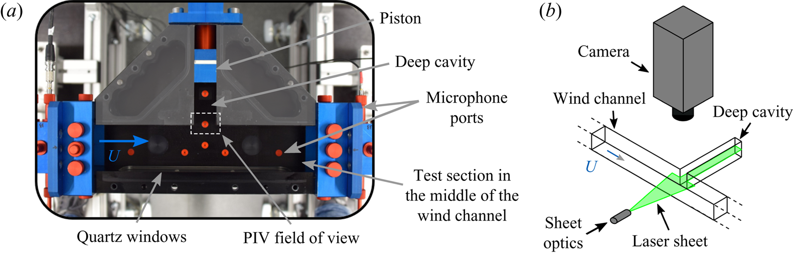
Figure 3. (a) Picture of the test section placed in the middle of the wind channel. The length  $L$ of the side-branch cavity is adjusted with the piston. The PIV field of view, which encompasses the turbulent shear layer, is indicated with the dotted line rectangle. (b) Sketch of the experimental set-up used for PIV measurements.
The trigger of the camera and the acoustic pressure signal are used to assign to each Mie-scattering image its corresponding phase angle with respect to the self-sustained aeroacoustic oscillations. Instantaneous snapshots of the velocity magnitude  $|\boldsymbol {v}|$ are presented in the top row of figure 4 and show the presence of small scale turbulent structure along the shear layer. Phase averaging was performed by considering instantaneous velocity fields falling in the same phase bin in order to remove the zero-mean turbulent component of the velocity $\check {\boldsymbol {v}}$. The magnitude of the resulting phase-averaged component of the velocity $|\langle \boldsymbol {v}\rangle |$ is shown in the middle row of figure 4. One can observe that there is no coherent vortex shedding from the upstream corner. In fact, the shear layer exhibits a hardly discernible low-amplitude coherent flapping motion, despite the intense sound level ( ${\approx }130$ dB) in the cavity that results from this aeroacoustic limit cycle. These results indicate that the assumption of a thin vortex sheet (Howe Reference Howe1997) should be adequate to describe the present aeroacoustic limit cycle. The mean component of the velocity field $\bar {\boldsymbol {v}}$, which is obtained by averaging the 2500 instantaneous fields, is then subtracted from the phase-averaged velocity fields $\left \langle \boldsymbol {v}\right \rangle$ in order to extract the zero-mean coherent component of the velocity fluctuations $\tilde {\boldsymbol {v}}$. Note that these notations correspond to the following decompositions of the total velocity field: $\boldsymbol {v} = \bar {\boldsymbol {v}} + \tilde {\boldsymbol {v}} + \check {\boldsymbol {v}} = \left \langle \boldsymbol {v}\right \rangle +\check {\boldsymbol {v}}= \bar {\boldsymbol {v}} + \boldsymbol {v}'$, where $\boldsymbol {v}'$ are the zero-mean fluctuations. The vector field $\tilde {\boldsymbol {v}}$ is presented in the bottom row of figure 4 together with the magnitude of the vertical coherent velocity fluctuations. It shows that the constructive aeroacoustic feedback involves the first longitudinal hydrodynamic mode whose wavelength is close to the cavity width $W$. The nonlinear response of this aerodynamic eigenmode to transverse acoustic forcing has been investigated numerically by Boujo et al. (Reference Boujo, Bauerheim and Noiray2018) with the same geometry but at a lower bulk flow velocity ( $U=56\ \textrm {m}\ \textrm {s}^{-1}$). It is worth mentioning that in the present configuration, knowledge of the full time-dependent flow by PIV is not sufficient to quantitatively predict the forward transfer function of the aeroacoustic problem. This is because the PIV only offers partial information about the cavity flow: the sidewalls induce three-dimensional (3-D) dynamics in the shear layer oscillation, which cannot be deduced from the PIV data that are only available in the central plane.

Figure 4. Combined PIV and acoustic data processing for characterizing the shear layer dynamics of the aeroacoustic limit cycle occurring when  $L=250$ mm and $U=74\ \textrm {m}\ \textrm {s}^{-1}$. (a) Instantaneous velocity magnitude $|\boldsymbol {v}|$ at 5 regularly spaced instants of an acoustic period. (b) Phase-averaged velocity magnitude $|\langle \boldsymbol {v}\rangle |$. (c) Vector field of the zero-mean coherent component of the velocity fluctuations $\tilde {\boldsymbol {v}}$ coloured by its vertical amplitude $\tilde {v}_y$. Movies can be seen in the supplementary material available at https://doi.org/10.1017/jfm.2020.984.
3. Linear model of coupled oscillators
In this section, a linear model is derived to describe the aeroacoustic instability. As shown in the sketch on the right of figure 1, the aeroacoustic system is broken into two coupled subsystems: the deep cavity and the cavity opening subject to the turbulent grazing flow. The acoustic velocity  $\tilde {\boldsymbol{u} }$ is the irrotational part of the zero-mean coherent component of the velocity, and in the remainder of the paper, we focus on its vertical component at the opening $\tilde {u}_y$, which we will just denote $u$. In § 3.1, measurements of the specific acoustic admittance of the deep cavity $\mathcal {A}=\rho c \hat {u}/\hat {p}$ and of the specific acoustic impedance of the cavity opening $\mathcal {Z}=\hat {p}/\rho c \hat {u}$, are conducted and serve as a basis for the model derivation. In these expressions, $\rho$ denotes the air density and $\hat {\cdot }$ stands for the frequency-domain formulation for the acoustic velocity $\hat {u}$ and pressure $\hat {p}$ at the cavity opening.
3.1. Impedance measurements and model derivation
Measurements of  $\mathcal {Z}$ and $\mathcal {A}$ are made using the experimental set-ups respectively shown in figures 5(a) and 5(b). Acoustic forcing is applied with loudspeakers and the multi-microphone method (Schuermans et al. Reference Schuermans, Bellucci, Guethe, Meili, Flohr and Paschereit2004) is used to reconstruct the amplitude and phase of the forward and backward acoustic Riemann invariants $f$ and $g$, with which the reflection coefficient $\mathcal {R}$ and the specific impedance or admittance at a reference plane are deduced. The specific impedance of the cavity opening $\mathcal {Z}$ and the specific admittance of the deep cavity $\mathcal {A}$, which are measured with this method, are respectively presented in figures 6(a) and 6(b) for several bulk flow velocities $U$, and in figures 6(c) and 6(d) for several cavity lengths $L$. The white circles correspond to the specific impedance $\mathcal {Z}$ without flow. In that case, the specific resistance $\textrm {Re}(\mathcal {Z})$ is rather constant and it is equal to approximately 0.25 for the considered frequency range. This can be explained by considering the analogy between the travelling acoustic waves $f$ and $g$ in the side-branch cavity (see figure 5a) and the ones travelling toward and from an idealized compact area expansion in a duct. In the latter configuration, the amplitude reflection and transmission coefficients are respectively given by $\mathcal {R}=(\varepsilon -1)/(\varepsilon +1)$ and $\mathcal {T}=2\varepsilon /(\varepsilon +1)$, and the specific impedance is $\mathcal {Z}=\varepsilon$, where $\varepsilon$ is the area ratio at the sudden area expansion. In the present configuration, one can approximate the effective area expansion as the ratio between the cavity cross-section $WH$ and twice the wind channel cross-section $2H^{2}$, because acoustic energy originating from the cavity is transmitted in both the upstream and downstream directions of the channel. This leads to $\varepsilon \approx W/2H = 0.24$, which is very close to the measured specific acoustic resistance. In contrast with the real valued $\mathcal {Z}=\varepsilon$, the measured specific reactance is not zero. This is due to the fact that the inertia of the air at the cavity opening is not accounted for. The inertia of this attached air mass can be modelled as a fictive length of the cavity opening, based on the momentum balance $\rho \delta HW s \hat {u} = HW \hat {p}$, where $s=\textrm {i}\omega$ is the Laplace variable ( $\omega =2{\rm \pi} f$ is the angular frequency), and the so-called end correction $\delta$ represents the fictive length of the cavity opening. From this balance, one has $\textrm {Im}(\mathcal {Z})=\omega \delta /c$, and, as explained in § 6.7 of Rienstra & Hirschberg (Reference Rienstra and Hirschberg2012), this end correction is of the order of the hydraulic radius of the cavity opening, which is approximately 25 mm in the present geometry. Based on the linear trend of the measured specific reactance of the opening without flow (white circles in figure 6b), one can deduce that $\delta \simeq 12$ mm.

Figure 5. (a) Experimental set-up for measuring the reflection coefficient  $\mathcal {R}$, which is the ratio of the forward and backward acoustic Riemann invariants $f$ and $g$, and the specific impedance $\mathcal {Z}$ of the interface between the cavity and the channel along which the shear layer develops. (b) Experimental set-up for measuring the specific admittance of the deep cavity $\mathcal {A}$.

Figure 6. (a,b) Specific resistance  $\textrm {Re}(\mathcal {Z})$ and reactance $\textrm {Im}(\mathcal {Z})$ of the cavity opening along which the shear layer develops for several bulk flow velocities $U$. The black lines correspond to the fits based on (3.1). The red dotted line in (a) highlights the presence of frequency ranges for which the resistance is negative, which means that reflected waves $g$ exhibit higher amplitude than incident waves $f$ (necessary condition for an aeroacoustic instability in the configuration of figure 1). (c,d) Modulus and phase of the specific admittance of the deep cavity for different lengths $L$. The black lines correspond to the fits based on (3.2).
In presence of the shear layer, the specific impedance of the cavity opening is significantly affected. One can see in figures 6(a) and 6(b) that the specific resistance and reactance both exhibit a frequency dependence oscillating around the values obtained without channel flow, which is typical of the impedance of side branches subject to grazing flow, e.g. Karlsson & Åbom (Reference Karlsson and Åbom2010). This is due to the response of the first longitudinal aerodynamic mode to the incident acoustic wave of complex amplitude  $f$. Further insights into the nonlinear aerodynamic response of this shear layer when it is subject to incident acoustic waves are provided in the study of Boujo et al. (Reference Boujo, Bauerheim and Noiray2018). One can see in figure 6(a) that, for each velocity $U$, there exists a resistance minimum, which corresponds to the eigenfrequency $f_1$ of this aerodynamic eigenmode. The frequency of the minimum of $\textrm {Re}(\mathcal {Z})$ increases linearly with the flow velocity, scaling with the Strouhal number $St_1= f_1W/U\approx 0.4$, which has been already observed in several works on the topic, e.g. Dequand et al. (Reference Dequand, Hulshoff and Hirschberg2003). This corresponds to flow perturbations originating from the upstream corner that travel at approximately $0.4U$ across the opening during one acoustic oscillation cycle. The advection speed of the perturbations is roughly equal to the mean value of the velocity across the shear layer, which ranges from very low velocities in the cavity to the bulk velocity $U$ in the mean channel (see figure 4). It is important to note that the specific resistance minimum becomes negative for velocities exceeding $65\ \textrm {m}\ \textrm {s}^{-1}$. In fact, when the reflection coefficient satisfies $|\mathcal {R}|=|g/f|>1$, then $\textrm {Re}(\mathcal {Z})<0$, which is a necessary condition for self-sustained aeroacoustic oscillations in the configuration presented in figure 1. This occurs (i) if the time and spatially averaged projection of the unsteady component of the Lamb vector $(\boldsymbol {\omega }\times \boldsymbol {v})'$ onto the acoustic field is positive ( $\boldsymbol {\omega }=\boldsymbol {\nabla }\times \boldsymbol {v}$ is the vorticity), which corresponds to acoustic energy production according to Howe's energy corollary (Howe Reference Howe1980), and (ii) if this acoustic energy production exceeds the radiation losses in the wind channel. Readers interested by the space–time evolution of the unsteady component of the Lamb vector in a similar configuration (self-sustained aeroacoustic oscillations of a bottle whose neck is subject to a grazing flow) can refer to the recent work of Boujo et al. (Reference Boujo, Bourquard, Xiong and Noiray2020). In the present study, the measured specific impedance is fitted using the following second-order transfer function
 \begin{equation} \mathcal{Z}(s) = \frac{\hat{p}}{\rho c \hat{u}} = n\frac{s^{2} + 2m s + \omega_l^{2}}{s^{2} +2 d s + \omega_r^{2}}, \end{equation}
with  $n$ the gain, $m$ and $d$ the damping coefficients and $\omega _l$ and $\omega _r$ the left and right angular frequencies associated with the acoustic feedback of the shear layer. Approximating the impedance with this second-order transfer function has two advantages: as explained below, (i) it can be nicely fitted to the experiments, and (ii) it leads to a system of coupled oscillators for describing the aeroacoustic instability. However, it has the drawback of having parameters that cannot be directly linked to the physics of the shear layer dynamics. Besides, one can note that Howe (Reference Howe1997) proposed a four-pole approximation for the conductivity of a rectangular aperture subject to low Strouhal flow, as an alternative to his physics-based model, and whose coefficients were calibrated to best reproduce the latter model.
Here, for each bulk flow velocity, optimization of the parameters of our second-order model is performed in order to find the best fit of the measured specific impedance over the frequency range of interest. The results are presented in figures 6(a) and 6(b), where the solid lines show the best fits. As a further step, these optimized model parameters can be linked to the system parameters ( $U$,
$U$,  $W$ and $c$) in the form of non-dimensional numbers. First, very good estimates of the gains $n$ can be obtained using the relationship $n_0=n /M^{2}=11.8$, where $M=U/c$ is the Mach number. Second, the parameters $m$ and $d$ providing the best impedance predictions can be very well approximated using $d_1={d}W/U=0.273$ and $m_1=m W M^{3}/c =2.75 \times 10^{-4}$. Third, the left and right angular frequencies $\omega _l=2{\rm \pi} \,f_l$ and $\omega _r=2{\rm \pi} \,f_r$ can be deduced from the following Strouhal numbers $St_l=\,f_l W/U=0.375$ and $St_r=\,f_r W/U=0.461$. It is important to mention that the values obtained here for $n_0$, $d_1$, $m_1$, $St_l$ and $St_r$ cannot be generalized because they depend on the detail of the side-branch geometry and on the turbulent boundary layer thickness in the channel upstream of the cavity. It is, for instance, expected that they would differ for other shapes of the cavity opening, e.g. with round corners, or for a rough wall surface. Also, this model of the specific impedance of the cavity opening captures the acoustic feedback of the shear layer eigenmodes from 600 to 1300 Hz only. In that regard, one can refer to the work from Boujo et al. (Reference Boujo, Bauerheim and Noiray2018) for a computation of these eigenmodes in a side-branch configuration of the same opening width $W$ and the same duct height $H$ (
$H$ ( $D$ in their paper), and subject to a turbulent flow of bulk velocity of $56\ \textrm {m}\ \textrm {s}^{-1}$, which corresponds to the yellow dots in figure 6(a). The minimum of the specific resistance in the present work is at approximately 750 Hz, which may be attributed to a 3-D shear layer mode that somehow corresponds to mode 1 (also 750 Hz) in § 3.3 of Boujo et al. (Reference Boujo, Bauerheim and Noiray2018). In fact, one cannot fully compare the latter numerical analysis based on the incompressible linearized Navier–Stokes equations (LNSE) with the present experiments. Indeed, while the incompressible assumption in the work of Boujo et al. (Reference Boujo, Bauerheim and Noiray2018) is valid because the shear layer is compact in this frequency range, there are three differences to keep in mind: (i) the LNSE analysis is two-dimensional (2-D) only; (ii) the 2-D mean flow for the LNSE was obtained from 3-D LES of a slice of 10 mm thickness with periodic conditions at the side boundaries, which differs from the finite spanwise extension of 62 mm with no-slip side boundaries of our experiment; (iii) the boundary layer thickness upstream of the opening in the LES may also differ from the one in our experiment.
Now, having found a suitable model for the specific impedance of the cavity opening, one focuses on the modelling of the cavity's specific admittance at  $y=0$, whose measured modulus and phase are shown in figures 6(c) and 6(d). The specific admittance $\mathcal {A}$ is governed by the quarter wave resonances of the deep cavity, which occur at frequencies $f_n=(2n-1)c/4L$, i.e. $\omega _n L/c={\rm \pi} /2 \mod {\rm \pi}$. The specific admittance of a non-dissipative closed duct, below its cut-on frequency (pure one-dimensional acoustic propagation), is $\mathcal {A}=i\tan \omega L/c$. It was shown in § 2.1.2 of the paper from Bourquard & Noiray (Reference Bourquard and Noiray2019), that $\mathcal {A}$ asymptotically behaves, around $\omega _n$, as $-\gamma s/(s^{2}+\omega _n^{2})$, with $\gamma =2c/L$. This approximation provides an explicit formulation of quarter wave type resonances as a second-order harmonic oscillator with equivalent mass $\rho LWH/2$, i.e. half of the mass of air in the deep cavity, and with equivalent stiffness $[(2n-1)^{2}{\rm \pi} ^{2}/8] K_0$ where $K_0=\rho c^{2} (WH/L)$ is the stiffness associated with the bulk compression of an air column of length $L$ and cross-sectional area $WH$. Therefore, it is natural to consider the simple transfer function
 \begin{equation} \mathcal{A}(s) = \frac{\rho c \hat{u}}{\hat{p}} = -\frac{\gamma s}{s^{2} + 2\alpha s + \omega_a^{2}}, \end{equation}
where  $\alpha$ is the acoustic damping in the cavity and $\omega _a$ is the angular frequency of the three-quarter wave resonance of the deep cavity. Using the measured specific admittance (coloured dots in figures 6c and 6d) and setting $\gamma =2c/L$ and $\omega _a= 3 {\rm \pi}c /2 L$, it is found that a damping $\alpha \simeq 40\ \textrm {rad}\ \textrm {s}^{-1}$ provides an excellent match between the measured $\mathcal {A}$ and the above transfer function model (solid lines in the figure) for the range of deep cavity lengths considered in this work.
Combining (3.2) and (3.1), and expressing these transfer functions in the time domain, one obtains the following system of differential equations for the acoustic pressure  $p$ and the acoustic velocity $u$ at the cavity opening:
 \begin{equation} \left.\begin{gathered} \ddot{u} +2\alpha \dot{u} + \omega_a^{2} u = -\gamma \dot{p}\\ \ddot{p} + 2d \dot{p} + \omega_r^{2} p = n (\ddot{u} +2m \dot{u} + \omega_l^{2} u). \end{gathered}\right\}\end{equation}
Using the first equation to express the second time derivative of the acoustic velocity  $\ddot {u}$, the system can be rewritten as
 \begin{equation} \left.\begin{gathered} \ddot{u} + 2\alpha \,\dot{u} + \omega_a^{2}u = -\gamma \dot{p},\\ \ddot{p} + 2\beta \,\dot{p} + \omega_r^{2} p = \mu \dot{u} + \sigma u, \end{gathered} \right\} \end{equation}
with  $\beta =(2d+n\gamma )/2$, $\mu =2n(m-\alpha )$ and $\sigma =n(\omega _l^{2}-\omega _a^{2})$. This system of oscillators with resistive and reactive coupling depends on a set of a parameters, whose values are directly linked, as described above, to the physical parameters $U$,
$U$,  $L$ and $W$. It will now be used to predict the aeroacoustic stability of the deep cavity subject to grazing turbulent flow.
3.2. Linear stability analysis
Using  $\boldsymbol {x}=(u, p)^\textrm {T}$, the system is expressed in the following matrix form:
 \begin{equation} \begin{bmatrix} 1 & 0 \\ 0 & 1 \end{bmatrix}\ddot{\boldsymbol{x}} + \begin{bmatrix} 2\alpha & \gamma \\ -\mu & 2\beta \end{bmatrix} \dot{\boldsymbol{x}} +\begin{bmatrix} \omega_a^{2} & 0 \\ -\sigma & \omega_r^{2} \end{bmatrix} \boldsymbol{x} = 0. \end{equation}
The linear stability depends on the sign of the real part of the system's eigenvalues  $\lambda$, which are the roots of the characteristic polynomial
 \begin{equation} \lambda^{4} + \lambda^{3} 2(\alpha+\beta) + \lambda^{2} (\omega_a^{2}+\omega_r^{2} + 4\alpha \beta + \gamma \mu) + \lambda (2\alpha\omega_r^{2} + 2\beta\omega_a^{2} +\gamma \sigma)+ \omega_r^{2}\omega_a^{2}=0. \end{equation}
Based on the previously identified scaling laws for the parameters of the linear model, the polynomial roots are computed for a range of bulk flow velocity  $U$ and deep cavity length $L$. These roots are two pairs of complex conjugate eigenvalues, of which only the ones with positive imaginary part, i.e. positive angular frequency, are presented in figure 7. Several comments are now made about this figure.

Figure 7. Eigenvalues  $\lambda$ of the aeroacoustic system for a range of $U$ and $L$. These eigenvalues are the roots of (3.6). (a) Map of the real part (growth rate) of the largest eigenvalue $\lambda _m$ as a function of $L$ and $U$. The linear stability limit is drawn in red, and the line where $\omega _a=\omega _r$ in white. (b) Value of $\textrm {Re}(\lambda )$ for $L=250$ mm as a function of $U$ (black lines). The stability limit is drawn as a dashed red line, and the coloured circles correspond to the eigenvalues with the largest real part, at the values of $U$ considered in figure 6. (c) Map of the imaginary part (frequency) of the most unstable eigenvalue $\lambda _m$. (d) Value of $\textrm {Im}(\lambda )$ for $L=250$ mm as a function of $U$ (black lines), superimposed with the acoustic mapping of figure 2. The black dashed lines correspond to the frequencies of each oscillator of the coupled system: $\omega _a$ (horizontal line) and $\omega _r$ (linearly increasing with $U$). The coloured circles correspond to the most unstable eigenvalues $\lambda _m$ at the values of $U$ considered in figure 6. (e) Prediction of the most unstable eigenvalue for the velocities considered in figure 6. (f) Corresponding experimental spectra for $L=250$ mm and for these velocities.
Firstly, the predicted linear stability of the aeroacoustic system for varying  $L$ and $U$ is presented in figures 7(a) and 7(c). The former and the latter respectively show the real and imaginary parts (linear growth rate and oscillation frequency) of the most unstable of the two eigenvalues, which is denoted $\lambda _m$. The red line indicates the stability limit $\textrm {Re}(\lambda _m)=0$. It shows that, for $L<270$ mm and $U>65\ \textrm {m}\ \textrm {s}^{-1}$, the system is linearly unstable around the white line, indicating coincidence of the resonance frequency of the deep cavity $\omega _a$, which governs the oscillator equation for the acoustic velocity, and the resonance frequency of the shear layer $\omega _r$, which governs the oscillator equation for the acoustic pressure.
Secondly, a subset (for  $L=250$ mm) of the predicted system eigenvalues $\lambda$ is presented in figures 7(b) and 7(d). In the former, one of the eigenvalues has a significantly smaller real part for the considered range of $U$, which implies that it is much more stable than the other. The eigenvalue with the largest real part crosses the complex plane imaginary axis when $U\simeq 65\ \textrm {m}\ \textrm {s}^{-1}$, i.e. the system becomes linearly unstable beyond this bulk flow velocity. In figure 7(d), the excellent match between the peak frequency of the overlayed power spectral density and the frequency of the least-stable eigenvalue indicates that the present coupled oscillators model performs very well. Moreover, in contrast with the phenomenon of frequency lock-in in flow-induced vibration problems, which are also modelled as coupled oscillators (De Langre Reference De Langre2006; Mohany et al. Reference Mohany, Arthurs, Bolduc, Hassan and Ziada2014; Shoshani Reference Shoshani2018; Dolci & Carmo Reference Dolci and Carmo2019), the frequencies of the eigenvalues $\textrm {Im}(\lambda )$ do not merge in the range of $L$ and $U$ for which the present aeroacoustic system is linearly unstable. Indeed, the black lines corresponding to the root loci are repelled from the intersection point of the natural frequencies of the two oscillators (dashed black lines). The fundamental topological difference of the coupled-oscillator root loci between flow-induced vibration problems and aeroacoustic instabilities of deep cavities subject to grazing flow originates from the differences in stability and coupling nature of the coupled-oscillator model. In the case of the flow-induced vibration problems, the hydrodynamic oscillator is linearly unstable and it is typically modelled as a van der Pol oscillator (De Langre Reference De Langre2006), the mechanical oscillator is linearly stable, and the coupling between these two oscillators is usually purely reactive. In the present case of aeroacoustic instabilities of deep cavities, which we model in this section with the system (3.4), both oscillators are linearly stable and the system can become linearly unstable because of the presence of both resistive and reactive coupling terms.
Finally, in figure 7(e), the most unstable eigenvalue  $\lambda _m$ is plotted in the complex plane for the velocities considered in figure 6) and for $L=250$ mm. These eigenvalues can be compared with the corresponding experimental power spectral densities for the same velocities $U$ that are presented in figure 7(f). The good agreement in terms of frequency and the sharpening of the peak for $U>65\ \textrm {m}\ \textrm {s}^{-1}$ again contribute to the linear model validation.
4. Nonlinear deterministic model
The nonlinearities of the system are now investigated and modelled. To that end, measurements of the specific acoustic impedance and admittance at relevant acoustic amplitudes are performed. Considering that the admittance of the cavity does not feature any noticeable dependence on the acoustic level at forcing amplitudes that correspond to observed aeroacoustic limit cycles, it is considered in the remainder of the paper as a linear oscillator.
4.1. Describing function analysis
Impedance measurements of the cavity opening are performed with the set-up shown in figure 5(b) for a range of forcing amplitudes. This forcing amplitude is deduced from the multi-microphone method and corresponds to the amplitude at a pressure antinode. The results of these measurements for  $U=74\ \textrm {m}\ \textrm {s}^{-1}$ are presented in figures 8(a) and 8(b), respectively showing $\textrm {Re}(\mathcal {Z})$ and $\textrm {Im}(\mathcal {Z})$. For increasing amplitude, there is a monotonic decrease of the deviation of the specific impedance from the one without flow, which shows that the shear layer responds with less strength to the acoustic forcing. The underlying mechanism has been presented by Boujo et al. (Reference Boujo, Bauerheim and Noiray2018) for $U=56\ \textrm {m}\ \textrm {s}^{-1}$ and is in line with previous work on the subject: as the forcing amplitude grows, coherent Reynolds stresses thicken the mean shear layer, which reduces the potential for perturbation amplification at the forcing frequency. As a consequence, the range across which the real part of the impedance is negative reduces progressively as the amplitude increases. It is seen that, beyond a forcing amplitude of 200 Pa, $\textrm {Re}(\mathcal {Z})$ is positive for the whole frequency range. Noticeably, in the range 800 to about 1150 Hz, for which the shear layer produces acoustic energy, this contribution is less energetic than the radiation losses to the wind channel, and consequently, $\textrm {Re}(\mathcal {Z})>0$ and the modulus of the reflection coefficient $|\mathcal {R}|$ is lower than 1.

Figure 8. (a) Real and (b) imaginary part of the specific impedance of the cavity opening for different acoustic forcing amplitudes and for  $U=74\ \textrm {m}\ \textrm {s}^{-1}$. The white circles correspond to the specific impedance without flow.
As in § 3.1, for each forcing amplitude, the parameters of the transfer function given in (3.1) are optimized to best fit the measured specific impedance  $\mathcal {Z}$ over the frequency range presented in figures 8(a) and 8(b). The solid lines in this figure show these best fits. This optimization has also been performed with measurements of the specific impedance for the same set of bulk flow velocities as in figure 6. For each forcing amplitude, the optimized model parameters ( $d$,
$d$,  $m$,
$m$,  $n$,
$n$,  $\omega _l$ and $\omega _r$) were linked to the system parameters $U$,
$U$,  $W$ and $c$ with the scaling laws presented in § 3.1. The non-dimensional numbers, with which these optimized model parameters can be deduced, are presented as coloured dots in figure 9 for several acoustic forcing amplitudes, with the same colour code for the bulk flow velocity $U$ as in figure 6.

Figure 9. Non-dimensional numbers, which link the system parameters  $U$,
$U$,  $W$ and $c$ to the optimized model parameters $\omega _l$, $\omega _r$, $d$,
$d$,  $m$ and $n$ as functions of the acoustic forcing amplitude. The symbols are coloured with the same colour code for the bulk flow velocity $U$ as in figure 6. The dashed lines show the scaling laws used in the model of § 4.2. (a,b) Respectively show $St_l = \omega _l W / 2 {\rm \pi}U$ and $St_r = \omega _r W / 2 {\rm \pi}U$ that are assumed independent of the forcing amplitude in § 4.2. (c) Shows $dW/U$ and the scaling law used in § 4.2: $dW/U= d_1 + d_2 |p|$. (d) Shows $mWM^{3}/c$ and the scaling law used in § 4.2: $mWM^{3}/c= m_1 + m_3 p^{2}$. (e) Shows $n_0=n/M^{2}$ that is assumed constant in § 4.2.
Based on these data, it is possible to perform a describing function analysis for predicting the amplitude of the aeroacoustic limit cycle, as was done by Noiray et al. (Reference Noiray, Durox, Schuller and Candel2008) in the case of a thermoacoustic instability. In the present situation, it is possible to predict the limit cycle amplitude and frequency as functions of the cavity length  $L$, as in the work of Noiray et al. (Reference Noiray, Durox, Schuller and Candel2008), and thanks to the model and the identified scaling laws for its parameters, one can also construct bifurcation diagrams as functions of the bulk flow velocity in the channel $U$. This is now performed for $L=250$ mm and $U=74\ \textrm {m}\ \textrm {s}^{-1}$: the eigenvalues of the coupled system (3.4) are computed using the optimized model parameters. For each of the forcing amplitudes, the real and imaginary parts of the most unstable eigenvalue $\lambda _m$ are displayed in figures 10(a) and 10(b). When the amplitude increases, the linear growth rate of the system monotonically decreases while the oscillation frequency does not significantly vary. The linear growth rate is positive at very low amplitude (approximately $20\ \textrm {rad}\ \textrm {s}^{-1}$) and, according to the describing function framework, the aeroacoustic system becomes marginally stable when the real part of $\lambda _m$ vanishes, which in the present case occurs at approximately 150 Pa. This predicted limit cycle amplitude is now compared to the actual self-sustained oscillation amplitude, which is measured for $L=250$ mm and $U=74\ \textrm {m}\ \textrm {s}^{-1}$ using the experimental set-up presented in figure 1. This comparison can be done with figures 10(c) and 10(d), which respectively show the band-pass filtered acoustic signal measured at a pressure antinode (only the positive acoustic pressure fluctuations are shown on this figure), and the probability density function (p.d.f.) of the signal's envelope. One can draw the following conclusions from figure 10: First, this describing function analysis provides a realistic estimate of the limit cycle amplitude (approximately 150 Pa), but it cannot be used for a quantitative prediction of the most probable amplitude (approximately 250 Pa). Second, the deterministic and frequency-domain describing function framework cannot capture the significant random fluctuations of the aeroacoustic limit cycle amplitude that are induced by the forcing from the intense turbulence in the channel. The next section aims at filling this gap by considering a nonlinear time-domain analysis of the problem and the turbulent stochastic forcing will be accounted for in § 5.

Figure 10. (a) Real and (b) imaginary parts of the most unstable eigenvalue from system (3.5) as functions of the acoustic amplitude for  $L=250$ mm and $U=74\ \textrm {m}\ \textrm {s}^{-1}$. The eigenvalues are the roots of (3.6) in which the optimized model parameters $\omega _l$, $\omega _r$, $d$,
$d$,  $m$ and $n$ (dark blue circles in figure 9) were set. (c) Acoustic pressure filtered around the limit cycle frequency as done in figure 2(d) (grey line, only $p>0$ is shown), and corresponding envelope $B$ (thick black line), for $L=250$ mm and $U=74 \ \textrm {m}\ \textrm {s}^{-1}$. (d) Probability density function of the acoustic signal envelope $\mathcal {P}(B)$.
4.2. Time-domain model of coupled oscillators
The starting point of this section is the time-domain model (3.4) of the two coupled linear oscillators developed in § 3. One now aims at incorporating into this model relevant nonlinear terms on the basis of the specific impedance measurements presented in the previous section. One can deduce from the model parameters, which were optimized to reproduce the specific impedance for different forcing amplitudes and flow velocities, scaling laws that not only depend on the system parameters, but also on the acoustic amplitude. These scaling laws are presented as dashed lines in figure 9. Considering that  $St_l$, $St_r$ and $n_0$ do not vary significantly with the acoustic forcing, and that they are respectively equal to 0.375, 0.461 and 11.8, the same simple laws as in § 3.1 are used in the next sections: $\omega _l=2{\rm \pi} St_l U/W$, $\omega _r=2{\rm \pi} St_r U/W$ and $n=n_0M^{2}$.
On the other hand, one can see in figures 9(c) and 9(d) that the values of  $dW/U$ and $m W M^{3} /c$ significantly depend on the acoustic amplitude, and they can be respectively approximated by a linear and quadratic regressions (dashed lines). Therefore, the model parameters $m$ and $d$ are respectively deduced from $dW/U={d}_1+{d}_2|p|$ with $d_1=0.273$ and $d_2=8.03 \times 10^{-4}\ \textrm {Pa}^{-1}$, and from $m W M^{3} /c = m_1+m_3 p^{2}$ with $m_1=2.75 \times 10^{-4}$ and $m_3=3.90 \times 10^{-10}\ \textrm {Pa}^{-2}$. These scaling laws are now incorporated into the time-domain model which becomes:
 \begin{equation} \left.\begin{gathered} \ddot{u} + 2\alpha \dot{u} + \omega_a^{2}~u = -\gamma \dot{p},\\ \ddot{p} + 2(\beta_1 + \beta_2|p|) \dot{p} + \omega_r^{2} p = (\mu_1 + \mu_3 u^{2}) \dot{u} + \sigma u, \end{gathered} \right\}\end{equation}
with
 \begin{align} \left.\begin{gathered} \beta_1=\dfrac{U}{W}d_1+\dfrac{\gamma M^{2}}{2}n_0, \quad \beta_2=\dfrac{U}{W}d_2,\quad \mu_1=2 n_0 M^{2} \left(\dfrac{c}{WM^{3}}m_1-\alpha\right),\quad\gamma=\dfrac{2c}{L}\\ \mu_3=(\rho c)^{2}\dfrac{2c}{WM}n_0m_3, \quad \sigma=n_0 M^{2}\left( \left[2{\rm \pi}\dfrac{U}{W}St_l\right]^{2} - \omega_a^{2} \right), \quad \omega_r=2{\rm \pi}\dfrac{U}{W}St_r. \end{gathered}\right\} \end{align}
It can be noted that (i) the increase of the acoustic pressure amplitude  $p$ leads to an increase of the effective damping coefficient ( $\beta _1 + \beta _2|p|$) of the second oscillator, which is associated with the lower receptivity of the thickened shear layer at higher amplitude, and (ii) the increase of the acoustic velocity amplitude $u$ yields an increase of the effective resistive coupling coefficient $(\mu _1 + \mu _3 u^{2})$.
This nonlinear deterministic model of coupled oscillators for describing the aeroacoustic dynamics of the deep cavity depends on a set of constants ( $n_0$, $d_1$, $d_2$, $m_1$, $m_3$, $St_l$, $St_r$ and $\alpha$) that were quantified from measurements, and on the system parameters $\rho$, $U$,
$U$,  $c$,
$c$,  $L$,
$L$,  $W$ and the Mach number $M=U/c$. One also recalls that the angular frequency of the three-quarter wave resonance is $\omega _a= 3 {\rm \pi}c /2 L$. Before augmenting this model in § 5 with stochastic forcing from turbulence in order to explain the random fluctuations of the limit cycle amplitude, the amplitude and phase equations of this deterministic model are derived and analysed in the next section.
4.3. Amplitude and phase equations
The averaging procedure of Krylov & Bogoliubov (Reference Krylov and Bogoliubov1936) is now applied to the system of coupled oscillators (4.1) in order to obtain first-order differential equations for the oscillation amplitude and phases. One assumes that oscillations occur at  $\omega$ and that this angular frequency satisfies $\omega \simeq \omega _a \simeq \omega _r$ and $\omega _a + \omega _r \simeq 2 \omega$, where $\omega _a$ and $\omega _r$ correspond to the natural angular frequency of the two coupled oscillators. The following ansatze for the acoustic velocity and pressure are used:
 \begin{equation} \left.\begin{gathered} u=A \cos (\omega t + \varphi_A) = \tfrac{1}{2}( a \ \textrm{e}^{\textrm{i}\omega t} + a^{*}\, \textrm{e}^{-\textrm{i}\omega t}) \quad \text{with} \ a=A\ \textrm{e}^{\textrm{i}\varphi_A}, \\ p=B \cos (\omega t + \varphi_B) = \tfrac{1}{2}( b \ \textrm{e}^{\textrm{i}\omega t} + b^{*}\, \textrm{e}^{-\textrm{i}\omega t}) \quad \text{with}\ b=B\ \textrm{e}^{\textrm{i}\varphi_B}, \end{gathered} \right\} \end{equation}
where  $A$ represents the velocity amplitude and $B$ the pressure amplitude, and $\varphi _A$ and $\varphi _B$ their phases. This averaging approach can only be applied if the oscillation amplitudes and phases vary slowly with respect to the acoustic period, which is satisfied in the present problem, and which corresponds to damping and coupling terms that are small compared to the inertial and stiffness terms of the two oscillator equations. Assuming that the first derivative of the acoustic velocity can be written as
 \begin{equation} \dot{u}=\dfrac{\textrm{i} \omega}{2}( a \ \textrm{e}^{\textrm{i}\omega t} - a^{*}\ \textrm{e}^{-\textrm{i}\omega t}), \end{equation}
which implies, as explained by Balanov et al. (Reference Balanov, Janson, Postnov and Sosnovtseva2009), that  $\dot {a} \ \textrm {e}^{\textrm {i}\omega t} + \dot {a}^{*}\ \textrm {e}^{-\textrm {i}\omega t} =0$, one can express the second time derivative of the acoustic velocity as
 \begin{equation} \ddot{u}=\textrm{i}\omega \dot{a}\ \textrm{e}^{\textrm{i}\omega t} - \dfrac{\omega^{2}}{2}( a\ \textrm{e}^{\textrm{i}\omega t} + a^{*}\, \textrm{e}^{-\textrm{i}\omega t}). \end{equation}
Following the same procedure for  $p$, substituting these expressions into the first oscillator equation of (4.1), multiplying by $\textrm {e}^{-\textrm {i}\omega t}/\textrm {i}\omega$, integrating over one cycle, dividing by $\textrm {e}^{\textrm {i}\varphi _A}$ and taking the real and imaginary parts of the equation yields
 \begin{equation} \left. \begin{gathered} \dot{A}= - \alpha A - \dfrac{\gamma}{2} B \cos(\varphi_A - \varphi_B), \\ \dot{\varphi}_A=\dfrac{\omega_a^{2} - \omega^{2}}{2\omega} + \dfrac{\gamma}{2} \dfrac{B}{A} \sin(\varphi_A - \varphi_B). \end{gathered} \right\} \end{equation}
Similar treatment of the second oscillator equation in (4.1) yields
 \begin{align} \left.\begin{gathered} \dot{B}= - \beta_1 B - \beta_2 \dfrac{4}{3{\rm \pi}} B^{2} + \left(\dfrac{\mu_1}{2} + \dfrac{\mu_3}{8} A^{2}\right) A \cos(\varphi_A - \varphi_B) + \dfrac{\sigma}{2\omega}A\sin(\varphi_A - \varphi_B),\\ \dot{\varphi_B}=\dfrac{\omega_r^{2} - \omega^{2}}{2\omega} + \left(\dfrac{\mu_1}{2} + \dfrac{\mu_3}{8} A^{2}\right) \dfrac{A}{B} \sin(\varphi_A - \varphi_B) - \dfrac{\sigma}{2\omega}\dfrac{A}{B}\cos(\varphi_A - \varphi_B). \end{gathered}\right\} \end{align}
Defining the phase difference  $\phi =\varphi _A - \varphi _B$ yields the following system of three coupled equations for the slowly varying amplitudes and the phase of the coupled oscillators:
 \begin{equation} \left.\begin{gathered} \dot{A} = - \alpha A - \dfrac{\gamma}{2} B\cos\phi, \\ \dot{B} = - \beta_1 B - \beta_2 \dfrac{4}{3{\rm \pi}} B^{2} + \left(\dfrac{\mu_1}{2} + \dfrac{\mu_3}{8} A^{2}\right) A \cos\phi + \dfrac{\sigma}{2\omega}A\sin\phi, \\ \dot{ \phi} = \varDelta - \left( \dfrac{\gamma}{2} \dfrac{B}{A} - \left(\dfrac{\mu_1}{2} + \dfrac{\mu_3}{8} A^{2}\right) \dfrac{A}{B} \right) \sin\phi + \dfrac{\sigma}{2\omega}\dfrac{A}{B}\cos\phi, \end{gathered}\right\} \end{equation}
with  $\varDelta = (\omega _a^{2} - \omega _r^{2})/2\omega \simeq \omega _a - \omega _r$ the detuning constant. The fixed points of this system of first-order differential equations are found by searching for amplitudes and phase difference that cancel the right-hand side expressions of (4.8) and that thus lead to $\dot {A}=\dot {B}=\dot {\phi }=0$. For a few combinations of $L$ and $U$, this search is initialized from the amplitudes $A$ and $B$ and phase difference $\phi$ of limit cycles that were computed by integrating the second-order system (4.1). The fixed points of the slow-flow system (4.8) are then obtained for the full range of $L$ and $U$ by continuation of the local minimum search from neighbouring solutions. The results are presented in figure 11, which shows the acoustic velocity amplitude $A$, the acoustic pressure amplitude $B$ that is afterward compared with experimental data and their phase difference $\phi$ at conditions featuring aeroacoustic limit cycles. These results show that, according to this deterministic model, the deep cavity subject to turbulent grazing flow undergoes supercritical Hopf bifurcations only. This is further illustrated in figures 11(a) and 11(b) for three values of the bulk velocity $U$. One can see that over the entire range of combinations of $L$ and $U$ leading to limit cycles, the phase difference between the acoustic pressure $p$ and the acoustic velocity $u$ is nearly constant and slightly below $-{\rm \pi} /2$, which is typical of standing mode oscillations in quarter wave resonators. It is important to stress that the maps predicting the stability border and the limit cycle amplitudes in figure 11 for a wide range of bulk velocity $U$ and cavity length $L$, were obtained by using the scaling laws presented in figure 9 as dashed lines. These scaling laws allow reliable prediction of the specific impedance $\mathcal {Z}$ of the cavity opening geometry investigated in this work, for broad ranges of bulk velocity $U$ and acoustic amplitude.

Figure 11. (b,d) Limit cycle amplitudes  $A$ and $B$ and (f) phase difference $\phi$ as functions of $L$ and $U$. They are fixed points of the slow-flow equations (4.8) and they were obtained by searching the zeros of the right-hand side of these equations. The origin is the only fixed point in the white region delimited by the stability border presented in figure 7; (a), (c) and (e) cuts showing the limit cycle amplitude for $U=67$, 70 and $74\ \textrm {m}\ \textrm {s}^{-1}$ as functions of $L$.
$L$.
In figure 12(a), the limit cycle amplitude  $B$, which is predicted from the slow-flow system (4.8) for $U=74\ \textrm {m}\ \textrm {s}^{-1}$ and for several cavity lengths $L$, is compared to the p.d.f. of the band-pass filtered acoustic pressure envelope measured with the experimental set-up shown in figure 1. The overall agreement between model predictions and most probable amplitude from the experiments is very good, albeit the former displays (i) a smoother dependence on the cavity length $L$, (ii) with bifurcation points shifted by a relatively small offset of approximately 10 mm (approximately 5 % of the range of cavity length displayed in this figure). The former difference (i) is due to the fact that the actual specific impedance is not as smooth as the second-order transfer function adopted in this work to model it (see figure 12(b) showing $\textrm {Re}(\mathcal {Z})$ for $U=74\ \textrm {m}\ \textrm {s}^{-1}$). The latter small difference (ii) may be reduced by using the values of the parameters obtained from the best fits of the specific impedance at $U=74\ \textrm {m}\ \textrm {s}^{-1}$ (dark blue dots in figure 9), which yield, at low acoustic amplitude, the solid black line in figure 12(b), instead of using the more general, but slightly less accurate at a given $U$, scaling laws defining the model parameters for broad ranges of velocity and acoustic amplitude (dashed lines in figure 9).

Figure 12. (a) The p.d.f.s of the envelope of the band-pass filtered acoustic pressure for several cavity lengths  $L$, compared to the predicted bifurcation diagram of the slow-flow system (4.8), which shows the limit cycle amplitude $B$ for $U=74 \ \textrm {m}\ \textrm {s}^{-1}$ as a function of $L$. For each $L$, the p.d.f. is normalized by its maximum $\mathcal {P}_{m}$. The one in the red rectangle is also shown in figure 10(d). (b) Comparison between the measured and modelled specific resistance of the opening for $U=74\ \textrm {m}\ \textrm {s}^{-1}$. This is a close-up view of data presented in figure 8 in order to highlight the smoothness of the modelled $\textrm {Re}(\mathcal {Z})$.
So far, we have seen that good overall predictions of the stability borders and limit cycle amplitudes can be obtained from the deterministic model (4.1) and its corresponding slow-flow dynamics (4.8) over the full range of cavity lengths  $L$ and duct velocities $U$, and this with a few scaling laws for defining all the model parameters as function of $U$,
$U$,  $W$ and $c$. However, the stochastic dynamics of the acoustic pressure and the resulting p.d.f.s cannot be predicted with these deterministic approaches, which motivates the developments presented in the next section.
5. Intermittently unstable aeroacoustic feedback
In this section, the model complexity is further increased by adding stochastic forcing to the deterministic dynamic system (4.1), in order to capture the random fluctuations of the limit cycle amplitude, the intermittently unstable aeroacoustic feedback and the associated p.d.f.s of the acoustic pressure. As shown in figure 10(c) with the time trace of the band-pass filtered acoustic pressure signal, these fluctuations can have significant amplitudes. As shown in figure 10(d), they lead to broad distributions  $\mathcal {P}(B)$ of the acoustic pressure amplitude $B$, which contrasts with the Dirac distributions that are found, for each combination of $L$ and $U$, in the deterministic description of the problem. This is also illustrated in figure 13 that presents the p.d.f.s of the band-pass filtered acoustic pressure $\mathcal {P}(p)$ for $U=74\ \textrm {m}\ \textrm {s}^{-1}$ and several cavity lengths $L$. In a deterministic scenario, the p.d.f.s would be (i) the Dirac distribution $\delta (p)$ for $L=200$ mm and 270 mm, for which the aeroacoustic system is presumably linearly stable, and (ii) a distribution of pure sine waves (i.e. $\mathcal {P}(p)=1/({\rm \pi} \sqrt {1-(p/a)^{2}})$ with $p=a\sin {\omega t}$ and $a$ constant) for the other lengths, for which the system apparently exhibits stable limit cycles. The actual distributions in figure 13 are obviously significantly different from the latter ones, indicating that stochastic forcing from the turbulence should be added to the model.

Figure 13. The p.d.f.s of the band-pass filtered acoustic pressure  $\mathcal {P}(p)$ for $U=74\ \textrm {m}\ \textrm {s}^{-1}$ and several cavity lengths $L$. The corresponding p.d.f.s of the signal envelope are given in figure 12(a) with colour gradients.
5.1. Intermittency modelled with randomly forced coupled oscillators
The Gaussian-like p.d.f.s of the presumably aeroacoustically stable cases ( $L=200$ and 270 mm in figure 13) can justify incorporating additive stochastic forcing to the deterministic model (4.1). Indeed, linearly stable oscillators that are subject to additive white noise forcing display such Gaussian-like p.d.f.s. Furthermore, the p.d.f.s of the acoustic pressure for $L=220$ and 230 mm are typical of marginally stable oscillators and weakly nonlinear self-sustained oscillators subject to additive white noise forcing (Boujo & Noiray Reference Boujo and Noiray2017). This random additive forcing at the side-branch cavity opening can be attributed to the broadband noise generated by the highly turbulent flow in the wind channel and its air supply line. Therefore, we add a Gaussian additive white noise $\xi (t)$ of intensity $\varGamma _\xi$ to the right-hand side of the equation for $u$ in the system of coupled oscillators (4.1).
Now, when  $L$ is decreased from 270 mm to 260 and then to 250 mm, the base of the p.d.f. thickens. This indicates that the mean acoustic pressure amplitude increases, which can be explained by the crossing of the supercritical Hopf bifurcation that was discussed in the previous sections. However, these two p.d.f.s present distinct features that clearly differ from the ones of weakly nonlinear self-oscillators subject to additive random forcing only. Indeed, there is a central peak remaining, which is the marker of high probability of low acoustic amplitude periods. In fact this is the signature of intermittency between low- and high-amplitude acoustic oscillations.
As a first remark, the intermittency at play in the present system differs from the one found in systems that are governed by combined subcritical-Hopf and saddle-node bifurcations, and that are subject to purely additive stochastic forcing. A thermoacoustic example of the latter systems was investigated by Bonciolini et al. (Reference Bonciolini, Ebi, Boujo and Noiray2018) for quasi-steady and finite-rate ramping of the bifurcation parameter. These systems exhibit, for a range of bifurcation parameter values, two basins of attraction between which intermittent jumps can be triggered by the additive random forcing, with resulting p.d.f.s having also a prominent central peak. In contrast, the deterministic model derived in the previous sections on the basis of specific impedance measurements clearly show that the present aeroacoustic system features a supercritical-Hopf bifurcation. Consequently, the only possible explanation for the observed intermittency is the presence of parametric noise in the system, which can be linked to the theoretical investigation of Mohamad & Sapsis (Reference Mohamad and Sapsis2015).
Therefore, considering the intense turbulence of the channel flow as well as the low-frequency 3-D dynamics of the recirculation region, we propose to include a stochastic component to our bifurcation parameter  $U$, which leads to several terms with stochastic multiplicative forcing. One can note that the low-frequency random fluctuations of the flow at the opening of the deep cavity probably share several features with the ones that were investigated by Basley et al. (Reference Basley, Pastur, Lusseyran, Soria and Delprat2014) in the case of shallow cavities. Their detailed analysis shows that the broadband slow fluctuations of the recirculating flow in shallow cavities, which result from centrifugal instabilities, interfere with the (fast) Rossiter modes. In the present deep cavity configuration, similar 3-D structures may alter the strength of the aeroacoustic coupling at time scales that are long compared to the period of the three-quarter wave acoustic eigenmode. We therefore express the bulk velocity in our low-order model (4.1) as
 \begin{equation} U=\bar{U}(1+\chi), \end{equation}
where  $\chi$ is an Ornstein–Uhlenbeck process obeying the Langevin equation
 \begin{equation} \dot{\chi}=-\dfrac{\chi}{\tau}+ \zeta_\chi, \end{equation}
with  $\tau$ the correlation time of the bifurcation parameter fluctuations and $\zeta _\chi$ a Gaussian white noise of intensity $\varGamma _\chi / \tau ^{2}$. By incorporating this unsteady formulation of the bulk velocity $U$, with a mean value $\bar {U}$ and a standard deviation $\sigma _U$, into the system of coupled oscillators, the parameters $\beta _1$, $\beta _2$, $\mu _1$, $\mu _3$, $\sigma$ and $\omega _r$ become time dependent. Using the model coefficients given in § 4.2, considering $\bar {U}=74\ \textrm {m}\ \textrm {s}^{-1}$ and setting $\varGamma _\xi =5\times 10^{9} \ \textrm {m}^{2}\ \textrm {s}^{-6}$, $\varGamma _\chi =5\times 10^{-3}$ and $\tau =0.05$ s, which corresponds to $\sigma _U=\bar {U}\sqrt {\varGamma _\chi /2\tau }\approx 16\ \textrm {m}\ \textrm {s}^{-1}$, time-domain simulations of (4.1) are performed for $L=245$ and 250 mm. In figure 14, these simulations are compared to the experimental results obtained at $L=255$ and 260 mm. We consider this 10 mm cavity length offset for the comparison because, as can be seen in figure 12, the predicted bifurcation diagram is staggered by approximately 10 mm from the experimental data. As a reminder, the origin of this relatively small offset was discussed at the end of § 4.3. The parameters defining the additive and multiplicative stochastic forcing, i.e. $\varGamma _\xi$, $\varGamma _\chi$ and $\tau$, were empirically adjusted in order to best match the main features of the experimental time traces.

Figure 14. Comparison of time traces and p.d.f.s of the acoustic pressure  $p$ and its envelope $B$ between experiments (a,b) and simulations using the coupled stochastic differential equations presented in § 5.1 (c,d). The considered mean channel velocity is $\bar {U}=74\ \textrm {m}\ \textrm {s}^{-1}$, and the cavity lengths are $L=255$, 260, 245 and 250 mm in (a), (b), (c) and (d) respectively. A 10 mm offset is chosen for this comparison because, as shown in figure 12, the predicted bifurcation diagram is staggered by approximately 10 mm from the experimental data.
One can see in figure 14 that the model reproduces very well the p.d.f.s of the acoustic pressure  $p$ and its envelope $B$, and especially the central peak of $\mathcal {P}(p)$. The underlying intermittency between periods of low amplitude and bursts of high amplitude is thus well captured by the model.
It is important to mention that the intensity of the fluctuating component of the bifurcation parameter  $U$ is high enough, such that the instantaneous bulk velocity alternately takes values in the range for which our model of the aeroacoustic system is linearly stable, and in the one for which it is linearly unstable. Another important point is that the correlation time $\tau$ of the bifurcation parameter fluctuations is long enough for the system to adapt to the variations of $U$. Otherwise, we cannot reproduce with this model the experimentally observed intermittency.
In order to shed light on the conditions leading to these intermittent high-amplitude bursts or low-amplitude periods, a simplified model is scrutinized in the following section.
5.2. Intermittency modelled with a randomly forced van der Pol oscillator
We have established in the previous sections (i) that the present aeroacoustic system is linearly unstable for a sufficiently large bulk flow velocity  $U$ and for a range of cavity lengths $L$, (ii) that at the border of the region corresponding to the limit cycles (red line in figure 7a), only supercritical Hopf bifurcations occur and (iii) that intermittency is induced by parametric noise. To gain further insight into the conditions that lead to intermittency, rather than carrying on with the model of coupled oscillators, it is convenient to consider a simpler version of the supercritical Hopf bifurcation with parametric noise. Reckoning with the fact that one of the eigenvalues of (4.1) is very stable (see figure 7b), it can be shown that, in the vicinity of the Hopf bifurcation, our model of two coupled oscillators for describing the aeroacoustic system can be approximated by a single van der Pol oscillator subject to additive and multiplicative stochastic forcing. This van der Pol model is
 \begin{equation} \ddot{\eta}+ (-2[\bar{\nu}+\chi(t)]+\kappa \eta^{2})\dot{\eta} + \omega_0^{2} \eta = \xi(t), \end{equation}
where  $\eta$ is a new state variable that represents the aeroacoustic oscillations, $\omega _0$ is the natural frequency of the oscillator, $\nu (t)=\bar {\nu }+\chi (t)$ is the instantaneous linear growth rate, $\kappa >0$ is the saturation constant and, as in the previous section, $\xi$ is a Gaussian additive white noise of intensity $\varGamma _\xi$, i.e. of autocorrelation $\left \langle \xi \xi _\theta \right \rangle =\varGamma _\xi \delta (\theta )$ with $\delta$ the Dirac delta function, and $\chi$ a coloured Gaussian multiplicative noise, with correlation time $\tau$ and equilibrium variance $\sigma _\nu ^{2}=\varGamma _\chi /2\tau$, and whose Langevin equation is (5.2).
Time marching of this equation is performed for various combinations of mean linear growth rate  $\bar {\nu }$, multiplicative noise correlation time $\tau$ and standard deviation $\sigma _\nu$, in order to illustrate the conditions required for a high probability of intermittency. These conditions are set by two non-dimensional parameters: $\bar {\nu }/\sigma _\nu$, which is related to the probability of crossing the stability border, and $\bar {\nu }\tau$, which compares the characteristic growth or decay time of the oscillation amplitude with the correlation time of the instantaneous growth or decay rate.
The natural frequency of the oscillator is set to  $f_0=\omega _0/2 {\rm \pi}= 1050$ Hz, which is typical of the present aeroacoustic instability. The mean linear growth rate $\bar {\nu }$ is successively set to $-30$, $-8$,
$-8$,  $-4$, 4, 8 and $30\ \textrm {rad}\ \textrm {s}^{-1}$, which are also typical values of the present system in the vicinity of the supercritical Hopf bifurcation, as shown in § 3.2. The saturation constant is set to $\kappa =0.01\ \textrm {s}^{-1}$ for all the simulations such that the resulting oscillation amplitude is of the same order of magnitude as the acoustic pressure in the cavity. The intensity of the additive noise is set to $\varGamma _\xi =10^{12}$, such that the variance of $\eta$ for $\bar {\nu }=-30\ \textrm {rad}\ \textrm {s}^{-1}$ is similar to the variance of the band-pass filtered acoustic signal for $U\simeq 64\ \textrm {m}\ \textrm {s}^{-1}$ and $L=250$ mm. The correlation time $\tau$ and variance $\sigma _\nu ^{2}$ of the multiplicative random forcing $\chi$ are changed for each simulation in order to obtain converged p.d.f.s for $\bar {\nu }/\sigma _\nu =-10$, $-1$,
$-1$,  $-0.2$, 0.2, 1 and 10, and for $|\tau \bar {\nu }|=0.1$, 1 and 10. The simulated time is 500 s for $|\tau \bar {\nu }|=10$ and $\bar {\nu }/\sigma _\nu =-0.2$ and 0.2, and 240 s for the other simulated cases, which is sufficiently long to obtain converged statistics.
The results of these temporal simulations are gathered in figure 15, which shows the converged p.d.f.s of the state variable  $\eta$. In this system, the parametric noise adds upon the additive forcing, and its effect is scrutinized in the next paragraphs.

Figure 15. (a) Bifurcation diagram of the deterministic problem (right axis, red curve), and characteristic times of the stochastic problem (left axis). These characteristic times are (i) the inverse of the mean growth or decay rate of the oscillation amplitude  $1/\bar {\nu }$ indicated as a solid blue line, (ii) the oscillation period $T=2{\rm \pi} /\omega _0$ indicated as a dashed blue line and (iii) the correlation time $\tau$ of the fluctuations of the instantaneous linear growth rate $\nu$. The coloured dots indicate the combinations of $\tau$ and $\bar {\nu }$ which were used for the temporal simulations of (5.3), whose p.d.f.s are presented in (b,c). (b) The p.d.f.s of the linear growth rate. These Gaussians have a mean $\bar {\nu }$ and a standard deviation $\sigma _\nu$. (c) The p.d.f.s of the oscillations for several combinations of $\bar {\nu }/\sigma _\nu$ and $|\tau \bar {\nu }|$. Rare events are associated to heavy tails indicating high-amplitude bursts (e.g. for $\bar {\nu }/\sigma _\nu =-0.2$ and $|\tau \bar {\nu }|=10$), or to a pronounced central peak indicating sporadic quiet periods (e.g. for $\bar {\nu }/\sigma _\nu =1$ and $|\tau \bar {\nu }|=10$). They reflect the intermittency of the system and they are very likely when $|\tau \bar {\nu }| \geqslant {O}(1)$ and $|\bar {\nu }/\sigma _\nu | \leqslant {O}(1)$.
The first necessary condition for intermittency is that the standard deviation  $\sigma _\nu$ of the fluctuations of $\nu$ is sufficiently large to have $\nu$ penetrating in $\mathbb {R}^{+}$ (respectively $\mathbb {R}^{-}$) when $\bar {\nu }<0$ (respectively $\bar {\nu }>0$). Indeed, for negative (respectively positive) mean growth rate, if the instantaneous growth rate experiences deep excursions in $\mathbb {R}^{+}$ (respectively in $\mathbb {R}^{-}$), rare events in the form of amplitude bursts (respectively intermittent quiet period) can occur. This necessary condition is fulfilled for $|\bar {\nu }/\sigma _\nu | \leqslant {O}(1)$. It corresponds to the four middle columns of figure 15(c), where heavy tailed p.d.f.s. and pronounced central peaks can be observed.
However, the condition  $|\bar {\nu }/\sigma _\nu | \leqslant {O}(1)$ is not sufficient for intermittency to occur. In fact, sporadic excursions of $\nu$ in $\mathbb {R}^{+}$ or $\mathbb {R}^{-}$ must last sufficiently long for the dynamic system to react to this change of stability, i.e. for having a system intermittently unstable (fat tailed p.d.f.) or intermittently stable (marked central peak). Therefore, there is a second necessary condition for observing intermittency: the characteristic relaxation time of the system $1/\bar {\nu }$ must be shorter than the correlation time of the parametric stochastic forcing $\tau$. This condition is satisfied when $|\bar {\nu }\tau | \geqslant {O}(1)$, which corresponds to the two upper rows in figure 15(c). When $|\bar {\nu }\tau |\gg {O}(1)$, the system is subject to slow random fluctuations of the instantaneous linear growth rate $\nu$, which corresponds to quasi-steady change of the bifurcation parameter. When $|\bar {\nu }\tau |={O}(1)$, rare events can still occur but the intermittence is less marked. Finally, if $|\bar {\nu }\tau |\ll {O}(1)$, the fluctuations of the instantaneous growth rate exhibit a correlation that is smaller than the characteristic relaxation time of the oscillation amplitude, i.e. they are too fast to allow the system to adapt to them and the instantaneous attractor cannot be reached.
In summary, the rare events happen (p.d.f.s with fat tails or marked central peak) when the correlation time of the fluctuations of the instantaneous linear growth rate is of the order of, or longer than, the inverse of the mean linear growth rate, and when the standard deviation of these fluctuations is larger than the mean linear growth rate. It is important to note that the model developed in this section can be used for a very wide range of phenomena that can be described by a van der Pol oscillator subject to additive and multiplicative coloured noise.
5.3. Amplitude dynamics: Langevin and Fokker–Planck equations
In order to complement the analysis of carried out in § 5.2, the amplitude equation associated with the stochastic differential equations (5.3) is derived by performing deterministic and stochastic averaging (Krylov & Bogoliubov Reference Krylov and Bogoliubov1936; Stratonovich Reference Stratonovich1967). The derivation is based on the fact that the aeroacoustic system is weakly nonlinear, which implies that the limit cycle is quasi-sinusoidal, and on the fact that the mean linear growth rate satisfies  $\bar {\nu } \ll \omega _0$, which means that the amplitude and phase drift of the oscillation slowly vary with respect to the acoustic period $T=2{\rm \pi} /\omega _0$. It is therefore convenient to investigate the system dynamics using the coordinate system $(A, \varphi )$, with
 \begin{equation} \eta=A \cos (\omega_0 t + \varphi)\quad\text{and}\quad\dot\eta=-A\omega_0\sin(\omega_0 t+\varphi), \end{equation}
and  $A=\sqrt {\eta ^{2}+(\dot {\eta }/\omega _0)^{2}}$ and $\varphi =-\arctan (\dot {\eta }/\omega _0\eta )-\omega _0 t$. Furthermore, we make the assumption that the multiplicative Ornstein–Ulhenbeck noise $\chi$, which is governed by the Langevin equation (5.2), exhibits a correlation time $\tau$ that is significantly longer than the acoustic period. In other words, when $\omega _0\tau /2{\rm \pi} \gg 1$, $\chi$ can be considered as constant during one oscillation period and one can apply the averaging process described by e.g. Noiray (Reference Noiray2017). For most of the cases considered in § 5.2, $\tau$ is at least one order of magnitude longer than $T$ (see coloured circles in figure 15a) and this condition is well satisfied. The stochastic averaging procedure leads to a system of equations for the amplitude $A$, the phase drift $\varphi$ and the parametric noise $\chi$ of the form
 \begin{equation} \dot{\boldsymbol{Y}} = \boldsymbol{F}(\boldsymbol{Y}) + \boldsymbol{B}(\boldsymbol{Y}) \boldsymbol{N}. \end{equation}
In this equation, the dynamics of the system state vector  $\boldsymbol {Y}=(A,\varphi ,\chi )^\textrm {T}$ is defined by a deterministic contribution $\boldsymbol {F}(\boldsymbol {Y})$ and by a stochastic forcing term $\boldsymbol {B}(\boldsymbol {Y}) \boldsymbol {N}$, where $\boldsymbol {N}=(\zeta _A, \zeta _\varphi , \zeta _\chi )^\textrm {T}$ is a vector of independent white Gaussian noises. The intensity of $\zeta _A$ and $\zeta _\varphi$ is $\varGamma _\xi / 2\omega _0^{2}$, and that of $\zeta _\chi$ is $\varGamma _\chi / \tau ^{2}$. The deterministic components of this coupled system of Langevin equations are
 \begin{equation} F_A(\boldsymbol{Y})=\left(\bar{\nu} + \chi \right)A - \frac{\kappa}{8}A^{3} + \dfrac{\varGamma_\xi}{4\omega_0^{2} A},\quad F_\varphi(\boldsymbol{Y})=0,\quad F_\chi(\boldsymbol{Y})=-\dfrac{\chi}{\tau}, \end{equation}
and the stochastic components are given by
 \begin{equation} \boldsymbol{B}(\boldsymbol{Y}) \boldsymbol{N}= \left(\begin{array}{ccc}1 & 0 & 0 \\0 & A^{-1} & 0 \\0 & 0 & 1 \end{array}\right)\left(\begin{array}{c}\zeta_A\\ \zeta_\varphi\\ \zeta_\chi\end{array}\right). \end{equation}
One can notice that the equation for  $A$ does not depend on $\varphi$ and one can therefore focus on the independent system of Langevin equations
 \begin{gather} \dot{A}=\left(\bar{\nu} + \chi \right)A - \frac{\kappa}{8}A^{3} + \dfrac{\varGamma_\xi}{4\omega_0^{2} A} + \zeta_A, \end{gather}
 \begin{gather}\dot{\chi}=-\dfrac{\chi}{\tau}+\zeta_\chi, \end{gather}
and write its corresponding two-dimensional Fokker–Planck equation
 \begin{equation} \dfrac{\partial \mathcal{P}}{\partial t} = -\dfrac{\partial }{\partial A} \left(F_A \mathcal{P}\right)-\dfrac{\partial }{\partial \chi} \left(F_\chi \mathcal{P}\right) + \dfrac{\partial^{2}}{\partial A^{2}} \left( \dfrac{\varGamma_\xi\mathcal{P}}{ 4\omega_0^{2}} \right) + \dfrac{\partial^{2}}{\partial \chi^{2}} \left( \dfrac{\varGamma_\chi \mathcal{P}}{ 2\tau^{2}} \right), \end{equation}
which describes the time evolution of the joint p.d.f.  $\mathcal {P}(A,\chi; t)$. This Fokker–Planck equation is solved in the domain bounded by $A \in [0, 250]$ and $\chi \in [-200, 200]$ by using finite differences for the partial derivatives with respect to $A$ and $\chi$, and explicit Euler integration for the time derivative. A Dirichlet boundary condition $\mathcal {P}(A,\chi;t)=0$ is imposed for $A=0$, while the other boundaries are Neumann boundaries with no flux. The initial conditions $\mathcal {P}(A,\chi;0)=\mathcal {P}_{init}(A,\chi )$ are arbitrarily set for $\bar {\nu }\tau =0.1$ to the theoretical joint p.d.f. of the bivariate problem when the two random processes $A$ and $\chi$ are assumed independent, i.e. when $\chi$ is removed from (5.8)
 \begin{equation} \mathcal{P}_{init}(A,\chi)\propto \exp\left(-\frac{4\omega_0}{\varGamma_\xi}\left[\frac{\bar{\nu} A^{2}}{2}- \frac{\kappa A^{4}}{32}\right]\right)\exp\left(-\frac{\chi^{2}}{\varGamma_\chi/\tau}\right). \end{equation}
 The converged steady solutions of this Fokker–Planck equation for  $\bar {\nu }\tau =0.1$ and $\bar {\nu }\tau =1$ are presented in figures 16(i) and 16(j) respectively. Note that for $\bar {\nu }\tau =1$, the initial condition is not defined by (5.11), but it is set as the converged solution of the case $\bar {\nu }\tau =0.1$ in order to avoid numerical instabilities. Note also that these two cases correspond to the same set of parameters as the one used to generate the p.d.f.s presented in the second last column of figure 15(c). In this figure, for the sake of clarity, we show $\mathcal {P}(A,\nu )$, which is identical to $\mathcal {P}(A,\chi )$ in the coordinate system $(A,\nu =\bar {\nu }+\chi )$. From now on, we refer to stationary p.d.f.s when the time variable $t$ is not indicated as the argument of $\mathcal {P}$. The marginal p.d.f.s for $A$ and $\nu$ are also presented on the side and on the top of the joint distribution in figures 16(i) and 16(j). One can note that, instead of computing $\int _0^{\infty }\mathcal {P}(A,\nu )\ \textrm {d}A$ to find $\mathcal {P}(\nu )$, this marginal distribution could be directly found analytically: it is given by the Gaussian solution of the Fokker–Planck equation associated with the univariate Ornstein–Uhlenbeck process (5.9), which is proportional to the second exponential term in (5.11). One can clearly see that, when the correlation time $\tau$ of the parametric noise is increased from 12.5 ms to 125 ms while the mean and the standard deviation of the growth rate are kept constant ( $\bar {\nu }=\sigma _\nu =8\ \textrm {rad}\ \textrm {s}^{-1}$), the peak of the joint p.d.f. contracts and adopts a more elongated shape that follows the bifurcation diagram of the deterministic system. This behaviour is due to an increased intermittency which is well captured by this Fokker–Planck formalism.

Figure 16. Time-domain simulations of the van der Pol oscillator (5.3) subject to additive and multiplicative stochastic forcing and stationary solutions of the Fokker–Planck equation (5.10) for  $\tau \bar {\nu } = 0.1$ (a, b, c, d, i, k) and for $\tau \bar {\nu } = 1$ (e, f, g, h, j, l). (a,e) Time traces of $\nu$ which are governed by (5.2). (b,f) The p.d.f.s of $\nu$ deduced from the time-domain simulations of (5.2). (c,g) Time traces of $\eta$ and their envelope. (d,h) The p.d.f.s of $\eta$ and the envelope of $\eta$, which are deduced from the time-domain simulations of (5.3). (i,j) Stationary solutions $\mathcal {P}(A,\nu )$ of the Fokker–Planck equation (5.10) for $\tau \bar {\nu } = 0.1$ and for $\tau \bar {\nu } = 1$ respectively. The deterministic bifurcation diagram is superimposed as a dashed line, with $A=(8\nu / \kappa )^{1/2}$ for $\nu >0$. The marginal p.d.f.s $\mathcal {P}(A)=\int _{-\infty }^{\infty }\mathcal {P}(A,\nu )\ \textrm {d}\nu$ and $\mathcal {P}(\nu )=\int _0^{\infty }\mathcal {P}(A,\nu )\ \textrm {d}A$ are also shown as solid lines on the top and the side of the contour plot of $\mathcal {P}(A,\nu )$. (k,l) Comparison of $\mathcal {P}(\eta )$ obtained from the time-domain simulations of (5.2) and (5.3), and from the time-domain simulations of (5.10), respectively shown as dashed and solid lines.
Moreover, these p.d.f.s are compared to the ones deduced from time-domain simulations of the stochastically forced van der Pol oscillator governed by (5.3), and of its coloured multiplicative noise obeying equation (5.2). The simulated time traces of  $\nu$ and $\eta$ are presented in figures 16(a), 16(c), 16(e) and 16(g) for $\bar {\nu }\tau =0.1$ and $\bar {\nu }\tau =1$. One can clearly see that the correlation time of the instantaneous growth rate is larger for the case of $\bar {\nu }\tau =1$. From these time traces, the histograms of $\nu$, $\eta$ and their envelope are computed to get the p.d.f.s shown in figures 16(b), 16(d), 16(f) and 16(h). One can see that for $\bar {\nu }\tau =1$, at $t\approx 8$ s, the instantaneous growth rate makes a sufficiently deep and sufficiently long excursion into $\mathbb {R}^{-}$ to induce a noticeable decrease of the oscillation amplitude in figure 16(g). This is an example of a sporadic quiet period, which is typical of intermittently stable dynamics, and which leads to an increased probability density function $\mathcal {P}(A)$ at low amplitude compared to the case $\bar {\nu }\tau =0.1$.
Finally, it is interesting to compare the p.d.f.s of  $\eta$ obtained from the time-domain simulations of the van der Pol oscillator (5.3) and the ones deduced from the Fokker–Planck equations describing the slow-flow dynamics of this stochastically forced van der Pol oscillator. To that end, one has to deduce $\mathcal {P}(\eta )$ from the numerical solution of the Fokker–Planck equation (5.10), which requires a few steps. First, one assumes that the joint p.d.f. of the multivariate process $(A,\varphi ,\chi )$ is separable and can be written $\mathcal {P}(A,\varphi ,\chi )= \mathcal {P}(A,\chi )\mathcal {P}(\varphi )$ in order to deduce the univariate stationary p.d.f. for $\varphi$. By injecting this ansatz into the Fokker–Planck equation of the trivariate process, considering the stationary solution and the fact that $\mathcal {P}(A,\chi )$ satisfies (5.10), we can deduce that $\textrm {d}^{2} \mathcal {P}(\varphi )/\textrm {d}\varphi ^{2}=0$, which implies that $\mathcal {P}(\varphi )=c_1\varphi +c_2$ with $c_1$ and $c_2$ the integration constants. Considering that $\mathcal {P}(\varphi )$ must be periodic, one can deduce that $c_1=0$, which means that $\varphi$ is uniformly distributed between 0 and $2{\rm \pi}$. Second, we consider the projection of the oscillatory dynamics onto the slowly varying amplitude and phase that are used to derive the above analytical expressions. With the mapping $(A,\varphi )\rightarrow (\eta ,\dot \eta )$ given in (5.4a,b), one can write that $\mathcal {P}(\eta ,\dot \eta )\propto J^{-1}\mathcal {P}(A,\varphi )$, where $J=A\omega _0$ is the absolute value of the determinant of the Jacobian matrix associated with this mapping. Then, considering that $\mathcal {P}(\varphi )=1/2{\rm \pi}$, one can write that $\mathcal {P}(A,\varphi )\propto \int _{-\infty }^{\infty }\mathcal {P}(A,\chi )\ \textrm {d}\chi$, and therefore, that $\mathcal {P}(\eta ,\dot \eta )\propto A^{-1}\int _{-\infty }^{\infty }\mathcal {P}(A,\chi )\ \textrm {d}\chi$. Finally, the univariate p.d.f. for $\eta$ can be obtained from the marginal p.d.f. for $A$ that is deduced from the numerical solution of (5.10) by using $\mathcal {P}(\eta )=\int _{-\infty }^{\infty } \mathcal {P}(\eta ,\dot \eta ) \ \textrm {d}\dot \eta$. The p.d.f.s obtained in this way for $\bar {\nu }\tau =0.1$ and $\bar {\nu }\tau =1$ are shown in figures 16(k) and 16(l) as solid lines. As expected, there is an excellent overlap between these p.d.f.s and the ones from the histograms of the time-domain simulations of (5.3) shown as dashed lines. For the case shown in figure 16(l), the two necessary conditions for intermittency presented in § 5.2 are fulfilled. Indeed, one has $|\bar {\nu }/\sigma _\nu | \leqslant {O}(1)$ and $|\bar {\nu }\tau | \geqslant {O}(1)$, which leads to a significant change of the shape of $\mathcal {P}(\eta )$ compared to the case where $|\bar {\nu }\tau |=0.1$, and this change can be predicted using the Fokker–Planck description of the slow-flow dynamics.
6. Conclusions
This paper deals with the classic problem of whistling of deep cavities subject to low-Mach turbulent grazing flow, which arises from the constructive interaction between the shear layer at the cavity opening and the acoustic modes of the cavity. It occurs for certain ranges of cavity depth and grazing flow velocity. Acoustic measurements and particle image velocimetry are performed to systematically characterize the instability of the present experimental set-up. Then, the specific acoustic admittance of the cavity (respectively the specific acoustic impedance of its opening) is measured for a range of depths (respectively bulk flow velocities) by using the multi-microphone method, and subsequently fitted using second-order transfer functions. The latter are used to construct a model of two coupled oscillators that allows us to perform a linear stability analysis of the system, which is in very close agreement with the experimental measurements of the whistling conditions.
The specific impedance of the cavity opening subject to grazing flow is also measured for higher acoustic forcing amplitudes. From these measurements, it is possible to establish scaling laws for all the parameters of the model, which are non-dimensionalized using the grazing flow velocity, the cavity width and the cavity depth. With this information, the amplitude of the aeroacoustic limit cycle is first estimated by performing a describing function analysis, and then by using the amplitude and phase equations derived from the model of nonlinear oscillators with resistive and reactive coupling. These estimates are in good agreement with the experimental measurements. It should be noted that a single set of model parameters allows us to predict the bifurcation diagram for any combination of grazing flow velocity and cavity depth. Furthermore, this deterministic analysis of the problem allows us (i) to demonstrate that, for such aeroacoustic instability problems, the root loci topology differs from the one of flow-induced vibration problems with frequency lock-in, and that the instability arises from the resistive and reactive coupling of the two linearly stable oscillators, and (ii) to identify the nonlinearities at play in the system and to demonstrate that our system features Hopf bifurcations that are always supercritical.
In the last part of this paper, we identify the origin of the intermittency observed in the vicinity of these supercritical Hopf bifurcations. We show that the system can be intermittently stable or intermittently unstable for certain combinations of grazing flow velocity and cavity depth, as a result of the parametric stochastic forcing induced by the turbulent fluctuations of the flow. We successfully reproduce the corresponding acoustic time traces and their probability density functions by incorporating an additive white noise and a multiplicative coloured noise into the model of coupled oscillators. Then, considering the fact that in the vicinity of the Hopf bifurcation the system of coupled nonlinear oscillators can be boiled down to a randomly forced van der Pol oscillator, we identify two necessary conditions for intermittency in this type of system: the correlation time of the fluctuations of the linear growth rate must be of the order or longer than the inverse of the mean growth rate, and the standard deviation of these fluctuations must be of the order or larger than the mean linear growth rate. This intermittency manifests itself by sporadic intervals of low-amplitude oscillations, which lead to a marked central peak in the probability density function of the acoustic pressure, or by intermittent bursts of high amplitude, which lead to heavy tails. Lastly, we present a complementary analysis based on the Fokker–Planck equation for the slow-flow dynamics, which offers an alternative treatment of such problem of weakly nonlinear self-oscillator. As a final remark, it is worth mentioning that these findings are also relevant for the problem of thermoacoustic instabilities in turbulent combustors.
Supplementary movies
Supplementary movies are available at https://doi.org/10.1017/jfm.2020.984.
Acknowledgements
This project is partially funded by the European Union's Horizon 2020 Research and Innovation Programme under Grant Agreement No. 765998.
Declaration of interests
The authors report no conflict of interest.


 Open access