


1. Introduction
The process of excitation of waves on the water surface by wind has remained the focus of extensive studies for many decades. However, the details of momentum and energy transfer from the airflow to the growing waves, as well as the reverse effect of waves on the evolution of the wind velocity profile over the wavy water surface, are not yet known in sufficient detail. The water surface in the presence of wind waves is highly irregular and three-dimensional; even for steady wind forcing, its statistical properties vary along the airflow (Mitsuyasu Reference Mitsuyasu1970; Shemer Reference Shemer2019). Accurate description of the air velocity profile above wind waves is the key for understanding the exchange of momentum, energy and mass at the air–water interface. It is generally accepted that similar to airflow over solid rough surfaces, the wind velocity over waves has a logarithmic dependence on the elevation over the mean water surface  $z$, see Neumann (Reference Neumann1956) and additional references therein. The mean wind profile that is extensively used in field, laboratory and numerical wind waves studies,
 \begin{equation} U(z)=\frac{u_*}{\kappa}\ln\left(\frac{z}{z_0}\right), \end{equation}
depends on two parameters that have to be evaluated from the experimental data. Here  $\kappa =0.41$ is the von Kármán constant; and the friction velocity $u_*$ together with the air density $\rho$ define the wind stress $\tau =\rho u_*^2$ at the air–water interface. The effective roughness parameter $z_0$ suggested by Prandtl (Reference Prandtl1932) is a complicated function of the roughness density; it cannot be directly measured and related to the geometrical height of the roughness elements (Donelan et al. Reference Donelan, Dobson, Smith and Anderson1993; Csanady Reference Csanady2001). Based on dimensional reasoning, Charnock (Reference Charnock1955) proposed the following expression:
 \begin{equation} \alpha_{Ch}=\frac{z_0g}{u_*^2}={\rm const.}, \end{equation}
where  $g$ is the gravity acceleration. Charnock suggested the value of $\alpha _{Ch}=0.007 $. However, the range of variation of $\alpha _{Ch}$ documented in the literature covers approximately two orders of magnitude (Wu Reference Wu1969; Janssen Reference Janssen2008; Bye, Ghantous & Wolff Reference Bye, Ghantous and Wolff2010). Liberzon & Shemer (Reference Liberzon and Shemer2011) attempted to estimate $\alpha _{Ch}$ for very young wind waves in a laboratory facility by measuring detailed velocity profiles. They found that $\alpha _{Ch}$ depends on the fetch and on the wind velocity and varies from 0.001 to approximately 0.011. In field measurement, the roughness coefficient is often estimated based on a velocity measurement at a single elevation over the water surface, $z=10\ {\rm m}$, which is denoted as $U_{10}$. For a developed sea, the routinely adopted value is $\alpha _{Ch}\approx 0.01$ (Smith Reference Smith1980). Yet, Janssen (Reference Janssen1989) used $\alpha _{Ch}=0.0065$, Massel (Reference Massel1996) suggested $\alpha _{Ch} =0.11$, while Young (Reference Young1999) reported a different and somewhat narrower range of $0.014\leqslant \alpha _{Ch}\leqslant 0.035$. Additional values of $\alpha _{Ch}$ are documented by Bye & Wolff (Reference Bye and Wolff2008), Peña & Gryning (Reference Peña and Gryning2008) and references therein. The roughness parameter $z_0$ varies with fetch and with wind conditions. Owing to its importance in defining the air profile (1.1), there is an ongoing attempt to relate $z_0$ with diverse wave characteristics such as the significant wave height $H_s$ and the inverse wave age $u_*/c_p$, where $c_p$ is the phase velocity of the water wave at the peak frequency in the spectrum, (Toba et al. Reference Toba, Iida, Kawamura, Ebuchi and Jones1990; Massel Reference Massel1996; Taylor & Yelland Reference Taylor and Yelland2001; Toba, Smith & Ebuchi Reference Toba, Smith and Ebuchi2001; Bye & Wolff Reference Bye and Wolff2008). Nevertheless, the dependence of the surface roughness on sea state remains controversial (Taylor & Yelland Reference Taylor and Yelland2001; Drennan, Taylor & Yelland Reference Drennan, Taylor and Yelland2005).
The considerable scatter in the reported values of  $\alpha _{Ch}$ stems partially from the fact that in field measurements, the roughness coefficient is routinely estimated based on velocity measurement at a single elevation over the water surface. This is because measuring the exact vertical velocity profiles in field conditions is challenging, in part owing to the variation in wind direction and strength. The use of several anemometers enables a limited vertical resolution at a fixed fetch (Mitsuyasu Reference Mitsuyasu1969; Hristov, Miller & Friehe Reference Hristov, Miller and Friehe2003; Li et al. Reference Li, Zou, Zhao and Hou2020). In recent years, scanning techniques are sometimes used to determine the whole velocity profile simultaneously. These measurements have insufficient spatial resolution; they are usually not related to wind wave studies (Pichugina et al. Reference Pichugina, Banta, Brewer, Sandberg and Hardesty2012). Measurements of airflow profiles in wind wave laboratory facilities, while performed under controlled conditions and are more accurate than the field data, also have limited spatial resolution (Mitsuyasu & Honda Reference Mitsuyasu and Honda1974, Reference Mitsuyasu and Honda1982; Mitsuyasu & Rikiishi Reference Mitsuyasu and Rikiishi1978; Kawamura et al. Reference Kawamura, Okuda, Sanshiro and Yoshikai1981; Hsu et al. Reference Hsu, Wu, Hsu and Street1982; Kawamura & Toba Reference Kawamura and Toba1988; Tseng, Hsu & Wu Reference Tseng, Hsu and Wu1992; Caulliez, Makin & Kudryavtsev Reference Caulliez, Makin and Kudryavtsev2008). Kawamura et al. (Reference Kawamura, Okuda, Sanshiro and Yoshikai1981) and (Toba Reference Toba1988) provided evidence of a probable boundary layer similarity in air. Kawamura & Toba (Reference Kawamura and Toba1988) visualized large-scale ordered turbulent motions in the airflow that corresponds to the wavelengths of the underlying wind waves. Longo et al. (Reference Longo, Chiapponi, Clavero, Mäkelä and Liang2012) analysed extensively the Reynolds stresses both in air and water. However, this study was performed in a short tank (less than 1 m long) at a single wind forcing. Zavadsky & Shemer (Reference Zavadsky and Shemer2012) performed extensive high-resolution measurements of velocity profiles above wind waves at various wind strengths and at different locations along the test sections. The Reynolds stresses where measured as well and used to obtain independent estimates of the friction velocities that agreed well with the values of $u_*$ derived by fitting the velocity records to log-profiles. Zavadsky & Shemer (Reference Zavadsky and Shemer2012) found that for a given wind forcing, the friction velocity remains almost unchanged along the test section, although the boundary layer spatially evolves. This finding was also reported in additional studies in wind wave facilities (Plant & Wright Reference Plant and Wright1977; Mitsuyasu & Rikiishi Reference Mitsuyasu and Rikiishi1978; Hsu et al. Reference Hsu, Wu, Hsu and Street1982; Caulliez et al. Reference Caulliez, Makin and Kudryavtsev2008). High-resolution particle image velocimetry (PIV) air velocity measurements in the close vicinity of the interface at a single location along the test section were performed by Buckley, Veron & Yousefi (Reference Buckley, Veron and Yousefi2020).
The information on the airflow over the moving spatially developing wind waves is thus limited. Nonetheless, extensive literature exists on velocity profiles over smooth and rough solid surfaces. For recent summaries of those studies, see e.g. Chung et al. (Reference Chung, Hutchins, Schultz and Flack2021), Nugroho et al. (Reference Nugroho, Monty, Utama, Ganapathisubramani and Hutchins2021) and additional references therein. It is generally accepted that the turbulent boundary layer of a smooth surface can be divided into the inner layer dominated by viscosity, outer layer dominated by turbulent Reynolds stresses and the overlap region where both momentum transfer mechanisms are essential. In recent decades, the effect of wall roughness on mean turbulent flow over a solid surface, initially discovered by Nikuradse (Reference Nikuradse1950), has attained renewed attention in free and bounded flows (see Jimenez Reference Jimenez2004; Shockling, Allen & Smits Reference Shockling, Allen and Smits2006; Schultz & Flack Reference Schultz and Flack2007; Flack, Schultz & Barros Reference Flack, Schultz and Barros2020 and additional references therein). Those detailed studies of the turbulent flow structure indicated that when the roughness effects are limited to the flow within the near-wall region, the outer flow is practically independent of the surface conditions. The mean turbulent velocity profile in the overlap and outer layer is thus unaffected by the roughness and exhibits wall similarity (Flack & Schultz Reference Flack and Schultz2014). The effect of rough surface topography on the boundary layer structure was reviewed by Chung et al. (Reference Chung, Hutchins, Schultz and Flack2021).
In spite of essential differences in the shape of the moving and evolving air–water interface and the rigid homogeneous rough solid surface, we show that there is an essential similarity between the airflow profiles in both cases. We investigate the mutual influence of airflow and wind waves using extensive data accumulated in our laboratory. The spatial variation of the boundary layer characteristics are integrated with water surface features that exhibit modifications in space, as reported by Zavadsky & Shemer (Reference Zavadsky and Shemer2017a,Reference Zavadsky and Shemerb) and Shemer, Singh & Chernyshova (Reference Shemer, Singh and Chernyshova2020). Examination of the measured spatial variation of the airflow and of the wind wave field from this perspective enables a new insight into the coupling of wind and waves.
2. Characterization of the principal features of the wavy water surface in our experimental facility
Measurements were performed at the Tel-Aviv University wind wave facility that consists of a closed-loop wind tunnel installed atop of a 5 m long rectangular test section. The test section is 0.4 m wide and 0.5 m high and is filled with water to a depth of 0.19 m. The maximum wind velocity in the test section supplied by a computer-controlled blower exceeds  $12\ {\rm m}\ {\rm s}^{-1}$. Large settling chambers (approximately $1\ {\rm m}^3$) are positioned at the inlet and the exit of the test section. The air from the inlet settling chamber flows through a honeycomb and a converging nozzle with an area reduction ratio of approximately 4 to the test section; a flexible 40-cm-long flap connects the bottom of the nozzle to the test section slightly above the mean water level height to ensure a smooth uniform airflow. An instrument carriage that supports the wave gauges and airflow sensors can be positioned at any fetch $x$. The wave and the airflow sensors are mounted on separate vertical precision stages with a positioning accuracy of 0.05 mm. A Pitot tube with an outer diameter of 1 mm measures the mean airflow velocity profile, while an X-hot film probe is used to determine the vertical profiles of the turbulent air velocity fluctuations in the horizontal, $u^{\prime }$, and the vertical, $w^{\prime }$, directions, as well as the mean Reynolds stresses $\overline {u'w'}$. To provide reliable data, both the X-hot film and the Pitot tube need to remain dry. To eliminate their wetting, a maximum wave height detector located at a fixed vertical displacement below the sensitive air sensors was used. A special iterative procedure allowed for the estimation of the maximum possible crest height at each location and at each wind velocity. Multiple capacitance-type wave gauges mounted on a horizontal bar were used to measure the instantaneous surface elevation $\eta$ at several axial locations simultaneously. All measurements were performed along the centreline of the test section. These detailed and time-consuming measurements were possible because all experiments were run autonomously without human intervention, with a single computer controlling the wind speed in the tunnel, the probe calibration and the vertical positioning of all sensors. The data acquisition lasted from a few minutes for wind velocity measurements at each point to an hour or more for surface elevation variation. A heat exchanger in the wind-tunnel maintained a constant air temperature during the whole experiment. The acquisition duration was thus larger by orders of magnitude than the characteristic wind wave periods that range from 0.1 s to 1.5 s. More information about the experimental facility and procedure is given in Liberzon & Shemer (Reference Liberzon and Shemer2011) and Zavadsky & Shemer (Reference Zavadsky and Shemer2012).
Measurements of airflow over a randomly moving water surface even at a single downstream location  $x$ and wind velocity thus require a demanding experimental procedure. Unlike the flow over a solid rough surface that is usually statistically homogeneous, the spatial variability of the statistical parameters of the wind wave field further complicates measurements in the airflow boundary layer over wind waves. Wind wave evolution with fetch prescribes the topography of the water surface. Waves under the action of steady wind are essentially three-dimensional and random, losing their coherence quickly in time as well as in space (Zavadsky, Benetazzo & Shemer Reference Zavadsky, Benetazzo and Shemer2017; Shemer & Singh Reference Shemer and Singh2021). Zavadsky, Liberzon & Shemer (Reference Zavadsky, Liberzon and Shemer2013) and Zavadsky & Shemer (Reference Zavadsky and Shemer2017a) demonstrated that the characteristic wave amplitude represented by the root mean square (r.m.s.) of the surface elevation variations around the mean value, $\eta _{rms}=\overline {\eta ^2}^{1/2}$, growth with the fetch $x$. The wave amplitude growth, however, is accompanied by increase in the peak wavelength $\lambda _p$, so that the characteristic steepness $\epsilon =\eta _{rms}k_p$, where the peak wavenumber $k_p=2{\rm \pi} /\lambda _p$ remains approximately constant, $\epsilon \approx 0.2$, only slightly increasing with fetch $x$ and wind velocity. The steepness never exceeds notably $\epsilon \approx 0.25$ as a result of wave breaking. These results are consistent with the values given by Hsu et al. (Reference Hsu, Wu, Hsu and Street1982) and Buckley et al. (Reference Buckley, Veron and Yousefi2020). As the crests of nonlinear water waves are larger than the troughs, the skewness of the surface elevation, $c_3=\overline {\eta^3}/\overline {\eta ^2}^{3/2}$, is always positive, increasing from $c_3\approx 0.07$ at very short fetches and weak winds, to maximum values of $c_3\approx 0.45$ for strong winds and large values of $x$. The kurtosis $c_4=\overline {\eta ^4}/\overline {\eta ^2}^2$ is somewhat below the value of 3, thus indicating that the tail in the probability distribution of $\eta$ for the young wind waves is shorter than that in the Gaussian distribution.
3. Evolution of wind waves and of wind velocity profiles with fetch
Both the longitudinal scale of wind waves (wavelength  $\lambda$) and the corresponding vertical scale, the wave height $h$, grow under steady wind forcing with fetch
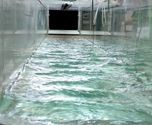
  $x$, as is presented schematically in figure 1(a); variation of wave parameters with fetch is clearly visible in figure 1(b). It is important to note that the simplified two-dimensional illustration in figure 1(a) does not fully depict real wind waves that are essentially random and three-dimensional, as seen in the snapshots. The vertical scale of wind waves may be presented by the characteristic r.m.s. surface elevation $(\overline {\eta (x)^2})^{1/2}$ computed as the time average of the measured variation in time of the surface elevation $\eta (t)$ relative the mean water level.

Figure 1. (a) Schematic illustration of wind waves growth and the developing boundary layer in air; (b) snapshots of the wave field taken through the side window of the test section at three locations; the maximum velocity  $U_0=11.2\ {\rm m}\ {\rm s}^{-1}$.
Velocity profiles were measured at multiple elevations above the mean water surface level at seven fetches in the range  $1\ {\rm m}\leqslant x \leqslant 3.4\ {\rm m}$ and at six wind velocities. The mean wind velocities derived from profiles $U(z)$ are listed in table 1. For any given blower setting, the maximum wind velocities $U_0$ remained practically constant along the whole test section. In Zavadsky & Shemer (Reference Zavadsky and Shemer2012), the values of $u_*$ were extracted by two independent methods, from the measured mean turbulent velocity profile in the inner part of the boundary layer above the wavy water surface and from the Reynolds shear stresses. Estimates based on the two approaches agreed well and demonstrated that for a given airflow rate, the variation of $u_*$ with fetch did not exceed approximately 7 %. The mean values of the friction velocities obtained in Zavadsky & Shemer (Reference Zavadsky and Shemer2012) for a given air flow forcing are referred to as $u_{*,ZS}$ in table 1. Additional independent evaluation of $u_*$ was performed based on the boundary layer momentum integral equation, for details see Appendix A. Those values are referred to as $u_{*, MI}$ and mostly agree well with the estimates based on Zavadsky & Shemer (Reference Zavadsky and Shemer2012). The somewhat higher values of $u_{*,ZS}$ may be attributed to an unavoidable overestimate of the friction velocity in the presence of high amplitude waves owing to the insertion of some portion of the wake in the fit. The integral method is more robust and less sensitive to the profile details in the lower part of the boundary layer; it thus indeed yields lower values of $u_*$ at those conditions. In the following, for each $U_0$, the average values of $u_*$ presented in the two columns of table 1 are used.
Table 1. Characteristic mean wind velocities:  $U_0$, the maximum wind velocity; $u_*$, the friction velocity; $U_{10}$, the estimated wind velocity at $z=10\ {\rm m}$ (1.1). Here the subscripts ZS and MI refer to Zavadsky & Shemer (Reference Zavadsky and Shemer2012) and to the momentum integral (Appendix A).

The dimensionless profiles are plotted in figure 2 and compared with the logarithmic velocity profile in turbulent flow over a smooth plate:
 \begin{equation} U^+{=}\frac{U(z)}{u_*}=\frac{1}{\kappa}\ln (z^+)+B, \end{equation}
where  $B=5.1$, and the wall unit $\nu /u_*$ serves as the length scale; $\nu$ is the kinematic viscosity of air; the scaled variables are denoted by ‘ $+$’. The values of $U_{10}$, estimated by extrapolating (1.1) to $z=10\ {\rm m}$, vary with fetch by less than 6 %; the mean values of $U_{10}$ are specified in table 1.

Figure 2. Dimensionless mean velocity profiles at various wind velocities and fetches.
The slopes of the velocity profiles in the logarithmic innermost part of the boundary layers (Zavadsky & Shemer Reference Zavadsky and Shemer2012) are very close to that of the smooth solid surface. It is evident that at each fetch, the profiles are shifted down with an increase in wind velocity. A similar downshift of profiles with  $u_*$ was observed in the detailed PIV measurements performed by Buckley et al. (Reference Buckley, Veron and Yousefi2020) at a significantly larger fetch ( $x=22.7\ {\rm m}$). For a given friction velocity $u_*$, the downshift of profiles with fetch is observed in this figure. This finding indicates that for young wind waves, the value of the Charnock constant in (1.2) varies with $x$. It thus seems appropriate to apply an alternative to the (1.1) approach to describe the shape of the turbulent velocity profiles over wind waves that is based on the directly measured quantities.
The vertical shift in the velocity profiles, as presented in figure 2, was treated for solid rough surface by Clauser (Reference Clauser1954) and Hama (Reference Hama1954) who modified the smooth velocity profile (3.1) to
 \begin{equation} U^+(z^+)=\frac{1}{\kappa}\ln(z^+)+B-\Delta U^+, \end{equation}
where the amount of the downshift  $\Delta U^+$ depends on the dimensionless characteristic roughness height $k_s^+$. Hudson, Dykhno & Hanratty (Reference Hudson, Dykhno and Hanratty1996) measured the statistical characteristics of the turbulent boundary layer over a solid wavy surface and suggested using the wave height as the appropriate vertical roughness scale. Inspired by this approach, the local dimensionless surface roughness of random wind waves that evolve with fetch is parametrized here by the local characteristic r.m.s. values of the surface elevation $k_s^+=\eta _{rms}^+= (\overline {\eta (x)^2})^{1/2}u_*/\nu$. It should be stressed that drift current at the water surface induced mainly by wind shear exists and is estimated as $0.2u_*< u_s<0.5u_*$ (Toba Reference Toba1988; Tseng et al. Reference Tseng, Hsu and Wu1992; Caulliez et al. Reference Caulliez, Makin and Kudryavtsev2008; Zavadsky & Shemer Reference Zavadsky and Shemer2017b). This drift, however, does not affect the outcome notably because $\Delta U^+$ represents the difference in velocities over the smooth and wave water surfaces, so that the contribution of $u_s$ is cancelled.
The validity of this parametrization is examined in figure 3 where the dimensionless downshift  $\Delta U^+$ is plotted as a function of the local $\eta _{rms}^+$. The coloured markers denote the dimensionless downshift $\Delta U^+$ estimated from the velocity profiles, see figure 2, the black symbols represent estimates of $\Delta U^+$ made on the basis of the alternative published data.The broken line corresponds to the roughness functions $\Delta U^+(\eta _{rms}^+)$ given by
 \begin{equation} \Delta U^+{=}\frac{1}{\kappa}\ln(\eta_{rms}^+)+B-B_{RF}, \end{equation}
with  $B_{RF}$ defined by Nikuradse (Reference Nikuradse1950). The roughness function $\Delta U^+$ in the fully rough regime corresponds to $B_{RF}=8.5$ and is plotted by a solid line.

Figure 3. Hama roughness function  $\Delta U^+(\overline {\eta ^2}^{1/2}u_*/\nu )$. Colours and markers as in figure 2.
Nikuradse estimated that for monodisperse close-packed sand grain roughness, the onset of the fully rough regime occurs at  $k_s^+\approx 70$. However, the roughness type and uniformity may advance the onset of a fully rough boundary layer, see Schultz & Flack (Reference Schultz and Flack2007) and references therein. As documented by Liberzon & Shemer (Reference Liberzon and Shemer2011), Zavadsky & Shemer (Reference Zavadsky and Shemer2017a) and Shemer et al. (Reference Shemer, Singh and Chernyshova2020), the characteristic water surface roughness $\eta _{rms}$ increases with the fetch $x$ for a constant friction velocity $u_*$, and with $u_*$ for a constant fetch. Figure 3 demonstrates that the downward shift $\Delta {U^+}$ increases with the scaled surface roughness $\eta _{rms}^+$ and follows the expected fully rough asymptote for majority of cases examined here.
The results obtained at diverse wind velocities and fetches in three different facilities thus correspond fairly well to fully rough conditions with  $\eta _{rms}$ serving as the characteristic roughness. Therefore, the fully rough velocity profile over wind-generated waves at each fetch $x$ in all those cases can be presented as
 \begin{equation} U^+(x,z)=\frac{1}{\kappa}\ln\left(\frac{z}{\eta_{rms}(x)}\right)+8.5. \end{equation}
 It is evident from (3.4) that the shapes of the mean velocity profile in the overlap region are unaffected by the roughness  $\eta _{rms}$, which determines only their vertical shift. This wall similarity directly relates the shape of the velocity profile to the local characteristic wave height.
Comparison of (3.4) and (1.1) allows for relating the roughness parameter  $z_0$ to the directly measurable characteristic surface elevation variation, yielding for a fully rough surface $\eta _{rms}\approx 30z_0$ that can be measured relatively easily. It is thus preferable to use (3.4) to characterize the shape of the velocity profile in air over wind waves. In particular, (3.4) enables determination of the commonly adopted characteristic wind velocity estimated at $z=10\ {\rm m}$ over the water surface, $U_{10}$.
Additional insight into interaction of wind and waves may be gained by analysing the integral boundary layer parameters based on the measured velocity profiles. The variation of the estimated values of the boundary layer thickness  $\delta$, the displacement thickness $\delta _1=\int _0^\delta (1-U(z)/U_0) \,{\rm d}z$ and the momentum thickness $\delta _2=\int _0^\delta (U(z)/U_0) (1-U(z)/U_0) \,{\rm d}z$ with fetch $x$ are plotted in figure 4(a–c) for the wind velocities given in table 1. Note that to calculate $\delta _1$ and $\delta _2$, the lower part of the velocity profile adjacent to the interface was approximated using the lin-log velocity profile suggested by Miles (Reference Miles1957) that smoothly connects the linear viscous sublayer to the logarithmic overlap region.

Figure 4. Boundary layer characteristics: (a) boundary layer thickness; (b) displacement thickness; (c) momentum thickness; (d) ratio of boundary thickness and roughness height  $a=\sqrt 2\eta _{rms}$; (e) vertical profile of normalized Reynolds stress; ( f) velocity defect profiles using mixed outer scale at all conditions in figure 2. Colours in panels (a–d) and symbols in panels (e, f) as in figure 2.
Jimenez (Reference Jimenez2004) asserted that wall similarity holds once the roughness height  $k$ is sufficiently small, so that $\delta /k>40$. The relative height of the roughness manifested by the ratio of the boundary layer thickness and the characteristic wave amplitude $\delta /a$, where $a=\sqrt 2 \eta _{rms}$, decreases with wind velocity, see figure 4(d). The values of $\delta /a$ are below the limit of Jimenez (Reference Jimenez2004). Nevertheless, as demonstrated in figure 3, wall similarity is maintained in all those cases. This finding supports the applicability of a lower critical value of $\delta /k=5$ suggested by Castro (Reference Castro2007).
The dimensionless velocity defect values  $U_0^+-U^+$ measured in our facility at multiple fetches and wind velocities presented in figure 2 are plotted in figure 4(e). The values of $u_*$ given in table 1 are used for normalization. It is evident that in this representation, all velocity profiles collapse. The roughness effects that may destruct the near-wall coherent structures are thus confined to the inner layer, i.e. the innermost part of the boundary layer. This feature of the velocity profiles implies wall similarity (Raupach, Antonia & Rajagopalan Reference Raupach, Antonia and Rajagopalan1991). The distributions of the normalized Reynolds shear stress $-\overline {u'w'}^+$ plotted for those conditions in figure 4( f) also collapse. The scatter in figure 4(e–f) may be attributed to variations of the friction velocity $u_*$ with fetch that are estimated at approximately 7 %. Figure 4(e–f) thus provide additional evidence for the existence of wall similarity of the overlap and outer layers over young wind waves.
The airflow in the test section is maintained by a favourable pressure gradient. Boundary layer similarity in the presence of the pressure gradient requires that the Clauser parameter remains constant (White Reference White2006):
 \begin{equation} \beta=\frac{\delta_1}{\tau}\frac{{\rm d}p}{{\rm d} x}. \end{equation}
The values of  $\beta$ evaluated for the present experimental conditions based on direct pressure drop measurements presented in Liberzon & Shemer (Reference Liberzon and Shemer2011), and on the displacement thickness presented in figure 4(b), yield $\beta$ that do not change significantly and remain in the range from $-0.17$ to $-0.1$. Note that the slope of the dimensionless Reynolds stress with the dimensionless vertical coordinate, presented by a dashed line in figure 4( f), equals to $-1$, allowing independent evaluation of the Clauser parameter as
 \begin{equation} \beta={-}\frac{\delta_1}{\delta}\frac{\partial(\overline{u'w'}^+)}{\partial (z/\delta) }\approx{-}\frac{\delta_1}{\delta} \end{equation}
that is consistent with (3.5), see figure 4(a,b). To further support the equilibrium boundary layer defined by Clauser, the values of the defect shape factor, defined as
 \begin{equation} G=\frac{u_*}{\delta_1U_0}\int_0^\delta \left(\frac{U_0-U(z)}{u_*}\right)^2 \,{\rm d}z, \end{equation}
were calculated and are presented in table 2. Nearly constant values of  $G$ in this table provide further support for invariance of the velocity defect profile (Mellor & Gibson Reference Mellor and Gibson1966).
Table 2. Values of defect shape factor  $G$ computed by (3.7) for all fetches and wind forcing. The r.m.s. of the data is 5.13 with a standard deviation of 0.33.

4. Drag coefficients over wind waves
The friction at the water surface is commonly quantified in wind wave modelling and meteorology studies using  $U_{10}$ that serves as the velocity scale. Following Donelan (Reference Donelan1998) and Donelan et al. (Reference Donelan, Haus, Reul, Plant, Stiassnie, Graber, Brown and Saltzman2004), the corresponding drag coefficient is defined as $C_D=(u_*/U_{10})^2$. The results of Donelan et al. (Reference Donelan, Haus, Reul, Plant, Stiassnie, Graber, Brown and Saltzman2004) plotted in figure 5(a) agree reasonably well with those derived from the laboratory measurements (Mitsuyasu Reference Mitsuyasu1970; Mitsuyasu & Honda Reference Mitsuyasu and Honda1974, Reference Mitsuyasu and Honda1982; Caulliez et al. Reference Caulliez, Makin and Kudryavtsev2008; Buckley et al. Reference Buckley, Veron and Yousefi2020) and the values of $C_D$ derived from the data presented in table 1. The field results of Mitsuyasu (Reference Mitsuyasu1969) are included in this figure as well. The plotted values of $C_D$ were estimated using the values of $u_*$ and $U_{10}$ reported in those references.


Note that the results of Donelan et al. (Reference Donelan, Haus, Reul, Plant, Stiassnie, Graber, Brown and Saltzman2004) indicate that the saturation of  $C_D$ is attained at wind velocities $U_{10}$ exceeding approximately $40\ {\rm m}\ {\rm s}^{-1}$. Wu (Reference Wu1969) observed similar saturation at $U_{10} > 15\ {\rm m}\ {\rm s}^{-1}$; he attributed it to the fact that at those conditions, the water surface becomes fully rough with $k_s^+$ based on the Nikuradze sand grain height exceeding 70. The present results, however, demonstrate that the velocity downward shift follows the fully rough asymptote even at notably lower wind velocities. Thus, the water surface may become effectively fully rough, while the friction coefficient $C_D$ is still well below its saturation level.
The effect of the surface roughness, manifested in the vertical displacement of similar velocity profiles as compared to the smooth-wall case, results in a momentum deficit related to the momentum exchange between airflow and waves. The skin-friction factor, defined as  $c_f=2(u_*/U_0)^2$, is related to the momentum deficit. The integral momentum equation in the presence of pressure gradient applied in Appendix B to relate $c_f$ to $x/k_s$. Figure 6 in this appendix demonstrates that for the Clauser parameters encountered in the present study, the resulting relation does not differ notably from that obtained for a fully rough turbulent boundary layer over a surface with a constant roughness $k_s$ in the absence of a pressure gradient (Prandtl & Schlichting Reference Prandtl and Schlichting1934; Schlichting Reference Schlichting1979) :
 \begin{equation} c_f=[2.87+1.58 \log_{10}(x/k_s)]^{{-}2.5}. \end{equation}
Figure 6. (a) Surface elevation as a function of  $x$ for various wind velocities: solid lines, linear fits; dashed lines, numerical solution of (B9). (b) Skin-friction coefficient dependence on dimensional fetch; solid line corresponding to (4.1) for rough flow with no pressure gradient is plotted for comparison. Coloured markers, the mean values of $c_f$ presented in table 1 as a function of the values of $x/\eta _{rms}$ estimated from figure 6(a).
The skin friction is the governing parameter that couples the airflow with water waves and shear current. The values of  $c_f$ evaluated using (4.1) that relate the data on airflow and water-wave measurements acquired in various studies are presented in figure 5(b). To compare results of multiple studies on wind waves, the dimensionless customary adopted fetch $\hat {x}=xg/u_*^2$ is used. All studies show that the increase in $\hat {x}$ results in a decrease of $c_f$. In the inset to figure 5(b), the values of $c_f$ from (4.1) are compared with $2(u_*/U_0)^2$ showing reasonable agreement. Note that although constant roughness is assumed in derivation of (4.1), the fetch-dependent effective roughness $\eta _{rms}(x)$ is used. The applicability of (4.1) supports the conjecture that the turbulent boundary layer in airflow over young water waves indeed satisfies wall similarity over a rough wavy water surface. The inset indicates that for each $U_0$, the values of $c_f$ practically do not depend on the fetch, as observed in fully rough flows over a solid surface with $k_s\sim x$. As demonstrated in Appendix B, in the present experiments, the characteristic amplitude of the young wind waves $\eta _{rms}$ in fact increases approximately linearly with $x$ for each wind velocity $U_0$.
While the majority of the available results were obtained in laboratory facilities, results of field measurements reported by Mitsuyasu (Reference Mitsuyasu1969) were also included in figure 5(b) and allowed to extend the range of dimensionless fetches  $\hat {x}$ to six orders of magnitude. The fully rough estimates are based on the reported values of the fetch $x$ and $\eta _{rms}$, while the smooth surface values correspond to the flow over a flat plate at high Reynolds numbers (Schlichting Reference Schlichting1979). It should be stressed that the wave steepness in laboratory experiments is usually significantly higher than that in field studies. The characteristic wave steepness measured directly by Zavadsky & Shemer (Reference Zavadsky and Shemer2017a) using a laser slope gauge does not vary significantly with fetch, in spite of wave amplitude growth. For all wind velocities applied in their experiments, the measured values of the characteristic steepness remain close to $\epsilon = 0.2$. Similar values of the measured steepness were reported by Hsu et al. (Reference Hsu, Wu, Hsu and Street1982) and Buckley et al. (Reference Buckley, Veron and Yousefi2020). Buckley et al. (Reference Buckley, Veron and Yousefi2020) demonstrated that at those values of $\epsilon$, the total skin friction is mostly determined by the form drag, whereas the contribution of the viscous drag is relatively minor. This observation is consistent with the statement by Flack & Schultz (Reference Flack and Schultz2014) that a fully rough regime is characterized by the dominant contribution of the form drag of the roughness elements. Moreover, according to Buckley et al. (Reference Buckley, Veron and Yousefi2020), for $\epsilon \approx 0.2$, the entire wind stress is transferred to the wave motion, whereas at $\epsilon <$0.1, less than 50 % is transmitted. In the field experiments of Mitsuyasu (Reference Mitsuyasu1969), the estimated wave steepness is $\epsilon \approx 0.05$. It can be seen from figure 5(b) that both rough and smooth surface estimates of $c_f$ yield results of the same order of magnitude. Note that extrapolation of the experimentally estimated values of $c_f$ to higher dimensionless fetches, attempted by a broken line in figure 5(b), suggests that the friction factors may fall within these extreme values. Although the wave ages $c_p/u_*$ for the flow conditions in figure 2 do not exceed unity, the results presented in figure 5(b) may be applicable also for faster moving longer waves.
5. Discussion and conclusions
Coupling between airflow and water waves is studied here on the basis of extensive experimental data on velocity profiles in air over wind waves at different wind velocities and fetches accumulated in our wind wave tank. The wind velocity information is associated with the corresponding data on the characteristic parameters of wind waves. When possible, analysis is supported by data extracted from additional laboratory studies, as well as from reports on field measurements. We also take advantage of the considerable progress made in recent decades in the analysis of turbulent flows over solid rough surfaces where the wall similarity of turbulent boundary layer has been studied in detail for a variety of geometric parameters. We apply this approach to air flow over the perpetually moving wavy water surface.
The moving three-dimensional random water surface is characterized by a wide spectrum of wavelengths that may evolve in time as well as in space. It is thus considerably more complicated than the ‘frozen’ rough solid surface that, in most studies, is assumed as spatially homogeneous. The airflow over wind waves differs from that over a solid surface in several important aspects. The dynamic coupling between the airflow and wind waves results in a transfer of energy and momentum from wind to the water surface causing wind wave growth; this effect does not exist in the case of a rigid surface. In measurements of a solid rough surface, the vertical distance from the surface at the sensor location remains fixed, whereas in water wave experiments, the elevation of the sensor over the instantaneous surface level varies continuously. Special effort was therefore invested by Zavadsky & Shemer (Reference Zavadsky and Shemer2012) in the determination of the mean surface elevation at each fetch and wind forcing conditions that may be different from the still surface level; the mean wind velocity profiles were obtained relative to this reference height. The movement of the interface becomes even more essential in the determination of the turbulent parameters of the airflow above the water surface. There seems to be no straightforward way to decouple the velocity fluctuations that are intrinsic to the turbulent airflow, from variations related to the random water surface movement. First, as mentioned above, the elevation of the sensor relative to the instantaneous local surface position varies in time and may cause fluctuations in the measured velocity. Second, the wavy motion observed in water also exists in air. The corresponding airflow orbital velocities have a wide spectrum related to the spectrum of the surface elevation in the presence of wind waves; the phases of those fluctuations are random. The fluctuations associated with waves in airflow decay exponentially with height above the mean surface. These two phenomena result in the characteristic fluctuations of the horizontal,  $\overline {u'^2}^{1/2}$, and vertical, $\overline {w'^2}^{1/2}$, velocity components, that at low elevations are notably higher than the corresponding values measured in boundary layers over smooth and rough surfaces (Zavadsky & Shemer Reference Zavadsky and Shemer2012). An additional but less important complication is related to the drift current induced by wind shear as well as by the water waves’ nonlinearity.
Probably for those reasons, the structure of the turbulent boundary layer over wind waves so far has not been related directly to their characteristics. The roughness parameter  $z_0$ that was introduced empirically to describe the wind velocity profile over waves cannot be easily related to water surface properties. We suggest using the measurable characteristic wave amplitude $\eta _{rms}$ as an analogue to the roughness $k_s$ that characterizes flows over rough surfaces. Laboratory-scale experiments necessarily study the so-called ‘young’ wind waves characterized by wave steepness that often exceeds that commonly encountered in the open sea. The water surface in the presence of young wind waves is thus effectively fully rough. Although under steady wind forcing the wave height increases with fetch, the characteristic steepness remains essentially unchanged along the test section. In this sense, the water surface in a wind wave tank retains approximately similar geometry. Note that experiments show that the friction velocity $u_*$ also does not vary significantly with $x$ for a constant wind velocity $U_0$.
In the current study, we have demonstrated the existence of wall similarity in the spatially developing boundary layer over wind waves. The invariance of the velocity-defect profiles in figure 4(e, f) implies that the direct influence of the local water surface roughness  $k_s=\eta _{rms}(x)$ is confined to the inner part of the boundary layer. The downward shift of the velocity profiles $\Delta U^+$ corresponds to the rise in momentum deficit that is directly related to increase in frictional drag. It was found that when the roughness is taken as $k_s=\eta _{rms}$, $\Delta U^+$ follows the fully rough asymptote. This implies that for young wind wave studies, the wall shear stress is almost entirely owing to form drag, in agreement with Buckley et al. (Reference Buckley, Veron and Yousefi2020). It should be stressed that the onset of a fully rough regime in flow over wind waves occurs at roughness $\eta ^+_{rms}$ that is considerably below Nikuradse's criterion $k_s^+>$70. This may be attributed to a difference in the roughness type. Under all experimental conditions in our facility, wall similarity was found up to $\delta /a\approx 5$, where the characteristic wave amplitude is defined as $a=\sqrt 2\eta _{rms}$, in agreement with the limit over a solid surface found by Castro (Reference Castro2007).
The coupling between airflow and water surface is characterized by the drag coefficients. The values of  $C_D$ in our experiments agree well with data available elsewhere, see figure 5(a). Definition of $C_D$ based on a wind velocity characterized by $U_{10}$ is physically irrelevant in a laboratory facility; it is thus more sensible to use the maximum wind velocity $U_0$ that defines the skin-friction coefficient $c_f=2(u_*/U_0)^2$ that is related to the derivative of the momentum thickness, (A2). Fully rough flows over solid surfaces are dominated by pressure drag, the momentum integral combined with the rough wall-velocity profile leads to a relation $c_f =f(x/k_s)$ that agrees well with (4.1), see Appendix B. For fully rough conditions in our wind wave experiments, this relation is applicable under various wind velocities and agrees with the constant with an $x$ estimate of $2(u_*/U_0)^2$, figure 5(b). Similar to fully rough regime over solid surfaces, constant $c_f$ in a developing boundary layer is possible only when $x/k_s$ remains constant (Chung et al. Reference Chung, Hutchins, Schultz and Flack2021). This occurs when the vertical and horizontal scales of the roughness grow linearly along the plate (Talluru et al. Reference Talluru, Djenidi, Kamruzzaman and Antonia2016; Sridhar, Pullin & Cheng Reference Sridhar, Pullin and Cheng2017). We have shown that $c_f$ obtained at the interface of the wavy water surface depends entirely on $x/\eta _{rms}(x)$ and indeed does not vary notably. To the best of our knowledge, this finding has not yet been reported in boundary layers over wind waves. Because $c_f$ depends merely on the local surface elevation, the shear stress responsible for the momentum flux into the wave field can be evaluated as well.
Funding
This study was supported by grant 508/19 from Israel Science Foundation. Partial support to M.G. by Ben Gurion University is gratefully acknowledged.
Declaration of interests
The authors report no conflict of interest.
Appendix A. An evaluation of the friction velocity using momentum integral equation
Friction velocities can be estimated independently using the momentum integral equation that, in the presence of a pressure gradient, can be written as
 \begin{equation} \frac{u_*^2}{U_0^2}=\frac{{\rm d}\delta _2}{{\rm d} x}-(2\delta _2+\delta _1)\frac{1}{\rho U_0^2}\frac{{\rm d}p}{{\rm d} x} . \end{equation}
Here  $\delta$, $\delta _1$ and $\delta _2$ are the boundary layer thickness, the displacement thickness and the momentum thickness, respectively. Because $-\partial (\overline {u'w'}^+)/\partial (z/\delta )\approx -1$ (figure 4f), substituting (3.5) and (3.6) into (A1) results in
 \begin{equation} \frac{u_*^2}{U_0^2}\approx\frac{{\rm d}\delta _2}{{\rm d} x}+\frac{(2\delta _2+\delta _1)}{\delta}\frac{u_*^2}{U_0^2} . \end{equation}
Rearranging (A2) yields a simple approximation for  $u_*$,
 \begin{equation} u_*=U_0\sqrt{\left.\frac{{\rm d}\delta _2}{{\rm d} x}\right/\left(1-\frac{2\delta _2+\delta _1}{\delta}\right)} . \end{equation}
Estimates of  $\delta$, $\delta _1$ and $\delta _2$ presented in figure 4(a–c) allow therefore to obtain the values of $u_*$ for all wind forcing conditions at six fetches; the results are listed in table 3.
Table 3. Values of friction velocity in  ${\rm m}\ {\rm s}^{-1}$ computed by (A3) for data in figure 4(a–c).

Table 3 shows that for the given wind velocity  $U_0$, the values of $u_*$ remain nearly constant along the test section, in agreement with the available laboratory studies (Mitsuyasu & Rikiishi Reference Mitsuyasu and Rikiishi1978; Hsu et al. Reference Hsu, Wu, Hsu and Street1982; Caulliez et al. Reference Caulliez, Makin and Kudryavtsev2008; Zavadsky & Shemer Reference Zavadsky and Shemer2012). For lower wind velocities, $U_0 \leqslant 8.9\ {\rm m}\ {\rm s}^{-1}$, the average values of $u_*$ agree well with the friction velocities in table 1. For the two higher wind velocities, estimates based on the momentum integral yield values approximately $10\,\%$ smaller than those derived from the velocity profile fit, see table 1. Owing to inherent difficulties in the measurements of airflow close to the interface in the presence of large random wind waves under those wind forcing conditions, for $U_0=10.05$ and $11.2 {\rm m}\ {\rm s}^{-1}$, Zavadsky & Shemer (Reference Zavadsky and Shemer2012) extended the fitting domain up to $z/\delta <0.3$ instead of $z/\delta < 0.2$ applied for lower wind velocities. This extension to the outer part of the boundary layer apparently caused incorporation in the fitting domain of a small portion of the wake region, which resulted in overestimate of the friction velocities. Nevertheless, application of the integral momentum method, which is less sensitive to the inner region, shows that the resulting error is relatively small and comparable with the experimental uncertainty. The average value of $u_*$ was computed for each wind velocity $U_0$; the corresponding averages denoted as $u_{*,MI}$ are listed in table 1. All values of $u_*$ presented in table 1 agree well with Plant & Wright (Reference Plant and Wright1977). The use of the momentum integral (A1) thus provides reasonably accurate prediction of the friction velocity in air flow over young wind waves at all wind forcing conditions.
Appendix B. Estimates of  $c_f=f(x/k_s,\varPi )$ based on the momentum integral equation

The integral momentum equation approach applied by Prandtl & Schlichting (Reference Prandtl and Schlichting1934) and Schlichting (Reference Schlichting1979) to derive the skin-friction coefficient dependence on fetch  $c_f=f(x/k_s)$ for airflow above a fully rough surface is extended here to account for the presence of a pressure gradient and the fetch dependence of roughness $k_s$. The velocity profile in the overlap and in the outer layers of fully rough flows can be presented as
 \begin{equation} U^+(z)=\frac{1}{\kappa}\ln\left(\frac{z}{k_s}\right)+B_{RF}+\frac{2\varPi}{\kappa}\sin^2\left(\frac{{\rm \pi} z}{2\delta}\right) . \end{equation}
Here  $B_{RF}=8.5$ and $\varPi$ is the Cole's wake parameter that depends on the Clauser's pressure parameter $\beta$ only (White Reference White2006). At the edge of the boundary layer $z=\delta$,
 \begin{equation} U_0^+{=}\sqrt{\frac{2}{c_f}}=\frac{1}{\kappa}\ln\left(\frac{\delta}{k_s}\right)+B_{RF}+\frac{2\varPi}{\kappa} . \end{equation}
The ratio of the boundary layer thickness and the equivalent sand grain roughness is thus
 \begin{equation} \frac{\delta}{k_s}=\exp\left({\kappa\left(U_0^+{-}B_{RF}-\frac{2\varPi}{\kappa}\right)}\right). \end{equation}
The displacement thickness  $\delta _1$ and the momentum thickness $\delta _2$ for the velocity profile given by (B1) are (Sridhar et al. Reference Sridhar, Pullin and Cheng2017)
 $$\begin{gather} \delta_1=\delta \dfrac{1+\varPi}{\kappa B_{RF} +2\varPi+\ln \dfrac{\delta}{k_s}}, \end{gather}$$
 $$\begin{gather}\delta_2=\delta \dfrac{\varPi^2-4+2\kappa B_{RF}(1+\varPi)+2(1+\varPi)\ln \dfrac{\delta}{k_s}-4\varPi Q/{\rm \pi}}{2\left(\kappa B_{RF} +2\varPi+\ln \dfrac{\delta}{k_s}\right)^2} . \end{gather}$$
Here,  $Q=\int _{0}^{{\rm \pi} } \sin (z)/z \,{\rm d}z=1.85$. It follows from (B2) and (B4) that
 $$\begin{gather} \delta_1=\delta\frac{1+\varPi}{\kappa U_0^+}, \end{gather}$$
 $$\begin{gather}\delta_2=\delta\left[\frac{\varPi^2-4-4\varPi(1+\varPi)-4\varPi Q/{\rm \pi}}{2\left(\kappa U_0^+\right)^2} +\frac{1+\varPi}{\kappa U_0^+}\right]=\delta G(U_0^+,\varPi) . \end{gather}$$
Because  $\delta _1/\delta$ and $\delta _2/\delta$ depend on $U_0^+$ and $\varPi$, (A2) can be rearranged as
 \begin{equation} \frac{{\rm d}\delta_2}{{\rm d}x}=\frac{1}{U_0^+}\left(1-\frac{2\delta_2+\delta_1}{\delta}\right)=F(U_0^+,\varPi) \end{equation}
 \begin{equation} \frac{{\rm d}\delta_2}{{\rm d} x}=G\frac{{\rm d}\delta}{{\rm d} x}+\delta\frac{\partial G}{\partial U_0^+}\frac{{\rm d}U_0^+}{{\rm d} x}+\delta \frac{\partial G}{\partial \varPi}\frac{{\rm d}\varPi}{{\rm d} x}=F . \end{equation}
In the present study, this relation is simplified because  ${\rm d}U_0^+/{{\rm d} x}=0$,
 \begin{equation} \frac{{\rm d}\delta}{{\rm d} x}=\frac{F-\delta \dfrac{\partial G}{\partial \varPi}\dfrac{{\rm d}\varPi}{{\rm d} x}}{G} . \end{equation}
For a given  $\varPi (x)$ and $U_0^+$, this relation can be solved by a numerical integration procedure resulting in $\delta =\varPhi (x)$ leading to a relation for $k_s(x)$ based on (B3),
 \begin{equation} k_s=\frac{\varPhi(x)}{\exp({\kappa(U_0^+{-}B_{RF}-2\varPi(x)/\kappa)})}. \end{equation}
 Fitting the velocity distributions in figure 2 to (B1) leads to the Coles’ parameter estimates as  $\varPi \approx 0.1x$. This dependence was substituted in (B8) and for a given $U_0^+$, this equation was integrated by a fourth-order Runge–Kutta integration routine with initial value of $\delta \approx 0.05\ {\rm m}$ at $x=1\ {\rm m}$. The variations of $k_s$ with downstream distance $x$ were computed using (B9) and plotted in figure 6(a) by dashed lines; the experimental results are plotted in this figure as well. Linear fits were also added to the scatter at each wind forcing (solid lines). At each wind velocity $U_0$, the results exhibit a reasonably accurate linear fit, with the scatter that increases somewhat for the highest wind velocity. Talluru et al. (Reference Talluru, Djenidi, Kamruzzaman and Antonia2016) and Sridhar et al. (Reference Sridhar, Pullin and Cheng2017) showed that in boundary layers over a rough solid surface, $c_f$ remains constant when the roughness varies linearly with $x$. This condition is satisfied reasonably well for the present experiments. The approximately linear with $x$ growth of the water surface roughness represented by $\eta _{rms}$ enables estimation of the values of $x/\eta _{rms}= x/k_s$ based on the fit slopes (table 4). The values of $c_f=2u_*^2/U_0^{2}$ in this table are evaluated using the friction velocities listed in table 1 and were plotted versus $x/\eta _{rms}$ with the corresponding error bars (figure 6b). The solid line corresponds to the case of the turbulent flow over a surface with a constant roughness in the absence of a pressure gradient (4.1) and agrees fairly well with the present results. The curve in figure 6(b) allows for a reasonably accurate estimate of the characteristic surface elevation for young wind waves in any fetch for a given $u_*/U_0$. It should be stressed that the effect of a small favourable pressure in the present experiments ( $\beta <0.2$) is practically negligible.
Table 4. Experimental values of  $x/\eta _{rms}$ obtained as inverse of slopes in figure 6(a) and skin friction coefficients using $u_*$ values specified in table 1. Here, subscript ZS refers to Zavadsky & Shemer (Reference Zavadsky and Shemer2012) and MI refers to the momentum integral equation.


 Open access