


1. Introduction
The squeeze-induced flow of thin films is found in many engineering and natural systems. Such cases include hydrodynamic load and thrust bearings (Venerus Reference Venerus2018), hydraulic fractures (Holditch Reference Holditch2007), diarthrodial joints (e.g. knee and hip, Knox et al. Reference Knox, Wilson, Duffy and McKee2015; Karmakar & Raja-Sekhar Reference Karmakar and Raja-Sekhar2018), soft robotics (Matia & Gat Reference Matia and Gat2015) and various microfluidic applications (Christov et al. Reference Christov, Cognet, Shidhore and Stone2018; Wang & Christov Reference Wang and Christov2019). However, many such applications involve not only a pressure-driven or boundary-driven motion along the channel, but can involve permeation into either a rigid or compressible porous layer. For example, hydraulic fracturing processes are typically characterized by the fluid–structure interaction with a low-permeability rock layer and in some cases the interaction of discrete fractures with high-volume natural faults or higher-permeability layers (Pritchard, Woods & Hogg Reference Pritchard, Woods and Hogg2001; Brownlow, James & Yelderman Reference Brownlow, James and Yelderman2016; Ray Reference Ray2017).
In many of the cases mentioned above, common applications (such as microfluidic devices, e.g. Pranzo et al. Reference Pranzo, Larizza, Filippini and Percoco2018) or their physical description in complex natural systems (such as joints or fracture systems, e.g. Wei & Xia Reference Wei and Xia2017) involve a network-like structure in which flow occurs between regions with varying dimensions or mechanical properties. Invariably, modelling physical mechanisms such as elastic deformation or leakage in such spatially varying dynamical systems typically comes at the expense of their spatial complexity (Inamdar, Wang & Christov Reference Inamdar, Wang and Christov2020).
In previous papers we studied the squeeze-induced drainage dynamics for model networks with spatially uniform properties (Dana et al. Reference Dana, Zheng, Peng, Stone, Huppert and Ramon2018), and later, power-law varying properties (Dana et al. Reference Dana, Peng, Stone, Huppert and Ramon2019). In this model, each fluid-filled channel was bounded by two thin rigid plates pressed together in elastic response to a pre-strained state. In this paper, we extend the model to account for the effects of a permeable boundary.
The flow in a single channel of the network is similar to other problems that have been treated previously. For example, the hydrodynamic interaction between a permeable wall and a solid particle (including the case of a variable shape factor) was discussed by Ramon & Hoek (Reference Ramon and Hoek2012) and Ramon et al. (Reference Ramon, Huppert, Lister and Stone2013). The limit where the wall is rigid and the particle has a flat front is analogous to the problem presented here. Venerus (Reference Venerus2018), Karmakar & Raja-Sekhar (Reference Karmakar and Raja-Sekhar2018) and Knox et al. (Reference Knox, Wilson, Duffy and McKee2015, Reference Knox, Duffy, McKee and Wilson2017) investigated squeeze flows in liquid films in a confined channel bounded by a porous disk in contact with either a uniform-pressure reservoir or a sealed edge. However, they all considered the case of a constant load driving the flow. Also, Ray (Reference Ray2017) studied the effect of multiple discrete sinks on leakage rates in a porous medium in a Hele-Shaw cell, and problems describing a single hydraulic fracture propagating in a permeable solid along with the dynamics of fluid withdrawal from a poroelastic layer (in a single fracture) have been discussed previously by Detournay & Garagash (Reference Detournay and Garagash2003) and Marck & Detournay (Reference Marck and Detournay2013).
Herein, following Dana et al. (Reference Dana, Zheng, Peng, Stone, Huppert and Ramon2018, Reference Dana, Peng, Stone, Huppert and Ramon2019), we use a model of an elastic medium to study the effect of leakage on increasingly complicated branching systems. This model is commonly used for a shallow constant-pressure reservoir, a large cavity or a low-pressure high-permeability layer in contact with a thin low-permeability surface, see e.g. Ray (Reference Ray2017), Venerus (Reference Venerus2018) and Pritchard et al. (Reference Pritchard, Woods and Hogg2001).
The paper is structured as follows. In § 2 we formulate the model for a network of fractures with permeable boundaries and provide an appropriate non-dimensionalization. In § 3 we study a single channel and investigate the limits in which drainage is dominated either by parallel flow (towards the outlet) or cross-flow (through the upper boundary). In § 4 we present solutions for a network. Finally, in § 5 we discuss the results and their implications and in § 6 we summarize the main conclusions.
2. Backflow from a permeable network
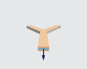
Backflow refers to the reversed flow or fluid drainage from a system due to the relaxation from an initially pressurized state. In the current work, the problem formulation remains similar to that in Dana et al. (Reference Dana, Zheng, Peng, Stone, Huppert and Ramon2018) with modified boundary conditions. Consider a network as a hierarchical structure originating from a single channel located at  $x=0$. This channel is referred to as the outlet channel, as shown in figure 1. The outlet is the furthest downstream point and the pressure there (for studies of backflow) is set to zero. Upstream, the outlet channel bifurcates into two identical channels, which in turn split identically further upstream. The complete set of channels at the same distance, or the number of nodes from the outlet, is referred to as a generation. The network is assumed to have $n$ generations indexed using $i$, with $i=0$ signifying the outlet and $i=n-1$ the furthest upstream channels. The tip end is then the furthest upstream point of the network and flow cannot occur upstream from it (i.e. zero flux at the tip).

Figure 1. A model bifurcating fracture network of  $n$ generations.
2.1. Governing equations
As shown in figure 2, we model the fractures in the network as simple two-dimensional channels bounded by two parallel rigid walls, one of which is permeable, being squeezed together by elastic forces. For simplicity, all fractures have the same constant length  $L$ and initial aperture $h^*=h(0)$. Under the assumption that $h^* \ll L$, we invoke the lubrication approximation for the quasi-steady fluid flow between the plates. We denote $p_i(x,t)$ as the fluid pressure distribution, $h_i(t)$ as the fracture aperture and $\boldsymbol {u}_i(x,y,t)\equiv (u_i,v_i)$ as the velocity field for each fracture in the $i$th generation. Since the plates bounding each channel are rigid, the aperture $h_i(t)$ is solely a function of time. The permeation is assumed to occur against a uniform negligible fluid pressure.
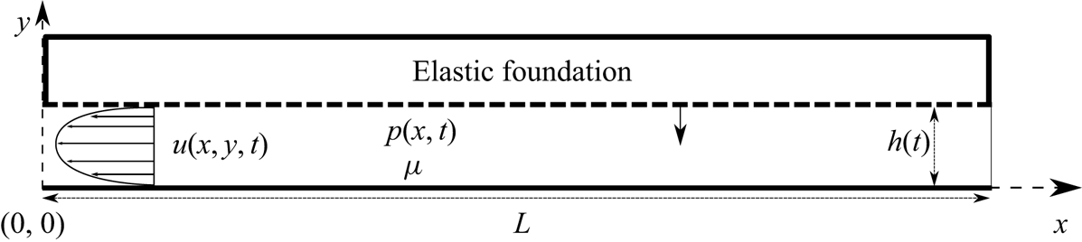
Figure 2. A schematic diagram of a single two-dimensional fracture with a permeable boundary. The fracture is of constant length  $L$ and initial aperture $h^*=h(0)$. For $t>0$ the upper plate is forced down by the elastic response to a pre-strained condition and produces motion of a viscous fluid. When there is no flux at $x=L$, a pressure gradient forms in the $x$ direction and results in an approximately parabolic velocity profile towards the outlet at $x=0$ and permeation along the upper boundary (dashed line) according to (2.2).
The boundary conditions imposed are no slip at both the top and bottom plates, yielding a parabolic velocity profile, leading to the vertically averaged horizontal velocity (Batchelor Reference Batchelor2000, p. 220)
 \begin{equation} \bar{u}_i(x,t)=-\frac{h^2_i(t)}{12\mu}\frac{\partial p_i(x,t)}{\partial x}, \end{equation}
where  $\mu$ is the dynamic viscosity. The bottom plate is impermeable while the permeation through the upper plate into the foundation is assumed to be linearly proportional to the local pressure, resulting in a permeation velocity
 \begin{equation} v_i^p\left[x,h_i\left(t\right),t\right]=\frac{\hat{k}}{\mu}p_i(x,t), \end{equation}
relative to the moving upper plate, where the pressure in the elastic foundation is used as the reference pressure and hence set to zero, and  $\hat {k}$ is the permeability $k$ of the foundation divided by its original (pre-strained) thickness. Thus, (2.2) corresponds to a simplified Darcy's law. Although this model is formulated with permeation only through a single wall, the result (2.4) also applies to permeation through both walls (or, more generally, for any linear coupling between pressure and permeation), provided that the constant $\hat {k}$ is appropriately adjusted.
The cross-channel velocity (measured relative to the stationary, impermeable wall) then satisfies  $v_i=0$ on the lower, impermeable wall, and $v_i=v_i^p+{\textrm {d} h_i(t)}/{\textrm {d} t}$ on the upper, permeable wall. The one-dimensional continuity equation is
 \begin{equation} \frac{\textrm{d} h_i(t)}{\textrm{d} t}+h_i(t)\frac{\partial \bar{u}_i(x,t)}{\partial x}+v_i^p\left[x,h_i(t),t\right]=0. \end{equation}
Substituting the velocity components, (2.1) and (2.2), into the continuity equation (2.3), we obtain the equation for the pressure and aperture, in the form of a modified Reynolds equation,
 \begin{equation} \frac{\textrm{d} h_i(t)}{\textrm{d} t}=\frac{h_i^3(t)}{12\mu}\frac{\partial^2 p_i(x,t)}{\partial x^2}-\frac{\hat{k}}{\mu}p_i(x,t). \end{equation}
The dynamic boundary condition to account for the squeezing force driving the flow was introduced and discussed by Dana et al. (Reference Dana, Zheng, Peng, Stone, Huppert and Ramon2018, Reference Dana, Peng, Stone, Huppert and Ramon2019). For simplicity of notation, we define the position variables
 \begin{equation} x_0=0,\quad x_{i+1}=x_i+L. \end{equation}
The force balance on the upper plate of each generation of the network is written accordingly as
 \begin{equation} \int_{x_i}^{x_{i+1}} p_i(x,t)\,\mathrm{d} x=\hat{E} h_i(t)L, \end{equation}
where  $\hat {E}$, similar to $\hat {k}$, is a modified Young's modulus of the foundation divided by its original thickness.
We require  $n$ initial conditions for $h_i(t)$ and $2n$ boundary conditions for $p_i(x,t)$ (describing zero pressure at the outlet, zero flux at the tip and continuity of pressure and fluid flux at the bifurcating fracture junctions) to complete the problem statement,
 \begin{gather} h_i(0)={{h^*}}, \quad (i=0,1,\dots,n-1), \end{gather}
 \begin{gather}p_0(0,t)=0, \end{gather}
 \begin{gather}p_{i}\left(x_{i+1},t\right)=p_{i+1}\left(x_{i+1},t\right), \quad (i=0,1,\dots,n-2), \end{gather}
 \begin{gather}\left.h_{i}^3 \frac{\partial p_{i}}{\partial x}\right|_{\left(x_{i+1},t\right)}=2h_{i+1}^3 \left.\frac{\partial p_{i+1}}{\partial x}\right|_{\left(x_{i+1},t\right)}, \quad (i=0,1,\dots,n-2), \end{gather}
 \begin{gather}\left.\frac{\partial p_{n-1}}{\partial x}\right|_{(x_n,t)}=0. \end{gather}
The outlet pressure is set to be equal to the reference formation pressure, as any difference between the two pressures is assumed to be small relative to the overpressure in the fracture network.
2.2. Non-dimensionalization
Balancing all terms in (2.4) and (2.6), we define dimensionless variables by
Since this non-dimensionalization involves a balance between lubrication flow and permeation leakage, it is different from that presented in the previous studies of impermeable networks (Dana et al. Reference Dana, Zheng, Peng, Stone, Huppert and Ramon2018, Reference Dana, Peng, Stone, Huppert and Ramon2019). We will use the impermeable scaling, given by (3.3) below, in some comparisons with previous results. The governing equations (2.4) and (2.6) for  $H_i(T)$ and $P_i(X,T)$ then become
 \begin{equation} \frac{\textrm{d} { H}_i}{\textrm{d} T}= H_i^3 \frac{\partial^2 P_i}{\partial X^2}- P_i, \quad \int_{0}^{1} P_i\,\mathrm{d}X=H_i,\quad (i=0,1,\dots,n-1), \end{equation}
and the initial and boundary conditions (2.7) become
 \begin{gather} H_i(0)=H^*, \quad (i=0,1,\dots,n-1), \end{gather}
 \begin{gather}P_0\left(0,T\right)=0, \end{gather}
 \begin{gather}P_i\left(1,T\right)=P_{i+1}(0,T), \quad (i=0,1,\dots,n-2), \end{gather}
 \begin{gather}\left.H_i^3 \frac{\partial P_i}{\partial X}\right|_{\left(1,T\right)}= 2H_{i+1}^3\left. \frac{\partial P_{i+1}}{\partial X}\right|_{\left(0,T\right)}, \quad (i=0,1,\dots,n-2), \end{gather}
 \begin{gather}\left.\frac{\partial P_{n-1}}{\partial X}\right|_{\left(1,T\right)}=0, \end{gather}
where  $H^*=h^*/(12\hat {k} L^2)^{1/3}$ is the non-dimensional initial aperture, and is the only non-dimensional parameter of the system in addition to the generation number $n$. The parameter $H^*$ signifies the ratio between the initial channel-parallel flow and the cross-wall flow. When the permeability of the foundation is very low relative to the initial aperture, we expect the channel flow to dominate at early times, $H\gg 1$. However, at late times when the aperture becomes small enough, i.e. $H\ll 1$, we expect the cross-flow to dominate the drainage dynamics. The limit in which cross-flow dominates is still consistent with the lubrication requirement that the cross-channel velocity $v_i$ is small compared with the along-channel velocity $u_i$, since $h \ll L$.
3. Solution for a single channel
In this section, we provide an analysis for a single fracture,  $n=1$. With the removal of the index $i=0$ from the notation for convenience, the aperture and pressure distribution become $H(T)$ and $P(X,T)$.
3.1. Reduction to an ordinary differential equation
We solve (2.9a) for  $P(X,T)$ subject to boundary conditions (2.10b,e) to obtain
 \begin{equation} P(X,T)=\frac{\textrm{d} H}{\textrm{d} T}\left[\frac{\cosh{\left(\dfrac{1-X}{H^{3/2}}\right)}}{\cosh{\left({\dfrac{1}{H^{3/2}}}\right)}}-1\right]. \end{equation}
Substituting (3.1) into (2.9b), we obtain a separable, ordinary differential equation (ODE) for  $H(T)$ and hence an implicit integral expression for the solution,
 \begin{equation} \frac{\textrm{d} H}{\textrm{d} T}=\frac{H}{H^{3/2}\tanh{\left({H^{-3/2}}\right)}-1} \quad \Rightarrow \quad T=\int_H^{H^*}\frac{1-Z^{3/2}\tanh{\left(Z^{-3/2}\right)}}{Z}\textrm{d}Z. \end{equation}
Since the integral cannot be evaluated analytically, we seek insight by performing numerical calculations and exploring the asymptotic limits of the problem. The impermeable case is recovered provided that the tanh on the right-hand side of (3.2a) is expanded for small arguments, i.e. large apertures,  $H\gg 1$.
3.2. Comparison with the impermeable case
To provide a comparison to the impermeable case, we utilize an additional set of dimensionless variables (denoted using tildes) analogous to the sets used by Dana et al. (Reference Dana, Zheng, Peng, Stone, Huppert and Ramon2018, Reference Dana, Peng, Stone, Huppert and Ramon2019). The new variables are related to the old ones via
 \begin{equation} H_i/\tilde H_i=\beta^{-1/3}, \quad P_i/\tilde P_i=\beta^{-1/3} \quad \mbox{and} \quad T/\tilde T=\beta, \end{equation}
where, as in Ramon et al. (Reference Ramon, Huppert, Lister and Stone2013),  $\beta =(12\hat {k}L^2)/{{h^*}^3}={H^*}^{-3}$ is the non-dimensional permeability. The case where $\beta =0$ was presented by Dana et al. (Reference Dana, Zheng, Peng, Stone, Huppert and Ramon2018). The non-dimensional equations (2.9b) and (2.10b–e) remain of the same form, while the hydrodynamic equations (2.9a) become
 \begin{equation} \frac{\textrm{d} \tilde H_i(T)}{\textrm{d} \tilde T}=\tilde H_i^3(T) \frac{\partial^2 \tilde P_i(X,T)}{\partial X^2}-\beta \tilde P_i(X,T), \quad (i=0,1,\dots,n-1) \end{equation}
and the initial conditions (2.10a) then become
 \begin{equation} \tilde H_i(0)=1. \end{equation}
3.3. Numerical results
To obtain the time evolution of the fracture aperture  $H(T)$, we solve a dimensionless ODE, e.g. (3.2a), in both scaling forms specified in §§ 2.2 and 3.2, with the respective dimensionless initial condition (2.10a) or (3.5).
The numerical solutions for the aperture  $H(T)$ are presented in figure 3(a) for different values of $\beta$. The solid line shows the analytical solution for the impermeable case ( $\beta =0$ or $H^*\rightarrow \infty$) obtained by Dana et al. (Reference Dana, Zheng, Peng, Stone, Huppert and Ramon2018). For $\beta \ll 1$ the solution initially tends to the $T^{-1/3}$ late-time behaviour similar to the impermeable case. However, at later times the solution departs from this behaviour and rapidly decreases, with larger values of $\beta$ departing earlier. We also notice that the solutions appear to depart in a similar way regardless of the value of $\beta$. Different solutions for the aperture, $H(T)$, presented in figure 3(b), show that given a suitable time translation, $\Delta T$, all curves collapse onto a single curve, as expected from the solution of the first-order autonomous ODE (3.2b). Furthermore, at late times, the solutions tend to a constant slope in the semi-logarithmic plot.
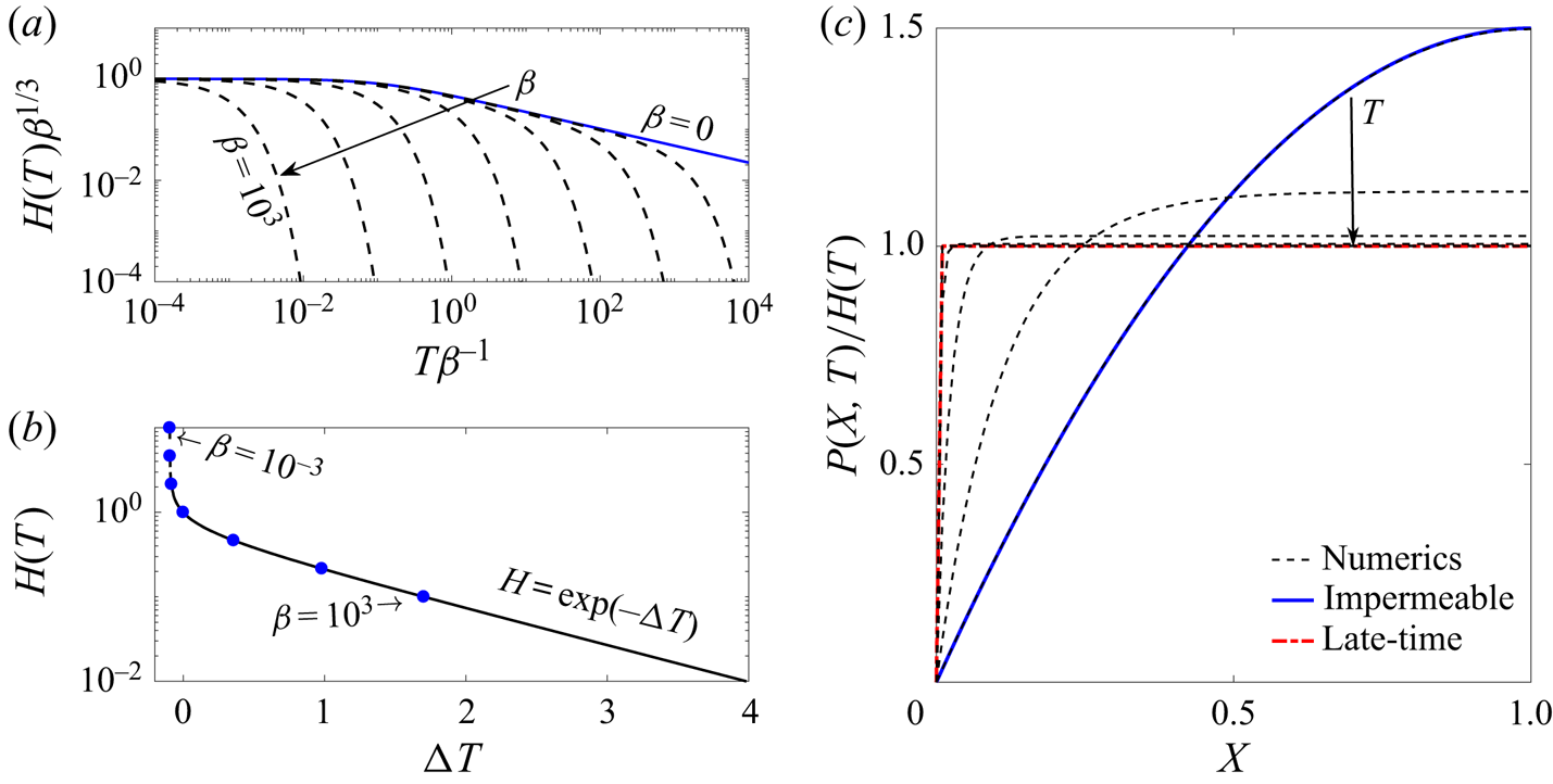
Figure 3. Aperture of a single fracture ( $n=1$) as a function of time for different values of $\beta ={H^*}^{-3}$. (a) Numerical solutions (dashed lines) using the rescaled aperture and time variables. Solutions are presented for seven different values in the range $\beta =[10^{-3},10^3]$ (i.e. ${H^*}=[0.1,10]$). The solid line is the analytic solution of the impermeable case ( $\beta =0$). (b) Time translated numerical solutions. The round markers signify the initial point of each translated solution. The curves were translated so that $H(T) = 1$ at $T=0$ for the ones that did achieve that value, and the others were placed to overlap. At late time the constant slope is the time exponent in the semi-logarithmic plot. (c) Numerical solution of the pressure field at different times (dashed lines), for $H^*=10$. The solutions are scaled by the instantaneous value of the aperture. The solid line (blue) is again the analytic solution of the impermeable case and the thick (red) dot-dashed line is the asymptotic solution for the pressure at late times (3.9).
3.4. Asymptotic investigation
We non-dimensionalized equation (2.9a) such that the two terms on the right-hand side, representing channel-parallel backflow and cross-channel leakage through the permeable wall, respectively, are in balance when  $H(T)= O(1)$.
When  $H(T) \gg 1$, the permeability is relatively small, flow through the permeable wall is negligible, and the channel-parallel flow dominates. Expanding the $\tanh$ function to the fifth order for large $H$ and substituting it back into the ODE (3.2a), we obtain, at leading order with an $O({H}^{-3})$ relative error,
 \begin{equation} \frac{\textrm{d} H}{\textrm{d} T}=-\frac{3}{H^2} \quad \Rightarrow \quad H(T)=\frac{1}{\left({H^*}^{-3}+9T\right)^{1/3}}. \end{equation}
This result is the solution for the impermeable case found by Dana et al. (Reference Dana, Zheng, Peng, Stone, Huppert and Ramon2018) after integration subject to the initial condition (2.10a). The solution (3.6) holds while  $H\gg 1$, i.e. for initial times $0\leqslant T\ll 1$ in the case $H^*\gg 1$. When ${H^*}^{-3}\ll T\ll 1$ it can be further simplified to the power law $H(T)\sim {(9T)^{-1/3}}$.
When  $H(T)\ll 1$, i.e. late times, or small initial aperture values, the cross-flow dominates the drainage and the channel-parallel flow becomes negligible. The ODE (3.2a) simplifies to
 \begin{equation} \frac{\textrm{d} H}{\textrm{d} T}=-H, \quad \Rightarrow \quad H(T)= C\exp{(-T)}, \end{equation}
where  $C$ is an arbitrary constant. If $H^*\ll 1$, then this solution is valid for all $T$ and the initial condition (2.10a) yields $C=H^*$. However, if $H^*\gtrsim 1$, then (3.7) is valid for late times $T\gg 1$, and does not have to satisfy the initial condition. Instead, $C$ depends on the detailed behaviour during the transition when $H = O(1)$.
The solution of the case  $H = O(1)$ is the full solution of the problem, where we cannot further simplify the ODE. However, we can use the full implicit solution (3.2b) to express the coefficient $C$ in the late-time asymptotic result (3.7b) in terms of the initial condition $H^*$. Equating the solutions (3.2b) and (3.7b), and taking the limit $H\rightarrow 0$, we obtain
 \begin{equation} \ln(C)=\ln(H^*)-\int_0^{H^*}H^{1/2}\tanh(H^{-3/2})\,\mathrm{d}H. \end{equation}
Furthermore, in the limit  $H^*\gg 1$, we obtain $C\approx \exp (-0.527)\approx 0.5904$. (In the limit $H^*\ll 1$, we recover $C=H^*$.) This shows, more generally, that if a solution is known to have the asymptotic behaviour $H \sim 9^{-1/3} (T + A)^{-1/3}$ for $H \gg 1$, where $A$ is some constant, then after the transition during which $H = O(1)$ and $T+A = O(1)$, the asymptotic behaviour is $H \sim C\exp (-T-A)$ for $H \ll 1$, with $C$ given above.
3.4.1. Pressure distribution
The time evolution of the pressure profile is plotted in figure 3(c), scaled by the instantaneous aperture value. When  $H(T)$ is large, both the pressure distribution and aperture behave as in the impermeable case (the blue solid line). Dana et al. (Reference Dana, Zheng, Peng, Stone, Huppert and Ramon2018, Reference Dana, Peng, Stone, Huppert and Ramon2019) provided complete solutions for such systems. When $H(T)$ is small, permeation is the main drainage mechanism. Neglecting the channel-flow term on the right-hand side of the hydrodynamic equation (2.9a) and combining with (3.7a), we obtain $P(X,T)\sim H(T)$ as evident by the scaled value approaching unity at late times. However, to satisfy the outlet boundary condition (2.10b), a boundary layer must form near the outlet. We can obtain the boundary layer solution by expanding the full profile (3.1a) to find
 \begin{equation} P(X,T)=\frac{\textrm{d} H}{\textrm{d} T}\left[\exp\left(-\frac{X}{H^{3/2}}\right)-1\right], \end{equation}
where  $H(T)$ is given by (3.7b). The size of the boundary layer thus obeys $H^{3/2}\ll 1$. This result is shown with a thick (red) dot-dashed line in figure 3(c) and is in good agreement with the late-time numerical results.
4. Solution for a fracture network
Advancing to the general case for a network of  $n$ generations, we discretized and reduced the equations to ODEs (see appendix A) as previously performed for the impermeable case by Dana et al. (Reference Dana, Peng, Stone, Huppert and Ramon2019). Numerical calculations were performed using the Matlab subroutine ODE23s.
In this section, we will show that the asymptotic dependence of the solution for a channel in a fracture network on the parameter  $H^*$ is similar to that displayed in previous sections for a single channel. Since a thorough analysis of the network behaviour in the impermeable case was conducted by Dana et al. (Reference Dana, Zheng, Peng, Stone, Huppert and Ramon2018, Reference Dana, Peng, Stone, Huppert and Ramon2019), in this section we only remark on the effects of substantial permeation on the general behaviour.
Two numerical solutions were obtained for the case of a bifurcated network with  $n=4$, for large and small values of $H^*$. Figures 4(ai) and 4(aii), showing the pressure distributions (dashed curves) for a large initial condition, exhibit an initial profile in which the bulk of the gradient is concentrated in the outlet channel, as found for the impermeable case. However, at late times, i.e. figure 4(aiii), the pressure profile tends to the profile of the apertures (solid curves). For small values of the initial condition, figure 4(b), the pressure profile immediately behaves like the aperture profile without going through the behaviour attributed to the impermeable regime. The shape of the pressure profile indicates that the driving force for the parallel flow is diminishing due to the increased leakage through the channel wall.

Figure 4. Non-dimensional numerical solutions of pressure  $P(X,T)/P_{max}$ (dashed lines) and aperture $H(X)/P_{max}$ (solid lines) for a network ( $n=4$) with two different magnitudes of initial condition: (a) $H^* = 100$; (b) $H^* = 0.1$. The results are scaled using the instantaneous maximum pressure $P_{max}$.
Figure 5(a) shows the time evolution of the channel apertures for the two cases from figure 4, and confirms that the impermeable  $T^{-1/3}$ behaviour is obtained when the apertures are large, i.e. $H(T) \gg 1$, while the permeation-dominated exponential decay is obtained when the apertures are small, i.e. $H(T) \ll 1$. For the case with initial aperture $H^* = 100$, the transition from $T^{-1/3}$ to $\exp (-T)$ coincides with the change in pressure profile from having a significant gradient driving the fluid along the outlet channel (figure 4aii) to being nearly spatially uniform within each channel (figure 4aiii). This transition means that each of the generations in the network now drains individually, independently of its neighbours (as parallel flow becomes negligible). However, since all channels drain exponentially with the same rate in the permeation-dominated regime, the aperture profile remains ‘frozen’ and is similar to that displayed in the impermeable regime, cf. figure 5(b,c). Conversely, when the initial aperture is small, a dominant cross-flow drainage immediately begins and the initial (uniform) aperture profile becomes ‘frozen in’ (figure 4b), rather than the aperture profile from the impermeable regime.
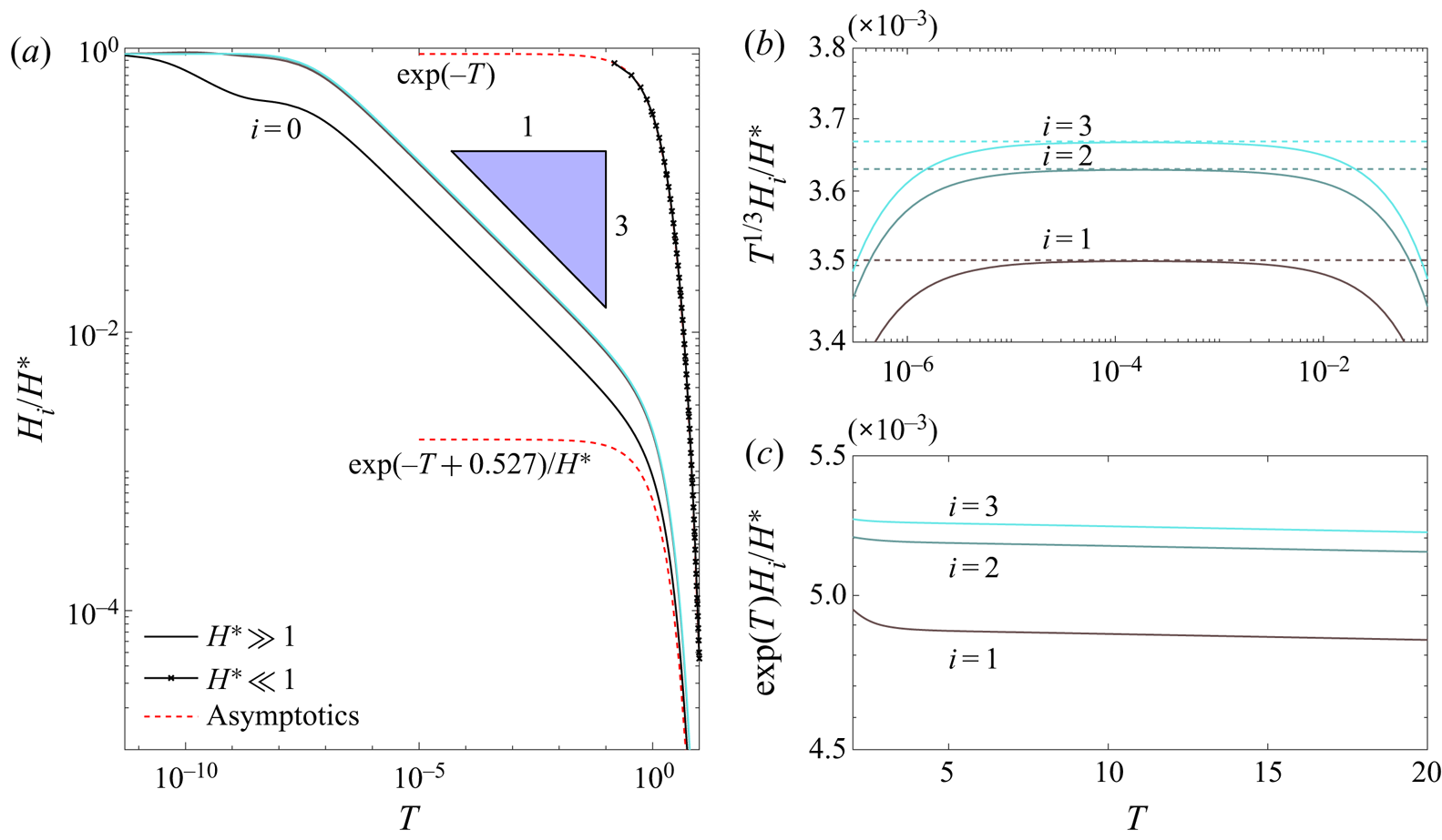
Figure 5. Non-dimensional numerical solutions for a network of four generations ( $n=4$) for two different magnitudes of $H^*={0.1,100}$ compared with asymptotic solutions. (a) Numerical solution for both small (in x-marked lines) and large (in solid lines) values of $H^*$ in time. The curves correspond with the curves in (b,c), under the appropriate rescaling. (b) Late-time numerical results for large $H^*$ scaled by the $-1/3$ power law. (c) Very-late-time numerical results for large $H^*$ scaled by the exponential of time.
5. Discussion
5.1. Comparison with constant-force models
To date, many studies have tackled the problem of squeeze flow with a constant force, the solution for which produces an asymptotic late-time dependence of a  $t^{-1/2}$ power law for channels with zero-curvature surfaces, e.g. Stone (Reference Stone2005). Others, e.g. Knox et al. (Reference Knox, Wilson, Duffy and McKee2015) and Venerus (Reference Venerus2018), have considered the addition of a porous boundary. Figure 6 shows the difference between our model and one considering a constant force on the boundary rather then the relaxation of a linear elastic one. For a constant force, the problem formulation remains exactly as defined in § 2.1, but the right-hand side in (2.9b) is set to a constant value equal to the force initially obtained in our elastic model, i.e. $\hat {E} h^*L$. One of the most interesting results it produces is that, for zero-curvature (i.e. flatter than parabolic) boundaries, contact between the two surfaces (i.e. $H(T)=0$) can be reached in inite time, because the aperture in the late-time permeable regime decreases linearly with time and the boundary velocity is constant (Ramon et al. Reference Ramon, Huppert, Lister and Stone2013; Knox et al. Reference Knox, Wilson, Duffy and McKee2015). This finite closing time is denoted by the dashed vertical line in figure 6. However, our elastic model produces a $t^{-1/3}$ power law for the impermeable regime and an exponential behaviour for the permeable one, in which a constant velocity cannot be reached. The differences between the two models arise from (2.9b), where the pressure on the boundary scales like $H$ (and thus decreases to zero with $H$), instead of some constant as in the case of a constant force. Although the exponential behaviour does not provide the same finite contact-time effect, this rapid decay accelerates the process and we can consider the idea of contact time using some finite aperture scale that can be attributed, for example, to surface roughness.
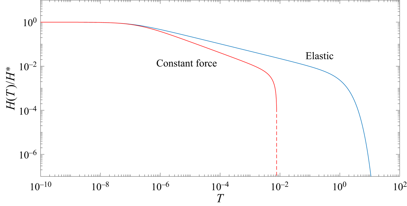
Figure 6. Comparison for a single channel between our model (with  $H^* = 100$) and a similar model with a constant force of non-dimensional value $H^* = 100$, so that at $T=0$ the applied force in both models is the same. The dashed vertical line denotes the contact time, i.e. $H(T)=0$, in the constant-force model.
5.2. Contact time
If we consider the walls of the channel to reach contact when the aperture has shrunk to a fraction  $\varepsilon \ll 1$ of its initial value, then we can define the contact time $T_{\varepsilon }$ by $H(T_{\varepsilon }) = \varepsilon H^*$. For example, figure 7 shows results for $\varepsilon =0.0001$, using the alternative scaling (3.3) based on the impermeable system. We observe that increasing the non-dimensional permeability $\beta$ drastically reduces the (rescaled) contact time $\tilde {T}_\varepsilon = T_\varepsilon \beta ^{-1}$, as is to be expected due to the exponential decay in the permeation-dominated regime.

Figure 7. Effect of permeability on volume and contact time for a single channel. (a) Retrieved volume relative to its initial value for a single channel for different values of the non-dimensional permeability  $\beta$. The values correspond to the times presented in (b) for the same value of $\beta$. (b) Rescaled contact time, $\tilde T_\varepsilon$ as a function of $\beta$, calculated for $\varepsilon =0.0001$. The dashed lines are asymptotic approximations corresponding with each regime (purely impermeable, transition and permeation dominated).
We can estimate the contact time asymptotically by substituting our assumed contact scale  $H(T_{\varepsilon })=\varepsilon H^*$ into the solutions obtained in § 3.4 and solving for $T_\varepsilon = \tilde {T}_\varepsilon \beta$. As can be seen in figure 7, there are three asymptotic regimes corresponding to different physics. For very small non-dimensional permeability $\beta \ll \varepsilon ^{3}$, the system remains in the impermeable regime until contact occurs, and so the contact time is given by $\tilde {T}_\varepsilon \sim 1/9\varepsilon ^3$ from (3.6b), which is naturally independent of $\beta$. For large $\beta \gg 1$, the system is always in the permeation-dominated regime, so the contact time is given by $\tilde {T}_\varepsilon \sim \ln (1/\varepsilon )/\beta$ from (3.7b). For the intermediate values, $\varepsilon ^3 \ll \beta \ll 1$, the system undergoes the transition (3.8) between regimes, which yields $\tilde {T}_\varepsilon \sim \ln (0.5904\beta ^{1/3}/\varepsilon )/\beta$.
5.3. Optimal outflow direction
Here, we give an example of how our model can be used to derive physical principles that can guide the analysis of more complicated systems. We consider a non-branching network with a rigidity gradient, i.e. a sequence of channels with increasing rigidity from ‘left’ (index  $i=0$) to ‘right’ (index $i=n-1$), and ask whether it is better to drain the network from the softer left end or from the more rigid right end, if the goal is to retrieve as much fluid volume from the outlet as possible.
We first focus on a case with  $n=4$ generations where the rigidity of each successive channel increases by a factor $\eta = 1.5$, and following Dana et al. (Reference Dana, Peng, Stone, Huppert and Ramon2019), we take the initial aperture profile to correspond to a spatially uniform static pressure of non-dimensional value $H^* = 10$. This results in the non-dimensional equations (2.9b) and (2.10a) being replaced by
 \begin{equation} \int_{0}^{1} P_i\,\mathrm{d}X= \eta^i H_i \quad \text{and} \quad H_i(0) = H^* \eta^{-i}. \end{equation}
Also, due to the lack of branching in the network, the factor  $2$ in (2.10d) is removed (cf. Dana et al. Reference Dana, Peng, Stone, Huppert and Ramon2019). For draining from the left end, the remaining equations are unchanged, but for draining from the right end, the locations of the zero-pressure and zero-flux boundary conditions (2.10b) and (2.10e) are interchanged.
Figure 8(a) shows the time evolution of the aperture of each channel, draining either from the softer left end (solid curves) or from the more rigid right end (dashed curves). We find that the drainage towards the softer, left end is much more rapid because any fluid that leaves through the outlet needs to pass the outlet channel, and a softer outlet channel has a larger aperture and hence a significantly decreased flow resistance. When draining towards the right end, the more rigid outlet channel closes rapidly and traps the fluid in the more open channels upstream, resulting in a slower drainage of the fluid. (The early-time temporary increase in upstream channel thickness occurs in response to the abruptly imposed outlet boundary condition (2.10b) and the requirement to satisfy the initially applied force on the boundary according to (2.9b).)

Figure 8. Results for a non-branching network with  $n=4$ generations, initial outlet aperture $H^*=10$, and rigidity factor $\eta =1.5$, comparing drainage from either the left softer (solid lines) or right more rigid (dashed lines) ends. (a) Evolution of the aperture. (b) Evolution of the volumes of fluid remaining in the network, retrieved via the outlet, and lost via permeation through the channel walls.
The consequence of the slower drainage is readily seen in figure 8(b), which shows the evolution of the volumes of fluid retrieved through the outlet, lost through permeation into the foundation and remaining in the system. The permeated volume initially increases at the same rate for the two cases, as it only depends on the pressure distribution which is initially similar. However, there is an immediate difference in retrieved volume, due to the differing outlet apertures. As the softer outlet system rapidly drains through the outlet (solid curves), the pressure in the network decreases and less fluid is lost by permeation. For the opposite case (dashed curves), the more rigid outlet traps a large amount of fluid inside the network at high pressure, resulting in the volume lost by permeation increasing and overtaking the volume retrieved via the outlet.
We conclude that in a system with a spatially varying rigidity, placing the outlet at the softer end rather than the more rigid end increases the outflow and reduces the volume lost by permeation. Figure 9(a) confirms that this also holds true for a more moderate rigidity factor  $\eta = 1.1$, over a range of network sizes ( $2 \leqslant n \leqslant 8$) and values of the non-dimensional permeability $\beta$. We also expect this principle to be insensitive to the details of the model employed, so that the conclusion also applies to more realistic systems. This expectation is also applicable to other results, such as the one depicted by figure 9(b), discussed below.

Figure 9. Comparison of drainage from either the left (solid curves) or right (dashed curves) ends of non-branching networks of various size ( $n=2,4,6,8$), showing the relative fraction of initial fluid volume retrieved at varying non-dimensional permeability $\beta = {H^*}^{-3}$. (a) Rigidity factor $\eta = 1.1$ and uniform permeability, i.e. $\kappa = 1$. (b) Permeability factor $\kappa = 2$ and uniform rigidity, i.e. $\eta =1$.
In a similar fashion, one can also consider a network with a permeability gradient (and, for simplicity, no branches and no variation in rigidity). Figure 10(a) shows the time evolution of the aperture of each channel, draining either from the less permeable outlet (solid curves, i.e. draining from left end) or from the more permeable outlet (dashed curves, i.e. draining from right end). The permeability of the leaking wall increases by a factor  $\kappa = 5$ with each successive channel from left to right. In this case, we find two competing effects. Initially, the network with a less permeable outlet loses fluid to permeation faster, because the pressure is higher near the tip (i.e. its opposite end). However, when permeation becomes significant, the walls of the more permeable channel also close faster, so that when located at the outlet this channel traps the fluid upstream and reduces the retrieved volume. For almost all parameter values studied, we found that the second effect is dominant, so that more volume is retrieved when draining from the lower-permeability end. Exceptions were found when $n$,
$n$,  $\kappa$ and the overall permeability were all small, for which draining from the higher-permeability end was more efficient, but only by a negligibly small amount.

Figure 10. Results for a non-branching network with  $n=4$ generations and a uniform rigidity (i.e. $\eta =1$), initial outlet aperture $H^*=10$, and permeability factor $\kappa =5$, comparing drainage from the left, less permeable (solid lines), or right, more permeable (dashed lines), ends. (a) Evolution of the aperture. The thickness of the line signifies the distance from the outlet, the outlet being the thickest. (b) Evolution of the volumes of fluid remaining in the network, retrieved via the outlet, and lost via permeation through the channel walls.
Figure 9(b) shows the volume retrieved from networks with a more moderate permeability factor,  $\kappa = 2$. We observe that, where there is a significant difference, draining from the left, less permeable, end of the network yields a larger retrieved volume compared with draining from the right, more permeable, end. This indicates that out of the two mechanisms discussed in the previous paragraph, trapping is typically the dominant one. This is because the more permeable outlet tends to close at a faster rate, trapping the fluids contained in the upstream of the network. This effect is further enhanced for larger network sizes, in which more fluid volume is contained upstream, taking longer durations to reach the outlet (Dana et al. Reference Dana, Zheng, Peng, Stone, Huppert and Ramon2018).
6. Summary
The present study extends the model of a fracture network introduced by Dana et al. (Reference Dana, Zheng, Peng, Stone, Huppert and Ramon2018) to account for the effects of permeable boundaries on the dynamics of its elastic relaxation. The permeation was modelled as linearly proportional to the local pressure, assuming negligible formation pressure.
For a single fracture, a solution is found (figure 3b) to which every solution is related by time translation (3.2b). When the aperture is sufficiently large, the parallel flow is dominant and the solution tends to a  $T^{-1/3}$ time dependence as in the impermeable case solved asymptotically by Lai et al. (Reference Lai, Zheng, Dressaire, Ramon, Huppert and Stone2016) and Dana et al. (Reference Dana, Zheng, Peng, Stone, Huppert and Ramon2018, Reference Dana, Peng, Stone, Huppert and Ramon2019). However, when the aperture is sufficiently small, the cross-flow is dominant and the solution decays exponentially in time. In this exponential regime, the pressure profile tends to the aperture, i.e. $P(X,T)\sim H(T)$, with a boundary layer forming near the outlet of the channel to satisfy the zero-pressure boundary condition.
The model is then extended to consider drainage from a network of channels, considering spatially varying rigidity and permeability. Networks were shown to be dominated by the impermeable regime (Dana et al. Reference Dana, Zheng, Peng, Stone, Huppert and Ramon2018) when the apertures are large enough. However, when the cross-flow is dominant, the channels behave independently and the inter-channel flow becomes negligible. Thus, when the system has sufficient time to tend to the asymptotic impermeable regime, we find the exponential behaviour to exhibit a ‘frozen’ profile of the same aperture ratios. Conversely, when the initial condition is very small, and the channels immediately behave independently, the ‘frozen’ profile is given by the initial condition rather than by a universal late-time profile.
While the details of the numerical and asymptotic results obtained in this paper are specific to our model, the physical principles identified can be expected to apply also to more realistic and complex fracture networks with different (and even partially unknown) elasticity and permeability characteristics. Initially and for large apertures, the flow towards the outlet is dominant and the network behaves as if impermeable, but as the apertures shrink, permeability becomes significant, which accelerates the closure of the apertures. If the elasticity and permeability are such that pressure scales linearly with both aperture and leakage, then an exponential decay can be expected at late times when permeability is dominant. The permeation results in fluid being lost into the foundation rather than being retrieved via the outlet.
If the network has a gradient in rigidity, e.g. figure 8(b), then draining the network from the softer end results in a larger volume of fluid being retrieved. For a spatially varying wall permeability, e.g. figure 10(b), results mainly indicated that the retrieved volume is maximized when draining from the less permeable end when the overall contribution of permeation is large.
We have presented an investigation of the effects attributed to leakage from channel walls on the elastic relaxation process of model network structures. This work was motivated, in part, in an attempt to develop a framework that may inform design of fluid waste management from hydraulic fracture networks. These may even, in the future, assist in the analysis of flow data from wells to gain insight into the fractured formation, as well as decision making in the fracturing process. Additionally, the obtained concepts may be relevant to various systems that include squeezing of viscous fluids by a permeable surface, e.g. in the modelling of diarthrodial joints, soft robotics and various microfluidic applications. Further advances towards such implementations should include validation against experimental and field observations.
Funding
A.D. acknowledges the support from the Nancy and Stephen Grand Technion Energy Program (GTEP). This research has been supported by the Israeli Ministry of National Infrastructures, Energy and Water Resources under the student scholarship program for degrees in the field of energy.
Declaration of interests
The authors report no conflict of interest.
Appendix A
To numerically solve the system formulated in § 2.2, we evolve the system forward using an explicit method. That means that at each time step we know the present  $H_i$ and need to calculate $\mathrm {d} H_i/\mathrm {d} T$ by first solving an algebraic system of equations for the discrete pressure and flux variables, $\hat {p}_i=P_i(0)$ and $\hat {q}_i=\alpha ^iH_i^3 {\partial P_i}/{\partial X}|_{(0,T)}$.
Following the discretized method described by Dana et al. (Reference Dana, Peng, Stone, Huppert and Ramon2019), we obtain the set of linear algebraic equations
 \begin{align} &\alpha^i H_i^3\frac{\tilde \beta_i}{2}\left[\coth\left(\frac{\tilde \beta_i}{2}\right)+\frac{1}{\coth\left(\dfrac{\tilde \beta_i}{2}\right)-\dfrac{2}{\tilde \beta_i}}\right]\hat p_i + \hat q_i\\ &\quad +\alpha^i H_i^3\frac{\tilde \beta_i}{2}\left[-\coth\left(\frac{\tilde \beta_i}{2}\right)+ \frac{1}{\coth\left(\dfrac{\tilde \beta_i}{2}\right)-\dfrac{2}{\tilde \beta_i}}\right]\hat p_{i+1} =\frac{\alpha^i\eta^i\tilde\beta_i H_i^4}{ \coth\left(\dfrac{\tilde\beta_i}{2}\right)-\dfrac{2}{\tilde \beta_i}}\nonumber \end{align}
 \begin{align} &\quad\left[{\frac{1}{\sinh\left({\tilde\beta_i}\right)}-\frac{1}{\tilde \beta_i} }\right]\hat q_i +{\alpha^i\tilde\beta_i H_i^3}\hat p_{i+1}-\left[ \coth\left({\tilde\beta_i}\right)-\frac{1}{\tilde \beta_i}\right]\hat q_{i+1}={\alpha^i\eta^i\tilde\beta_i H_i^4}, \end{align}
where  $\tilde \beta _i={H_i^{-3/2}}$. Equations (A1) contain four discrete variables, and combined with boundary conditions $\hat p_0=0,\,\hat q_n=0$, we obtain a tridiagonal matrix.
After solution using a traditional tridiagonal matrix algorithm in each time step, the temporal evolution is given by
 \begin{equation} \frac{\textrm{d} H_i(T)}{\textrm{d} T}=\frac{\tilde \beta_i}{2} { \alpha ^{-i} \left(\hat q_{i+1}-\hat q_i\right) \coth \left(\frac{\tilde \beta_i}{2}\right)}-\frac{1}{2} \left(\hat p_i+\hat p_{i+1}\right). \end{equation}


 Open access