


1. Introduction
Active matter describes systems in which the elements extract energy from their surroundings and convert it into mechanical work, leading to systems which are not in thermodynamic equilibrium. Active matter displays phenomena ubiquitous in a wide range of physical and biological systems, including but not limited to animal herds and suspensions of bacteria (Marchetti et al. Reference Marchetti, Joanny, Ramaswamy, Liverpool, Prost, Rao and Simha2013; Prost, Jülicher & Joanny Reference Prost, Jülicher and Joanny2015; Needleman & Dogic Reference Needleman and Dogic2017; Doostmohammadi et al. Reference Doostmohammadi, Ignés-Mullol, Yeomans and Sagués2018).
Due to the continuous energy injection of the active constituent particles, the active fluid's chaotic nature emerges, known as active turbulence (Wensink et al. Reference Wensink, Dunkel, Heidenreich, Drescher, Goldstein, Löwen and Yeomans2012; Bratanov, Jenko & Frey Reference Bratanov, Jenko and Frey2015; Doostmohammadi et al. Reference Doostmohammadi, Shendruk, Thijssen and Yeomans2017; Urzay, Doostmohammadi & Yeomans Reference Urzay, Doostmohammadi and Yeomans2017; Alert, Casademunt & Joanny Reference Alert, Casademunt and Joanny2022). In such a chaotic flow, the kinetic energy of micro-scale elements is transferred to a passive body immersed in the active fluid such that the body experiences a mechanical force on its boundaries. If the exerted energy is sufficiently high, the body could undergoes deformation (Paoluzzi et al. Reference Paoluzzi, Di Leonardo, Marchetti and Angelani2016), translation (Wu et al. Reference Wu, Lv, Zhao and Ai2018), rotation (Angelani, Di Leonardo & Ruocco Reference Angelani, Di Leonardo and Ruocco2009) or their combination.
Considering the induced motion of passive immersed bodies, the question may arise as to whether the active flow can also generate vibrational motion due to its chaotic and turbulent nature. As such, it should be possible to induce a constructive oscillatory motion on a flexible body, possibly made of a piezoelectric material that can be used as a sensor to extract the physical properties of the active fluid.
Generally, the behaviour of active nematics is affected mainly by fluid activity and elastic constant. Our recent study also showed that viscosity has a significant role by introducing the inertia effect to the active nematics system (Saghatchi, Yildiz & Doostmohammadi Reference Saghatchi, Yildiz and Doostmohammadi2022b). The measurement of these parameters is experimentally challenging (Frishman & Keren Reference Frishman and Keren2021), and the secondary properties are often used to extract these main parameters. Currently, the most common method to assess the activity is to measure the adenosine triphosphate (ATP), the motor cluster, microtubules or polyethylene-glycol concentrations (Henkin et al. Reference Henkin, DeCamp, Chen, Sanchez and Dogic2014; Doostmohammadi et al. Reference Doostmohammadi, Ignés-Mullol, Yeomans and Sagués2018), among others. Researchers have been working on numerical procedures such as machine learning algorithms (Colen et al. Reference Colen2021) to find an alternative approach to measure the physical properties directly.
Considering the aforementioned issues, we placed a cantilever beam in active nematics and numerically analysed the induced vibration. We used a continuum model for the active nematics and combined it with a fluid-structure interaction (FSI) solver to calculate the imposed force on the beam and, consequently, analyse its motion. We investigated the effects of vorticity and velocity field on the beam oscillation. Then, we demonstrated the impact of three critical parameters, that is, fluid activity, viscosity and its elastic constant, on the beam peak frequency and proposed a mathematical relationship that makes direct measurement feasible for future practical utilization.
2. Methods
2.1. Governing equations
In this study, a 2-D continuum approach is implemented for modelling the nematic phase where the nematic tensor  $\boldsymbol{\mathsf{Q}}$ is used to describe the nematic orientation $\boldsymbol {n}$ and its order $q$ as $\boldsymbol{\mathsf{Q}} = 2q (\boldsymbol {nn} - (\boldsymbol{\mathsf{I}}/2))$, where $\boldsymbol{\mathsf{I}}$ denotes the identity tensor. The Beris–Edwards equation is used to evolve $\boldsymbol{\mathsf{Q}}$ in time as (Beris & Edwards Reference Beris and Edwards1994)
 \begin{equation} \frac{\partial \boldsymbol{\mathsf{Q}}}{\partial t}+(\boldsymbol{u}\boldsymbol{\cdot}\boldsymbol{\nabla})\boldsymbol{\mathsf{Q}} - \boldsymbol{\mathsf{S}} = \varGamma \boldsymbol{\mathsf{H}}, \end{equation}
where
 $$\begin{gather} \boldsymbol{\mathsf{S}} = \lambda \boldsymbol{\mathsf{E}}-({\boldsymbol{\mathsf{\Omega}}} \boldsymbol{\cdot}\boldsymbol{\mathsf{Q}}-\boldsymbol{\mathsf{Q}}\boldsymbol{\cdot}{\boldsymbol{\mathsf{\Omega}}}); {\boldsymbol{\mathsf{\Omega}}} =\frac{1}{2}[{(\boldsymbol{\nabla} \boldsymbol{u})^{\dagger}- \boldsymbol{\nabla} \boldsymbol{u}}], \quad \boldsymbol{\mathsf{E}}=\frac{1}{2} [{\boldsymbol{\nabla} \boldsymbol{u} + (\boldsymbol{\nabla} \boldsymbol{u})^{\dagger}}], \end{gather}$$
 $$\begin{gather}\boldsymbol{\mathsf{H}} ={-}\frac{\delta \mathcal{F}}{\delta \boldsymbol{\mathsf{Q}}} + \frac{\boldsymbol{\mathsf{I}}}{2} {\rm Tr} \left(\frac{\delta \mathcal{F}}{\delta \boldsymbol{\mathsf{Q}}}\right), \quad \mathcal{F} = \frac{1}{2}K(\boldsymbol{\nabla} \boldsymbol{\mathsf{Q}})^{2} +\frac{A}{2}\left(q^2-\frac{1}{2} \text{Tr}[\boldsymbol{\mathsf{Q}}^2]\right)^{2}. \end{gather}$$
In these equations,  $t$,
$t$,  $\boldsymbol {u}$, ${\boldsymbol{\mathsf{\Omega}}}$ and $\boldsymbol{\mathsf{E}}$, respectively, represent time, velocity, vorticity tensor and rate of strain tensor. Here $\boldsymbol{\mathsf{S}}$ is the generalized nonlinear advection term which is controlled by tumbling parameter ( $\lambda$), and $\boldsymbol{\mathsf{H}}$ stands for the molecular field, which relates the relaxation of $\boldsymbol{\mathsf{Q}}$ to the minimum of the free energy ( $\mathcal {F}$) and it is controlled by the rotational diffusivity ( $\varGamma$). Free energy, $\mathcal {F}$, includes two parts, elastic and bulk free energies, which are regulated by elastic constant ( $K$) and the coefficient $A$, respectively (Saghatchi, Kolukisa & Yildiz Reference Saghatchi, Kolukisa and Yildiz2022a).
The velocity field is computed by the coupled solution of the conservation of mass and linear momentum equations:
 $$\begin{gather} \boldsymbol{\nabla} \boldsymbol{\cdot} \boldsymbol{u} = 0, \end{gather}$$
 $$\begin{gather}\rho \left(\frac{\partial \boldsymbol{u}}{\partial t}+(\boldsymbol{u}\boldsymbol{\cdot}\boldsymbol{\nabla})\boldsymbol{u}\right) = \boldsymbol{\nabla} \boldsymbol{\cdot}{{\boldsymbol{\mathsf{\Pi}}}}, \end{gather}$$
where  $\rho$ represents the density, and ${\boldsymbol{\mathsf{\Pi}}} =-p\boldsymbol{\mathsf{I}}+{\boldsymbol{\mathsf{\Pi}}}_{viscous}+ {\boldsymbol{\mathsf{\Pi}}}_{active}$ is the stress tensor which includes the pressure ( $p$), viscous term ( ${\boldsymbol{\mathsf{\Pi}}}_{viscous}=2\mu \boldsymbol{\mathsf{E}}$) and active term ( ${\boldsymbol{\mathsf{\Pi}}}_{active}=-\zeta \boldsymbol{\mathsf{Q}}$). Parameters $\mu$ and $\zeta$ denote the dynamic viscosity and the activity coefficient, respectively.
The solid part of the model is governed by the following equation:
 \begin{equation} \rho \left(\frac{\partial \boldsymbol{v}}{\partial t}+(\boldsymbol{v}\boldsymbol{\cdot}\boldsymbol{\nabla})\boldsymbol{v}\right) = \boldsymbol{\nabla} \boldsymbol{\cdot}{{\boldsymbol{\mathsf{\sigma}}}_{\boldsymbol{s}}}, \end{equation}
where  ${\boldsymbol{\mathsf{\sigma}}} _s$ denotes the Cauchy stress tensor and $\boldsymbol {v}$ represents the displacement vector. Assuming linear geometry and elastic material, Hookean tensor is defined as ${\boldsymbol{\mathsf{\sigma}}} _s=2G \boldsymbol {{\boldsymbol{\mathsf{\epsilon}}} }+(\kappa - \frac {2}{3}G) {\rm Tr}[{\boldsymbol{\mathsf{\epsilon}}} ]\boldsymbol{\mathsf{I}}$, where $G$ and $\kappa$ stand for the shear and bulk modulus, respectively, and ${\boldsymbol{\mathsf{\epsilon}}} =\frac {1}{2}\left [ \boldsymbol {\nabla } \boldsymbol {v} + (\boldsymbol {\nabla } \boldsymbol {v})^{\dagger} \right ]$ is the displacement gradient tensor.
2.2. Numerical scheme
To solve (2.1) through (2.4) numerically, the OpenFOAM package (Weller et al. Reference Weller, Tabor, Jasak and Fureby1998) is used along with the solids4foam toolbox (Cardiff et al. Reference Cardiff, Karač, Jaeger, Jasak, Nagy, Ivanković and Tuković2018) which is responsible for the coupling of the fluid part with the solid part and performs the FSI analysis where both packages employ the finite volume method (FVM).
Utilizing the partitioned approach, the whole computational domain is decomposed into two regions (fluid and solid) using the Dirichlet–Neumann procedure. As such, fluid and solid models are solved separately. The velocity at the fluid–solid interface is used as a boundary condition in the solution of the fluid domain, while the solid part uses the exerted force by the fluid on the interface. Consequently, these two solutions are coupled by dynamic (continuity of force) and kinematic (continuity of displacement and velocity) conditions on the fluid–solid interface by the Dirichlet–Neumann coupling scheme and utilize the Aitken adaptive under-relaxation procedure (Tuković et al. Reference Tuković, Karač, Cardiff, Jasak and Ivanković2018). The discretization schemes for each separate term in the governing equations are summarized in table 1. Pressure and velocity coupling throughout the fluid domain is carried out by the pressure-implicit with splitting of operators (PISO) algorithm (Versteeg & Malalasekera Reference Versteeg and Malalasekera2007).
Table 1. The discretization schemes that are used in this study (Moukalled, Mangani & Darwish Reference Moukalled, Mangani and Darwish2016).

The solution domain consists of a square region with a cantilever beam located at the middle point of the bottom boundary (see figure 1). A no-slip boundary condition is applied on all boundaries including the fluid–solid interface, while the zero-gradient condition is used for  $\boldsymbol{\mathsf{Q}}$. The structured Cartesian grid with $256\times 256$ is used to discretize the domain and the Courant–Friedrichs–Lewy (CFL) condition is enforced to control the solution time-step size. Initially, zero velocity field is applied with uniform nematic orientation $\boldsymbol {n}$ in the horizontal direction with a slight perturbation, and the results are evaluated at the time step at which steady state is statistically attained.

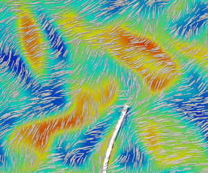
Figure 1. Schematic representation of the problem which includes a cantilever beam inside active nematics. Nematic particles and the orientation vector are represented in the inset.
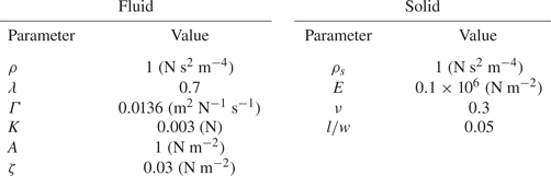
The main parameters used in this study are tabulated in table 2. In this table,  $E$ and $\nu$, respectively, represent the elastic modulus and Poisson's ratio, and $l/w$ is the length-to-thickness ratio of the beam. Based on the values in table 2, we define natural frequency of transverse vibration of a cantilever beam as $\omega ^*=(\beta l)^2\sqrt {{EI}/(\rho _s Al^4)}$, where $\beta l=1.875104$, $I$ is the area moment of inertia, $A$ represents the cross-sectional area, and $l$ is the beam length (Rao Reference Rao2011). Consequently, dimensionless time and frequency become $t\omega ^*$ and $\omega /\omega ^*$, respectively, where $\omega =1/t$. Since the activity and viscosity are the important parameters in our study, we define dimensionless activity and viscosity as $\zeta /A$ and $\mu \varGamma$, respectively.
Table 2. Values used in the numerical simulations, unless stated otherwise.
3. Results
We begin with the qualitative representation of the beam motion and flow field in the physical domain. We take  $\zeta =0.01$ and $K=0.05$, and the simulations are performed for the beams with two different values of elastic modulus, i.e. $E=0.01$ KPa and $E=1.0$ KPa (figure 2). Beam with lower elastic modulus imitates soft material such as biological tissue, which can easily bend under the effect of active stress. The beam bending is related to the flow dynamics, as shown in figure 3(a). In this sub-figure, velocity vectors are shown in vicinity of the beam. Clearly, magnitude of beam deformation and its orientation are controlled by the dominant direction of velocity vectors. If two vortices appear on different sides of the beam, the strongest one determines the bending direction as shown in figure 3(a). To further elaborate, when the strongest vortex (or vortices) travels inside the domain and moves towards the beam, it exerts forces on the beam and deforms it in the same direction. From an energy perspective, fluid elements inside these vortices posses a high amount of kinetic energy. If these kinetic energies that are transferred to the beam elements are high enough to surpass the beam's elastic potential energy and inertial force, the beam deforms and deflects. Thus, as the exerted force is more concentrated towards the beam tip, beam deflection is expected to be higher. Vortices are being moved in the domain due to the interactions of defects and the change in the director field (figure 3b). As a consequence of these periodic processes, a random excitation is imposed on the beam, leading to random vibration. Specifically, the maximum or peak oscillation frequency of the beam is associated with the frequency of instabilities due to the formation and annihilation of topological defects in active nematics.
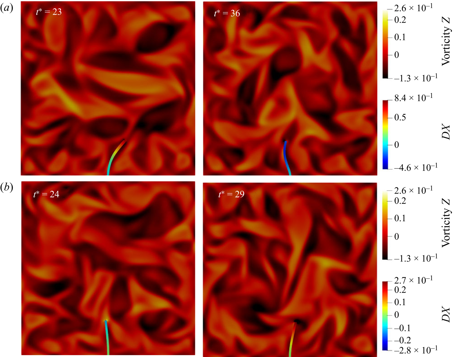
Figure 2. Vorticity and the beam horizontal displacement ( $DX$) contours at different times ( $t^* \approx t\omega ^* \times 10^{-2}$) for a beam with high elastic modulus (a), and low elastic modulus (b), correspond with $E=0.01$ KPa and $E=1.0$ KPa, respectively.

Figure 3. Flow and nematics characteristics in the domain close to the beam at  $t\omega ^* \approx 37 \times 10^{-2}$ (left column) and $t\omega ^* \approx 81 \times 10^{-2}$ (right column). (a) Vorticity, beam displacement and the velocity vectors. (b) Nematics director and their order of magnitude. (c) Effect of beam presence on the kinetic-energy spectrum. The beam consumes the kinetic energy of very high- and very low-scale vortices for its bending and oscillatory motion. Inset (I) represents the same plot in semi-log scale, and (II) is the kinetic-energy differences between flow with and without beam.
The kinetic-energy spectra can best represent quantitative features of the energy transfer to the beam, which characterizes the associated kinetic energy  $E_k=\tfrac {1}{2}\langle \hat {u}_i(k) \hat {u}_i(k) \rangle$ at different scales. Figure 3(c) illustrates the kinetic-energy spectrum for the wavenumber $k$, considering either the presence or the absence of the beam. Characteristic length scale $l_a=\sqrt {K/\zeta }$ is used to normalize the wavenumber. As inferred from this figure, energy at higher and lower ranges of wavenumbers is considerably lower for the test cases where the beam is placed in the computational domain than the test case without beam. This observation indicates that the fluid energy is transferred on the beam mainly at relatively low and high wavenumbers, respectively corresponding to the large-scale and small-scale vortices, and thereby leads to the oscillatory motion of the beam. It should be noted that no significant difference in kinetic energy at high wavenumbers is observed for the beams with small and high elastic modulus. However, at relatively low wavenumbers, the kinetic energy for the beam with high elastic modulus lies below that with low elastic modulus, showing that the former beam consumes a higher amount of large-scale vortices energy for its oscillation. Additionally, the semi-log plot of the energy spectra given as the inset I of figure 3(c) indicates an exponential decay rather than the algebraic one as a function of the wavenumber for the cases with and without the beam. Furthermore, we calculate the kinetic-energy difference between the cases with the beam and the case without the beam, which are presented in the inset II of figure 3(c). This figure shows a maximum point at $kl_a \approx 0.5$, denoting that the beam consumes the majority of the fluid energy for its oscillation from the large-scale vortices.
As mentioned above, fluid physical properties such as activity and viscosity could affect the beam vibration. As reported by Giomi (Reference Giomi2015), the typical time scale for the creation and annihilation of topological defects  $t_a$ is predominantly dictated by the active circulation $t_a \sim 1/\omega _v$. Moreover, topological defects move primarily along the edge of the vortices at approximately constant angular velocity $\omega _v \approx \zeta /\mu$. Consequently, the time scale for the creation and annihilation of topological defects is proportional to the ratio of $\zeta /\mu$. Recalling that maximum or peak oscillation frequency of the beam has been associated with the frequency of defect creation and annihilation, we conjecture that the beam tends to be stimulated accordingly, leading to the beam's oscillatory motion with the frequency proportional to $\zeta /\mu$. We first investigate the beam vibration under the different values of activity parameters, $\zeta$, to verify this claim. The value of $E=0.1\ {\rm MPa}$ is taken for the beam elastic modulus to represent an actual piezoelectric transducer (Elvin, Elvin & Senderos Reference Elvin, Elvin and Senderos2018). Beam tip displacement is monitored during the simulation and plotted as a function of dimensionless time, as shown in figure 4(a). This figure also presents the impact of activity on the vibrational motion of the beam. It is observed that a rise in the activity parameter increases the displacement amplitude. Physically, enhancing the activity is equivalent to injecting a higher amount of energy into the fluid elements. Consequently, when transferred to the beam, this energy could deflect the beam more and lead to a higher amount of displacement.

Figure 4. Results for a cantilever beam within the fluid with different activities: (a) time history of the beam's normalized deflection (the inset magnifies the small span of the vibration history); (b) Fourier spectrum; (c) frequency vs activity (linear relation is seen and demonstrated with a dashed line representing the regression analysis). Panel (d) represents the vorticity and beam deflection contours for  $\zeta /A=0.12$, $0.06$, $0.03$ and $0.015$ from top to bottom row.
To scrutinize the activity influence on the vibration frequency, we performed a fast Fourier transform (FFT) analysis to convert the displacement from a time domain to the frequency domain (Moin Reference Moin2010). Due to the non-deterministic nature of the excitation, multiple frequency peaks exist in the FFT curve. Since the maximum frequency peak is of interest, a moving average filter (MAF) is used to smooth out the FFT curve and remove the unnecessary noises (Smith Reference Smith1997), and the resultant curves are given in figure 4(b). As shown in this figure, the activity parameter alters the maximum or peak frequency such that the peak frequency shifts towards a higher value with the increase in activity. To obtain a possible correlation between the peak frequency and the activity parameter, we performed the simulation for various values of activity parameters and presented the results in figure 4(c). Interestingly, a linear correlation is observed for the peak-frequency versus activity parameter. The dashed line in figure 4(c) is the linear regression resulting from this correlation, showing an apparent linear relationship between peak frequency and activity. Qualitatively, recalling that a higher value of activity parameter is equivalent to a higher energy injection into the active nematic system. This increases the energy of vortices thereby intensifying their angular velocity  $\omega _v$, and also breaks large vortices into smaller ones (figure 4d). Essentially, the higher the activity or energy injection, the higher the angular velocity of vortices. Vortices with smaller sizes and higher velocities can move quickly and with higher frequency in the domain. These small yet strong vortices continuously collide with the beam and result in high beam-vibration frequency. Experimentally, the slope of the peak-frequency versus activity curve ( $\alpha$ in figure 4c) is obtainable through calibrating the piezoelectric transducer whereby it becomes possible to measure the fluid activity parameter.
It is also worthwhile to check the dependency of the peak frequency on the bulk viscosity  $\mu$ of the active fluid as well. Figure 5 demonstrates the variation of peak frequency as a function of dimensionless viscosity. As shown in this figure, the viscosity has an inverse and approximately reciprocal relationship with the peak frequency. A log–log diagram is also presented as an inset of this figure to illustrate this behaviour better, meaning that the peak frequency can be expressed by $\approx f(1/\mu )$ function. This behaviour can physically be explained considering the energy dissipation mechanism. Namely, the larger the viscosity, the higher the frictional force, which can dissipate the energy of small-scale vortices. Remembering the role of small-scale vortices in the beam oscillatory movement, an increase in the viscosity reduces peak frequency. Meanwhile, active nematics with lower viscosity fail to provide a substantial frictional mechanism to dissipate the energy of small-scale vortices, resulting in an increase in the imposed energy to the beam.

Figure 5. Effect of viscosity on the beam peak frequency. Inset shows the same data in the log–log scale, indicating the reciprocal relationship between viscosity and the peak frequency. The effect of viscosity on the size of vortices is also shown for two different viscosity values.
It is worth noting that the numerical investigation is also performed to examine the impact of the elastic constant  $K$ of active fluid on the beam frequency; however, no significant effect is observed. Recalling the characteristic length scale in active nematics, i.e. $l_a=\sqrt {K/\zeta }$, one may expect that the variation in elastic constant $K$ should change the length scale and vortices sizes. Referring to discussion provided to understand the correlation between the activity/viscosity and peak frequency, this variation should also lead to changes in the peak frequency. However, in the case of elastic constant, it should be noted that $K$ is also responsible for penalizing gradients in the nematic orientation, hence for the free energy ( $\mathcal {F}$). Consequently, the balance between $\mathcal {F}$ and vortex size determines the resultant frequency, which undergoes insignificant change with the variation in $K$, as our results show. In other words, the elastic constant does not participate in either injection or dissipation of the energy to/from the vortices, whereas both of them are responsible for determination of the system's time scale, hence the beam frequency.
4. Conclusions
In this study, we present a numerical method to solve the continuum model of active nematics which is combined with an FSI solver to simulate the vibration induced by active turbulence. For this purpose, we place a cantilever beam inside the active nematics and investigate the effect of important active fluid parameters such as activity, viscosity and elastic constant on the beam oscillatory motion. We provide qualitative data, including vorticity field and nematic ordering to investigate the beam dynamics.
Our results show that vortex formation that initiates from the symmetry breaking in the nematic ordering plays a dominant role in beam deflection. We also indicate that the size, strength and position of vortices determine the direction and magnitude of beam deflection. Using the kinetic-energy spectrum, we demonstrate that both large- and small-scale vortices play a primary role in the beam oscillatory motion by transferring the kinetic energy between active fluid and beam, with the contribution of former is higher.
We quantify the beam oscillation using FFT analysis on the beam tip displacement data and calculate the beam peak frequency. Our results show that the activity and beam peak frequency are linearly correlated. The physical phenomena behind this correlation is explained through considering the nematic activity (which influences the energy injection into the system) and its role on increasing the angular velocity and reducing the size of vortices. Our results further reveal the reciprocal relationship between viscosity and beam peak frequency, which stems from the fact that viscosity dissipates the energy of small-scale vortices. Finally, we analyse the impact of the elastic constant of active nematics on the beam peak frequency and show that its effect is insignificant.
The results presented in this study propose a potential novel method to measure the critical parameters of active nematics that play a significant role in determining its flow behaviour using the beam peak frequency concept. This method can be an alternative to the current challenging measurement techniques that determine the activity, for example, by measuring secondary parameters such as ATP, the motor cluster, microtubules or polyethylene-glycol concentration (Henkin et al. Reference Henkin, DeCamp, Chen, Sanchez and Dogic2014; Doostmohammadi et al. Reference Doostmohammadi, Ignés-Mullol, Yeomans and Sagués2018).
Declaration of interests
The authors report no conflict of interest.


 Open access