


1. Introduction
Turbulent scalar dispersion in a turbulent boundary layer (TBL) flow has applications in thermal, environmental, petroleum, mechanical and aerospace engineering. The scalar dispersion of a plume released from a point source has been widely studied in rough-wall TBL flows (e.g. Robins Reference Robins1978; Fackrell & Robins Reference Fackrell and Robins1982a,Reference Fackrell and Robinsb; Yee et al. Reference Yee, Kosteniuk, Chandler, Biltoft and Bowers1993; Nironi et al. Reference Nironi, Salizzoni, Marro, Mejean, Grosjean and Soulhac2015; Iacobello et al. Reference Iacobello, Marro, Ridolfi, Salizzoni and Scarsoglio2019) due to interest in the dispersion of hazardous materials or pollutants in the atmosphere. For canonical smooth-wall TBL flow, the velocity statistics and mechanisms of momentum transport have been well studied (e.g. Adrian, Meinhart & Tomkins Reference Adrian, Meinhart and Tomkins2000; Ganapathisubramani, Longmire & Marusic Reference Ganapathisubramani, Longmire and Marusic2003; Marusic et al. Reference Marusic, McKeon, Monkewitz, Nagib, Smits and Sreenivasan2010); however, fewer studies have focused on scalar dispersion in this scenario (e.g. Crimaldi & Koseff Reference Crimaldi and Koseff2001, Reference Crimaldi and Koseff2006; Crimaldi, Wiley & Koseff Reference Crimaldi, Wiley and Koseff2002) and only a handful focus on the relationship between the concentration and velocity fields (e.g. Talluru, Philip & Chauhan Reference Talluru, Philip and Chauhan2018; Young, Webster & Larsson Reference Young, Webster and Larsson2022). While smooth-wall configurations do not occur as frequently in nature as roughness, it is still important for phenomenological understanding as it is often used as a baseline to study the effects of other boundary conditions, such as roughness, free-stream turbulence, pressure gradients, etc. Moreover, scalar dispersion of a ground-level point source in a smooth-wall TBL specifically, has applications in heat and mass transport, which includes film cooling of turbine blades and heat and mass transfers in pipe flows.
Although there is strong experimental evidence of outer layer similarity of turbulence structures in smooth- and rough-wall TBLs (Raupach, Antonia & Rajagopalan Reference Raupach, Antonia and Rajagopalan1991), there are phenomenological differences in the viscous sublayer (VSL) for smooth-wall and roughness sublayer (RSL) for rough-wall TBLs. Schultz & Flack (Reference Schultz and Flack2007) demonstrated outer layer similarity for TBL flows at sufficiently high Reynolds number and small roughness to boundary-layer thickness height. Blackman et al. (Reference Blackman, Perret, Calmet and Rivet2017) investigated the rough-wall TBL from a turbulent kinetic energy budget perspective and showed energy dissipation via forward scatter (transfer of energy from large to small scales) and backscatter (small to large scales) events were linked to coherent vortices that are not dissimilar to smooth-wall TBL. In the RSL, however, Blackman et al. (Reference Blackman, Perret, Calmet and Rivet2017) observed spanwise velocity gradients which led to a conditional-averaged swirling flow at the location of backscatter, and that the shear layer from the roughness contains small-scale flow structures that contribute significantly to production, dissipation and transport of energy. Crimaldi et al. (Reference Crimaldi, Wiley and Koseff2002) showed that for a ground-level point source in a smooth-wall TBL, the VSL has propensity to trap the scalar which affects the plume development. These studies highlight near-wall phenomenological differences between smooth- and rough-wall TBLs which are expected to influence scalar dispersion.
To date, most plume dispersion studies have been performed in wind tunnels or full-scale field experiments, using single-point techniques such as fast flame-ionisation detectors (Fackrell & Robins Reference Fackrell and Robins1982a; Nironi et al. Reference Nironi, Salizzoni, Marro, Mejean, Grosjean and Soulhac2015) or photoionisation detectors (Talluru et al. Reference Talluru, Hernandez-Silva, Philip and Chauhan2017, Reference Talluru, Philip and Chauhan2018) to measure tracer gas concentrations, or cold wires to measure temperature as the passive scalar (Tavoularis & Corrsin Reference Tavoularis and Corrsin1981). On the other hand, numerical simulations which are able to easily access high-fidelity flow properties such as turbulent scalar fluxes have traditionally focused on constant wall fluxes instead of point sources as the latter is numerically expensive due to the long domain required. They have also focused on molecular Schmidt number close to unity to reduce computational cost (Peeters & Sandham Reference Peeters and Sandham2019; Hantsis & Piomelli Reference Hantsis and Piomelli2020, Reference Hantsis and Piomelli2022). Experiments are better suited to investigate plume development of point sources, although it is more challenging to measure the turbulent scalar fluxes at high temporal and spatial resolution.
To the best of the authors’ knowledge, there is no publicly available dataset or studies of the scalar dispersion of a plume in a smooth-wall TBL using simultaneous, spatially resolved concentration and velocity measurements. We aim to address this gap and present simultaneous planar laser-induced fluorescence (PLIF) and particle image velocimetry (PIV) measurements of a ground-level point-source plume in a smooth-wall TBL of a recirculating water tunnel. We compare our dataset with wind tunnel studies of gaseous point-source plumes in TBL flows and focus on the self-similar behaviour of the far-field concentration field. The combined velocity and concentration measurements reveal two-dimensional maps of the turbulent scalar fluxes. Using these novel data, we calculate the values of the turbulent diffusivity tensor and the turbulent Schmidt number commonly used in first-order gradient transport models and investigate how they vary throughout the flow.
The organisation of this paper is as follows. Section 1 discusses the basic theory and reviews the literature on scalar dispersion in wall-bounded flows. Section 2 describes the flow facility, experimental methodology and post-processing procedures. Section 3 presents the velocity statistics of the incoming flow. Section 4 presents the concentration statistics of the mean plume. Section 5 presents the joint concentration–velocity statistics which include the turbulent scalar fluxes, turbulent diffusivity and turbulent Schmidt number. Section 6 concludes the major findings and discussions from this study.
1.1. Basic theory
In its most generic form, the scalar transport of a species can be described by the advection–diffusion equation:
 \begin{equation}
\frac{\partial C}{\partial{t}} +
\underbrace{U_i\frac{\partial C}{\partial
x_i}}_{advection} =
\underbrace{\frac{\partial}{\partial x_i} \left(\gamma
\frac{\partial{C}}{{\partial{x_i}}}\right)}_{molecular\
diffusion} + \underbrace{S}_{source} ,
\end{equation}
\begin{equation}
\frac{\partial C}{\partial{t}} +
\underbrace{U_i\frac{\partial C}{\partial
x_i}}_{advection} =
\underbrace{\frac{\partial}{\partial x_i} \left(\gamma
\frac{\partial{C}}{{\partial{x_i}}}\right)}_{molecular\
diffusion} + \underbrace{S}_{source} ,
\end{equation}
where the terms on the left-hand side are the material derivative of the species concentration  $C$ and ${\gamma }$ is the molecular diffusivity, which is a material property and assumed constant. For a turbulent flow at equilibrium conditions, the scalar and velocity fields, $C$ and $U_i$, can be represented as a sum of their time-averaged (i.e. mean) and fluctuating components (i.e. Reynolds decomposition) as
 \begin{equation}
\frac{\partial (\bar{C}+c')}{\partial{t}} +
\underbrace{(\overline{U_i}+u_i')
\frac{\partial(\bar{C}+c')}{\partial x_i}}_{advection}
= \underbrace{\gamma\frac{\partial^2
(\bar{C}+c')}{\partial{x_i} \partial x_i}}_{molecular\ diffusion} + \underbrace{S}_{source} .
\end{equation}
\begin{equation}
\frac{\partial (\bar{C}+c')}{\partial{t}} +
\underbrace{(\overline{U_i}+u_i')
\frac{\partial(\bar{C}+c')}{\partial x_i}}_{advection}
= \underbrace{\gamma\frac{\partial^2
(\bar{C}+c')}{\partial{x_i} \partial x_i}}_{molecular\ diffusion} + \underbrace{S}_{source} .
\end{equation}Applying time averaging to the entire equation and simplifying, we get the Reynolds-averaged advection–diffusion equation:
 \begin{equation}
\frac{\partial \bar{C}}{\partial{t}} +
\underbrace{\overline{U_i}\frac{\partial \bar{C}}{\partial
x_i}}_{mean\ advection} + \underbrace{\frac{\partial
\overline{c'u_i'}}{\partial x_i} }_{turbulent\
diffusion} = \underbrace{\gamma\frac{\partial^2
\bar{C}}{\partial{x_i} \partial x_i}}_{molecular\
diffusion} + \underbrace{S}_{source} .
\end{equation}
\begin{equation}
\frac{\partial \bar{C}}{\partial{t}} +
\underbrace{\overline{U_i}\frac{\partial \bar{C}}{\partial
x_i}}_{mean\ advection} + \underbrace{\frac{\partial
\overline{c'u_i'}}{\partial x_i} }_{turbulent\
diffusion} = \underbrace{\gamma\frac{\partial^2
\bar{C}}{\partial{x_i} \partial x_i}}_{molecular\
diffusion} + \underbrace{S}_{source} .
\end{equation}
The advection term now comprises two terms:  $\overline {U_i}({\partial \bar {C}}/{\partial x_i})$, which represents the net transport of the mean scalar due to the mean velocity (i.e. mean advection), and ${\partial \overline {c'u_i'}}/{\partial x_i}$, which represents the net transport due to gradients of the turbulent scalar flux (i.e. turbulent diffusion). In this study, the source term is assumed zero everywhere except at the exact location of the point source of concentration.
Equation (1.3) consists of unknowns in  $\bar {C}$, $\overline {U_i}$ and $\overline {c'u_i'}$, which cannot be solved by relying on just the conservation of mass and momentum. One of the ways to close the problem is to treat turbulence as a diffusive process and model the turbulent scalar flux $\overline {c'u_i'}$ with a first-order gradient transport model analogous to Fick's law:
 \begin{equation}
-\overline{c'u_i'} = \boldsymbol{\mathsf{D}}_{ij}\frac{\partial
\bar{C}}{\partial{x_j}},
\end{equation}
\begin{equation}
-\overline{c'u_i'} = \boldsymbol{\mathsf{D}}_{ij}\frac{\partial
\bar{C}}{\partial{x_j}},
\end{equation}
where  $\boldsymbol{\mathsf{D}}_{ij}$ is the turbulent diffusivity tensor (Roberts & Webster Reference Roberts and Webster2002). This approach has clear similarities to Boussinesq's turbulent viscosity model for Reynolds stresses:
 \begin{equation} -\overline{u_i'u_j'} = \nu_t \left(\frac{\partial \overline{U_i}}{\partial{x_j}} + \frac{\partial \overline{U_j}}{\partial{x_i}} \right) - \frac{2}{3}k\delta_{ij}, \end{equation}
where  $\nu _t$ is the turbulent (or eddy) viscosity. Using (1.4), all unknowns in (1.3) are now in terms of $\bar {C}$ and $\overline {U_i}$, which can be solved if the turbulent diffusivity is known.
A common way of expressing the turbulent diffusivity is in terms of the turbulent Schmidt number,  $Sc_t$, which is defined as the ratio of the turbulent transport of momentum to the turbulent transport of mass as
 \begin{equation} Sc_t = \nu_t / K , \end{equation}
where  $K$ is the apparent turbulent diffusivity coefficient. For isotropic flow where turbulence has rotational symmetry, $K \delta _{ij} = \boldsymbol{\mathsf{D}}_{ij}$ (Batchelor Reference Batchelor1949), where $\delta _{ij}$ represents the Kronecker delta, but for many other flows $K$ is often taken to be the dominant component of $\boldsymbol{\mathsf{D}}_{ij}$ (Chang & Cowen Reference Chang and Cowen2002; Foat et al. Reference Foat, Drodge, Nally and Parker2020). The turbulent Schmidt number is dependent on the local flow properties, in contrast to the Schmidt number ( $Sc$), which is a fluid property that describes the ratio of momentum diffusivity to mass diffusivity. It assumes that the turbulent structures responsible for turbulent momentum transport are also responsible for turbulent scalar transport, and hence a linear relationship exists between them. This is also known as the Reynolds analogy which is commonly adopted in engineering applications, with $Sc_t$ often approximated to unity or values slightly lower than one (Tominaga & Stathopoulos Reference Tominaga and Stathopoulos2007). While the Reynolds analogy is fundamental to our knowledge of scalar transport, $Sc_t$ has been observed to vary by an order of magnitude across different applications (Gualtieri et al. Reference Gualtieri, Angeloudis, Bombardelli, Jha and Stoesser2017).
Throughout this paper, the concentration is assumed to be a passive scalar and hence decoupled from the velocity equations. Temperature is also sometimes considered a passive scalar if temperature differences are small and buoyancy is negligible; in this case the concentration  $C$ would be replaced by the temperature $T$, the molecular diffusivity $\gamma$ is replaced by the thermal diffusivity $\alpha$ and the turbulent Prandtl number $Pr_t=\nu _t / \alpha$ is used to describe the ratio of turbulent transport of momentum to the turbulent transport of temperature. As long as the scalar is passive, $Sc_t$ and $Pr_t$ are equivalent; however, the validity of such an assumption is debatable in atmospheric boundary layer flow applications where temperature is an active scalar and able to affect the flow field through induced buoyancy effect while mass scalars often have negligible effects on the flow field (Li Reference Li2019).
1.2. Literature review
While the use of a turbulent diffusivity (or likewise a turbulent Schmidt number) is a convenient approach for modelling turbulent diffusion, the appropriate choice of values for different types of flows remains a matter of research. Theoretical proof provided by Calder (Reference Calder1965) has shown that  $\boldsymbol{\mathsf{D}}_{ij}$ cannot be diagonal except for the special case of isotropic turbulence. Experiments of constant mean temperature gradients in homogeneous turbulent shear flow have provided evidence of non-diagonal and non-symmetric $\boldsymbol{\mathsf{D}}_{ij}$ (Tavoularis & Corrsin Reference Tavoularis and Corrsin1985). Vanderwel & Tavoularis (Reference Vanderwel and Tavoularis2014) studied an elevated plume in a uniformly sheared flow and provided further evidence of an anisotropic $\boldsymbol{\mathsf{D}}_{ij}$. Counter-gradient streamwise diffusion was observed which was attributed to meandering of the mean plume and the plume spread. Wall-bounded flows share many similar flow characteristics to these studies, with anisotropic turbulence and strong velocity gradients near the wall; hence $\boldsymbol{\mathsf{D}}_{ij}$ is not expected to be diagonal.
For wall-bounded flows,  $\boldsymbol{\mathsf{D}}_{ij}$ (and $Sc_t$) is also expected to be inhomogeneous and to vary as a function of vertical distance from the wall. Koeltzsch (Reference Koeltzsch2000) showed that for point releases, the magnitude of $Sc_t$ peaks at approximately one-third of the boundary layer thickness away from the wall. A numerical study of rough-wall channel by Peeters & Sandham (Reference Peeters and Sandham2019) has shown the vertical turbulent scalar flux follows the same trend as the Reynolds shear stress, but dissimilarities are observed between the streamwise turbulent scalar flux and streamwise velocity variance. The departure from Reynolds analogy for similar rough-wall channel flow has also been reaffirmed by Hantsis & Piomelli (Reference Hantsis and Piomelli2020). Many studies have presented evidence of an anisotropic $\boldsymbol{\mathsf{D}}_{ij}$ and non-homogeneous $Sc_t$ and there is currently no unified consensus for turbulent dispersion in TBLs.
The literature of scalar dispersion in rough-wall TBLs is more extensive than in smooth-wall cases, and hence some of these are discussed here for context. Salizzoni et al. (Reference Salizzoni, Van Liefferinge, Soulhac, Mejean and Perkins2009) investigated the effects of roughness on scalar dispersion from a line source and attributed enhanced diffusivity within the RSL to an increase in the integral length scale. Lim et al. (Reference Lim, Hertwig, Grylls, Gough, van Reeuwijk, Grimmond and Vanderwel2022) investigated scalar dispersion of a point source in heterogeneous roughness and observed that the effects of roughness elements overwhelm any differences in the incoming flow condition, with tall elements contributing significantly to an increase in the vertical scalar fluxes in the RSL. Melo et al. (Reference Melo, Santos, Reis, Castro, Goulart and Xie2023) investigated dispersion of point sources over homogeneous and heterogeneous roughness and showed the distance from source has a larger influence on the peak-to-mean concentration values than the wind direction. Hantsis & Piomelli (Reference Hantsis and Piomelli2020) examined the scalar variance budget for rough-wall flow with constant wall flux at Prandtl numbers close to unity, and showed form-induced production has a more significant role in the budget of the scalar variance than the streamwise velocity variance. Hantsis & Piomelli (Reference Hantsis and Piomelli2022) further investigated the effects of roughness on the turbulent Prandtl number and reaffirmed that Townsend's similarity hypothesis holds when away from the wall, with the smooth- and rough-wall curves collapsing. In the smooth-wall case, the turbulent scalar and momentum time scales were observed to depend strongly on the molecular Prandtl number. Cassiani et al. (Reference Cassiani, Bertagni, Marro and Salizzoni2020) reviewed recent scientific progress on second- and higher-order concentration moments and concluded the gamma distribution is the most suitable model for concentration probability density function (p.d.f.) from point sources except for the near-source region.
Robins (Reference Robins1978) investigated plume dispersion near a wall where ground-level and elevated sources in rural and urban atmospheric boundary layer flow were simulated using tracer gas released in an incoming boundary layer flow produced from flow conditioners in a wind tunnel. The plume characteristics were compared with gradient-transfer theory, similarity theory, statistical theory and full-scale data. One of the key observations was that in a developed boundary layer, the plume's half-width (defined as the distance from ground to the local concentration's half-maximum), peak concentration decay and concentration profiles were able to collapse with theory, provided suitable parameters are selected for the analytical solutions. Fackrell & Robins (Reference Fackrell and Robins1982b) showed that for a small source size relative to the local turbulence scale, the dependence of the near-source concentration fluctuations on the source size was not significant for a ground-level source, possibly due to the effects of the surface which acted as sinks for the fluctuations. Their measurements agreed well with another study where the boundary layer and ground-level source conditions were different (Robins & Fackrell Reference Robins and Fackrell1979), which shows that the concentration fluctuation is relatively invariant to the initial conditions for a ground-level source.
The study by Fackrell & Robins (Reference Fackrell and Robins1982a) which focuses on the concentration fluctuations and fluxes of point sources is now widely accepted as a benchmark for plume dispersion and has been key in guiding the development of higher-order models. Some interesting observations are discussed here. Firstly, the p.d.f.s of the concentration fluctuations were observed to follow a Gaussian form when sampled near the ground and an ‘exponential-like’ form when sampled at a location far from the ground (towards the plume edge). This, together with measurements suggesting wispy concentration structures near the edge of the plume, was thought to represent rapid small-scale mixing dominating the concentration distribution in the plume edge region. Secondly, the variance of the concentration fluctuations is highest very close to the source, decays with downstream distance and its transport is dominated by advection and dissipation processes throughout the entire plume width. Finally, to calculate the vertical turbulent scalar fluxes, the turbulent Schmidt number was assumed to be approximately 0.8 to close the turbulent scalar fluxes (see (1.4) and (1.6)). The vertical turbulent scalar flux and eddy diffusivity were observed to tend to zero at the ground due to the no-flux boundary condition. More recently, Nironi et al. (Reference Nironi, Salizzoni, Marro, Mejean, Grosjean and Soulhac2015) showed that the higher-order moments of the concentration p.d.f. can be expressed as a function of only the variance of the concentration fluctuation.
Water flume studies offer spatially resolved concentration measurements using the PLIF technique. Webster, Rahman & Dasi (Reference Webster, Rahman and Dasi2003) performed concentration measurements of an isokinetic plume in a turbulent open-channel flow using PLIF. They observed faster decay of the mean concentration and wider transverse plume width as compared with analytical prediction and attributed this to a non-constant eddy diffusion coefficient. Crimaldi & Koseff (Reference Crimaldi and Koseff2001) performed high spatial- and temporal-resolution concentration measurements of a fluorescent dye released from a momentumless source in a smooth-wall TBL flow using PLIF and and single-point LIF probe, respectively. Instantaneous PLIF maps confirmed wispy-like scalar structures previously predicted by Fackrell & Robins (Reference Fackrell and Robins1982a) with thin filaments of high concentrations close to regions of near-zero concentration. Crimaldi & Koseff (Reference Crimaldi and Koseff2001) further noted the fluorescent dye they used is a weakly diffusive scalar ( $Sc \gg 1$), resulting in concentration fluctuations existing on scales smaller than the Kolmogorov scale, $\eta$. This is known as the Batchelor scale, $\eta _B$, which is related to $\eta$ through the relationship $\eta _B=\eta Sc^{-0.5}$ (Batchelor Reference Batchelor1959).
Crimaldi et al. (Reference Crimaldi, Wiley and Koseff2002), interestingly, reported the tendency of the VSL to trap dye, which significantly affects the spatial development of the plume. A relatively uniform dye layer with intermittency of the measured concentration close to unity was observed. This phenomenon was attributed to high shear at the near wall which rapidly smears out scalar fluctuations and minimises any spatial or temporal structures, along with low mixing which traps the scalar mass within the VSL. Their measurements were shown to deviate from the analytical solution for shear-free homogeneous turbulence, evidencing the significant influence of the VSL on the spatial development of the plume. Above the VSL, stronger concentration variance was measured and scalar events have much lower intermittency (note that the definition of intermittency is such that infrequent events have low intermittency while regular events have high intermittency).
In the context of experiments involving scalar tracers with high  $Sc$, Dimotakis (Reference Dimotakis2000) discussed the transition to enhanced mixing which occurs at a local Reynolds number of $Re \simeq 10^4$ where the flow is dominated by disorganised three-dimensionality. For high- $Sc$ flows, before transition ( $Re\simeq 1.75 \times 10^3$), scalars exist as thin ‘near-cylindrical’ interfacial surfaces with high scalar gradients. This has also been observed and described as ‘thin filaments of high-concentration structures’ by Crimaldi & Koseff (Reference Crimaldi and Koseff2001). After transition ( $Re\simeq 2.3 \times 10^4$), mixing is enhanced, and the flow is characterised by lower scalar gradients and a larger space–time volume occupied by intermediate compositions of mixed fluids. Borgas et al. (Reference Borgas, Sawford, Xu, Donzis and Yeung2004) discussed different steady-state scalar variance regimes as a function of $Re$ and $Sc$, and showed the viscous–convective subrange is one order of magnitude wider than the simple estimate $Sc^{1/2}$ and the inertial–convective subrange is two orders narrower than the estimate $Re^{3/4}$. They also showed the effect of $Sc$ on the scalar variance increases with the inverse of $Re$.
$Re$.
Simultaneous measurements of the concentration and velocity structures can provide interesting insights into the relationship between scalar transport and flow vortices. Talluru et al. (Reference Talluru, Philip and Chauhan2018) showed that although integral time scales of concentration fluctuations are an order of magnitude lower than velocity fluctuations, the streamwise concentration flux still has a major contribution from the large-scale coherent structures in the TBL. The vertical spread of the plume was attributed to wall-normal velocity fluctuations and Reynolds shear stress; however, the vertical (and lateral) fluxes were not characterised or discussed. Low-momentum structures were observed to lead high-concentration regions and contribute to negative streamwise scalar flux above the plume centreline, while high-speed regions lag high-concentration regions and contribute to positive streamwise scalar flux below the plume centreline. Talluru, Philip & Chauhan (Reference Talluru, Philip and Chauhan2019) observed self-similarity of the concentration spectra in a meandering plume in both transverse and vertical directions, where the magnitude is scaled by the local concentration variance and frequency scaled by the integral length scale of the incoming flow and the source velocity. Young et al. (Reference Young, Webster and Larsson2022) showed that for an elevated meandering plume, the size of the plume relative to the integral length scales determines the behaviour of the turbulent diffusivity coefficient.
2. Experimental methodology
2.1. Facility and set-up
The scalar dispersion of a passive and continuous ground-level point source is investigated in the University of Southampton's Boldrewood Campus Recirculating Water Tunnel using simultaneous PIV and PLIF techniques as shown in figure 1. The facility has an 8.1 m long and 1.2 m wide test section, and is capable of a maximum flow speed of 1 m s $^{-1}$. Throughout the experimental campaign, the water depth was maintained at a constant level of $50\pm 0.1$ cm with a free-stream velocity of $U_{\infty }=0.547$ m s $^{-1}$. The facility is not equipped with a tiltable bed; hence a very small favourable pressure gradient of ${\rm d}P/{{\rm d}\kern0.7pt x} = -12$ Pa m $^{-1}$ exists in the flow.

Figure 1. Schematic of the experimental set-up in the Recirculating Water Tunnel facility.
The ground-level plume is produced using a neutrally buoyant Rhodamine 6G fluorescent dye solution which acts as the passive scalar tracer for PLIF. This was introduced through a 2.5 mm internal-diameter tube, installed in an internal channel machined into the acrylic false floor, which emitted through a hole angled at  $45^{\circ }$ from vertical. The dye flow rate was maintained at a constant $Q_{dye}=10$ mL min $^{-1}$ using a needle valve and a Mariotte's bottle, and was selected to minimise flow disturbance as much as possible. The Schmidt number of the dye is $Sc=2500\pm 300$ (Vanderwel & Tavoularis Reference Vanderwel and Tavoularis2014) which indicates negligible molecular diffusion relative to momentum diffusion. Measurements were taken at three streamwise positions, P1, P2 and P3, as shown in figure 1, and the source concentration, $C_s$, was varied depending on the measurement location to maximise the signal-to-noise ratio while avoiding overexposure in the PLIF camera (see table 1). Polyamide seeding particles (50 $\mathrm {\mu }$m) were also added to the flume for the PIV measurements and recirculated until they were uniformly distributed with the desired seeding density. The flume water quality is closely monitored to ensure residual dye does not build up over time which may affect the PLIF measurements.
Table 1. Table of measurement test cases covering three downstream locations (P1, P2 and P3) with varying source concentrations  $C_s$ to optimise the signal-to-noise ratio in the field of view.

Illumination was provided by a 100 mJ Nd:YAG double-pulsed laser which has an emission wavelength of 532 nm. The absorption and emission peaks of Rhodamine 6G dye are 525 and 554 nm, respectively. Hence, 532 nm laser-line bandpass filters were fitted to two 4 MP CMOS cameras in a side-by-side configuration for PIV measurements, and a 540 nm long-pass filter was fitted to a 5.4 MP 16-bit depth sCMOS camera for PLIF measurements. The wide dynamic range of the PLIF camera is helpful for capturing the long tails of the concentration p.d.f. without overexposure. Laser sheet optics illuminated the flow in the streamwise–vertical plane (i.e.  $xy$ plane) with a ${\sim }1$ mm thick laser sheet which was aligned with the source location for all three streamwise measurement locations. The acquisition frequency was 10 Hz and 2000 synchronised PIV–PLIF fields were measured for each test case. Geometric calibrations of all three cameras are performed at all three measurement locations using LaVision calibration plates. The magnification factors are $0.082\,{\rm mm}\,{\rm px}^{-1}$ for the PLIF camera and $0.064\,{\rm mm}\,{\rm px}^{-1}$ for the PIV cameras.
2.2. Data processing
The acquisition and post-processing for PIV were performed using LaVision DaVis 10 software. Particle images were pre-processed using the minimum time filter with 5 images filter length to subtract background noise. Multi-grid two-pass cross-correlation analysis was performed with 50 % overlap ratio and a final interrogation window size of  $16 \times 16$. This corresponds to 1.02 mm or 19 viscous scales ( $\eta _{\nu }$). Spurious vectors were rejected during the vector calculation using the peak ratio $Q < 1.3$ rejection criterion. Correlation value maps were also used as a graphical representation of the quality of the PIV results, the average and standard deviation of the values in a correlation map being $0.8 \pm 0.1$. Post-processing was performed using the universal outlier detection (DaVis’ adaption of the original median test) which consists of a four-pass procedure to remove and replace the remaining spurious vector. Interpolation was used to fill up all missing vectors. The final vector resolution is $R_{PIV}=0.51$ mm.
The measurement bias for PIV is expected to arise from the geometrical calibration procedure which can lead to an estimated velocity bias of up to 0.8 %. The standard error of the streamwise-averaged mean velocity statistics of a single test case (i.e. 2000 samples) is estimated to be 0.25 % and does not exceed 1 % of the local velocity at 95 % confidence interval, based on the standard bootstrap with replacement procedure to estimate the sampling distribution of a statistic. The uncertainty in defining the origins of the coordinate system at the point source is 1 mm.
For the PLIF measurements, details of the procedure can be found in the appendix of Lim et al. (Reference Lim, Hertwig, Grylls, Gough, van Reeuwijk, Grimmond and Vanderwel2022); hence only a succinct description of the dye calibration procedure is provided here. Calibration was performed using two bespoke thin tanks filled with known concentrations (0.03 and 0.05 mg L $^{-1}$) of Rhodamine 6G dye, which has been validated to be in the linear response regime (Vanderwel & Tavoularis Reference Vanderwel and Tavoularis2014; Lim et al. Reference Lim, Hertwig, Grylls, Gough, van Reeuwijk, Grimmond and Vanderwel2022), and post-processed with in-house codes to map the fluorescence intensity measured at every pixel of the camera to the local dye concentration. This is expected to be a linear function at low dye concentrations. Dye build-up in the recirculating water tunnel is minimal as the tank contains a total volume of around 30 000 l and chlorine treatment helps break down any accumulation overnight; nonetheless, the background dye levels are monitored before and after experiments and accounted for in the calibration. To reduce random errors, the temporal variations in the laser power are accounted for using an energy monitor device fitted to the head of the laser. The spatial resolution of the PLIF measurement is $R_{PLIF}=0.082$ mm.
Since the laser sheet thickness of approximately 1 mm is much larger than  $R_{PLIF}$, this may introduce measurement uncertainties. Crimaldi & Koseff (Reference Crimaldi and Koseff2001) discussed the effects of PLIF resolution on the measured concentration properties and provided a guideline to avoid resolution-based errors for mean concentration:
 \begin{equation} d_i \ll \frac{\bar{C}}{\partial \bar{C}/\partial x_i}, \end{equation}
where  $d_i$ represents the spatial resolution in the $x_i$ direction. In our experiments, specific to the $z$ direction where the laser sheet thickness is 1 mm, the mean concentration gradient ( $\partial \bar {C}/\partial z$) is zero because the laser sheet is aligned with the source and statistical convergence of the dataset has been ascertained as discussed later. Hence, the laser sheet thickness is not expected to introduce significant resolution-based PLIF errors. The effects of the laser sheet thickness on $\partial \bar {C}/\partial x$ and $\partial \bar {C}/\partial y$ are also not expected to be significant since the plume diameter is always larger than the laser sheet thickness, even at the source.
The finite laser sheet thickness also affects the ability to resolve higher-order statistics such as variance since the volume averaging attenuates the spectrum at high wavenumbers. Lavoie et al. (Reference Lavoie, Avallone, De Gregorio, Romano and Antonia2007) discussed how PIV attenuates fine-scale velocity fluctuations; however, the effect on the velocity variance is minor since most of the turbulent energy is typically located at scales of the order of the integral length scale. With PLIF, it would be reasonable to expect the concentration variance to be underestimated in a similar way; however, to quantify this bias, the concentration spectrum must be known, which is outside the scope of the current study and capability. We can estimate the Batchelor scale, which represents the finest scale of scalar fluctuations as  $\eta _B=\eta Sc^{-0.5}$ (Batchelor Reference Batchelor1959), where the Kolmogorov scale can be estimated as $\eta \sim \eta _\nu (\kappa y^+)^{1/4}$ in the log-law region, where $\kappa$ is the von Kármán constant. Because $R_{PLIF} > \eta _B$, we expect that this might lead to an underestimate of the magnitude of the concentration variance and turbulent scalar fluxes because of the attenuation of the fine-scale scalar turbulence, although the contribution of the larger-scale anisotropic fluctuations should be captured well. As discussed by Crimaldi & Koseff (Reference Crimaldi and Koseff2001), this bias error will be the largest close to the source but away from the wall where high concentrations of dye exist within fine-scale structures.
The measurement bias for PLIF is estimated by applying the linear calibration coefficients to attenuation-corrected calibration images of known concentrations, calculating the mean error and standard deviation for each calibration image to account for pixel-to-pixel deviations, and then averaging the bias errors computed from all calibration images. The possible concentration bias error is estimated to be up to 5.2 % for 95 % confidence interval. In regions with high dye concentration (i.e. very near the dye source), we expect nonlinear secondary fluorescence effects which can potentially introduce a local concentration bias of up to 60 % (Vanderwel & Tavoularis Reference Vanderwel and Tavoularis2014). We did not explicitly correct for this as it requires non-trivial methods and the near-source region is not the main focus of this study. The standard error of the mean streamwise-averaged concentration statistics of a single test case (i.e. 2000 samples) is estimated to be 1.6 % and does not exceed 3.2 % of the local concentration at 95 % confidence interval based on a bootstrap with replacement procedure.
To calculate the joint velocity–concentration statistics, an in-house code was used to map the velocity and concentration fields to a common coordinate system by upsampling the velocity fields to match the resolution of the concentration fields via linear interpolation. The propagated measurement uncertainty of the joint statistics is estimated to be up to 10.2 %.
3. Velocity statistics
The time- and streamwise-averaged velocity profiles at P1, P2 and P3 measurement locations are presented in figure 2(a). An averaged profile of all 10 000 snapshots is presented. Deviations from the average (shaded grey) are within experimental uncertainties which shows the development length is sufficient for a fully developed boundary layer flow. The boundary layer thickness is  $\delta =104.6\,{\rm mm}$ based on the vertical location at 99.5 % of the free-stream velocity, $U_{\infty }=0.547\,{\rm m}\,{\rm s}^{-1}$.

Figure 2. Mean streamwise-averaged (a) velocity profile, (b) streamwise velocity variance, (c) vertical velocity variance, (d) Reynolds shear stress and (e) mean streamwise-median eddy viscosity profile with (shading) bounds of experimental data based on the experimental uncertainties at 95 % confidence interval.
The streamwise and vertical velocity variances and Reynolds shear stress are presented in figures 2(b), 2(c) and 2(d), respectively, and were calculated from all 10 000 snapshots to ensure statistical convergence. This was verified by comparing the velocity statistics computed from 8000 random samples with that from all 10 000 snapshots – the deviation was within the propagated measurement uncertainty. The free-stream turbulence intensity based on the standard deviation of the streamwise velocity fluctuations is 4.2 %. Jooss et al. (Reference Jooss, Li, Bracchi and Hearst2021) showed that for free-stream turbulence intensities of up to 12.5 % there is a very good collapse of the velocity profile in inner units and the log-law fit (i.e. von Kármán constant and smooth-wall intercept) is unaffected.
The time-averaged streamwise-median eddy viscosity vertical profile calculated using the Boussinesq hypothesis (1.5) is presented in figure 2(e). The increase in uncertainties with an increase in  $y/\delta$ can be attributed to the very small velocity gradients in the outer layer of the boundary layer.
The friction velocity is estimated by considering two independent methods following the recommendation of Walker (Reference Walker2014). First, the total stress method which used the square root of the peak of the Reynolds shear stress in figure 2(d) gave a friction velocity of  $0.017\,{\rm m}\,{\rm s}^{-1} \pm 3.6\,\%$. However, the total stress method tends to underpredict the friction velocity by as much as 20 % (De Graaff & Eaton Reference De Graaff and Eaton2000); hence we applied a conservative correction which yielded an estimate of the friction velocity as $0.019\,{\rm m}\,{\rm s}^{-1} \pm 13.6\,\%$. Second, by relying on the concept of wall similarity, the velocity profile was plotted in inner units and fitted to the log-law equation (see figure 3). The smooth-wall intercept and friction velocity were estimated by iteration until the velocity profile converges with the direct numerical simulation (DNS) velocity profiles of Schlatter & Örlü (Reference Schlatter and Örlü2010) and Sillero et al. (Reference Sillero, Jiménez and Moser2013). Using this method, the friction velocity is estimated to be $0.021\,{\rm m}\,{\rm s}^{-1} \pm 7.7\,\%$ and the edge of the logarithmic layer is estimated to be $y/\delta =0.21$. We acknowledge the uncertainties inherent in both methods and that the friction velocity is notoriously difficult to determine accurately in experiments (Flack, Schultz & Connelly Reference Flack, Schultz and Connelly2007; Walker Reference Walker2014). Since the wall similarity method has lower uncertainties and agreed well with the DNS data, we conclude $U_{\tau }=0.021\,{\rm m}\,{\rm s}^{-1} \pm 7.7\,\%$. The friction Reynolds number is $Re_{\tau }=2.3 \times 10^3$.

Figure 3. Mean streamwise-averaged velocity profile in inner units with log-law fit based on  ${U_{\tau }=0.021\,{\rm m}\,{\rm s}^{-1}}$, $\kappa =0.38$ and $B=4.5$. The DNS data are from $*$ Schlatter & Örlü (Reference Schlatter and Örlü2010) and $+$ Sillero, Jiménez & Moser (Reference Sillero, Jiménez and Moser2013).
4. Concentration fields
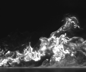
Example instantaneous concentration fields are presented in figure 4(a–c) and the mean concentration and variance fields are presented in figures 4(d) and 4(e), respectively. Intermittent wispy scalar structures are observed similar to those described in the study by Crimaldi & Koseff (Reference Crimaldi and Koseff2001). Subtle discontinuities can be observed in the mean fields between the different fields of view, but are not expected to affect the results and discussions, hence no corrections were applied.

Figure 4. (a–c) Instantaneous concentration fields extracted at  ${t}/({U_{\infty }/\delta })=0.02$ apart with vortical structures trackable across different time frames. Note that each panel is a composite of uncorrelated measurements at P1, P2 and P3, the boundaries of which are denoted by grey lines. (d) Mean concentration and (e) variance fields.
In the near-source region, the scalar is observed to remain close to the ground, and a ‘halo’ glow effect can also be observed at the source where the dye concentration is high. This is present in all instantaneous frames with the same effect showing in the time-averaged (mean) concentration field in figure 4(d). The ‘halo’ glow is non-physical and due to nonlinear secondary fluorescence which has been observed in similar studies (Vanderwel & Tavoularis Reference Vanderwel and Tavoularis2014; Lim et al. Reference Lim, Hertwig, Grylls, Gough, van Reeuwijk, Grimmond and Vanderwel2022) and can introduce a local concentration bias of up to 60 %. Based on figure 4, the ‘halo’ effect does not extend past  $x/\delta \sim 0.5$. Corrections were not applied as this nonlinear effect becomes negligible very quickly farther from the source as the dye concentration decreases.
Far from the source, the scalar field exhibits larger coherent features that can be observed to intermittently extend into the outer layer of the boundary layer in the instantaneous fields. Although the mean concentration is relatively low in the outer layer, the concentration variance map extends farther from the wall than the mean and exhibits distinctive wispy features along the plume boundary due to the increased significance of the rare intermittent events towards the variance than the mean.
4.1. Mean plume characteristics
The dye plume spreads with streamwise distance due to turbulent diffusion. Figure 5 presents the streamwise development of the mean plume's vertical half-width,  $\delta _{y,\bar {C}}$, defined based on the vertical distance from the ground to the half-maximum of the local mean concentration. The self-similar analytical solution for rural flow used by Robins (Reference Robins1978) is also plotted in figure 5. Our results deviated from this, particularly in the near-source region, and a better fit is achieved if a virtual origin is introduced to the analytical solution by shifting the origin downstream, i.e. $x_0=140\,{\rm mm}$ ( $1.3\delta$), and adjusting the scaling constant as
 \begin{equation} \delta_{y,\bar{C}} / \delta = 0.065 \left(\frac{x-x_0}{\delta}\right)^{0.65} . \end{equation}
There are several factors that justify this virtual origin shift from the source location. Firstly, a smooth-wall TBL has a VSL which has a propensity to trap dye (Crimaldi et al. Reference Crimaldi, Wiley and Koseff2002). Robins (Reference Robins1978) had a rough-wall incoming flow and did not have a significant VSL. Secondly, the Schmidt number of the aqueous tracer in this study is  $\textit {O}(10^3)$ which is several orders of magnitude higher than that of the gaseous tracer used by Robins (Reference Robins1978). From Taylor's dispersion theory (Taylor Reference Taylor1922), there are three regimes of diffusion also known as the molecular diffusion, turbulent convection and turbulent diffusion regimes (Castro & Vanderwel Reference Castro and Vanderwel2021). Right at the moment of particle release, dispersion rate is purely due to molecular actions and unaffected by turbulence. Since the molecular diffusion effect is weak in this study, the dye remains trapped in the VSL and the vertical plume growth is low for much longer streamwise distances. The combination of low vertical momentum and low molecular diffusion action removes a ‘catalytic’ mechanism to kick the dye out of the VSL; hence it remains trapped for a longer streamwise distance instead of entering the logarithmic layer very near the source as was observed by Robins (Reference Robins1978). By introducing an origin shift and adjusting the scaling constant, we show that (4.1) is a better description of the mean plume for a smooth-wall TBL application.

Figure 5. Vertical half-width of the plume based on the half-maximum of the mean concentration. The origin in (4.1) is shifted by  $x_0=140$ mm.
A theoretical estimate of  $x_0$ can be derived by considering the advection and diffusion time scales for the scalar to cross the VSL. To estimate the advection time scale, we use $T_u \sim L/U$, where $L$ is the distance from source (i.e. $L \sim x_0$) and $U$ is the advection velocity within the VSL (i.e. $U \sim U_{\tau }$.) The diffusion time scale is estimated as $T_d \sim Y^2 / 8 \gamma$, where $Y$ is the thickness of the VSL (i.e. $y^+ \sim 5$) and $\gamma$ is the molecular diffusivity of Rhodamine 6G in water (i.e. $\gamma =4\times 10^{-10}\,{\rm m}^2\,{\rm s}^{-1}$). By matching the advection and diffusion time scales, we obtained the theoretical maximum limit as: $x_0^{lim} \sim 400\,{\rm mm}$. Our experimental measurement of $x_0$ is slightly smaller than $x_0^{lim}$ due to real-world experimental constraints, but otherwise in good agreement.
Figure 6(a) shows the time-averaged vertical concentration profiles extracted at specific streamwise locations and presented in the self-preserving form based on the analytical gradient transfer theory used by Robins (Reference Robins1978):
 \begin{equation} \frac{\bar{C}}{\overline{C_0}} = \exp\left[-\ln 2\left(\frac{y}{\delta_{y,\bar{C}}}\right)^{1.5}\right], \end{equation}
where  $\overline {C_0}$ represents the mean peak concentration. The profiles are observed to collapse relatively well at approximately $x/\delta >3$. A closer inspection of the profiles shows that $x/\delta >2.7$ (i.e. $(x-x_0)/\delta >1.4$) represents the far field where the plume is fully developed and self-similar. Figure 6(b) presents the streamwise decay of the peak mean concentration. The plume decay rate for $(x-x_0)/\delta >1.4$ scales with a power law according to
 \begin{equation} \frac{\overline{C_0} U_\infty \delta^2}{Q_{dye}C_s} = 50 \left(\frac{x-x_0}{\delta}\right)^{{-}1.39} , \end{equation}
where the power-law exponent of  $-1.39$ is the same as that observed by Robins (Reference Robins1978).

Figure 6. (a) Vertical profiles of the mean concentration and (b) the decay of its peak with streamwise distance.
Equations (4.1), (4.2) and (4.3) are power laws that describe the plume's vertical half-width, vertical profile and peak decay, respectively. Csanady (Reference Csanady1967) showed that these equations can be related using the conservation of mass, but only if the lateral shape of the plume is also known. We observe very similar power-law exponents for the mean concentration and concentration decay in the far field compared with Robins (Reference Robins1978). This provides evidence that the overall plume growth behaviour is similar in the self-similar region, even if the incoming flow conditions of the TBL are slightly different across the two studies. Differences in scaling constants show our plume is slightly wider (in the vertical direction) with lower peak concentrations at the same streamwise distance. We attribute this difference to the presence of a VSL in our study. If we regard the VSL as a dye reservoir releasing dye into the logarithmic layer, molecular diffusion and advection of the dye while it is trapped in the VSL would effectively increase the source size and, thus, reduce the source concentration at this ‘redefined source’.
In comparison with the Gaussian plume model (Arya Reference Arya1999), where both vertical and lateral plume shapes are known, and the plume width grows as  $x^{0.5}$, then conservation of mass requires peak decay to scale as $x^{-1}$. Our results differ from the Gaussian plume model, with the power-law exponents suggesting a relatively faster plume growth and, consequently, faster decay of the peak concentration. These observations are consistent with that of Webster et al. (Reference Webster, Rahman and Dasi2003) who attributed it to non-constant eddy diffusion coefficient. Our results therefore highlight the limitation of the Gaussian plume model in this specific scenario, which relies on the assumption of an isotropic turbulent diffusivity that is uniform in space. We note that there is strong evidence of anisotropic normal- and non-zero cross-diffusivities in various flow applications (Tavoularis & Corrsin Reference Tavoularis and Corrsin1981, Reference Tavoularis and Corrsin1985; Vanderwel & Tavoularis Reference Vanderwel and Tavoularis2014), including smooth-wall TBL flows as we demonstrate later, which explains the departure of our results from the Gaussian plume model.
4.2. Variance of the plume concentration
Accurate prediction of scalar dispersion requires both mean and fluctuating terms to be modelled accurately. Figure 7 presents the streamwise growth of the half-width (similarly, based on the half-maximum) of the concentration variance ( $\delta _{y,\overline {c'c'}}$) compared with the half-width of the mean. The analytical form that best describes the half-width of the variance field is
 \begin{equation} \delta_{y,\overline{c'c'}} / \delta = 0.062 \left(\frac{x-x_1}{\delta}\right)^{0.72}, \end{equation}
with a virtual origin shift of  $x_1 = 30\,{\rm mm}$. The virtual origin shift is required here because the slower release of dye at the near-source region (due to the VSL trapping dye) leads to lower concentration variance. Note that both $x_0$ and $x_1$ are expected to be dependent on $Re$ and $Sc$ since they are linked to the diffusion and advection time scales. Interestingly, the half-width of the variance grows faster than that of the mean concentration. This result deviates from the literature where similar growth rates were observed between the mean concentration and concentration variance (Crimaldi & Koseff Reference Crimaldi and Koseff2006; Vanderwel & Tavoularis Reference Vanderwel and Tavoularis2014), and may possibly be linked to the different boundary conditions across the experiments; this is hypothesised to also have an influence on $x_0$ and $x_1$. Although both curves nearly coincide in the far field, a significant discrepancy exists for $x/\delta <3$. In particular, the half-width of the concentration variance before $x=x_0$ is non-zero. This indicates that in the $x_1< x< x_0$ region where the majority of the dye is still trapped in the VSL, there are intermittent turbulent events that contribute to the vertical transport of the dye. These events are rare and the overall effect of dye transport on the mean concentration is low. As the length scales grow with downstream distance and more dye escapes the VSL, turbulent scalar mixing with the ambient fluid becomes more effective, and hence the growth rates of the half-widths of the mean concentration and concentration variance become similar.

Figure 7. Vertical half-width of the plume based on the half-maximum of the concentration variance. The origin in (4.4) is shifted by  $x_1=30$ mm.
Vertical profiles of the concentration variance are presented in figure 8(a). The collapse of the vertical profiles is achieved using the Weibull function (Brown & Wohletz Reference Brown and Wohletz1995). The resulting equation of best fit is
 \begin{equation} \frac{\overline{c'c'}}{\overline{(c'c')_0}} = 1.9 \left(\frac{y/\delta_{y,\overline{c'c'}}}{0.76}\right)^{0.4} \exp{\left[-\left(\frac{y/\delta_{y,\overline{c'c'}}}{0.76}\right)^{1.4}\right]}, \end{equation}
where  $\overline {(c'c')_0}$ represents the mean peak variance. The best fit describing the decay of the peak concentration variance shown in figure 8(b) is
 \begin{equation} \frac{\overline{(c'c')_0} U_\infty \delta^2}{Q_{dye}C_s^2} = 0.3 \left(\frac{x-x_1}{\delta}\right)^{{-}3.8} . \end{equation}
This follows the same analytical form as (4.3), but the power-law exponent has been adjusted to  $-3.8$ as the variance peak decays much faster. The scaling constant which does not affect the gradient of the line is 0.3.

Figure 8. (a) Vertical profiles of the concentration variance and (b) the decay of its peak with streamwise distance.
To gain greater insights into the concentration variance, the budget for the concentration variance is evaluated. For a steady-state problem with negligible molecular diffusion, the concentration variance follows the transport equation:

where term I represents transport of scalar fluctuations due to advection, term II represents production due to mean concentration gradient, term III represents diffusion due to turbulence, term IV represents diffusion due to molecular motions and term V represents dissipation of fine scales, also known as 2 $\epsilon _c$, where $\epsilon _c$ represents the scalar dissipation rate. All terms are directly measured or calculated from the empirical relations presented earlier, apart from term V as there was no information on $\partial c'/ \partial z$; hence this was calculated using the difference of the other terms.
If we examine the concentration fluctuation transport equation at the wall, the no-slip boundary condition dictates terms I, II and III to be zero. Terms IV and V are processes that do not increase the concentration variance. As such, the concentration variance should theoretically be zero at the wall, which is substantiated by observations from DNS (Hantsis & Piomelli Reference Hantsis and Piomelli2020), and further justifies the Weibull analytical fit in (4.5).
From figure 9, it can be observed that the advection and dissipation terms dominate the concentration fluctuation balance. The signs of these terms are dependent on the signs of their constituent; for example, the advection term is negative because the concentration variance decays with streamwise and wall-normal distance from source. There is also a general decay of all four terms with streamwise distance. At very large  $x/\delta$, the relative magnitude of the production term is expected to increase to values comparable to that of the advection term (Fackrell & Robins Reference Fackrell and Robins1982a).

Figure 9. Concentration fluctuations budget at selected streamwise locations: (a)  $x/\delta = 3.0$, (b) $x/\delta = 4.0$ and (c) $x/\delta = 5.0$. All values are streamwise-median up to $\pm 0.5 x/\delta$ to reduce noise.
The streamwise development of the wall-normal location of the peak of the production term appears to follow  $\delta _{y,\bar {C}}$. This is consistent with the fact that the production term is driven by the mean concentration gradient, which has the largest magnitude close to the half-width as shown in figure 6(a), and that the wall-normal location of its peak scales with $\delta _{y,\bar {C}}$. The wall-normal location of the peak of the diffusion term is not immediately obvious due to the noisy data, but it does appear to be closer to $\delta _{y,\bar {C}}$ than the wall. This is consistent with large-scale turbulence existing in this region as compared with the near-wall region, which is more efficient at transporting the concentration fluctuations.
There is a very subtle change in signs for the production and turbulent diffusion terms at all streamwise locations near the wall ( $y/\delta \sim 0.02$), which has also been observed in the results of Fackrell & Robins (Reference Fackrell and Robins1982a). The sign change for the production term is due to the change in the relative magnitudes of $\overline {c'u'} ({\partial \bar {C}}/{\partial x})$ which is positive and $\overline {c'v'} ({\partial \bar {C}}/{\partial y})$ which is negative. Since the production term is positive very near the wall, it suggests the contribution of $\overline {c'v'} ({\partial \bar {C}}/{\partial y})$ to the production has decreased. We take a closer look into the individual terms of the turbulent scalar fluxes later and return to this point. For the turbulent diffusion term, which is essentially the flux of the variance, Csanady (Reference Csanady1967) suggested this can be represented using a first-order gradient transport model similar to the transport of mean concentration in (1.4). Therefore, a change in sign of the turbulent diffusion term here indicates that there is a change in the gradient of the variance, and at wall-normal locations very close to the wall. This is confirmed in figure 8(a) which shows a concentration variance peak close to the wall.
4.3. Peak-to-mean fields
The concentration peak-to-mean field is an important parameter to consider in applications involving the transport of hazardous materials or pollutants. Figure 10 presents the concentration peak-to-mean map where the peak concentration is defined as the highest local concentration measured throughout the entire acquisition. This definition is useful for applications that need to assess risk if there is an exposure to lethal dosage of hazardous materials. From figure 10, wispy scalar structures above the plume half-width and towards the plume edge can be observed to contain the highest  $C_{peak}/\bar {C}$ ratios. This is a result of highly intermittent scalar structures with thin filaments of high concentrations present in this region, which is consistent with the observations of Crimaldi & Koseff (Reference Crimaldi and Koseff2001). The highest $C_{peak}/\bar {C}$ ratio is found to be close to the source where small-scale scalar structures can be observed, which appear to be relatively ineffective at entraining and mixing the scalar tracer with the ambient flow. As the plume spreads vertically with increasing downstream distance, a larger vertical region of $C_{peak}/\bar {C}>1$ is observed. At the same time, as the plume is advected downstream, molecular diffusion acts to decrease the magnitude of $C_{peak}$. We would expect that for scalars with a higher molecular diffusivity (i.e. smaller Schmidt number), $C_{peak}$ would decrease more quickly and the $C_{peak}/\bar {C}$ ratio would have smaller values.

Figure 10. Concentration peak-to-mean map.
To gain greater insight into the behaviour of the  $C_{peak}/\bar {C}$ ratio across the plume, we examine the p.d.f. of the concentration. Figure 11 presents histograms of the concentration normalised by the concentration fluctuation root-mean-square at 20 selected locations at $x/\delta =1, 2, 3, 4, 5$ and $y/\delta =0.03, 0.05, 0.1, 0.2$. The gamma distribution (Cassiani et al. Reference Cassiani, Bertagni, Marro and Salizzoni2020) fits the histograms of $C/c'_{rms}$ in the plume core, while the lognormal distribution is generally a better fit at the plume edge, as shown in figure 11. In an earlier study of a dispersing plume from an elevated point source, Yee et al. (Reference Yee, Kosteniuk, Chandler, Biltoft and Bowers1993) showed the lognormal distribution is the best fit for short ranges where there is significant plume meandering, while the gamma distribution is the best fit for long ranges where internal structure dominates. There are several phenomenological similarities between the study by Yee et al. (Reference Yee, Kosteniuk, Chandler, Biltoft and Bowers1993) and ours. In our plume edge, the wispy structures contribute to intermittent events with filaments that contain high concentrations, which in terms of contribution to the p.d.f., is similar to the plume meandering effect observed by Yee et al. (Reference Yee, Kosteniuk, Chandler, Biltoft and Bowers1993). In our plume core, the internal structure dominates, which is again similar to the long-range observations by Yee et al. (Reference Yee, Kosteniuk, Chandler, Biltoft and Bowers1993). Hence, the p.d.f. is a function of both streamwise and vertical distance from the wall, and we hypothesise that the lognormal and gamma distributions are the best fit for the plume edge and plume core, respectively, because of the scalar morphology.

Figure 11. Histograms of  $C/c'_{rms}$ at various wall-normal and streamwise locations. Red lines represent gamma and yellow lines represent lognormal fits. Data within four times the average background noise level in the free stream are shaded grey (note that plot (a) is outside of the plume where no significant concentration is measured).
In the study by Fackrell & Robins (Reference Fackrell and Robins1982a), their peak concentration,  $C_{99}$, is defined as the concentration value that is exceeded only 1 % of the time, and they observed $C_{99}/c'_{rms}$ to be insensitive to the source conditions and around 4.5 over most of the plume despite a wide range of concentration fluctuation p.d.f. shapes. Although $C_{99}/c'_{rms}$ is computationally expensive to calculate at every point, in order to facilitate comparisons, we extracted this quantity for the same 19 locations shown in figure 11. A mean value of 4.6 can be observed, which is consistent with the results of Fackrell & Robins (Reference Fackrell and Robins1982a) despite the different scalar Schmidt numbers, and with the predictions by Csanady (Reference Csanady1967) who predicted that this quantity should be between 4.3 and 4.6 based on the assumption that the concentration p.d.f. follows a Poisson distribution. Our measurements show that this quantity is very robust and there appears to be no obvious trend with streamwise or vertical distance even though the concentration peak-to-mean map in figure 10 suggests a strong dependence of the $C_{peak}/\bar {C}$ ratio on spatial location. From these results, we conclude the quantity $C_{99}/c'_{rms} \sim 4.6$ is robust to concentration intermittency levels, concentration p.d.f. shapes and $C_{peak}/\bar {C}$ ratio. The reason behind the rather universal value of $C_{99}/c'_{rms} \sim 4.6$ is because this quantity is defined as the ratio of the right tail of the distribution to its standard deviation. Since many distributions (including Poisson, gamma or lognormal) have similar right tails (at $C_{99}$), this results in a rather universal value for $C_{99}/c'_{rms}$.
5. Concentration–velocity statistics
5.1. Turbulent scalar fluxes
The simultaneous PIV–PLIF measurement technique offers insights into the turbulent scalar fluxes for which very limited previous experimental measurements are available. Figure 12 presents full two-dimensional maps of the mean streamwise and vertical turbulent scalar fluxes, where the directions suggest a net concentration fluctuation transport direction of upward (away from the ground) and to the left (towards the incoming flow). This is reminiscent of Q2 ejection events in TBL flow (Adrian Reference Adrian2007) and we hope to explore this connection in greater detail in a subsequent study. The fluxes are of comparable magnitude because of the correlation between  $u'$ and $v'$, which is inherent in TBLs where Reynolds shear stress is non-zero (see figure 2). In fact, the relative magnitudes of the streamwise and vertical turbulent fluxes also reflect how the magnitude of $\overline {u'u'}$ is about three times larger than that of $\overline {v'v'}$ (see figure 2b,c). In the transport equation of the mean concentration (1.3), ${\rm d}\bar {C}/{\rm d}t$ is dependent on the principal gradients of the fluxes. For the logarithmic region of a TBL, $\partial /\partial x$ scales with $1/l$, where $l$ is the distance from the source, and $\partial /\partial y$ scales with $\delta$. Hence, we expect $\overline {u'c'} / \partial x \ll \partial \overline {v'c'}/\partial y$. Furthermore, since $u' \ll \bar {U}$ and $v' \gg \bar {V}$, we expect $\bar {U} \partial \bar {C}/ \partial x \gg \overline {u'c'} / \partial x$ and $\bar {V} \partial \bar {C}/ \partial y \ll \overline {v'c'} / \partial y$. Therefore, the vertical turbulent scalar flux is much more significant and of greater importance for mathematical or simulation models to capture accurately.

Figure 12. Experimental measurements of the mean (a) streamwise and (b) vertical turbulent scalar fluxes.
Figure 13 presents the vertical profiles of the turbulent scalar fluxes. The far-field plots appear self-similar and collapse relatively well using the half-width of the concentration variance. The near-field plots are not self-similar near the wall, with secondary peaks observed near the ground for locations much smaller than  $x_0^{lim} \sim 400\,{\rm mm}$ because of the trapped dye slowly releasing from the VSL (see figure 13b). We suggest that Weibull-type functions (Brown & Wohletz Reference Brown and Wohletz1995) provide the best fit to the experimental data, as follows:
 \begin{align} \overline{c'u'}/\overline{(c'u')}_0 = 2.25 \left(\frac{y/\delta_{y,\overline{c'c'}}}{0.95}\right)^{0.85} \exp{\left[-\left(\frac{y/\delta_{y,\overline{c'c'}}}{0.95}\right)^{1.85}\right]} , \end{align}
 \begin{align} \overline{c'v'}/\overline{(c'v')}_0 = 2.45 \left(\frac{y/\delta_{y,\overline{c'c'}}}{1.08}\right)^{1.38} \exp{\left[-\left(\frac{y/\delta_{y,\overline{c'c'}}}{1.08}\right)^{2.38}\right]} , \end{align}
where  $\overline {(c'u')}_0$ and $\overline {(c'v')}_0$ represent the peak magnitude of each profile. The Weibull function is a good fit to the data since the derivative of (4.2) would lead to the product of an exponential and a power-law function. However, we note that the empirical coefficients in (5.1) and (5.2) cannot be obtained from the derivative of (4.2) directly as this requires zero cross-diffusivity in the turbulent diffusivity tensor. This is perhaps a limitation of the simple gradient diffusion hypothesis and we further the discussion on turbulent diffusivity in the next section. By using the peaks to normalise the fluxes, this model may overpredict the peak by a factor of up to approximately 1.25.

Figure 13. Vertical profiles of the mean (a) streamwise and (b) vertical turbulent scalar fluxes normalised by their peak.
These equations show that the wall-normal locations of the peak of the turbulent fluxes grow with  $\delta _{y,\overline {c'c'}}$, and that the wall-normal location of the peak of the vertical flux is higher than that of the streamwise flux. The observation of lower magnitudes of the vertical flux relative to the streamwise flux at the near-wall region supports our discussion in § 4.2 where we observed a change in sign of the production term of the concentration variance and attributed it to the relative magnitudes of the turbulent fluxes.
Figure 14 presents the streamwise decays of the peaks of the turbulent scalar fluxes, where the region  $(x-x_1)/\delta >0.45$ can be described by the following power laws:
 \begin{align} \frac{\overline{(c'u')}_0}{C_s U_\infty} ={-}5 \times 10^{{-}5} \times \left(\frac{x-x_1}{\delta}\right)^{{-}1.6} , \end{align}
 \begin{align} \frac{\overline{(c'v')}_0}{C_s U_\infty} = 1.6 \times 10^{{-}5} \times \left(\frac{x-x_1}{\delta}\right)^{{-}1.6} . \end{align}
The virtual origin shifts in these equations mirror that of the decay of the peak concentration variance in (4.6) instead of the mean concentration in (4.3). This is because at the near-source region, the observation of mean concentration (or a lack of) is the direct observation of a physical phenomenon where dye is trapped in the VSL. In contrast, the turbulent scalar fluxes (similar to concentration variance) describe the mechanism of the scalar transport due to turbulence, which will only approach zero towards the VSL where Reynolds stresses also go to zero. With a slower release of dye at the near-source region due to the VSL trapping dye, this leads to lower concentration variance, and hence we hypothesise that a shift in virtual origin for the turbulent fluxes which mirrors that of the decay of the peak concentration variance is necessary. Thus, (5.3) and (5.4) are shifted by  $x_1$.

Figure 14. Decay of the peak of the mean (a) streamwise and (b) vertical turbulent scalar fluxes.
Csanady (Reference Csanady1967) showed that the only condition for self-similarity is that the variation of the decay time scale of the concentration fluctuation with distance from source is self-similar. Since the decay of the turbulent scalar fluxes presented here (and concentration variance in figure 8b) has achieved self-similarity before the mean plume concentration, and that the mean concentration also contains information on the secondary peaks near the ground due to the VSL slowly releasing dye, it can be concluded that the self-similarity of the mean concentration is a sufficient criteria to accurately predict self-similar turbulent scalar fluxes and concentration variance.
5.2. Turbulent diffusivity
The turbulent diffusivity tensor (see (1.4)) relates the turbulent scalar fluxes to the mean concentration gradient and offers insights into the contribution of the concentration gradients to the turbulent scalar fluxes. In the centre-plane of the plume, where our data are measured, the contributions of the individual components of the tensor to the turbulent scalar fluxes can be decomposed as


where the spanwise concentration derivatives are zero due to symmetry about the  $xy$ plane.
To calculate the individual components of the turbulent diffusivity tensor, the mean concentration gradient and turbulent scalar fluxes are required. Numerical differentiation of the concentration field from the raw experimental dataset would result in very noisy concentration gradient fields; hence we used the empirical equations describing the concentration plume in (4.1), (4.2) and (4.3), which are valid for a fully developed and self-similar plume ( $x/\delta >2.7$), to calculate the concentration gradients by analytical differentiation. The analytical concentration gradient maps are presented in figure 15. It can be observed that the sign of the streamwise concentration gradient changes with distance from the wall. Negative values near the wall are expected when the sampling point is within the plume and the concentration decays with streamwise distance. Away from the wall and near the plume edge, the growth of the plume results in an increase in concentration with streamwise distance. The vertical concentration gradient remains negative throughout the entire map as the concentration decreases monotonically with distance from the wall.

Figure 15. Mean (a) streamwise and (b) vertical concentration gradients calculated using analytical differentiation. Region that is not self-similar with the empirical relations is shaded grey.
Before solving for the turbulent diffusivity tensor, consider that with four unknowns in  $D_{xx}$, $D_{xy}$, $D_{yx}$ and $D_{yy}$ and two equations in (5.5) and (5.6), this is still an underdetermined system. To circumvent this problem, we introduce an additional constraint which assumes $\boldsymbol{\mathsf{D}}_{ij}$ varies smoothly and gradually in space. Without making a priori assumptions of the shape of $\boldsymbol{\mathsf{D}}_{ij}$, we regularise the problem by applying an $11 \times 11$ (i.e. $0.9\,{\rm mm} \times 0.9\,{\rm mm}$) moving window, where $\boldsymbol{\mathsf{D}}_{ij}$ is assumed to be constant within. The window size is selected based on two considerations: it has to be larger than the PIV vector resolution (0.51 mm), but not too large as it will over-smooth the solutions. Each window leads to an overdetermined system which is then solved using Matlab's QR factorisation solver.
Figure 16 presents the individual components of the resulting turbulent diffusivity tensor. The maps are considerably noisier towards the edge of the plume which can be attributed to higher dye intermittency resulting in fewer scalar events that contain relatively high concentration, consistent with the concentration peak-to-mean map shown in figure 10, and consequently low mean concentration gradients. Due to the noisy results at higher vertical distances, we focus our attention on just  $y/\delta <0.4$. In this region, the turbulent diffusivity can be observed to be relatively invariant to streamwise distance. Some notable conclusions are:
(i) Component $D_{yy}$ is essentially positive everywhere, confirming that vertical transport correlates well with the vertical concentration gradient.
(ii) Component
$D_{xy}$ is negative, indicating that the vertical concentration gradients result in upstream turbulent transport. This is a consequence of the negative Reynolds shear stress present in TBL, which results from the anti-correlation of $u'$ and $v'$, and could be attributed to Q2-type ejection events.(iii) Both
$D_{xx}$ and $D_{yx}$ change sign with wall-normal distance. This reflects the change in sign of ${\rm d}\bar {C}/{{\rm d}\kern0.7pt x}$ observed in figure 15. In addition, these two components appear to have opposite sign, which again is a consequence of the anti-correlation of $u'$ and $v'$. Although the measurements of these components exhibit the most noise, we show below that they contribute the least to the net transport.


Figure 16. Streamwise-median ( $2.7 < x/\delta < 5.57$) profiles and maps of the turbulent diffusivity components: (a) $D_{xx}$, (b) $D_{xy}$, (c) $D_{yx}$ and (d) $D_{yy}$. The (shading) bounds of the profiles represent one standard deviation of the streamwise variations of the map. Values above 4.8 $\delta _{y,\bar {C}}$ are discarded in the maps.
In order to appreciate the significance of each component of the turbulent diffusivity tensor, figure 17 shows how each component contributes to the net turbulent scalar fluxes at three downstream locations. It is clear from figure 17(a) that the  $D_{xy}$ component provides the dominant contribution to the net streamwise flux $\overline {c'u'}$, despite the magnitude of $D_{xx}$ being greater than that of $D_{xy}$. It is also clear from figure 17(b) that the $D_{yy}$ component provides the dominant contribution to the net vertical flux $\overline {c'v'}$, with the $D_{yx}$ component having almost negligible influence.

Figure 17. (a,b) Contributions of the concentration gradients to the turbulent scalar fluxes at streamwise locations (i)  $x/\delta =3.0$, (ii) $x/\delta =4.0$ and (iii) $x/\delta =5.0$. Here $\boldsymbol{\mathsf{D}}_{ij}$ and $K$ are streamwise-median over $\pm 0.5x/\delta$ to reduce noise; turbulent fluxes and analytical concentration gradients are extracted at specified locations.
This leads us to an alternative approach, which is to approximate an effective turbulent diffusivity coefficient  $K$ that can be used to describe the vertical turbulent transport. This approach assumes that the orthogonal components of the concentration gradient do not contribute to the turbulent scalar fluxes, and therefore the vertical turbulent scalar flux is driven only by the vertical concentration gradient. The effective turbulent diffusivity coefficient is then obtained directly as
 \begin{equation} K= \frac{-\overline{c'v'}}{{{\rm d}\bar{C}}/{{\rm d}y}} . \end{equation}
The variation of the resulting  $K$ is included in figure 17(b) and it is clear that it very closely resembles $D_{yy}$, confirming that vertical turbulent transport is described well by this simple gradient transport model.
5.3. Turbulent Schmidt number
The turbulent Schmidt number is a useful way of comparing the magnitude of the turbulent diffusivity with the turbulent viscosity. In order to make this comparison, figure 18(a) compares  $D_{yy}$, the dominant component of the turbulent diffusivity tensor, and $K$ the effective turbulent diffusivity coefficient, with the turbulent viscosity determined in § 3 (figure 2e). Recall that the discrepancy between $D_{yy}$ and $K$ is due to the anisotropic components of the turbulent diffusivity tensor, which appear less negligible near the wall. The plot shows that all values tend to zero near the wall, and grow with wall-normal distance at similar rate; however, the turbulent viscosity tends to a different value farther away from the wall.

Figure 18. (a) Comparison of the streamwise-median ( $2.7 < x/\delta < 5.57$) turbulent viscosity $\nu _t$ with the turbulent diffusivity obtained using two methods: as $D_{yy}$, the dominant component of the turbulent diffusivity tensor, and as $K$, the effective turbulent diffusivity coefficient. (b) The streamwise-median ( $2.7 < x/\delta < 5.57$) turbulent Schmidt number, i.e. the ratio of the turbulent viscosity and the turbulent diffusivity, based on $D_{yy}$ and on $K$.
$K$.
The ratios of the streamwise-averaged profile of the turbulent viscosity and diffusivities are presented in figure 18(b) to give an estimate of the appropriate value of turbulent Schmidt number. We observe good agreement for  $y/\delta > 0.14$. Close to the wall, the values predicted by $D_{yy}$ go to zero while values predicted by $K$ do not. The streamwise concentration gradient acts as an impedance to the vertical scalar fluxes and has a larger influence in the near-wall region (see also figure 17). The assumption of only principal components of the concentration gradient contributing to the turbulent scalar fluxes is valid for $y/\delta > 0.14$.
The turbulent Schmidt number calculated using the turbulent viscosity and  $D_{yy}$ is presented in figure 19. The streamwise-median profile is preferred over streamwise-averaging to reduce the influence of noise skewing the profile in the outer layer. Far from the wall (e.g. see $y/\delta =0.5$), the results are nonetheless noisy which can be attributed to a general lack of scalar events; hence our analysis focuses on the region from the wall to approximately $y/\delta =0.4$. The streamwise-median profile exhibits the same shape as that observed by Koeltzsch (Reference Koeltzsch2000), with values going to zero at the wall, but with the peak at around $y/\delta =0.2$ rather than $y/\delta =0.3$. The peak value is approximately 1.25 at the edge of the logarithmic region of the boundary layer. This peak remains consistent, and its value as well as the profile below it do not change with streamwise distance from source.

Figure 19. Streamwise-median profile (black) and the corresponding map of the turbulent Schmidt number calculated using the turbulent viscosity and  $D_{yy}$. Profiles extracted at specified streamwise locations (coloured) are streamwise-median over $\pm 0.5x/\delta$ to reduce noise.
In the near-wall region, since viscosity effects are expected to dominate, the observation of  $Sc_t$ approaching zero is reasonable and agrees with previous studies of similar point-source conditions (Koeltzsch Reference Koeltzsch2000). In the logarithmic region where $Sc_t > 1$, this suggests a reluctance of the dye (relative to momentum) to be transported by the flow structures. To understand this, we refer to an earlier study involving dye released in uniformly sheared flow (Vanderwel & Tavoularis Reference Vanderwel and Tavoularis2016), where dye was observed to segregate preferentially within vortex cores and unlikely to be at the periphery of the vortex. There are two ways to interpret this, depending on distance to the wall. Close to the wall, dye is more likely to exist in bulk quantities (see figure 4) as compared with the length scale of the flow vortices, and hence the preferential segregation of dye would not matter. Away from the wall, since dye is intermittent and sparse, the preferential segregation of dye becomes an important factor to consider in every vortex–dye interaction event. This acts as an impedance to scalar transport statistically which results in $Sc_t > 1$.
6. Conclusions
In this study, the dispersion of a plume from an isokinetic ground-level point source in a canonical smooth-wall TBL is experimentally investigated in a water flume facility using simultaneous PIV and PLIF techniques. In the far field, the half-width, vertical profiles and peak decay of the mean concentration and concentration variance exhibit self-similar behaviour and are collapsed using empirical relations similar to those proposed by Robins (Reference Robins1978). In the near-source region, the plume half-width remains relatively constant due to the lack of a ‘catalytic’ mechanism (i.e. low vertical momentum and molecular diffusion) that can kick the dye out of the VSL into the logarithmic layer. The concentration histograms suggest rapid small-scale mixing dominating the near-source region, while in the far field, large-scale scalar mixing transports dye away from the ground and towards the plume edge where rapid small-scale mixing occurs. The concentration peak-to-mean maps show that the mean can underestimate the peak by up to 50 times, and that these maximum peak ratios occur at vertical distances close to the plume edge.
For the first time, full two-dimensional maps of the turbulent scalar fluxes are presented in a plane aligned with the centreline of the ground source plume. The turbulent scalar fluxes show a net transport direction of upward and towards the incoming flow. Vertical profiles of the turbulent scalar fluxes are shown to collapse well with Weibull-type exponential functions while their peak decays follow power laws. Four components of the anisotropic turbulent diffusivity tensor  $\boldsymbol{\mathsf{D}}_{ij}$ are calculated, along with an effective turbulent diffusivity coefficient $K$. Both methods show that the turbulent diffusivity is roughly homogeneous in the streamwise direction but varies with wall-normal direction. The vertical concentration gradient is observed to drive the dominant component of turbulent transport in both streamwise and vertical turbulent scalar fluxes, while the streamwise concentration gradient slightly reduces the magnitude of the turbulent scalar fluxes.
The magnitudes of the dominant turbulent diffusivity tensor component  $D_{yy}$ and the effective turbulent diffusivity coefficient $K$ compare well with the turbulent viscosity $\nu _t$, calculated via Boussinesq's hypothesis from the Reynolds stress and the velocity gradient. The streamwise-median profile of the turbulent Schmidt number agrees with the trend observed by Koeltzsch (Reference Koeltzsch2000) where values vary with wall-normal distance. A peak value of 1.25 was observed at the edge of the logarithmic layer. Values above unity indicate a reluctance of dye being transported by flow structures. One interpretation of this is the preferential segregation of dye within vortex cores as observed in an earlier study (Vanderwel & Tavoularis Reference Vanderwel and Tavoularis2016). We hope to further explore the relationship between the flow structures and dye transport in future studies.
Acknowledgements
The critical comments and suggestions by four anonymous referees helped to improve the paper.
Funding
The authors gratefully acknowledge the support of C.V.'s UKRI Future Leader's Fellowship (MR/S015566/1) and H.D.L.'s Royal Academy of Engineering Intelligence Community Postdoctoral Research Fellowship (ICRF2122-5-184).
Declaration of interests
The authors report no conflict of interest.
Data availability statement
The data that support the findings of this study are openly available in the University of Southampton repository at https://doi.org/10.5258/SOTON/D2706, reference number 131755347.


 Open access