


1. Introduction
Thermally expanding and contracting flows are found in many fields and engineering applications that deal with heat transfer to a fluid, such as chemical reactors, energy systems and propulsion systems. If a gas is heated or cooled, its density changes. In internal flows this leads to acceleration or deceleration, respectively. Consequently the flow is subjected to two different effects which differentiate them from the well-studied fully developed incompressible wall bounded flows. Firstly, the flow experiences a favourable or adverse pressure gradient that causes the bulk velocity to change along the streamwise direction. Secondly, local property variations affect turbulence by modifying momentum transfer through variable inertia effects (Lele Reference Lele1994).
Accelerating and decelerating flows have been studied extensively in the context of incompressible turbulence. Extensive knowledge has been gathered mainly through the analysis of adverse and favourable pressure gradient (FPG) boundary layers. Piomelli, Balaras & Pascarelli (Reference Piomelli, Balaras and Pascarelli2000) and Piomelli & Yuan (Reference Piomelli and Yuan2013) studied spatially developing accelerated boundary layers and showed that, for accelerated boundary layers, the skin friction coefficient decreases while the logarithmic layer disappears, replaced by a well-mixed region which tends to decrease turbulent production. The latter reflects the well known tendency of a flow to relaminarize if subjected to strong acceleration. They also noticed a steep increase in anisotropy in the accelerated region with  $v^{\prime }$ and $w^{\prime }$ becoming almost negligible as turbulence tends to the one-dimensional limit. Bobke et al. (Reference Bobke, Vinuesa, Örlü and Schlatter2017), on the other hand, presents a detailed account on the effects of adverse pressure gradients in boundary layers. They report a larger velocity-pressure gradient correlation in the buffer region and more energized large-scale structures when compared with corresponding zero pressure gradient boundary layers at the same friction Reynolds number. More recently, Bross, Fuchs & Käler (Reference Bross, Fuchs and Käler2019) used adverse pressure gradients to enhance the probability of reverse-flow events which are particularly rare in zero pressure gradient boundary layers.
On the other hand, most of the knowledge on turbulence modulation by variable properties in wall turbulence has been gathered in the framework of fully developed flows, such as supersonic boundary layers (Spina & Smits Reference Spina and Smits1987; Pirozzoli, Bernardini & Grasso Reference Pirozzoli, Bernardini and Grasso2008; Ringuette, Wu & Martin Reference Ringuette, Wu and Martin2008; Pirozzoli & Bernardini Reference Pirozzoli and Bernardini2011) and turbulent channel flows (Foysi, Sarkar & Friedrich Reference Foysi, Sarkar and Friedrich2004; Zonta, Marchioli & Soldati Reference Zonta, Marchioli and Soldati2012; Patel et al. Reference Patel, Peeters, Boersma and Pecnik2015; Patel, Boersma & Pecnik Reference Patel, Boersma and Pecnik2016; Sciacovelli, Cinnella & Gloerfelt Reference Sciacovelli, Cinnella and Gloerfelt2017). In his early work Morkovin (Reference Morkovin1961) reported that in a compressible flow, property fluctuations can be neglected as turbulence modulation occurs mainly due to mean property variations. Based on this hypothesis, Huang, Coleman & Bradshaw (Reference Huang, Coleman and Bradshaw1995) suggested a semilocal scaling to account for local property variations, which was successfully used by Trettel & Larsson (Reference Trettel and Larsson2016) and Patel et al. (Reference Patel, Boersma and Pecnik2016) to characterize variable property turbulence. Foysi et al. (Reference Foysi, Sarkar and Friedrich2004), on the other hand, showed that, while semilocal scaling can account for the variations of mean quantities, it is not well suited to study pressure fluctuations and pressure effects, as these are related to non-local interactions.
Large accelerations caused by gas heating in pipe flows has also been investigated extensively, mostly with the aim to characterize flow relaminarization and the consequent heat transfer deterioration. Early studies, including the work of Bankston (Reference Bankston1970), McEligot, Coon & Perkins (Reference McEligot, Coon and Perkins1970) and McEligot, Coon & Perkins (Reference McEligot, Coon and Perkins1982), show the tendency of a heated flow to laminarize when subjected to large heat fluxes. The same result has been confirmed through high fidelity direct numerical simulations (DNS) in later years (Bae, Yoo & Choi Reference Bae, Yoo and Choi2005; Nemati et al. Reference Nemati, Patel, Boersma and Pecnik2015). It has been shown that acceleration tends to decrease turbulent production which leads to lower turbulence intensities (Kline et al. Reference Kline, Reynolds, Schraub and Runstadler1967). Moreover, in fluids with large property variations (Bae et al. Reference Bae, Yoo, Choi and McEligot2006; Nemati Reference Nemati2016) in vertical pipe flows, the main contributor to the laminarization is a combination of buoyant forces and variable inertia effects. The strong role of buoyancy has been confirmed by He & Seddighi (Reference He, He and Seddighi2016) who studied the laminarization of flows subjected to streamwise body forces. Although these investigations show the effect of thermal expansion, no work has been done to reconcile the variable property effects to the streamwise acceleration effect as all the aforementioned studies focused more on the heat transfer process and the similarities between velocity and temperature profiles.
For this reason, in our study, we investigate developing cases with different properties, to assess and distinguish the influence of variable property effects and streamwise acceleration and deceleration. Buoyancy is neglected (assuming horizontal flow) to pinpoint the impact of acceleration/deceleration. Different constitutive laws for viscosity enable us to simulate different fluid responses to thermal expansion and contraction. In particular, we will make extensive use of the semilocal scaling framework, to contextualize streamwise acceleration/deceleration in variable property flows.
2. Numerical details and case descriptions
In the present work we consider flows in the low Mach number limit, such that the low Mach number approximation of the Navier–Stokes equations can be employed. With this assumption, the thermodynamic pressure is considered constant and the hydrodynamic pressure is determined from the mass conservation (Majda & Sethian Reference Majda and Sethian1985). As a consequence the compressibility effects associated with density changes because of pressure variations are neglected. This assumption is realistic in cases of high temperatures and atmospheric pressures gases in which the speed of sound tends to be high, such as hot water vapour or carbon dioxide. The governing equations thus read
 $$\begin{gather} \frac{\partial \rho}{\partial t} + \frac{ \partial \rho u_j}{\partial x_j} = 0 , \end{gather}$$
 $$\begin{gather}\frac{\partial \rho u_i}{\partial x_j} + \frac{\partial \rho u_i u_j}{\partial x_j} ={-} \frac{ \partial p}{\partial x_i} + \frac{1}{Re_0} \frac{\partial }{\partial x_j}\left[ \mu \left( \frac{\partial u_i}{\partial x_j} + \frac{\partial u_j}{\partial x_i} \right) - \frac{2}{3}\mu\frac{\partial u_k}{\partial x_k} \delta_{ij} \right] , \end{gather}$$
 $$\begin{gather}\frac{\partial \rho H}{\partial x_j} + \frac{\partial \rho H u_j}{\partial x_j} = \frac{1}{Re_0 Pr_0} \frac{\partial }{\partial x_j} \left( \frac{\lambda}{c_p} \frac{\partial H}{\partial x_j} \right) . \end{gather}$$
Here  $\rho ,\boldsymbol {u}$ and $H$ are non-dimensional density, velocity vector and enthalpy, respectively, while $t, \boldsymbol {x}, p , \mu , \lambda$ and $c_p$ are non-dimensional time coordinate, spatial direction vector, pressure, viscosity, thermal conductivity and specific isobaric heat capacity, respectively. The constitutive relations for the thermophysical properties ( $\rho , \mu , \lambda , c_p$) as functions of temperature will be detailed later. The non-dimensional variables are defined as
 \begin{equation} \left.\begin{gathered} t = \frac{t^{*} h^{*}}{u_{\tau 0}^{*}}, \quad \boldsymbol{x} = \frac{\boldsymbol{x}^{*}}{h^{*}}, \quad \rho = \frac{\rho^{*}}{\rho^{*}_0}, \quad \mu = \frac{\mu^{*}}{\mu^{*}_0}, \quad \lambda=\frac{\lambda^{*}}{\lambda^{*}_0}, \\ \boldsymbol{u} = \frac{\boldsymbol{u}^{*}}{u^{*}_{\tau 0}}, \quad c_p = \frac{c_p^{*}}{c_{p0}^{*}}, \quad p = \frac{p^{*}}{\rho^{*}_0 {u^{*}_{\tau 0}}^{2}}, \quad H = \frac{H^{*} - H^{*}_0}{c_{p0}^{*} T^{*}_0}, \end{gathered}\right\} \end{equation}
where  $h^{*}$ is the half-channel height and $u^{*}_{\tau }$ is the wall friction velocity. The asterisk identifies a dimensional value, while the subscript $0$ denotes inlet values. The non-dimensional parameters are defined as follows: (i) Reynolds number $Re_{\tau 0} = \rho ^{*}_0 u_{\tau 0}^{*} h^{*} / \mu _0^{*}$; (ii) Prandtl number $Pr_0 = c^{*}_{p0} \mu ^{*}_0 / \lambda _0^{*}$. The solution of equations (2.1a)–(2.1c) is obtained by employing a DNS code which has extensively been validated in Nemati et al. (Reference Nemati, Patel, Boersma and Pecnik2015). The Navier–Stokes equations are discretized with a fully staggered second-order central discretization scheme in space, and a second-order Adams–Bashforth scheme developed by Najm, Wyckoff & Knio (Reference Najm, Wyckoff and Knio1998) in time. This particular scheme is chosen to tackle the instability caused by high density gradients. In addition, a Koren slope limiter is used for the convective fluxes in the enthalpy equation (2.1c). In both substeps of the Najm time discretization scheme, the Poisson equation is solved using fast Fourier transforms in the streamwise and spanwise directions and a second-order discretization in the wall-normal direction. At the outlet, a convective boundary condition is used, while at the inlet the values for velocity are prescribed from an auxiliary fully developed isothermal DNS simulation. Figure 1 shows the method adopted to obtain the inlet conditions for the thermally developing channel. The fully developed isothermal DNS has the same grid resolution (in all three directions) and time step as the thermally developing channel but one third of the length in the streamwise direction ( $L_x = 4{\rm \pi} h^{*}$). The length in the spanwise and wall-normal direction is the same for the isothermal and developing simulations. The midplane of the auxiliary isothermal simulation is fed directly and continuously to the inlet of the developing simulation. For the validation of the DNS code, the reader is referred to Nemati et al. (Reference Nemati, Patel, Boersma and Pecnik2015). The results are analysed in terms of Reynolds average and fluctuations (denoted by the symbols $\bar {\bullet }$ and $\bullet '$, respectively) and Favre average and fluctuations (represented by $\tilde {\bullet }$ and $\bullet ''$, respectively).

Figure 1. Schematic showing the set-up for the developing simulations. The left channel is an auxiliary isothermal periodic DNS which feeds the fully developed inlet to the developing simulation. Note that the heating/cooling of the wall in the thermally developing simulation is introduced at  $x/h=0.82$.
Five cases have been simulated and are detailed in table 1. The database comprises of a mix of accelerating and decelerating cases. The accelerating cases (indicated by A) have an inlet temperature of 500 K, while the isothermal wall temperature is 1170 K. The decelerating cases (denoted by D) enter the domain at 1000 K while the isothermal walls are kept at 660 K. For all cases, density is calculated as density of water vapour at 1 bar, which is tabulated as a function of temperature using the Reference Fluid Thermodynamic and Transport Properties database (REFPROP) (Lemmon et al. Reference Lemmon, Bell, Huber and McLinden2018). It is worth mentioning that due to the high temperatures considered in this study, the density behaviour is practically indistinguishable from the ideal gas law. This leads to a density at the wall which is 0.42 times lower than at the inlet for the accelerating cases and 1.51 times higher than at the inlet for the decelerating cases. The thermal conductivity is also tabulated from REFPROP as a function of temperature. The constitutive law for dynamic viscosity, on the other hand, has been varied to achieve the desired conditions of interest. In particular, for the entries denoted with  $\textrm {H}_2\textrm {O}$ in table 1, the viscosity follows values for water vapour obtained by REFPROP; the simulation denoted with $\textrm {C}\mu$ has a constant viscosity throughout the channel, while for the cases denoted with $\textrm {C}Re^{\star }_\tau$, the viscosity is proportional to density as $\mu /\mu _0 = \sqrt {\rho /\rho _0}$ (as in Patel et al. (Reference Patel, Peeters, Boersma and Pecnik2015)) to maintain a constant semilocal Reynolds number ( $Re_\tau ^{\star }$) along the channel height. All properties tabulated from REFPROP have been discretized on a 2000 point grid in the temperature range $T = [500,1800]$ K, and retrieved via a cubic spline interpolation procedure.
Table 1. Simulated cases. A stands for accelerating (heated) and D stands for decelerating (cooled). The acronym after the hyphen indicates the constitutive relation of viscosity as function of temperature. Symbols for the different cases will be consistent in all plots and further sections (note that the black dashed–dotted line represents the isothermal DNS at  $Re_\tau =547$).

The evolution of bulk quantities in the streamwise direction is shown in figure 2. Bulk velocity increases for the heated cases and decreases for cooled cases. Note that  $\rho _b$ and $T_b$ are not shown ( $\rho _b = U_{b0} U_b^{-1}$ and $T_b \sim \rho _b^{-1}$). The evolution of bulk viscosity is inversely proportional to the bulk Reynolds number $Re_b$.

Figure 2. Streamwise evolution of bulk quantities: (a) velocity; (b) viscosity; (c) thermal conductivity. The dashed red line is for case A-H $_2$O, the dotted red line for case A-C $\mu$, the solid red line for case A-C $Re^{\star }_\tau$, the dashed blue line for case D-H $_2$O and the solid blue line for case D-C $Re^{\star }_\tau$.
Figure 3 presents the evolution of non-dimensional parameters  $Re_\tau$ and $Pr_w$. In terms of friction Reynolds number ( $Re_\tau$) it is possible to notice a steep gradient across the thermal boundary condition step change. In particular, $Re_\tau$ decreases for the heated cases and increases for the cooled cases. While for the realistic cases (A-H $_2$O and D-H $_2$O) $Re_\tau$ follows the same trend of $Re_{b}$, for cases A-C $Re^{\star }_\tau$ and D-C $Re^{\star }_\tau$, $Re_\tau$ is inversely proportional to $Re_b$. The cases with $\textrm {H}_2\textrm {O}$-like varying viscosity exhibit the largest difference, with $Re_\tau$ reaching a value of around 150 for A-H $_2$O and 1040 for D-H $_2$O. The cases with viscosity varying as $\sqrt {\rho }$ have a more moderate Reynolds number change, as this is modified only by a change in wall shear stress, resulting in an outlet $Re_\tau$ equal to 430 and 585 for A-C $Re^{\star }_\tau$ and D-C $Re^{\star }_\tau$, respectively. Finally, the heated case with constant viscosity experiences a mild decrease of $Re_\tau$ upon heating from the walls, reaching a final value of around 315. Figure 3 is complemented with the semilocal Reynolds number $Re_{\tau }^{\star }$ at the outlet, defined as $Re_\tau ^{\star } = \bar {\rho } u_\tau ^{\star } h/\bar {\mu }$, where $u_\tau ^{\star } = \sqrt {\tau _w/\bar {\rho }}$ is the semilocal friction velocity and $\tau _w$ is the wall shear stress. This parameter has proved to be good at describing the influence of variable property flows in fully developed variable property turbulence (i.e. with no streamwise evolution) (Patel et al. Reference Patel, Peeters, Boersma and Pecnik2015, Reference Patel, Boersma and Pecnik2016).

Figure 3. (a) Streamwise evolution of friction Reynolds number  $Re_\tau$. (b) Semilocal Reynolds number plotted against wall-normal coordinate at the channel outlet. (c) Streamwise evolution of wall Prandtl number $Pr_w$. Lines as in figure 2. The vertical dashed line in panels (a,c) indicates the streamwise location of the step change in thermal boundary conditions, from adiabatic to the prescribed wall temperature ( $x/h = 0.82$). In panel (b), the black dashed–dotted line shows the inlet value.
Finally, figure 3(c) shows the Prandtl number based on wall values. The changes in Prandtl number follow an opposite trend with respect to  $Re_\tau$. The largest change is experienced by cases with viscosity varying as $\sqrt {\rho }$. For the cases A-H $_2$O and D-H $_2$O, the changes in viscosity and thermal conductivity balance each other causing the Prandtl number to hardly change with streamwise position.
In terms of the computational grid, the mesh employed is the same for all the simulations and comprises of  $2304\times 408\times 576$ grid points in the streamwise, wall-normal and spanwise directions, for a box size of $12 {\rm \pi}\times 2 \times 2 {\rm \pi}$. The grid resolution is shown, normalized by the Kolmogorov length scales, in figure 4.

Figure 4. Grid resolution normalized by Kolmogorov length scales as a function of  $y^{+}_0$ at the inlet (dashed–dotted line) and at the end of the channel ( $x/h=35$).
3. Streamwise evolution of velocity
Figure 5 shows the averaged streamwise velocity profiles at different streamwise locations ( $x/h = 1.2$, 7.5, 15 and $35$) plotted against the inlet $y^{+}$ coordinate. While the changes in the viscous sublayer occur extremely rapidly after the location where the heating or cooling begins, the log layer continues evolving in the streamwise direction for all the cases. If the changes in the velocity profiles are solely a product of variable property turbulence, it is possible to re-plot $u$ in terms of the semilocal coordinate $y^{\star } = y {Re}_{\tau }^{\star }/h$, by using a transformation developed by Patel et al. (Reference Patel, Peeters, Boersma and Pecnik2015),
 \begin{equation} \bar{u}^{{\star}}(y^{{\star}}) = \int_0^{y^{{\star}}} \frac{\bar{\tau}_{xy}}{\tau_w} {\textrm{d} y}^{{\star}}, \end{equation}
where  $\bar {\tau }_{xy}$ is the mean tangential viscous shear stress and $\tau _w$ is the wall shear stress. Patel et al. (Reference Patel, Peeters, Boersma and Pecnik2015) and Trettel & Larsson (Reference Trettel and Larsson2016) showed that, if the Morkovin hypothesis is satisfied, in fully developed channel flows this transformation yields a universal velocity profile, collapsing velocity profiles for flows characterized by different property variations. This is akin to claiming that viscous shear stress, in fully developed turbulent channel flows, scales with local mean properties. By using $\bar {u}^{\star }$ we can identify the effects of thermal expansion and contraction and isolate them from the influence of fully developed or ‘equilibrium’ property gradients effects. By equilibrium property gradients effects we denote the compressibility effects which are caused by average property gradients in the wall-normal direction only (Foysi et al. Reference Foysi, Sarkar and Friedrich2004; Zonta et al. Reference Zonta, Marchioli and Soldati2012; Pei et al. Reference Pei, Chen, Hussain and She2013; Patel et al. Reference Patel, Peeters, Boersma and Pecnik2015, Reference Patel, Boersma and Pecnik2016).

Figure 5. Streamwise velocity normalized by inlet friction velocity along the inlet  $y^{+}$ at different streamwise locations. Lines as in figure 3. The black dashed–dotted line shows the isothermal inlet.
Figure 6 shows the  $\bar {u}^{\star }$ profiles at the same streamwise location as in figure 5. Three observations can be made. First, the excellent collapse obtained in the viscous sublayer ( $y^{\star }<10$) suggests that the differences found in the viscous-dominated region of the $\bar {u}$ profile are mainly a consequence of local averaged properties. Second, the buffer and log-law region exhibit various differences between the cases. Contrarily to the viscous sublayer, this hints at a modulation of turbulent structures due to predominantly non-local effects. In general, heated cases (red) show a higher log-law constant than the fully developed inlet profile, while case D-H $_2$O has a lower log-law constant. Case D-C $Re^{\star }_\tau$ does not deviate from the isothermal inlet throughout the whole extent of the developing domain. It is worth mentioning that, due to the chosen boundary conditions, the magnitude of the deceleration in the cooled cases is much lower than the acceleration felt by the heated cases (see figure 2). Finally, the deviation for cases A-C $\mu$ and A-C $Re^{\star }_\tau$ (beyond a certain streamwise location) is somewhat larger than for case A-H $_2$O. The same can be concluded about D-H $_2$O when compared with D-C $Re^{\star }_\tau$.

Figure 6. semilocal transformed streamwise velocity along  $y^{\star }$ at different streamwise locations. Lines as in figure 3. The black dashed–dotted line shows the isothermal inlet.
Figure 7 shows a comparison of velocity profiles at different streamwise locations. Figure 7(a–d) shows the un-scaled velocity profile, while figure 7(e–h) shows the velocity transformed according to (3.1). It is possible to notice that, while the Reynolds averaged velocity profiles evolve continuously moving downstream (i.e. increases for accelerating cases and decreases for decelerating),  $\bar {u}^{\star }$ collapses reasonably above $x/h>9$. This suggests that the spatial evolution of the velocity profiles, beyond a certain streamwise location, can be accounted for by local effects only, e.g. characterized by $Re_{\tau }^{\star }$. As such, the channels can be considered ‘quasi-homogeneous’ or in ‘near-equilibrium’ as per the definition of Townsend (Reference Townsend1976) that ‘the mean flow is independent of the streamwise position $x$’. This, on the other hand, is valid only for a transformed velocity plotted using the semilocal coordinate $y^{\star }$. It is possible to conclude that semilocal scaling is the correct tool to analyse turbulent modulation in a variable property flow subjected to streamwise acceleration as it intrinsically accounts for effects of local property variations. On the other hand, since these cases all differ in terms of $\bar {u}^{\star }$, it is clear that the turbulent state of each individual case is influenced by acceleration and deceleration through a non-local interaction. It is worth mentioning that local properties also affect the acceleration/deceleration modulation as, although $U_b$ is very similar among cases with similar boundary conditions, profiles of $\bar {u}^{\star }$ still present noticeable differences (see figure 6).

Figure 7. Velocity profiles for the different cases at various streamwise locations plotted against the wall-normal semilocal coordinate. (a–d) Average streamwise velocity scaled by inlet friction velocity. (e–h) Extended van Driest transformation, (3.1). Panels (a,e), (b,f), (c,g), (d,h) are case A-H $_2$O, case A-C $\mu$, case D-H $_2$O, case D-C $Re^{\star }_\tau$, respectively.
4. Evolution of streamwise stress balance
In the presence of a streamwise acceleration/deceleration, the stress balance equation (wall-normal integrated streamwise momentum equation) reads
 \begin{equation} \mathcal{C}_u + \overline{\rho {u^{\prime \prime}} v^{\prime \prime}} - \bar{\tau}_{xy} + \tau_{w} ={-} \int_0^{y} \frac{\partial \bar{p}}{\partial x} {\textrm{d} y} - \underbrace{\int_0^{y} \frac{\partial }{\partial x} \left(\overline{\rho {u^{\prime \prime}}^{2}}\right) {\textrm{d} y} + \int_0^{y} \frac{\partial \bar{\tau}_{xx}}{\partial x} {\textrm{d} y}}_{\text{negligible}} . \end{equation}
Here,  $\mathcal {C}_u$ are the advective terms arising from the streamwise evolution of the flow
 \begin{equation} \mathcal{C}_u = \overline{\rho u}\tilde{v} + \int_0^{y} \frac{\partial \overline{\rho u}\tilde{u}}{\partial x} {\textrm{d} y} , \end{equation}
while  $\tau _w$ is the wall shear stress. The last two terms on the right-hand side of (4.1) have been neglected. Due to the advection of mean streamwise momentum, the pressure term is balanced also by the bulk streamwise advection
 \begin{equation} \underbrace{\int_0^{h} \frac{\partial \overline{\rho u}\tilde{u}}{\partial x} {\textrm{d} y}}_{\mathcal{C}_{ub}} + \tau_w ={-} \int_0^{h} \frac{\partial \bar{p}}{\partial x} {\textrm{d} y} ={-}(\partial_x \bar{p})_b, \end{equation}
where  $(\partial _x \bar {p})_b$ is the bulk pressure gradient. The streamwise flow evolution past a certain streamwise location is slow enough to assume a constant streamwise pressure gradient in the wall-normal direction. Therefore, the stress balance for accelerating/decelerating flows can be written as
 \begin{equation} -\mathcal{C}_u-\overline{\rho {u^{\prime \prime}} v^{\prime \prime}} + \bar{\tau}_{xy} = \tau_w - (\tau_w + \mathcal{C}_{ub})\frac{y}{h} . \end{equation}
The bulk advection  $\mathcal {C}_{ub}$ is connected to the bulk velocity through $\mathcal {C}_{ub} \approx (\rho _b U_b h) d_x U_b$ (Bae et al. Reference Bae, Yoo and Choi2005) and is, therefore, positive for accelerating flows (leading to a reduced total stress) and negative for decelerating flows, which will experience a larger tangential force. Using a standard normalization, we finally state that
 \begin{equation} -\frac{\mathcal{C}_u}{\tau_w}-\frac{\overline{\rho {u^{\prime \prime}} v^{\prime \prime}}}{\tau_w} + \frac{\bar{\tau}_{xy}}{\tau_w} = 1 - \left( 1 + \frac{\mathcal{C}_{ub}}{\tau_w} \right) \frac{y}{h} . \end{equation}
 The evolution of  $\mathcal {C}_{ub}$ and $\tau _w$ is shown in figure 8 along with the bulk pressure gradient $-(\partial \bar {p})_b/\tau _w = 1+ \mathcal {C}_{ub}/\tau _w$ and the skin friction coefficient $c_f = \tau _w/(0.5\rho _b U_b^{2})$. While the bulk advection is similar in all heated cases, the scaled advection $\mathcal {C}_{ub}/\tau _w$ differs due to the different value of wall shear stress. The latter is mostly influenced by wall viscosity (larger than 1 for cases with $\mu _w > \mu _0$ and lower than 1 in the others), but also by the change in bulk velocity. In terms of the streamwise evolution, we can distinguish three different regions based on the gradient of $\tau _w$: (i) the short inlet region ( $x/h<0.82$), (ii) an advection dominated region in which the viscous sublayer adapts to the changes in wall properties $(0.8< x/h\lesssim 9)$, (iii) the region in which the velocity profile adapts to the changes in bulk velocity ( $\tau _w \sim U_b$ at $x/h\gtrsim 9$) corresponding to $d_x\tau _w>0$ for heated cases and $d_x \tau _w<0$ for cooled cases. Region (iii) coincides with the region in which $\bar {u}^{\star }$ does not change noticeably and the skin friction coefficient (figure 8) remains roughly constant. Following these observations, we assume that turbulent structures change abruptly in region (ii) and adapt very slowly to equilibrium in region (iii). As seen in figure 8 and proven in the following sections, the ‘return to equilibrium’ in region (iii) is slow such that turbulence structures can be considered self-similar (if semilocally scaled) throughout the whole second half of the channel. For this reason, this region is well suited to analyse the turbulence modulation following a thermal expansion or contraction.

Figure 8. Streamwise evolution of stress components: (a) bulk advection; (b) wall shear stress; (c) bulk advection scaled by wall shear stress; (d) skin friction coefficient. Lines as in table 1.
Patel et al. (Reference Patel, Boersma and Pecnik2016) shows that the effects of an increasing semilocal Reynolds number can be compared to an adverse pressure gradient flow, while for a decreasing Reynolds number, the effects are similar to a flow with a FPG. It is possible, therefore, to assume that for cases A-H $_2$O and D-H $_2$O, the property gradients counteract the change in bulk velocity. Indeed, for the accelerating cases, the effects of thermal expansion seem to be mitigated in A-H $_2$O compared with A-C $Re^{\star }_\tau$ as the profile of $\bar {u}^{\star }$ shows a better collapse. On the other hand, the opposite occurs for D-C $Re^{\star }_\tau$ and D-H $_2$O. Indeed, D-C $Re^{\star }_\tau$ does not deviate from the inlet profile, while D-H $_2$O shows a reduction in log-law constant. Following this observation it is possible to conjecture that the effects of streamwise acceleration/deceleration are not necessarily mitigated by local property variation which should produce opposite effects. The effect of streamwise acceleration/deceleration on semilocally scaled quantities are quantified by the bulk advection term normalized by $\tau _w$ which can be approximated with $\mathcal {C}_{ub}/\tau _w \sim (U_{b0}/\tau _w)d_x U_b$. This term directly depends on wall viscosity and on the streamwise derivative of bulk density (average density integrated over the channel height) and, as such, is more susceptible to changes in wall viscosity than in local density changes.
5. Advection dominated region
As indicated in figure 7, region (ii) (immediately after the thermal boundary condition step change) is responsible for the largest modification of the scaled mean shear stress which then persists in region (iii) as a ‘quasi-equilibrium’ state. Therefore, this section shows the impact of the advection dominated region, within  $0< y/h<0.2$ and $0< x/h<8$, which then characterizes turbulence farther downstream.
Figure 9 shows contours of Favre averaged streamwise velocity for the heated cases. As the flow experiences a sudden change in density, a high pressure zone is created around  $x/h=0.82$ which pushes the mean flow upwards. This high pressure zone is immediately followed by an acceleration in the streamwise direction caused by mass conservation. In the upward flowing region, due to continuity, the increase in wall-normal velocity is balanced by a brief contraction in the streamwise direction. The average flow is represented by the streamlines which follow the path outlined by $\tilde {u}$ and $\tilde {v}$ that define regions of constant mass flux (Lele Reference Lele1994). The streamwise acceleration, on the other hand, is shown by the contour of $\tilde {u}$. The role of viscosity is immediately evident by comparing the different cases. For A-H $_2$O, the sudden increase in viscosity acts as an additional diffusion mechanism, allowing the streamwise velocity to adapt to the sudden flow dilation. As such, the effect of acceleration is damped and equilibrium is reached earlier. In the other two cases the flow, which follows roughly the same streamline pattern as A-H $_2$O, is pushed into regions of much higher velocity. In particular, for case A-C $Re^{\star }_\tau$, the reduction in local viscosity near the wall exacerbates the acceleration effects. This can be connected to the sudden jump in $\tau _w$ across $x/h= 0.82$ (see figure 8) and results in an increase of strain rate $\partial _y \tilde {u}$ near the wall complemented by a larger drop at $y^{+}_0>15$ for A-C $Re^{\star }_\tau$ compared with A-H $_2$O. For this reason, we expect to notice a larger impact of thermal expansion on A-C $Re^{\star }_\tau$ when compared with A-H $_2$O. An additional insight into the effect of variable properties on accelerating flows can be gained by looking at the evolution of $\bar {u}^{\star }$. Figure 10 shows contours of $\bar {u}^{\star }$ complemented by lines at constant $y^{\star }$. For all three cases $y^{\star }$ stretches towards the centre of the channel due to decrease in $Re_\tau ^{\star }$. While this occurs mainly due to changes in properties in case A-H $_2$O, for case A-C $\mu$ and A-C $Re^{\star }_\tau$ it is a consequence of the change in $u_\tau$. It is possible to notice how for case A-H $_2$O, the evolution of $\bar {u}^{\star }$ aligns with the semilocal coordinate $y^{\star }$, while for the other two cases the evolution of the two quantities follow a distinct path. This proves that for a sudden acceleration, the response of a variable property fluid is connected mostly to the change in viscosity, and not the change in $Re_{\tau }^{\star }$. This is confirmed by looking at the cooled flows.

Figure 9. Favre averaged streamwise velocity for the heated cases. The black dashed lines are streamlines following  $\tilde {u}$ and $\tilde {v}$.

Figure 10. Streamwise transformed velocity for the heated cases. The black dashed lines show constant  $y^{\star }$ lines.
Figure 11 shows contours of  $\bar {u}^{\star }$ and lines at constant $y^{\star }$ for the decelerating cases. Here, case D-H $_2$O has a sudden decrease in viscosity which occurs simultaneously with the thermal contraction. The opposite takes place for case D-C $Re^{\star }_\tau$. The latter is able, therefore, thanks to a localized increase in viscosity, to quickly recover from the impulsive deceleration zone (i.e. a sudden increase in $\tau _w$ counteracts the appearance of the additional bulk advection term). Now D-H $_2$O, with a localized decrease in viscosity, is more affected by the disrupting change in boundary conditions. Despite this displacement effect, it is interesting to notice how the evolution of $\bar {u}^{\star }$ for case D-H $_2$O follows more closely the lines of constant $y^{\star }$ compared with case D-C $Re^{\star }_\tau$.

Figure 11. Streamwise transformed velocity for the cooled cases. The black dashed lines show constant  $y^{\star }$ lines.
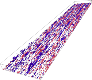
Figure 12 shows contours of scaled streamwise velocity fluctuations in the advection dominated region of the developing channel. Heated cases A-H $_2$O and A-C $Re_\tau^\star$ are shown in red in (a) and (b), while cooled cases D-H $_2$O and D-C $Re_\tau^\star$ are shown in blue in (c) and (d), respectively. The snapshots all taken at the same instant such that the inflow is the same. The $y$ location differs slightly for all the plots as it is kept such to have $y^{+}=15$ at $x/h = 0$ and then follows the streamline defined by $\tilde {u}$ and $\tilde {v}$. The comparison between A-H $_2$O and A-C $Re^{\star }_\tau$ shows clearly the diffusive effect of a larger viscosity, which tends to enlarge temperature structures. The same can be noticed by comparing D-C $Re^{\star }_\tau$ with D-H $_2$O. In addition, A-C $Re^{\star }_\tau$ shows a larger anisotropy compared with A-H $_2$O and conversely, the same can be noticed when comparing D-H $_2$O with D-C $Re^{\star }_\tau$. In the heated cases this detail is mostly visible in larger, high-momentum patches which, around $x/h \approx 6$, tend to decrease in intensity for case A-C $Re^{\star }_\tau$. Low-momentum streaks, on the other hand, decrease much more in intensity for case A-H $_2$O, showing a marked signature of viscous diffusion.

Figure 12. semilocal scaled velocity fluctuations;  $y^{+}_0 = 15$. Heated cases: (a) A-H $_2$O and (b) A-C $Re^{\star }_\tau$. Cooled cases: (c) D-H $_2$O and (d) D-C $Re^{\star }_\tau$.
We can conclude that, due to the local change in viscosity upon heating/cooling from the wall, we expect a larger impact of streamwise acceleration on A-C $Re^{\star }_\tau$ (and A-C $\mu$) over A-H $_2$O, deceleration on D-H $_2$O over D-C $Re^{\star }_\tau$. This impact is reflected in the parameter $\mathcal{C}_{ub}/\tau _w$ and can be studied by using semilocally scaled quantities. In the following sections we will investigate the effects of streamwise acceleration/deceleration on turbulent quantities, while contextualizing these effects in a variable property turbulence framework. Thanks to the specific boundary conditions chosen, leading to the slow streamwise evolution in region (iii), we study turbulence modulation in this region using semilocally scaled quantities as the cases are ‘self-similar’ in terms of semilocally scaled shear stress.
6. Turbulence modulation
To assess the direct impact of the advection  $\mathcal {C}_u$ on turbulent statistics, we analyse the normalized shear stress and turbulent stress, defined as
 \begin{equation} \Delta \mathcal{T} = \frac{\bar{\tau}_{xy}}{\tau_w} - \left( \frac{\bar{\tau}_{xy}}{\tau_{w}} \right)_{x/h=0}, \quad\Delta \mathcal{R} = \left( \frac{{\overline{\rho {u^{\prime \prime}} {v^{\prime \prime}}}}}{\tau_{w}} \right)_{x/h=0} - \frac{{\overline{\rho {u^{\prime \prime}} {v^{\prime \prime}}}}}{\tau_{w}} , \end{equation}
where  $\Delta \mathcal {T}$ and $\Delta \mathcal {R}$ represent the difference in viscous and turbulent shear stress between a streamwise location $x/h$ and the isothermal inlet. Figure 13 shows the profiles of $\Delta \mathcal {T}$ and $\Delta \mathcal {R}$ at $x/h=35$. The symbols in the right figure show profiles of difference in Reynolds stress assuming $\mathcal {C}_u$ is negligible,
 \begin{equation} \Delta \mathcal{R}^{eq} \equiv \Delta \mathcal{T} + \frac{\mathcal{C}_{ub}}{\tau_w} \frac{y}{h}. \end{equation}
It is possible to notice in figure 13(b) that for  $y^{\star } \lesssim 30$ $\Delta \mathcal {R} \approx \Delta \mathcal {R}^{eq}$, proving that the change in viscous shear stress is balanced entirely by the change in turbulent stress (as $\Delta \mathcal {T} \approx 0$ for $y^{\star } \gtrsim 50$) which is induced by a different pressure gradient ( $\mathcal {C}_{ub}/\tau _w$). In general, it is possible to state that, the shear stress increases (decreases) at the expense of the turbulent stress in accelerated (decelerated) flows, as already reported by Kline et al. (Reference Kline, Reynolds, Schraub and Runstadler1967) and Bushnell & McGinley (Reference Bushnell and McGinley1989). Following this observation, and what was stated in the previous section, we can study turbulence modulation following streamwise acceleration/deceleration devoid of any direct advection effects.

Figure 13. Difference in viscous ( $\Delta \mathcal {T}$) and turbulent ( $\Delta \mathcal {R}$) shear stress at $x/h = 35$. Symbols in panel (b) show profiles of turbulent shear stress assuming negligible advection (i.e. $\mathcal {C}_u = 0$) ( $\Delta \mathcal {R}^{eq}$).
Figure 14 shows the profiles of semilocally scaled turbulent stresses plotted using the  $y^{\star }$ coordinate. As for the velocity profile, the scaled streamwise fluctuations adjust very quickly within the buffer layer ( $y^{\star }<30$). On the other hand, the outer layer continues evolving to the change in bulk velocity. Three important observations can be made. (i) Cooled cases show features of a higher Reynolds number case (inflection point around $y^{\star } = 100$) while accelerated cases present a localized decrease of ${u}^{\prime \prime }$ in the outer layer, typical of a lower Reynolds number. This is expected given the evolution of Reynolds number in figure 3. (ii) The peak of ${u}^{\prime \prime }$ for case A-H $_2$O is significantly lower when compared with the other cases for which the collapse is somewhat acceptable. This can be attributed to the rapid decrease of Reynolds number to almost laminarizing values ( $Re_\tau \approx 150$). (iii) In the viscous sublayer ( $y^{\star } \leqslant 10$) the accelerated cases have lower ${u}^{\prime \prime }$ than the isothermal inlet, while D-H $_2$O has higher values. Moreover, spanwise and wall-normal fluctuation levels are much more affected by thermal development than streamwise fluctuation levels. Here ${v}^{\prime \prime }$ and ${w}^{\prime \prime }$ are greatly reduced for the heated cases and mildly increased for the cooled cases. Since this is consistent, despite the different constitutive laws for viscosity, it suggests that velocity fluctuations might scale with velocities typical of the outer layer instead of scaling with friction velocity.

Figure 14. Reynolds stress scaled with wall shear stress at  $x/h=15$ (a,c,e) and $x/h=35$ (b,d,f). (a,b) Streamwise component; (c,d) wall-normal component; (e,f) spanwise component.
As already stated in the previous section, the deviation of  $\bar {u}^{\star }$ suggests that the turbulence modulation is not only a product of local quantities but depends on non-local effects arising from the buffer layer and log-law region. Figure 15 shows profiles of streamwise and wall-normal velocity fluctuations normalized by a mixed velocity scale $u_m \equiv (u_\tau ^{\star } U_b)^{0.5}$, which accounts for outer-layer scaling. If normalized by the mixed velocity scale, streamwise fluctuation collapses perfectly in the viscous dominated region, with an overall improved agreement in the buffer layer. The same improvement is not immediately observed in the wall-normal component which still shows a large signature of streamwise acceleration/deceleration. On the other hand, the relative differences of the wall-normal velocity fluctuations, using this normalization, seem to be directly proportional to the deviations of streamwise fluctuations at larger $y^{\star }$. Indeed it is quite straightforward to relate the change of $v^{\prime \prime }$ between $10< y^{\star }<300$ to differences in the streamwise component between $30< y^{\star }<500$. This observation, in connection with the collapse of streamwise fluctuations in the viscous layer suggests that the effects of streamwise acceleration/deceleration are mostly felt by the wall-normal stress through the modulation of larger structures in the buffer and log-law region.

Figure 15. Velocity variances scaled with mixed velocity scale at  $x/h=15$ (a,c) and $x/h=35$ (b,d). (a,b) Streamwise velocity; (c,d) wall-normal velocity.
Figure 16 shows the averaged quadrants of Reynolds shear stress at  $x/h=35$. The impact of Q1 and Q3 is not discussed as these quadrants affect only marginally the Reynolds shear stress. As described by Patel et al. (Reference Patel, Boersma and Pecnik2016), variable properties mostly affect low-speed streaks (ejections) as these are strengthened with a decreased lift for a positive $Re_\tau ^{\star }$ gradient and vice versa for negative $Re_\tau ^{\star }$ gradient. Nonetheless, a general reduction in ejection intensity is visible for all the heated cases. The profiles of sweep strength (Q4) collapse quite consistently for the same $d_xU_b$ for $y^{\star }>10$ substantiating that variable properties impact more heavily the rising low-momentum structures, while sweeps are mostly affected by a change in bulk velocity. Nonetheless, the signature of acceleration/deceleration is largely visible in both ejection and sweep profiles, corresponding to a large decrease in the heated cases and a slight increase in the cooled cases. The larger impact of acceleration on sweep events might explain why the $u^{\prime \prime }$ scale better with mixed velocity scales, as sweeps are the most important mechanism of transfer of high-momentum outer-layer fluid towards the inner layer. Figure 17 shows the share of turbulent momentum transfer associated with positive and negative streamwise fluctuations at the centre and the end of the channel. It is clear that high-momentum streaks are more affected by streamwise acceleration/deceleration. In particular, in the buffer and log-law region ( $10< y^{\star }<100$), streamwise acceleration strongly decouples streamwise and wall-normal fluctuations, while streamwise deceleration has an opposite effect. This can be interpreted as a ‘straightening’ and ‘tilting’ of the high-speed streaks, that have a lower (higher) tendency of moving towards the walls. The same ‘straightening/tilting’ effect is felt on the low-momentum streaks but with a much lower intensity. This discrepancy in the response of low and high-momentum fluid can explain why the log-law constant for semilocally scaled transformed velocity $\bar {u}^{\star }$ increases for heated and decreases for cooled cases.

Figure 16. Normalized tangential Reynolds stress at  $x/h=35$ divided into quadrants: Q1 (outward motion), $u^{\prime \prime }>0, v^{\prime \prime }>0$; Q2 (ejection), $u^{\prime \prime }<0, v^{\prime \prime }>0$; Q3 (inward motion), $u^{\prime \prime }<0, v^{\prime \prime }<0$; Q4 (sweeps), $u^{\prime \prime }>0, v^{\prime \prime }<0$.

Figure 17. Normalized tangential Reynolds stress at  $x/h=35$ divided into contributions of positive and negative streamwise velocity fluctuation.
A more detailed analysis can be performed inspecting the anisotropy  $b_{ij}$, defined as
 \begin{equation} b_{ij} = \frac{\overline{\rho u_i^{\prime \prime} u_j^{\prime \prime}}}{2 k} - \frac{\delta_{ij}}{3} , \quad \text{where} \ k = 0.5(\overline{\rho {u^{\prime\prime}}^{2}}+\overline{\rho {v^{\prime\prime}}^{2}} +\overline{\rho {w^{\prime\prime}}^{2}} ) , \end{equation}
which is shown in figure 18. The cases with  $d_y{Re}_\tau ^{\star } =0$ represent test cases to benchmark the effect of acceleration, as, per the analysis of Patel et al. (Reference Patel, Boersma and Pecnik2016), only the gradient of the semilocal Reynolds number is of significance in a fully developed flow. For cases A-C $Re^{\star }_\tau$ and D-C $Re^{\star }_\tau$ we can notice an increase and decrease of anisotropy, respectively. This confirms a tendency of straightening and tilting of the quasi-streamwise vortices in the streamwise direction, which results in a modification of the wall-normal and spanwise fluctuation intensities. Contrarily to a fully developed flow, where the increase (or decrease) of $b_{11}$ is balanced entirely by the spanwise component $b_{33}$, acceleration and deceleration causes the increase/decrease of $b_{11}$ to be balanced equally in the spanwise and wall-normal direction. The same increase in anisotropy following a decrease in $v^{\prime }$ and $w^{\prime }$ was reported by Piomelli & Yuan (Reference Piomelli and Yuan2013) who also show the straightening of coherent eddies in FPG boundary layers. Once we understand the effects of thermal expansion and contraction on turbulence anisotropy, it is possible to isolate the effect of variable properties and $d_xU_b \neq 0$ in the other cases. In particular, $d_xU_b >0$ tends to increase anisotropy, opposing the effect of $d_y {Re}_\tau ^{\star } > 0$. Therefore, case A-H $_2$O, which is characterized by both these gradients, shows a localized decrease of anisotropy near the wall, where property gradients dominate, and an increase of anisotropy moving towards the buffer layer and the log-law region where acceleration effects prevail. Case D-H $_2$O which has opposite characteristics, shows the opposite behaviour. We can attribute the changes in $b_{22}$ almost entirely to $d_xU_b \neq 0$, as Patel et al. (Reference Patel, Boersma and Pecnik2016) have demonstrated that $b_{22}$ is not affected by property gradients in the wall-normal direction. This is substantiated by the fact that A-C $Re^{\star }_\tau$ (constant $Re_\tau ^{\star }$) has a larger deviation when compared with A-H $_2$O, and D-H $_2$O (larger deceleration impact) has a larger deviation when compared with D-C $Re^{\star }_\tau$. Nonetheless, it is possible to notice a slight impact of property variations on $b_{22}$ for case A-H $_2$O where, in the near-wall region, $b_{22}$ is (marginally) larger than the isothermal inlet.

Figure 18. Streamwise velocity normalized by inlet friction velocity along the inlet  $y^{+}$ at different streamwise locations. Lines as in figure 3. The black dashed–dotted line shows the isothermal inlet.
To further prove that the change in  $b_{22}$ is connected with acceleration, it is enough to show that it is abruptly modified in region (ii) and then experiences an extremely slow evolution in region (iii). Plots of streamwise evolution of $b_{11}$, $b_{22}$ and $b_{33}$ in the streamwise direction are shown for various cases in figure 19. As it is possible to notice, the streamwise component continues evolving for $x/h > 9$, and its evolution is counteracted by a change in the spanwise component. Contrarily, $b_{22}$ does not exhibit any particular change. This proves that the change in $\bar {u}^{\star }$ (which reflects the magnitude of the semilocal scaled viscous shear stress) is tightly connected to $b_{22}$. A higher (lower) anisotropy in the wall-normal direction necessarily leads to a lower (higher) $\bar {u}^{\star }$ (see figures 18 and 6) and, accordingly, collapsing semilocally transformed velocity is equivalent to having collapsed wall-normal anisotropy (see figures 19 and 7). A good example of this claim are cases A-C $Re^{\star }_\tau$ and A-C $\mu$, which have a collapsing $b_{22}$ value (despite being different from the isothermal inlet), and, correspondingly, the same profile of $\bar {u}^{\star }$. The connection between $b_{22}$ and $\bar {u}^{\star }$ is not limited to accelerated or decelerated cases, but applies to fully developed flows as well such as turbulent boundary layers where it is not possible to obtain a collapse of $\bar {u}^{\star }$. This claim ties together the observations on variable property flows made by Patel et al. (Reference Patel, Boersma and Pecnik2016) and Trettel & Larsson (Reference Trettel and Larsson2016) with the theory outlined by Townsend (Reference Townsend1961) and further developed by Bradshaw (Reference Bradshaw1967). The latter comments that turbulent motions at any point consist of two components, an ‘active’ component responsible for turbulent transfer and determined by stress distribution, and an ‘inactive’ component which does not transfer momentum or interact with averaged quantities. Townsend suggests that ‘the inactive motion is a meandering or swirling motion made up from attached eddies of large size’, and, therefore, it must be produced by the action of spanwise and streamwise fluctuating velocity. As Panton (Reference Panton2009) states, the wall-normal fluctuating component can be regarded entirely as active motion because of its primary role in momentum transfer. Patel's transformation, (3.1), therefore, demonstrates that ‘active’ turbulent motion scale with semilocal coordinate. Every other change noticed in anisotropy, vorticity fluctuation and mixing length can be attributed to ‘inactive turbulent motion’. Indeed, a modification of ‘active’ motion would necessarily reflect in the wall-normal anisotropy component and, by definition, on the scaled viscous shear stress. By following this reasoning it is possible to conclude that, contrarily to variable property effects, streamwise acceleration/deceleration affects active turbulent motion by acting directly on the wall-normal component.

Figure 19. Streamwise evolution of anisotropy profiles. (a–d) Streamwise anisotropy component  $b_{11}$. (e–h) Spanwise and wall-normal anisotropy component $b_{22}$ and $b_{33}$. Panels (a,e), (b,f), (c,g), (d,h) are case A-H $_2$O, case A-C $\mu$, case D-H $_2$O, case D-C $Re^{\star }_\tau$, respectively.
As  $b_{22}$ does not change significantly between $9< x/h<35$, (and consequently $\bar {u}^{\star }$), we can confirm that the structural change in ‘active’ turbulence occurs between $0< x/h<9$ (region (ii)), and in the rest of the channel the streamwise evolution occurs mainly due to property variation (and therefore, due to change in inactive turbulent component). Since active turbulence motions are in equilibrium, we can indeed consider the second half of the channel a ‘quasi-equilibrium’ layer where changes in mean variables dependent primarily on changes in local quantities (Panton Reference Panton2005). To better visualize the different turbulent states at play, figure 20 shows the barycentric map of the different cases at $x/h=35$ compared with the isothermal inlet. The three vertices of the equilateral triangle represent different anisotropic states. Now $x_{2C}$ is a pancake-like turbulent state, which is characterized by two main components, $x_{1C}$ is the one-component anisotropy limit, where turbulence exists in one direction only, while $x_{3C}$ is the isotropic limit. In a fully developed, constant property channel flow, the turbulence state tends to a pancake-like turbulence near the wall, shifts to cigar-shaped turbulence ( $x_{1C}$) in the streaky region, and eventually moves towards an isotropic state in the centre of the channel. While comparing the different cases, it is possible to notice that in the buffer region, the accelerating flows are closer to a one-component turbulence state when compared with the isothermal inlet. The opposite happens for case D-H $_2$O which is thermally contracted. It is important to notice that, the impact of acceleration (larger incidence of one-dimensional cigar-like structures) is damped in case A-H $_2$O when compared with A-C $Re^{\star }_\tau$ ( $Re_\tau ^{\star }$ gradient opposing $U_b$ gradient effects) but deceleration effects on turbulent structures are enhanced in the D-H $_2$O case despite variable property gradients counteracting pressure gradient effects. This confirms that viscosity plays a central role when opposing impulsive acceleration/deceleration, with an increase in viscosity always decreasing the effect of streamwise gradients, irrespective of the wall-normal $Re_\tau ^{\star }$ gradient.

Figure 20. Barycentric map of turbulent state along the wall-normal direction at  $x/h=35$.
Additional insight is provided by the normalized premultiplied spectra in the spanwise direction. Figure 21 shows contours of  $k_z E_{\rho u_i^{\prime \prime } u_i^{\prime \prime }}/\tau _w$ at $x/h = 35$ for the streamwise (a,d,g), wall-normal (b,e,h) and spanwise (c,f,i) components as a function of $\lambda _z^{\star } = \lambda _z {Re}_\tau ^{\star }/h$ and $y^{\star }$. As already noticed in Pei et al. (Reference Pei, Chen, Hussain and She2013) and confirmed by Patel et al. (Reference Patel, Boersma and Pecnik2016), the mean streak spacing in the near-wall region is smaller for $d_y{Re}_\tau ^{\star }>0$ and larger for $d_y{Re}_\tau ^{\star }<0$. This effect is visible as the tilting of the streamwise energy spectra near the wall (towards lower $\lambda ^{\star }_z$ in the first case and larger $\lambda _z^{\star }$ in the second). The absence of a near wall-shift for case A-C $Re^{\star }_\tau$ substantiates that the latter is caused solely by the $Re_\tau ^{\star }$ wall-normal gradient. The spanwise component also presents the same tilt, which is, on the other hand, completely absent in the wall-normal component. This is consistent with the claim that turbulent motions below $y^{\star }=10$ are mostly inactive and don't carry significant shear stress. Looking at buffer layer effects, which, in a variable property fully developed channel flow scale properly with semilocal coordinates ( $y^{\star }$ and $\lambda _z^{\star }$), it is possible to pinpoint the streamwise acceleration/deceleration effects. The occurrence of larger streaks is lower in case A-C $Re^{\star }_\tau$ and A-H $_2$O and higher in the case D-H $_2$O. Contrarily to the effect of variable properties, this reduction (increase) in energy share at larger wavenumbers is consistent throughout all the components. Taking A-C $Re^{\star }_\tau$ as a benchmark, spectral effects of streamwise acceleration (deceleration) can then be summarized as a lower (larger) spectral energy transfer rate and a general reduction (increase) of streak spacing. This analysis is compatible with the anisotropy effects discussed with figures 18 and 20 and is a proof of the elastic streamwise stretching (contracting) of the streaks following a streamwise acceleration (deceleration). The fact that the reduction (increase) in large wavenumber energy density is consistent throughout all components clearly connects the effect of streamwise acceleration/deceleration to pressure fluctuations, which are indeed more sensitive to the changes in larger overhead structures (Townsend Reference Townsend1976; Kim Reference Kim1988; Katul et al. Reference Katul, Albertson, Hsieh, Conklin, Signmon, Parlange and Knoerr1996; Gerolymos, Senechal & Vallet Reference Gerolymos, Senechal and Vallet2013). The results shown in figure 21 are in accordance with the study from Bobke et al. (Reference Bobke, Vinuesa, Örlü and Schlatter2017), which reports an increase in energy contained in the larger turbulent structures in an adverse pressure gradient boundary layer. They also notice that the near-wall peak is insensitive to the adverse pressure gradient, as it is shown for the constant $Re_{\tau }^{\star }$ case in figure 21.

Figure 21. One-dimensional spanwise premultiplied spectra for  $u$ (a,d,g), $v$ (b,e,h) and $w$ (c,f,i). Filled contour is at $x/h = 0.02$ while lines are at $x/h=35$. Panels (a,d,g), (b,e,h), (c,f,i), are streamwise energy spectra $k_z E_{\rho u^{\prime \prime } u^{\prime \prime }}/\tau _w$, wall-normal energy spectra $k_z E_{\rho v^{\prime \prime } v^{\prime \prime }}/\tau _w$, spanwise energy spectra $k_z E_{\rho w^{\prime \prime } w^{\prime \prime }}/\tau _w$, respectively. Panels (a,b,c), (d,e,f), (g,h,i), are case A-C $Re^{\star }_\tau$, case A-H $_2$O and case D-H $_2$O respectively.
7. Intercomponent energy transfer
The budget equation for turbulent stresses in a variable property turbulent flow reads
 \begin{align} \frac{\partial
{\overline{\rho u^{\prime \prime}_i u^{\prime
\prime}_j}}}{\partial t} + \frac{\partial \tilde{u}_k
{\overline{\rho u^{\prime \prime}_i u^{\prime
\prime}_j}}}{\partial x_k} &= \underbrace{- \left(
\overline{\rho u^{\prime \prime}_i u^{\prime
\prime}_k}\frac{\partial \tilde{u}_j}{\partial x_k} +
\overline{\rho u^{\prime \prime}_j u^{\prime
\prime}_k{}}\frac{\partial \tilde{u}_i}{\partial x_k}
\right)}_{\mathcal{P}_{ij}}+ \nonumber\\ &\quad
+\frac{\partial}{\partial x_k} \left(
-\overline{\rho u^{\prime \prime}_i u^{\prime \prime}_j
u^{\prime \prime}_k} + \overline{u^{\prime \prime}_i
\tau_{jk}^{\prime}} + \overline{u^{\prime \prime}_j
\tau_{ik}^{\prime}}\right)+ \nonumber\\ &\quad
\underbrace{- \overline{ \left( u^{\prime
\prime}_j\frac{\partial p^{\prime}}{\partial x_i} +
u^{\prime \prime}_i\frac{\partial p^{\prime}}{\partial x_j}
\right)}}_{\varPi_{ij}} -
\underbrace{\overline{\tau_{jk}^{\prime} \frac{\partial
u^{\prime \prime}_i}{\partial x_k} + \tau_{ik}^{\prime}
\frac{\partial u^{\prime \prime}_j}{\partial x_k}
}}_{\varepsilon_{ij}} + \nonumber\\ &\quad +
\overline{u^{\prime \prime}_i} \left( \frac{\partial
\bar{\tau}_{jk}}{\partial x_k} - \frac{\partial
\bar{p}}{\partial x_j} \right) +\overline{u^{\prime
\prime}_j}\left( \frac{\partial \bar{\tau}_{ik}}{\partial
x_k} - \frac{\partial \bar{p}}{\partial x_i} \right).
\end{align}
\begin{align} \frac{\partial
{\overline{\rho u^{\prime \prime}_i u^{\prime
\prime}_j}}}{\partial t} + \frac{\partial \tilde{u}_k
{\overline{\rho u^{\prime \prime}_i u^{\prime
\prime}_j}}}{\partial x_k} &= \underbrace{- \left(
\overline{\rho u^{\prime \prime}_i u^{\prime
\prime}_k}\frac{\partial \tilde{u}_j}{\partial x_k} +
\overline{\rho u^{\prime \prime}_j u^{\prime
\prime}_k{}}\frac{\partial \tilde{u}_i}{\partial x_k}
\right)}_{\mathcal{P}_{ij}}+ \nonumber\\ &\quad
+\frac{\partial}{\partial x_k} \left(
-\overline{\rho u^{\prime \prime}_i u^{\prime \prime}_j
u^{\prime \prime}_k} + \overline{u^{\prime \prime}_i
\tau_{jk}^{\prime}} + \overline{u^{\prime \prime}_j
\tau_{ik}^{\prime}}\right)+ \nonumber\\ &\quad
\underbrace{- \overline{ \left( u^{\prime
\prime}_j\frac{\partial p^{\prime}}{\partial x_i} +
u^{\prime \prime}_i\frac{\partial p^{\prime}}{\partial x_j}
\right)}}_{\varPi_{ij}} -
\underbrace{\overline{\tau_{jk}^{\prime} \frac{\partial
u^{\prime \prime}_i}{\partial x_k} + \tau_{ik}^{\prime}
\frac{\partial u^{\prime \prime}_j}{\partial x_k}
}}_{\varepsilon_{ij}} + \nonumber\\ &\quad +
\overline{u^{\prime \prime}_i} \left( \frac{\partial
\bar{\tau}_{jk}}{\partial x_k} - \frac{\partial
\bar{p}}{\partial x_j} \right) +\overline{u^{\prime
\prime}_j}\left( \frac{\partial \bar{\tau}_{ik}}{\partial
x_k} - \frac{\partial \bar{p}}{\partial x_i} \right).
\end{align}
As already demonstrated in the previous section, direct advection effects on turbulence modulation can be neglected in the ‘quasi-homogeneous’ region. Additionally, terms containing  $\overline {u^{\prime \prime }}$ are small as they play a role only in high Mach number supersonic flows. The interplay of intercomponent energy exchange which sustains a modified flow anisotropy in accelerated/decelerated flows must, therefore, be a result of the changes in the balance of production $\mathcal {P}_{ij}$, dissipation $\varepsilon _{ij}$ and velocity-pressure-gradient correlation $\varPi _{ij}$. Note, unlike as is commonly done, we did not decompose $\varPi _{ij}$ into pressure transport and pressure-strain correlation.
In a turbulent flow, the turbulent kinetic energy is produced by mean shear. Streamwise velocity fluctuations are directly dissipated through viscosity ( $\varepsilon _{11}$) and redistributed to the other components through the correlation between the velocity and the pressure-gradient fluctuations. Figure 22 shows production and dissipation terms for the streamwise velocity component at the end of the channel. The peak of turbulent production aligns for all cases at $y^{\star } \approx 12$, reinforcing the observation that semilocal scales are the correct tool to study turbulence modulation in variable property flows even when subjected to acceleration and deceleration. Nonetheless, turbulent production increases consistently for cooled cases and decreases for heated ones. This is expected as the mean shear in a flow subjected to acceleration increases in the viscous region, with little to no effect on the turbulent production, while it decreases farther away from the wall, decreasing substantially turbulent production (Kline et al. Reference Kline, Reynolds, Schraub and Runstadler1967; Bushnell & McGinley Reference Bushnell and McGinley1989; Nemati Reference Nemati2016). The opposite happens for decelerated flows. On the other hand, as seen in the central figure and confirmed by the $\mathcal {P}_{11}/\varepsilon _{11}$ ratio (figure 22c), viscous dissipation does not show the same level of susceptibility to acceleration/deceleration. As a consequence, there is a (slight) excess of turbulent energy for the decelerated cases and, vice versa, a shortage in the accelerated cases. This observation is in accordance with the claim that streamwise acceleration/deceleration modulate large, energy containing structures and do not affect as strongly the smaller dissipative structures in the buffer layer. In accordance with the results observed by Tuerke & Jimenez (Reference Tuerke and Jimenez2013), following a change in mean shear the production of turbulent kinetic energy responds much more quickly than viscous dissipation. This is intuitive since the mean shear directly acts on energy containing eddies, whereas viscous dissipation occurs at smaller dissipative scales. Tuerke & Jimenez (Reference Tuerke and Jimenez2013) showed that the change in production is balanced by turbulent transport, which redistributes energy to locations at which viscous dissipation is more responsive. In our case, the production increase/decrease is balanced by $\varPi$ (shown, normalized by $\varepsilon _{11}$ in figure 23) which is known to be affected mostly through non-local interactions arising from the large energy-containing scales in the buffer layer (Katul et al. Reference Katul, Albertson, Hsieh, Conklin, Signmon, Parlange and Knoerr1996).

Figure 22. Production and dissipation terms for the streamwise component at  $x/h=35$.

Figure 23. Pressure-strain correlation for all three velocity components, normalized by streamwise dissipation.
As seen by figure 21, this occurs because of the preferential decrease (increase) in production of the large energy containing structures at  $y^{\star }>20$. Despite all the profiles of $\varPi _{11}$ showing a decrease in intensity for the heated cases, the impact of variable properties is noticed for the streamwise and spanwise pressure terms, where a local increase in magnitude near the wall is visible for case A-H $_2$O. Since A-H $_2$O has an increasing $Re_\tau ^{\star }$ in the wall-normal direction, the streamwise vortices tend to destabilize (as shown in Rinaldi et al. (Reference Rinaldi, Patel, Schlatter and Pecnik2017)), and thus counteract the effect of acceleration. This is particularly visible for $y^{\star } < 15$, where $\varPi _{11}/\varepsilon _{11}$ is higher than for the reference inlet profile. The increase in magnitude of $\varPi _{ij}/\varepsilon _{11}$ is minimal for the wall-normal component confirming that the turbulent energy flows from the streamwise to the spanwise component in this region. This reinforces the claim that wall-normal anisotropy is not significantly affected by local quantities (in contrast to the other two components). Contrarily to the viscous dissipation of $u^{\prime \prime }$, the dissipation of the other two components, shown in figure 24, balances the pressure term. For this reason, the lower/higher pressure terms has a direct effect on turbulence anisotropy.

Figure 24. Viscous dissipation in wall-normal and spanwise direction, normalized by viscous dissipation in the streamwise direction.
Figure 25 shows  $\varPi _{ij}$ normalized by $\tau _w^{2}/\bar {\mu }$ (Foysi et al. Reference Foysi, Sarkar and Friedrich2004). Foysi et al. (Reference Foysi, Sarkar and Friedrich2004) showed that for compressible channel flows with $d_y \bar {\rho }<0$, the intercomponent energy transfer reduces significantly due to the reduction of pressure fluctuations. Specifically, pressure gradient is a force at a distance and incorporates ‘non-local’ density effects integrated over the whole turbulent eddy. In a case in which density decreases with the distance from the wall, the ‘effective’ averaged density experienced from the pressure gradient would be lower than for an incompressible flow, leading to lower values of $\varPi _{ij}$. We expect, therefore, that the opposite occurs for a case with $d_y \bar {\rho }>0$. Following the analysis detailed above, and neglecting acceleration, one would expect a larger $\varPi$ for the heated cases and vice versa for the cooled cases (the density increases from the walls in the former and decreases in the latter). Figures 25 and 23 negate this premise as the expected behaviour is observed only marginally at $y^{\star }<10$. Nevertheless, as observed by Foysi et al. (Reference Foysi, Sarkar and Friedrich2004), the fact that the $\varPi$ terms do not conserve the location of the peak when normalized by $\tau _w/\bar {\mu }$ is proof that the velocity-pressure-gradient correlation does not scale with inner-layer variables (it is connected to the changes of outer-layer motions). This might be the reason for the failure of semilocal scaling to collapse viscous stresses in developing flows where pressure responds to changes in mean shear. Indeed, the marginal effect of a wall-normal $Re^{\star }_\tau$ gradient on $\varPi _{22}$ (compared with $\varPi _{11}$ and $\varPi _{33}$) explains why active motions that carry momentum towards the walls (and away from the wall) scale with local quantities in fully developed turbulence and, as a consequence, why viscous stresses collapse using semilocally scaled coordinates.

Figure 25. Pressure-strain correlation for all three velocity components, normalized by  $\tau _w^{2}/\bar {\mu }$.
Figure 26 shows the anisotropy component of the dissipation tensor, defined as
 \begin{equation} d_{ij} = \frac{\varepsilon_{ij}}{\varepsilon_{11}+\varepsilon_{22}+\varepsilon_{33}} - \frac{\delta_{ij}}{3}. \end{equation}
In particular, the heated flows are characterized by a larger share of turbulent kinetic energy dissipation in the streamwise direction and lower in the other two directions. This is consistent with the observation that throughout the developing channel the changes in  $\mathcal {P}_{11}$ are balanced by $\varPi _{11}$. As such, the streamwise viscous dissipation is not severely affected, but its spanwise and wall-normal counterparts, which directly balance pressure-strain production, are reduced largely. This leads to a larger reduction in wall-normal and spanwise components which causes a larger (lower) anisotropy, justifying the schematic seen in figure 20. In addition, since this mechanism is related to non-local pressure fluctuations adapting to the mean shear stress imposed by the change in bulk velocity, it is immediately understandable why the collapse of velocity profiles following a semilocal scaling approach (viscous shear stress transformation) is not possible. In the near-wall region, the anisotropy of the dissipation carries the signature of variable properties effects, showing a direct relation with the profiles of $b_{ij}$ (figure 18). As $y^{\star } \rightarrow 0$, the energy containing scales overlap with the dissipative scales, therefore closely relating $d_{ij}$ to $b_{ij}$ (Antonia, Djenidi & Spalart Reference Antonia, Djenidi and Spalart1994). This also confirms that, contrarily to streamwise acceleration/deceleration, which originates differences on the large velocity structures in the outer layer, variable properties locally affect the dissipation near the wall. If this is the case, it is clear why active turbulent motions collapse perfectly in a fully developed variable property channel.

Figure 26. Anisotropy of the dissipation tensor at  $x/h=35$.
Figure 27 presents an additional proof of the fact that pressure effects due to streamwise acceleration are felt more by the high-speed streaks rushing towards the wall. On the left- and right-hand side, the conditionally averaged pressure-strain correlation in the streamwise direction for low- and high-speed streaks is shown, respectively, normalized by the total viscous dissipation in streamwise direction (to keep a consistency with figure 23). Comparing figure 27 with the previously shown streamwise pressure-strain correlation (figure 23) it is clear that the major deviations occur in the terms that contain  $u^{\prime \prime }>0$, i.e. the high-speed streaks. The ratio of $\varPi _{11}$ to $\varepsilon _{11}$ remains more similar to the inlet condition for $u^{\prime \prime }<0$, and, keeping in mind that we before claimed that viscous dissipation is locally modulated by variable properties, this is another proof that low-speed streaks originating near the walls and moving towards the centre of the channel are more prone to be modulated by local quantities. On the other hand, high-speed streaks show consistent behaviour for accelerated and decelerated cases in terms of $\varPi _{11}/\varepsilon _{11}$ beyond $y^{\star }=20$. This implies that high speed streaks are less sensitive to $Re_{\tau }^{\star }$ gradients (as they originate farther from the wall), but more sensitive to changes in the mean shear which are caused by a streamwise change in bulk velocity.

Figure 27. Pressure strain in the streamwise direction normalized by viscous dissipation of the streamwise velocity component at  $x/h=35$.
8. Conclusions
We have shown turbulence modulation for a variety of streamwise accelerating and decelerating flows characterized by different property variations. We first showed that, if the flow is subjected to an impulsive acceleration, the change in turbulence structure occurs rapidly and then follows a slow evolution in which the turbulence state can be considered ‘quasi-homogeneous’. This occurs because of two different reasons. Firstly, we showed that the wall-normal property gradients (if sufficiently close to the wall), characterized by the semilocal Reynolds number  $Re_\tau ^{\star }$, modify only the ‘inactive’ turbulent motions, which carry energy but no tangential stress (Townsend Reference Townsend1976), while the active turbulent motions scale with local quantities. This is why, in fully developed turbulent channel flows, the mean quantities of interest collapse to universal profiles in a semilocal framework (as noticed by Patel et al. (Reference Patel, Peeters, Boersma and Pecnik2015) and Trettel & Larsson (Reference Trettel and Larsson2016)). Secondly, streamwise acceleration/deceleration directly modify active turbulent motions only in the immediate aftermath of the impulsive acceleration. As a consequence, all relevant averaged quantities are self-similar at a location sufficiently downstream if scaled through local values.
Next, we distinguished the effect of streamwise acceleration/deceleration from the effects of wall-normal property gradients and showed that the two effects can be superimposed once the strength of the bulk advection is known. In particular, while variable properties affect mostly the strength and the consequent lift-up of near-wall low-momentum streaks, streamwise acceleration/deceleration mostly acts on the larger structures in the buffer layer. This causes a reduction/increase in the sweeping events of high-momentum fluid towards the wall. Since the impact of streamwise acceleration/deceleration is more prominent at larger scales of motion (and affects mostly sweeping events), it percolates towards the wall through pressure strain effects. In particular, pressure fluctuations connected to the high-momentum fluid impinging on the wall decrease in intensity for accelerating flows. A consequence of the reduced pressure fluctuations is the stabilization of the turbulent structures. This decreases the velocity-pressure-gradient correlation reducing the energy transferred to the wall-normal and spanwise fluctuation components. Therefore, contrarily to a pure property gradient effect, which acts locally on the dissipative scales, streamwise acceleration/deceleration produce a non-local effect causing a higher anisotropy in accelerated and lower anisotropy in decelerated cases. The extent of this change is quantified by the normalized bulk advection term  $\mathcal {C}_{ub}/\tau _w$ which is enhanced by a decrease in viscosity, and reflected in the semilocally scaled wall-normal anisotropy component.
To summarize, turbulence modulation by the wall-normal gradient of  $Re_\tau ^{\star }$ (variable property effects) and the streamwise gradient of $U_b$ (acceleration/deceleration effect), follow an opposite mechanism in terms of intercomponent energy transfer. The first can be summed up as a ‘bottom-up’ mechanism, whereas local properties affect viscous dissipation which in turn modulates momentum transfer. As a consequence, the most affected bursting events are low-speed streaks which travel upwards towards the centre of the channel. This mechanism, as it originates from viscous dissipation, depends on local variables and (as long as the largest property gradients are close to the walls) is fully described by semilocal scaling. Streamwise acceleration/deceleration, on the other hand, acts mostly on the larger energy-containing structures in the buffer layer by modifying the mean shear. The response from the turbulent flow is felt through the velocity-pressure-gradient correlation, which leads to a different redistribution of energy through the velocity components. The changes in anisotropy manifest in an accelerated flow with longer, more stable structures through a process of ‘stretching’ while, vice versa, shorter compressed turbulent structures are found in the presence of deceleration. Contrarily to property gradients, acceleration/deceleration impacts more heavily high-momentum streaks which originate in the buffer layer. As the modification occurs because of the larger outer-layer scales’ influence on pressure, the ‘non-locality’ of this mechanism is not included in the semilocal scaling representation, despite the state of ‘quasi-homogeneity’ in the streamwise direction.
Acknowledgements
The authors report no conflict of interest.


 Open access