


1. Introduction
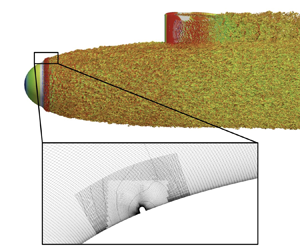
Tripping devices are an extensively used method of fixing the turbulent transition location of boundary layers in down-scaled model experiments to suppress the influence of experimental tunnel conditions on natural transition and produce Reynolds number similarity to the full-scale model. The enforcement of a fixed transition location also simplifies the comparison of experiments with numerical simulations. As described by Preston (Reference Preston1958), the role of the trip is to (i) artificially increase the boundary layer momentum thickness to the minimum value required for a turbulent boundary layer (TBL) and (ii) provide a disturbance to immediately transition the flow from a laminar to a turbulent state. Figure 1 shows a diagram of the development of a laminar boundary layer encountering a trip wire and the subsequent evolution of the TBL. The TBL downstream of the trip should ideally have no memory of the tripping configuration to satisfy similarity and to permit comparison between different experiments and computations. While tripping is essential in a variety of contexts, there are potential hazards associated with tripping that have come to light over the years, including memory of tripping effects as the boundary layer develops.

Figure 1. Diagram of the evolution of a boundary layer with a trip wire.
With the advent of increased computational power and advanced numerical methods, high-fidelity turbulent simulations have increasingly been employed in both basic research and engineering contexts. While in many cases periodic boundary conditions or re-scaling methods implicitly avoid the dependence on the tripping device (at the cost of introducing other challenges), external aerodynamic and hydrodynamic flows most often have no such luxury. Given the restriction of high-fidelity large-eddy simulations (LES) and direct numerical simulations (DNS) to low to moderate Reynolds numbers where tripping effects may persist, it is perhaps surprising that few LES and DNS have resolved the experimental trip geometry, besides those studies focused on near-field trip-induced instabilities (table 1 gives a sample of past DNS/LES with the corresponding experimental and numerical tripping methods). This may be due to the traditional assumption that the memory of the trip is lost, the lack of specifics of the trip geometry in experimental work or the practical difficulty of resolving the trip in simulations. As a result, most simulations use an artificial tripping strategy to induce transition, such as suction/blowing, immersed boundary forcing or a step in the numerical grid.
Table 1. Sample of past LES and DNS of external flows and the tripping method used in the simulations, where ZPGTBL refers to zero-pressure-gradient TBL. Studies that are specifically focused on capturing trip-induced instabilities are neglected (e.g. Muppidi & Mahesh Reference Muppidi and Mahesh2012; Subbareddy, Bartkowicz & Candler Reference Subbareddy, Bartkowicz and Candler2014; Kurz & Kloker Reference Kurz and Kloker2016; Shrestha & Candler Reference Shrestha and Candler2019; Ma & Mahesh Reference Ma and Mahesh2022).

1.1. Tripping of flat-plate zero-pressure-gradient boundary layers
Despite this lack of resolved trip simulations, the proper tripping of flat-plate zero-pressure-gradient TBLs (ZPGTBLs) has been considered. Early studies focused on establishing criteria for trip sizing, which were often formulated based on a minimum trip Reynolds number,  $Re_d = U_d d / \nu$ (Fage, Preston & Relf Reference Fage, Preston and Relf1941; Gibbings Reference Gibbings1959). In this definition, $d$ is the trip wire diameter, $\nu$ is the kinematic viscosity and $U_d$ is the velocity in the incoming boundary layer at a distance $d$ from the wall, as labelled in figure 1. While a number of criteria for $Re_d$ have been proposed, it is notable that these numbers may be influenced by experimental free-stream turbulence, surface roughness and vibrations (Jones et al. Reference Jones, Erm, Valiyff and Henbest2013) and do not account for the effects of pressure gradients or curvature. Preston (Reference Preston1958) suggested that trips should artificially raise the momentum thickness Reynolds number to a proposed lower limit of $Re_\theta = U_\infty \theta / \nu = 320$ for TBLs (where $U_\infty$ is the free-stream velocity and $\theta$ is the boundary layer momentum thickness). In terms of the perturbation introduced by the trip, it may act in two capacities: (i) the production of vigorous temporally growing disturbances to induce immediate transition through an absolute instability, or (ii) a slower convective instability growth acting through amplification of spatially growing upstream disturbances. While the second form does lead to transition of the boundary layer further upstream than without a trip wire, the transition location is dependent on the level of background noise. Therefore, the overarching purpose of $Re_d$ criteria is to select a trip size that will induce an absolute (global) instability.
The choice of the trip geometry itself has also been the subject of experimental scrutiny. In their pioneering study of trip devices, Klebanoff & Diehl (Reference Klebanoff and Diehl1951) found that it was possible to satisfactorily artificially thicken a boundary layer, but the distance required for tripping effects to disappear varied with the choice of tripping device. Later, Preston (Reference Preston1958) identified the trip wire as the most suitable trip geometry due to its simplicity compared with air jets and wall-normal strips and minimal effect on the outer velocity distribution compared with slotted strips and sandpaper. A result of these studies has been concept of ‘over-tripping’ (over-stimulation) of the flow. While this term has no formal definition, it has been associated with violating the proposed  $Re_d$ criteria by grossly exceeding the minimum trip size to promote immediate transition of the boundary layer. However, even when adhering to the $Re_d$ criteria, over-tripping is difficult to avoid at low Reynolds numbers, where the selection of a trip height at the required $Re_d$ to produce an absolute instability may inevitably lead to the trip size exceeding the boundary layer thickness. Often, this is avoided by placing trips after the Tollmien–Schlichting convective instability point of the Blasius boundary layer ( $Re_\theta = 200$ or $Re_{\delta ^*} = U_\infty \delta ^* / \nu = 520$, where $\delta ^*$ is the boundary layer displacement thickness), although this is not strictly necessary and infeasible in some contexts. While over-tripping does not necessarily lead to an excess in skin friction, it typically results in a TBL that ‘feels’ a persisting effect of the tripping device far downstream, and does not conform to what is considered a ‘well-behaved’ (canonical) TBL (Jones et al. Reference Jones, Erm, Valiyff and Henbest2013). Specific characteristics of over-tripping are an excessive momentum thickness jump across the trip and the introduction of low frequencies in the outer layer (Erm & Joubert Reference Erm and Joubert1991; Marusic et al. Reference Marusic, Chauhan, Kulandaivelu and Hutchins2015).
Even in scenarios that avoid over-tripping by using proper boundary layer stimulation, there have been questions of the persisting effect of upstream conditions on TBLs. Castillo & Johansson (Reference Castillo and Johansson2002) found that boundary layer defect profiles across a range of  $Re_\theta$ collapsed against $U_\infty$ only when the upstream conditions (free-stream velocity and tripping) were held constant, meaning that only the measurement location was varied to span the $Re_\theta$ range. This runs counter to the traditional idea that the boundary layer should be independent of these choices of upstream conditions.
These history effects have been found to be most prominent at low  $Re_\theta$, as confirmed by both experimental and numerical studies. Erm & Joubert (Reference Erm and Joubert1991) performed a pioneering study of the recovery of low- $Re_\theta$ ( $715 \le Re_\theta \le 2810$) TBLs from several tripping geometries (circular wire, cylindrical pins and grit) at different free-stream velocities. The effect of the free-stream velocity was to under- or over-stimulate the flow if above or below the velocity of the design condition, which suggests that trips must be sized for each free-stream velocity to properly stimulate the flow. However, this is rarely done in practice, as researchers typically seek only a match of the local Reynolds number when comparing TBLs, which implicitly ignores the effect of the tripping device on the boundary layer development. In over-tripped cases, Reynolds stress profiles and spectra only began to collapse at $Re_\theta \approx 2175$, while proper stimulation led to a collapse at $Re_\theta \approx 1020$. An experimental study of different trips at fixed unit Reynolds number ( $U_\infty /\nu$) by Marusic et al. (Reference Marusic, Chauhan, Kulandaivelu and Hutchins2015) revealed a much longer memory of the trip that lasted until $Re_\theta \approx 27\,000$, corresponding to $Re_x = x U_\infty /\nu \approx 1.7 \times 10^7$. They found that the turbulence intensity for over-tripped cases did not collapse for either matched $Re_x$ or matched local Reynolds number ( $Re_\theta$ or $Re_\tau$), and both Marusic et al. (Reference Marusic, Chauhan, Kulandaivelu and Hutchins2015) and Sanmiguel Vila et al. (Reference Sanmiguel Vila, Vinuesa, Discetti, Ianiro, Schlatter and Örlü2017) observed large-scale turbulent structures in the outer layer in over-tripped cases. These results highlight the danger of comparing with experiments at matched $Re_x$, $Re_\tau$ or $Re_\theta$ without consideration of upstream conditions.
A complimentary numerical study using DNS was performed by Schlatter & Örlü (Reference Schlatter and Örlü2012), who studied the differences between flat-plate ZPGTBLs developing from different numerical tripping conditions. They found that the stark differences in the skin friction coefficient and shape factor between ZPGTBL DNS datasets (Schlatter & Örlü Reference Schlatter and Örlü2010) were due to the way in which transition was initiated. They concluded that integral, mean and higher-order statistics agree well between simulations for  $Re_\theta > 2000$ as long as transition was initiated below the edge of the laminar boundary layer for $Re_\theta < 300$ while avoiding under- or over-stimulation, as echoed by Silvestri et al. (Reference Silvestri, Ghanadi, Arjomandi, Cazzolato and Zander2018). Notably, however, their study was limited to numerical tripping models (different frequencies and amplitudes of random wall-normal volume forcing), and the trip device itself was not resolved. Kozul et al. (Reference Kozul, Chung and Monty2016) performed DNS of a temporally developing TBL with a hyperbolic tangent initial condition designed to replicate the recirculation region behind a trip wire. They concluded that the $Re_\theta$ required for statistical collapse increased linearly with the trip Reynolds number since memory effects were lost as $\theta /d$ of the TBL reached unity, although the differences between temporally and spatially developing TBLs may limit the applicability of this assessment.
1.2. Tripping of boundary layers on external flow models
These flat-plate ZPGTBL studies raise important questions about ZPGTBLs that are perceived as canonical in both experimental and numerical contexts (Hutchins Reference Hutchins2012), but do not begin to address the more complex tripping effects on more complex geometries. Additionally, these studies have been limited to numerical tripping approximations in simulations (Schlatter & Örlü Reference Schlatter and Örlü2012; Kozul et al. Reference Kozul, Chung and Monty2016) and limited sets of measurements in experiments (Erm & Joubert Reference Erm and Joubert1991; Marusic et al. Reference Marusic, Chauhan, Kulandaivelu and Hutchins2015; Sanmiguel Vila et al. Reference Sanmiguel Vila, Vinuesa, Discetti, Ianiro, Schlatter and Örlü2017).
In addition, for external flow around a model, one can argue that it is not enough to solely trip the model to produce a canonical TBL at matched local Reynolds numbers ( $Re_\theta$ and $Re_\tau$), since the geometry of the model imposes that a suitable TBL must also be achieved at matched $Re_x$. While one may have the luxury of providing a post-trip ‘development length’ for flat-plate boundary layers, this is often not possible in the context of flow around a model. Additionally, the TBL development is more complex for these external flows due to the progression of the boundary layer through pressure gradients, streamline curvature and possibly junction flows (figure 1). Despite these issues and the documented inconsistencies for flat plate TBLs, relatively little attention has been paid to tripping effects on more complex geometries. Erm, Jones & Henbest (Reference Erm, Jones and Henbest2012) and Jones et al. (Reference Jones, Erm, Valiyff and Henbest2013) studied the effect of different tripping geometries at a fixed position on the Joubert notional axisymmetric hull in the process of selecting a suitable trip. dos Santos, Venner & de Santana (Reference dos Santos, Venner and de Santana2022) performed measurements with several trip geometries on a NACA0012 airfoil at zero angle of attack. They found that while the type of tripping device influenced the boundary layer development, it did not affect the boundary layer characteristics at the trailing edge. However, the trip height significantly affected the boundary layer thickness and shape factor at the trailing edge and introduced low frequencies in the turbulent velocity spectra and wall-pressure fluctuations (dos Santos et al. Reference dos Santos, Even, Botero, Venner and de Santana2021). For an appended model, such as an airplane or submarine, the presence of appendages results in junction flows that may be influenced by tripping effects through their impact on the incoming boundary layer thickness (Fleming, Simpson & Devenport Reference Fleming, Simpson and Devenport1991) and fluctuations in the outer layer (Devenport & Simpson Reference Devenport and Simpson1990).
1.3. The present study
With these details in consideration, the present study seeks to investigate the effect of the tripping method on the high-fidelity simulation of flow around a model-scale geometry through trip-resolved LES. In particular, this work adds to the existing literature by resolving the experimental trip wire in the computations, considering tripping in the presence of pressure gradients and streamline curvature, and comparing the resolved trip computations with a much simpler artificial numerical trip. The geometry under consideration is the DARPA SUBOFF, a well-studied axisymmetric streamlined hull with a sail and four stern appendages in a cross shape (Groves et al. Reference Groves, Huang and Chang1989), as depicted in figure 2. The axisymmetric (bare hull) and fully appended configurations of the DARPA SUBOFF have been studied through a series of experiments (Huang et al. Reference Huang, Liu, Groves, Forlini, Blanton and Gowing1992; Jiménez, Hultmark & Smits Reference Jiménez, Hultmark and Smits2010b; Jiménez, Reynolds & Smits Reference Jiménez, Reynolds and Smits2010c) and computations using Reynolds-averaged Navier–Stokes simulations (Toxopeus Reference Toxopeus2008; Sezen et al. Reference Sezen, Dogrul, Delen and Bal2018), detached-eddy simulations (Bhushan, Alam & Walters Reference Bhushan, Alam and Walters2013; Chase & Carrica Reference Chase and Carrica2013) and LES (Posa & Balaras Reference Posa and Balaras2016, Reference Posa and Balaras2018, Reference Posa and Balaras2020; Kumar & Mahesh Reference Kumar and Mahesh2018b; Morse & Mahesh Reference Morse and Mahesh2021). Note that none of these past simulations have numerically resolved the trip geometry, and have instead used different numerical strategies to promote transition.

Figure 2. Geometry of (a) bare hull (AFF1) and (b) fully appended (AFF8) configurations of the DARPA SUBOFF (Groves, Huang & Chang Reference Groves, Huang and Chang1989).
We consider two flow configurations: (i) the axisymmetric SUBOFF at  $Re_L = 1.1 \times 10^6$ and (ii) the fully appended SUBOFF at $Re_L = 1.2 \times 10^6$, where $Re_L = U_\infty L / \nu$ is the length-based Reynolds number defined by the body length,
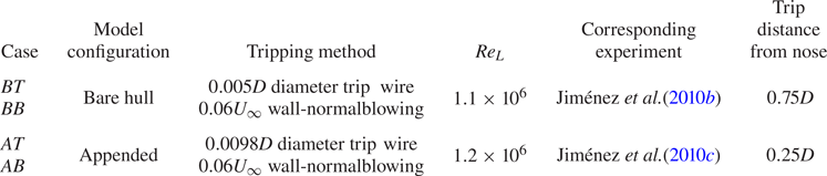
  $L$. These two cases correspond to the experiments of Jiménez et al. (Reference Jiménez, Hultmark and Smits2010b) and Jiménez et al. (Reference Jiménez, Reynolds and Smits2010c), respectively, each of which used different trip wire sizings and locations (as summarized in table 2). This variation of trip geometry permits the study of transition initiated inside and outside the boundary layer as well as the effects of pressure gradients and curvature on the post-trip TBL development. In addition to numerically resolving the trip wire geometry of the experiments, we also consider a simple numerical trip, which consists of a wall-normal blowing velocity of 0.06 $U_\infty$ imposed on the wall at the trip location, which promotes immediate transition by mimicking an array of wall-normal jets. Table 2 summarizes the parameters and designations of the four cases, with case BB referring to the LES results from Morse & Mahesh (Reference Morse and Mahesh2021). With these cases under consideration, we focus on three areas in the discussion of the results:
(i) the relaxation of the post-trip TBL to an ‘equilibrium’ state in terms of integral quantities, turbulence statistics and boundary layer structure;
(ii) the differences between the resolved trip wire and the artificial numerical trip; and
(iii) the influence of tripping the model appendages.
Table 2. Details of the four cases considered in the present study and their designations, where  $D$ is the hull diameter. Case BB corresponds to the simulation results from Morse & Mahesh (Reference Morse and Mahesh2021). Note that additional comparisons in the manuscript are made with the extensive suite of surface measurements from Huang et al. (Reference Huang, Liu, Groves, Forlini, Blanton and Gowing1992) and Liu & Huang (Reference Liu and Huang1998), which were performed at $Re_L = 1.2 \times 10^7$ with a $0.00125D$ trip wire placed $0.425D$ from the front of the hull.
The remainder of the paper is organized as follows. Section 2 reports the computational method and the simulation details. Section 3 reports the simulation results by walking through the local flow around the trip in § 3.1, the post-trip TBL recovery in §§ 3.2–3.4 and appendage tripping effects and the wake in §§ 3.5 and 3.6. Finally, § 4 concludes the paper.
2. Simulation details
The computational method is detailed in § 2.1 and the computational grid and domain sizing for each case is described in § 2.2.
2.1. Numerical method
Large-eddy simulations are performed using the unstructured overset method of Horne & Mahesh (Reference Horne and Mahesh2019a,Reference Horne and Maheshb) to solve the spatially filtered incompressible Navier–Stokes equations in the arbitrary Lagrangian–Eulerian frame
 \begin{gather} \frac{\partial \bar{u}_i}{\partial t} + \frac{\partial}{\partial x_j} (\bar{u}_i \bar{u}_j - \bar{u}_i {V}_j) ={-}\frac{\partial \bar{p}}{\partial x_i} + \nu \frac{\partial^2 \bar{u}_i}{\partial x_j \partial x_j} - \frac{\partial \tau_{ij}}{\partial x_j}, \end{gather}
 \begin{gather}\frac{\partial\bar{u}_i}{\partial x_i} = 0, \end{gather}
where  $u_i$ are the velocity components, $p$ is the pressure, the overbar denotes spatial filtering and $V_j$ is the mesh velocity, which is included in the convective term to avoid tracking of multiple reference frames for each overset grid. In the LES approach, the large energy-carrying scales are resolved, while the subgrid stress tensor, $\tau _{ij} = \overline {u_i u_j} - \bar {u}_i \bar {u}_j$, is modelled using the dynamic Smagorinsky model (Germano et al. Reference Germano, Piomelli, Moin and Cabot1991; Lilly Reference Lilly1992). The Lagrangian time scale is dynamically computed based on surrogate correlation of the Germano-identity error (Park & Mahesh Reference Park and Mahesh2009). This LES methodology has shown good performance for a propeller in crashback (Verma & Mahesh Reference Verma and Mahesh2012; Kroll & Mahesh Reference Kroll and Mahesh2022) and the bare hull DARPA SUBOFF (Kumar & Mahesh Reference Kumar and Mahesh2018b; Morse & Mahesh Reference Morse and Mahesh2021).
The above equations are solved using the finite-volume method of Mahesh, Constantinescu & Moin (Reference Mahesh, Constantinescu and Moin2004) for incompressible flows on unstructured grids, which emphasizes kinetic energy conservation to ensure robustness without added numerical dissipation. The method uses a second-order centred spatial discretization where the filtered velocity components and pressure are stored at the cell centroids and the face-normal velocities are stored independently at the face centres. A predictor–corrector method with a rotational correction incremental scheme (Guermond, Minev & Shen Reference Guermond, Minev and Shen2006) is used, and time advancement is accomplished with either Crank–Nicolson or second-order backward differencing implicit time integration. The multi-point flux approximation developed by Horne & Mahesh (Reference Horne and Mahesh2021) is used to construct accurate gradients on skewed meshes. This method was extended for overset computations by Horne & Mahesh (Reference Horne and Mahesh2019a,Reference Horne and Maheshb), which allows for the computational domain to be decomposed into a set of arbitrarily overlapping and moving meshes. Although there is no grid movement in the present case, the overset method greatly simplifies the grid generation process by allowing grids for the appendages and trip wire to be designed in isolation. This feature also permits the systematic study of tripping geometries.
2.2. Details of the computational set-up
Figure 3 shows a sketch of the computational domain for each configuration. The origin of the domain coincides with the nose of the hull, with the  $x$-axis extending along the length of the hull and the $y$-axis pointing in the direction of the sail for the appended cases. The $z$-axis follows to form a right-handed coordinate system. Following the grid confinement study of Kumar & Mahesh (Reference Kumar and Mahesh2018b), the radius of the computational domain is $6D$, the inflow boundary is placed a distance $3D$ from the nose of the hull and the outflow boundary is $17.2D$ from the stern, where $D$ is the maximum diameter of the hull. For reference, the length of the hull is $L = 8.6D$. Free-stream ( $u = U_\infty$, $v=w=0$) boundary conditions are prescribed at the inflow and lateral boundaries, while a convective boundary condition is imposed at the outflow. A no-slip boundary condition is used on the hull surface, and the boundary conditions at the edge of overset meshes are achieved by interpolation (Horne & Mahesh Reference Horne and Mahesh2019b).

Figure 3. Computational domain for simulation of the SUBOFF hull, where the background grid is shown in black, the wake refinement grid is in blue and the hull grid is shown in red. The background grid dimensions, boundary conditions and coordinate system are labelled. Panels (b,c) show the additional overset grids for the resolved trip (purple), sail (green) and stern appendages (fuchsia, aqua, yellow) which are selectively added to form the BT, AB and AT configurations.
As seen in figure 3, the overset method allows the domain to be split into multiple overset grids, which allows the model geometry to be configured by adding additional overset grids for the appendages and trip wires. Panels (b,c) of figure 3 depict the additional grids for the resolved trip and appended simulations, and figure 4 shows a  $z$-plane slice of the grids for case AT. Similarly to Torlak et al. (Reference Torlak, Jensen and Hadžić2005), the bottom of the trip wire geometry is squared off (see figure 4b) for cases BT and AT to prevent excessive skewness of the grid.
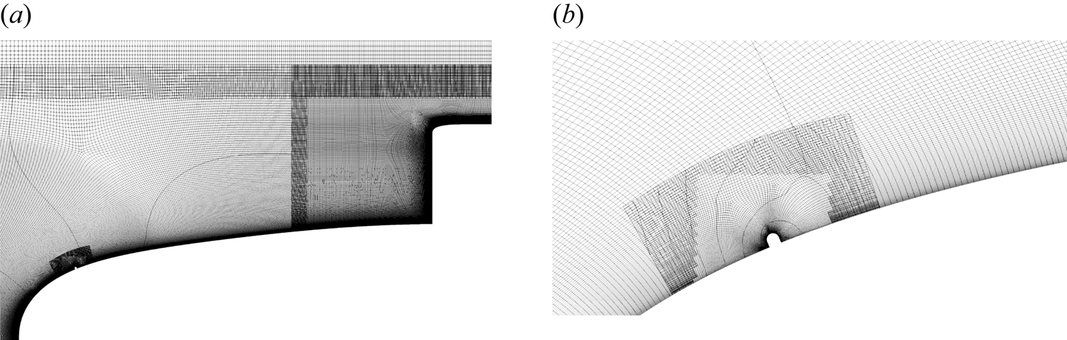
Figure 4. Symmetry plane ( $z$-plane) slices of the grids for case AT: (a) slice of the hull, sail, trip wire and background grids, and (b) zoomed-in view of the trip wire grid.
Table 3 summarizes the number of cells and processors for the overset grids associated with each case. The background, hull and wake refinement grids are identical to those used by Morse & Mahesh (Reference Morse and Mahesh2021) for wall-resolved LES of the bare hull, and the reader is referred to their paper for a detailed description of grid sizing and resolution. The nominal first cell spacings at the mid-hull in wall units are  ${\rm \Delta} x^+ = 33$, ${\rm \Delta} r^+ = 1$ and $a^+ {\rm \Delta} \phi = 11$, where $\phi$ is the azimuthal coordinate, $a^+ = a u_\tau / \nu$ and $a = D/2$ is the local radius of the body at the mid-hull. The additional grids for the sail, stern appendages and resolved trip wires are added selectively to form the BT, AB and AT cases. The blowing trip and resolved trip wire configurations are identical in the computational grid set-up besides the addition of the overset grid containing the trip wire geometry, while the other grids remain entirely unchanged.
Table 3. Details of the overset grids used for each simulation configuration, including number of control volumes and number of processors per grid.

The total number of control volumes ranges from 712 million for case BB to 843 million for case AT, with an associated processor count ranging from 9504 to 11 616 per case. Each case is run for a time of at least one flow-through time ( $t = 28.8D/U_\infty$) to discard initial transients before collecting boundary layer statistics. Statistics are collected for another two flow-through times. For case BB, the non-dimensional timestep is ${\rm \Delta} t U_\infty /L = 1.4 \times 10^{-4}$, while case BT is limited to half this timestep due to the fine resolution near the trip wire. Similarly, case AB uses a non-dimensional timestep of $7 \times 10^{-5}$, while case AT requires $4.9 \times 10^{-5}$. The maximum timestep in inner units at the mid-hull across all cases is ${\rm \Delta} t^+ < 0.33$, which is adequate to capture the near-wall dynamics of the TBL. The computations were carried out on a Cray XC40/50 cluster with 2.8-GHz Intel Xeon Broadwell cores and an HPE Cray EX system with 2.3-GHz AMD EPYC 7H12 processors. The total cost of the computations exceeded 30 million CPU hours.
3. Results and discussion
Figure 5 shows contours of instantaneous velocity in the  $z$-plane for cases BT and AT. The complexity of the flow is apparent from the thin boundary layer developing along the hull before thickening at the stern, the wakes of the sail and stern appendages and the slow development of the wake. The tripping location for each configuration is marked with arrows, but the trip wire itself remains imperceptible, highlighting the disparity in scales between the trip wire and the hull geometry.

Figure 5. Contours of instantaneous velocity magnitude normalized by  $U_\infty$ in the $z$-plane for case BT (a) and AT (b). The location of the trip wire for each case is marked with arrows.
In order to present the analysis of tripping effects for each configuration, we move from the bow to the stern of the model, focusing first on the surface quantities and local flow around the trip in § 3.1, followed by the TBL recovery after the trip in § 3.2 and the lasting effects of the trip on integral quantities and the mid-hull TBL in §§ 3.3 and 3.4. Finally, the importance of tripping effects on the sail and stern appendages is discussed in § 3.5, and the wake statistics are presented in § 3.6.
3.1. Surface quantities and local flow around the trip
We first start with analysis of the flow field around the trip wire and the subsequent development of the TBL along the mid-hull. Figure 6 shows the evolution of the pressure and skin friction coefficients, defined respectively as
 \begin{equation} C_p = \frac{P - P_\infty}{\frac{1}{2} \rho U_\infty^2},\quad C_f = \frac{\tau_w}{\frac{1}{2} \rho U_\infty^2}, \end{equation}
along the hull for all four cases, where  $P$ and $\tau _w$ are the mean pressure and shear stress at the wall, $\rho$ is the density and $P_\infty$ and $U_\infty$ are the free-stream pressure and velocity, respectively. Note that data for the appended hull have been taken from the side of the hull opposite the sail from the nose to where the hull begins to taper. Also shown in figure 6 are the experimental data for the bare hull from Huang et al. (Reference Huang, Liu, Groves, Forlini, Blanton and Gowing1992) at $Re_L = 1.2 \times 10^7$. Despite the difference in Reynolds number, the $C_p$ from the simulations agrees well with the experimental data of Huang et al. (Reference Huang, Liu, Groves, Forlini, Blanton and Gowing1992) for the length of the hull due to the lack of sensitivity of $C_p$ to Reynolds number ( $Re$) at high- $Re$. Only at the last section of the stern do the differences in $Re_L$ become appreciable, since at this point boundary layer thickness effects become significant.

Figure 6. Profiles of (a)  $C_p$ and (b) $C_f$ along the hull for cases BT ( $\cdot \!\cdot \!\cdot \!\cdot \!\cdot \!\cdot \!\cdot \!\cdot$, green), BB (——–, blue), AT ( $\cdot \!\cdot \!\cdot \!\cdot \!\cdot \!\cdot \!\cdot \!\cdot$, violet), AB (——–, red) and from the wall-resolved LES of Posa & Balaras (Reference Posa and Balaras2016) ( $\bullet$, grey), where the appended data have been taken from the side opposite the sail before the stern begins to taper. Insets show zoomed-in views of the same axes near the trip, where the appended and bare hull trip positions are marked on the abscissa with $A$ and $B$, respectively. The slope of $C_f$ for a zero-pressure-gradient flat-plate TBL (Schlichting Reference Schlichting1968) is shown in (b) for the mid-hull (– – – –). Experimental data from Huang et al. (Reference Huang, Liu, Groves, Forlini, Blanton and Gowing1992) ( $\square$) are also shown, with the experimental $C_f$ data scaled to the $Re$ of the appended simulations using $C_f \sim Re^{-1/5}$.
Posa & Balaras (Reference Posa and Balaras2016) performed wall-resolved LES of the appended hull at  $Re_L = 1.2 \times 10^6$, matching the conditions of cases AT and AB. These authors performed their computations using an immersed boundary method and applied a volume force to a few cells near the wall to simulate the trip at the same position ( $x/D = 0.25$) as cases AT and AB. Their well-documented statistics provide a useful point of comparison for the present computations. The pressure coefficient from the present results agrees well with Posa & Balaras (Reference Posa and Balaras2016) besides exhibiting a slightly higher pressure over the mid-hull, most likely due to the more confined radial boundary of Posa & Balaras (Reference Posa and Balaras2016) ( $r = 4.3D$) vs the present computations ( $r = 6D$).
The tripping location for each configuration is clearly visible from the spikes in pressure around the trip, which is magnified in the inset of figure 6(a). The pressure coefficient near each of the resolved trip wires (cases BT and AT) is characterized by a pressure rise associated with the flow stagnation in front of the trip, followed by a rapid drop in pressure and an extended region of suction behind the trip wire. Following this point, there is an elevation of  $C_p$ above the nominal curve, which will be shown to be related to the reattachment point of a recirculation bubble behind the trip wire. After this point, the curves recover to the nominal pressure evolution along the hull. The elevation of the stagnation pressure above the nominal $C_p$ curve associated with the trip wire for case AT is four times that of case BT, and nearly eliminates the region of suction over the bow, which may affect the form drag of the hull. In the region behind the trip, the depression of $C_p$ for case AT is nearly three times that of case BT. For cases BB and AB with the blowing tripping strategy, there is also a rise in $C_p$ in front of the trip followed by a sharp drop after the trip. The pressure peak in front of the trip for case BB is nearly the same magnitude as case BT, but the peak for case AB is much lower than that of case AT. Additionally, the drop in pressure behind the trips for both cases BB and AB is lower in magnitude than for either case BT or AT and there is no pressure rise above the nominal curve after this low pressure region. Instead, the curves quickly converge back to the normal $C_p$ development along the hull. Overall, the recovery length for $C_p$ behind the resolved trip wire is over double that of the blowing trip.
Next, the skin friction coefficient is compared with the measurements of Huang et al. (Reference Huang, Liu, Groves, Forlini, Blanton and Gowing1992) at  $Re_L = 1.2 \times 10^7$ (figure 6b). Due to the differences in Reynolds number between the simulations and the experiment, we apply $C_f \sim Re^{-1/5}$ scaling for high- $Re$ attached ZPGTBLs to scale the experimental data to the Reynolds number of cases AT and AB. While this scaling is only valid for the ZPG parallel mid-section of the hull, we observe good agreement between the LES and experiment. The slope of the $C_f$ evolution on the mid-hull also agrees well with that of Schlichting (Reference Schlichting1968).
Focusing near the tripping location, we see that the development of  $C_f$ for the resolved trip wires is characterized by a drop in $C_f$ in front of the stagnation point imposed by the trip wire, followed by a spike in $C_f$ over the trip itself. For case AT, the trip wire induces a small separation bubble ahead of the wire, resulting in a slightly negative $C_f$ value in this region. Following the trip location, the separation bubble behind the trip appears as an extended region of negative $C_f$, which is longer for case BT compared with case AT, despite the smaller trip wire diameter. This is likely due to the difference in local pressure gradients between the two trip positions. Figure 7(a,b) shows mean streamlines around the trip location for cases BT and AT, where the recirculation bubble is clearly visualized by the coloured streamlines. At the reattachment point of the recirculation bubble, there is a spike in $C_f$, followed by a region of elevated $C_f$ above the blowing cases that persists longer than the recovery length for the pressure coefficient. Compared with cases BT and AT, the simulations with the blowing trip strategy do not induce as large a drop in $C_f$ ahead of the trip and no recirculation region of negative $C_f$ is observed behind the tripping location. This is verified by the mean streamlines in figure 7(c,d), which show a mean ejection from the wall for the blowing tripping strategy. For these cases, the numerical trip produces a slight lifting of the near-wall streamline but not to the same extent as the deflection of the streamlines over the trip wire in cases BT and AT. The spike in skin friction behind the trip is also underpredicted by both blowing trip cases when compared with the resolved simulations.

Figure 7. Mean streamlines in the  $z=0$ plane for case BT (a), AT (b), BB (c) and AB (d). Coloured streamlines highlight local flow differences between resolved trip wire and blowing trip configurations. The wall-parallel coordinate, $s$, is also depicted.
Finally, the results of Posa & Balaras (Reference Posa and Balaras2016) show a quite different evolution of the skin friction behind the trip wire, which may indicate differences due to the volume-forcing tripping strategy. The peak in  $C_f$ is delayed to $x/L \approx 0.2$, indicating that the state of the inner layer is different from the present computations. However, the agreement of the present $C_f$ with that of Posa & Balaras (Reference Posa and Balaras2016) on the mid-hull is excellent. This indicates that the inner layer for each case is able to recover to a similar state given adequate streamwise distance, as observed for tripping of flat-plate ZPGTBLs (Erm & Joubert Reference Erm and Joubert1991; Schlatter & Örlü Reference Schlatter and Örlü2010; Marusic et al. Reference Marusic, Chauhan, Kulandaivelu and Hutchins2015; Kozul et al. Reference Kozul, Chung and Monty2016).
3.1.1. Local flow structure around the trip
To explore the flow around the trip in detail, figure 8 shows mean velocity profiles in  $s$-
$s$- $n$ coordinates around the trip for all four cases. In this coordinate system, $s - s_t$ is the wall-parallel distance from the trip location, as shown in figure 7, $n$ is the wall-normal direction and $U_s$ is the wall-parallel mean velocity. The incoming boundary layer for each case is laminar, and the edge of the boundary layer is marked with symbols. The boundary layer edge (and boundary layer thickness, $\delta$) are identified using the $0.99 C_{p_{tot},\infty }$ total pressure metric suggested by Patel, Nakayama & Damian (Reference Patel, Nakayama and Damian1974), which was shown to be appropriate for the bare hull SUBOFF by Morse & Mahesh (Reference Morse and Mahesh2021). Note that this definition reduces to the typical $0.995 U_\infty$ metric on the mid-hull, where pressure variations across the boundary layer are minimal. For case BT, the incoming boundary layer is thicker than the trip diameter (figure 8a), while the trip height is taller than the boundary layer thickness for case AT. The ratio of the trip diameter to the boundary layer thickness (measured at a station $5d$ in front of the trip) is $d/\delta = 0.45$ for case BT and $d/\delta = 1.92$ for case AT. Additionally, based on the velocity profile at $5d$ in front of the trip wire, case BT has a trip Reynolds number of approximately $Re_d \approx 390$, whereas $Re_d \approx 1330$ for case AT. Guidance from flat-plate tripping studies suggests that the value for case AT would lead to over-tripping behaviour. However, given the local pressure gradient at this tripping location, this conjecture must be verified.

Figure 8. Profiles of  $U_s/U_\infty$ for cases BT and BB (a) and AT and AB (b), where symbols denote the boundary layer edge.
For both resolved trip configurations, the boundary layer ahead of the trip decelerates to stagnate in front of the trip wire, which is not reflected in the trip simulations using the numerical tripping strategy. A region of high shear is formed above the trip wire, and a recirculation bubble is produced that is less than 8 trip diameters in length for case AT and more than 16 trip diameters long for case BT. The post-tripping boundary layer thickness for cases BT and BB are relatively similar, although the resolved trip produces a slightly thinner boundary layer after the reattachment point of the recirculation bubble. In contrast, the symbols in figure 8(b) reveal that the boundary layer thickness for case AT jumps up to approximately double that of case AB directly behind the trip, due to the large  $d/\delta$. This difference persists to the last station, where the boundary layer for case AT is substantially thicker than for the blowing trip.
Figure 9 shows profiles of turbulent kinetic energy (TKE),  $k = \frac {1}{2} \overline {u_i u_i}$, in the same coordinate system. Contours of TKE production, $\mathcal {P} = - \overline {u_s u_n} ({\partial U_s}/{\partial n})$, are also plotted in the same figure. The resolved trip wire cases show zero turbulence intensity ahead of the trip wire, while the blowing trip computations do show some unsteadiness ahead of the tripping location. This is due to non-uniformities in the grid cells where tripping is introduced, which require that the wall normal blowing velocity is applied to centres of wall boundary faces that fall within $0.744 < x/D < 0.756$ for case BB and $0.246 < x/D < 0.258$ for case AB. For the resolved trip in case BT, we observe no turbulence at the first station downstream of the trip wire, following which $k$ slowly grows along the shear layer and within the recirculation bubble 10 diameters downstream of the trip wire. It is only near the reattachment point of the recirculation bubble that $k$ peaks to values exceeding those for case BB, which aligns with the argument of Preston (Reference Preston1958) that for a trip wire, unsteadiness at the reattachment point should produce the disturbance to promote transition, as opposed to shedding from the trip itself. This is confirmed by the contours of $\mathcal {P}$ for case BT, which show that TKE production peaks near the reattachment point. While production is delayed for case BT compared with case BB, the bands of production are relatively well aligned by $(s-s_t)/d = 20$.

Figure 9. Profiles of  $50k/U_\infty ^2$ for cases BT and BB (a) and AT and AB (b), where symbols denote the boundary layer edge. Contours of production for each case are also shown at levels $\mathcal {P} (D / U_\infty ^3) = 0.15, 0.3$.
For case AT, the behaviour behind the trip wire is significantly different. The magnitude of  $k$ exceeds that of case AB at the first profile downstream of the trip wire, and location of peak $k$ highlights that this turbulence is associated with shedding from the trip wire. This indicates an over-tripped condition, and is associated with a peak of TKE production immediately behind the top of the trip wire. In contrast to cases BT, BB and AB, where turbulence is initiated within the boundary layer, the shedding behind the trip for case AT induces turbulence away from the wall, which leads to a rapid increase in the boundary layer thickness. This is highlighted by the separation of the TKE production contours for cases AT and AB. Moving along the edge of the shear layer, values of $k$ for case AT are up to four times those of the other cases (noting that the scale of $k$ profiles in figure 9(a,b) are identical). By 20 diameters downstream of the trip wire, the profiles of $k$ have subsided to values closer to those of the other configurations, but the boundary layer has been rapidly thickened by this stage. The peak of $k$ near the wall and the contours of production appear at a similar position to those for case AB, but the upstream TKE production near the top of the trip has led to a long tail in the profile of $k$, which stretches to the edge of the boundary layer.
3.2. Post-trip boundary layer recovery
Following the trip, a TBL evolves along the hull and recovers from its initial tripped state. Figure 10 shows contours of instantaneous wall-parallel velocity for each case on a surface offset from the hull by one trip diameter. In this view, the local differences between the trip configurations are apparent, and the recirculation bubble for case BT is clearly visible. Following the tripping location, the near-wall streaks are quickly developed for cases BT and BB. In contrast to the recirculation bubble for case BT, the region immediately downstream of the trip for case AT is highly turbulent and has visibly less spanwise coherence. Since the trip wire for the appended hull cases is nearly double the size of the bare hull trip wire, the surface offset distance from the hull is larger for the appended cases. Therefore, turbulence is not immediately visible downstream of the trip for case AB, although figure 9 confirms that transition is indeed initiated immediately at the trip location near the wall. Again, due to the larger distance of the offset surface from the wall, the near-wall streaks for the appended cases do not appear until the mid-hull, at which point the low and high momentum regions induced by the sail junction vortex are apparent.

Figure 10. Contours of instantaneous wall-parallel velocity normalized by  $U_\infty$ for case BT (a), BB (b), AT (c) and AB (d) plotted against the wall-parallel distance and azimuthal angle in degrees ( $\phi$) on a surface at a constant offset of one trip diameter from the hull surface. Note that this offset is $0.005D$ for cases BT and BB vs $0.0098D$ for cases AT and AB. Dashed lines are plotted at intervals of $r\phi /D = 0.25$ to highlight the changing local radius of the hull.
The evolution of the friction Reynolds number,  $Re_\tau = u_\tau \delta / \nu$ (where $u_\tau = \sqrt {\tau _w / \rho }$ is the friction velocity), and $Re_\theta$ are presented in figure 11. Clearly, $Re_\theta < 2000$ for each case (besides Posa & Balaras Reference Posa and Balaras2016), so the boundary layers at the present $Re_L$ are well within the moderate Reynolds number range and history effects of tripping may be significant. Notably, the trip location for both the bare hull and appended cases is below the critical $Re_\theta$ for the convective instability of the Blasius boundary layer ( $Re_\theta < 200$), so the trips must either induce an absolute instability or modify the base flow to alter the critical Reynolds number. The challenge of avoiding over-tripping is more difficult for the trip location in case AT, and the present results show that the boundary layer has been over-tripped. The different $Re_\tau$ between the tripping configurations of each geometry are due to the differences in $\delta$ and $C_f$, while the differences in $Re_\theta$ must be due to differences in $\theta$, which will be explored in detail. The growing disparity in the local Reynolds numbers between the appended and bare hull cases is a result of the slightly different $\nu$, a result of the small difference in $Re_L$.

Figure 11. Evolution of  $Re_\tau$ (a) and $Re_\theta$ (b) along the hull (appended data have been taken from the side opposite of the sail, $y<0$). The LES results from Posa & Balaras (Reference Posa and Balaras2016) are shown as grey dots. The location of the trip wire for the appended and bare hull cases are marked on the abscissa with $A$ and $B$, respectively.
3.2.1. Boundary layer profiles
The recovery of the boundary layer is investigated in more detail by examining profiles downstream of the tripping location. Figure 12 shows profiles of  $U_s$ with inner and outer (defect) scaling at three locations spaced $0.3D$, $0.9D$ and $2.7D$ downstream of the trip. For cases BT and BB, the log law quickly sets up by $(s-s_t)/D = 0.3$, at which point the local difference in skin friction manifests as a larger $U_e^+$ for case BB. By $2.7D$ downstream of the trip, the profiles of $U_s$ have collapsed in both inner and outer scaling. At the intermediate station, the offset to the log law (figure 12a) is due to the local streamwise pressure gradient. The corresponding profiles of $\overline {u_s^2}$ are shown in figure 12(c), where we see that turbulence in the inner layer collapses quite quickly after the trip, despite small differences in the peak value at the first two stations.

Figure 12. Profiles of  $U_s$ in inner scaling (a,d) and defect form (b,e) along with $\overline {u_s^2}$ and $\overline {u_n^2}$ in inner scaling (c,f) for cases BT and BB (a–c) and cases AT and AB (d–f). Note the shift in ordinate for profiles at stations $(s-s_t)/D = 0.3$, 0.9, and 2.7. Line styles match those described in figure 6, while profiles for $\overline {u_n^2}$ are translucent, and the log law is shown with black lines in (a,d).
The profiles of  $U_s$ for cases AT and AB are shown in the same figure, where the differences to the log law are more apparent at the first station. By the last station, the profile of $U_s$ has collapsed in the inner layer, but shows some differences in the outer layer. This is confirmed by the corresponding profile in figure 12(e), which does not show the collapse achieved by the bare hull simulations at the third station. Examining $\overline {u_s^2}$ for the appended cases shows greater differences in the inner layer at the first station than for the bare hull cases, with the peak showing a lower magnitude for case AT than for case AB. This is peculiar given the larger peak observed for the over-tripped flat-plate ZPGTBL from Marusic et al. (Reference Marusic, Chauhan, Kulandaivelu and Hutchins2015), and may be due to the effect of the trip on the local pressure gradient. Compared with the bare hull cases, the shape of the $\overline {u_s^2}$ profile shows much greater differences between cases AT and AB, especially close to the edge of the boundary layer, where differences persist to the last station. Even greater differences are observed in the profiles of $\overline {u_n^2}$ (shown as translucent lines in figure 12c,f) for case AT. Whereas the profiles of $\overline {u_n^2}$ for the bare hull cases show a similar collapse to $\overline {u_s^2}$, for the appended cases, the resolved trip results in a large peak of $\overline {u_n^2}$ away from the wall, which is associated with the shedding from the trip wire. The wall-normal and wall-parallel turbulence intensities appear to recover by the same station, as reported by Schlatter & Örlü (Reference Schlatter and Örlü2012) for a flat-plate ZPGTBL.
3.2.2. Mean momentum balance
The mean momentum balance (MMB) of the boundary layer approximation of the Reynolds-averaged Navier–Stokes equations has proven to be a valuable tool in the study of boundary layer structure (Wei et al. Reference Wei, Fife, Klewicki and McMurtry2005; Morrill-Winter, Philip & Klewicki Reference Morrill-Winter, Philip and Klewicki2017), as well as transitional and pressure gradient boundary layers (Klewicki, Ebner & Wu Reference Klewicki, Ebner and Wu2011; Romero et al. Reference Romero, Zimmerman, Philip, White and Klewicki2022). A natural frame in which to analyse the MMB for streamwise curvature was suggested by Morse & Mahesh (Reference Morse and Mahesh2021), which considers the balance in a  $\xi$- $\eta$ coordinate system, made up of streamlines ( $\xi$-direction) and streamwise-normal lines ( $\eta$-direction). The boundary layer approximation of the axisymmetric mean momentum equations in the $\xi$- and $\eta$-directions are given by
 \begin{gather} \overbrace{U_\xi \frac{\partial U_\xi}{\partial \xi}}^{{\rm MI}} + \overbrace{\frac{1}{\rho} \frac{\partial P}{\partial \xi}}^{{\rm PG}_\xi} + \overbrace{\frac{1}{r} \frac{\partial}{\partial \eta} \left( r \overline{u_\xi u_\eta} \right)}^{{\rm TI}} + \overbrace{\frac{1}{r} \frac{\partial}{\partial \eta} \left({-}r \nu \frac{\partial U_\xi}{\partial \eta} \right)}^{{\rm VF}} = 0, \end{gather}
 \begin{gather}\underbrace{\frac{U_\xi^2}{R_\xi}}_{{\rm CA}} + \underbrace{\frac{1}{\rho} \frac{\partial P}{\partial \eta}}_{{\rm PG}_\eta} + \underbrace{\frac{1}{r} \frac{\partial}{\partial \eta} \left(r\overline{u_\eta^2} \right)}_{{\rm NF}} = 0, \end{gather}
where we see that writing the equations in this frame simplifies the mean inertia (MI) term and introduces a centripetal acceleration (CA) term to account for streamline curvature. As a result, the streamwise momentum equation is a balance between MI, the streamwise pressure gradient (PG $_\xi$), the turbulent inertia (TI) and the viscous force (VF). The streamwise-normal balance is between CA, the streamwise-normal pressure gradient ( ${\rm PG}_\eta$) and the gradient of the streamwise-normal turbulent stress (NF).
Figures 13 and 14 show the MMB for the bare hull and appended tripping configurations, respectively, at locations  $(s-s_t)/D = 0.3$, 0.9, 2.7 (the same locations considered in figure 12). While the BT and BB configurations show small differences in the MMB terms at the first station, these differences are mainly limited to the peaks of the TI and MI terms, although a difference in the streamwise pressure gradient is visible. The differences between the terms are even more minimal for the streamwise-normal MMB in figure 13(d), and by the third station the momentum balance has collapsed in both the streamwise and streamwise-normal directions.


In contrast, figure 14(a,d) shows large differences in both the streamwise and streamwise-normal MMBs at the first station. We see that the streamwise pressure gradient is much smaller for case AT, which, in combination with the changes to the tail of the Reynolds shear stress term (TI), causes a reduction in the magnitude of the MI term. This would suggest a slower growth of the momentum thickness directly downstream of the trip for case AT. Figure 14(d) displays stark differences in the streamwise-normal MMB, with peaks of the NF and  ${\rm PG}_\eta$ terms for case AT that are over double those for case AB, while the CA term is of a similar magnitude. This is due to a significant modification of the streamwise-normal Reynolds stress directly downstream of the trip wire for case AT, as observed in figure 12(f). The differences in the streamwise and streamwise-normal MMBs have started to collapse by the second station, with the largest differences between the tripping configurations being the reduction of the strength of the momentum sink for case AT due to the reduced TI peak away from the wall. By the final station, however, the MMB has mostly collapsed between the AT and AB tripping configurations, suggesting that the boundary layer should develop in a similar manner by this point on the mid-hull.
3.2.3. Anisotropies
Given the differences observed in the boundary layer profiles and structure between tripping configurations, it naturally follows to assess the state of the turbulence in the TBL. A popular method to characterize turbulence is through anisotropy invariant maps, as proposed by Lumley & Newman (Reference Lumley and Newman1977). These two-dimensional maps are based on the eigenvalues ( $\lambda _i$) of the turbulence anisotropy tensor
 \begin{equation} a_{ij} = \frac{\overline{u_i u_j}}{2k} - \frac{\delta_{ij}}{3}, \end{equation}
where  $\delta _{ij}$ is the Kronecker delta. Banerjee et al. (Reference Banerjee, Krahl, Durst and Zenger2007) suggested the use of a barycentric map to visualize these eigenvalues, in which the coordinates $(x_B,y_B)$ of the mapping are given by
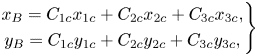 \begin{equation} \left.\begin{gathered} x_B = C_{1c} x_{1c} + C_{2c} x_{2c} + C_{3c} x_{3c}, \\ y_B = C_{1c} y_{1c} + C_{2c} y_{2c} + C_{3c} y_{3c}, \end{gathered}\right\} \end{equation}
where  $(x_{ic},y_{ic})$ are the coordinates of the corners of the triangle and coefficients of the map are
 \begin{equation} C_{1c} = \lambda_1 - \lambda_2,\quad C_{2c} = 2 \left( \lambda_2 - \lambda_3 \right),\quad C_{3c} = 3 \lambda_3 + 1. \end{equation}
The three limiting states of turbulence are the one-component (1C) limit (‘rod-like’ turbulence), the axisymmetric two-component (2C) limit (‘disk-like’ turbulence), and the three-component (3C) isotropic limit, as labelled in figure 15. The boundaries of the map consist of the lines drawn between these points, and represent the two-component turbulence, axisymmetric contraction and axisymmetric expansion limits. The plane strain line exists within the map and occurs when at least one of the eigenvalues is zero.

Figure 15. Barycentric map of the anisotropy along wall-normal lines for cases BT and BB (a–c) and AT and AB (d–f), at the same locations as the profiles presented in figure 12. Points on the map are shaded by distance from the wall.
Figure 15 plots the anisotropies along wall-normal lines for each case at the same locations as the profiles in figure 12 ( $0.3D$, $0.9D$ and $2.7D$ downstream of the trip). For cases BT and BB, the anisotropy at the first profile downstream of the trip has collapsed in the inner layer near the wall, and the behaviour near the edge of the boundary layer is visually similar. By the second station, the profiles have achieved a reasonable collapse across the entire boundary layer, and the profiles lie nearly perfectly on top of each other by the final station.
In contrast, for cases AT and AB, the profiles do not show any such collapse for the first station, at which point neither the inner nor outer layers match between the tripping configurations. This indicates that the state of the turbulence is remarkably different in proximity to the trip. This difference persists away from the wall to the second station, although the turbulence near the wall is similar between the cases. By the final station, small differences still persist in the outer layer, although the inner layer has fully collapsed.
3.3. Integral quantities
The lasting effect of the trip on the hull TBL is best understood by investigating the evolution of the TBL integral quantities. Despite the seemingly quick collapse of  $C_p$ and $C_f$ between tripping configurations in figure 6 and the slow recovery of the TBL in § 3.2, the integral state of the TBL shows notable differences which persist over the length of the hull.
3.3.1. Boundary layer thicknesses
Figure 16 shows the evolution of  $\delta$, $\delta ^*$ and $\theta$ along the surface of the hull on the side opposite of the sail ( $y<0$). The displacement and momentum thicknesses are calculated using the planar definitions as
 \begin{equation} \delta^* = \int_0^\delta \left( 1 - \frac{U_s}{U_e} \right) {\rm d} n,\quad \theta = \int_0^\delta \frac{U_s}{U_e} \left( 1 - \frac{U_s}{U_e} \right) {\rm d} n, \end{equation}
where  $U_e$ is the wall-parallel velocity at the edge of the boundary layer ( $n=\delta$). The evolution of these quantities displays the lasting effect that the tripping method has on the hull boundary layer. Figure 16 shows that the laminar boundary layer on the bow has identical properties between cases BT and BB until the trip position, labelled as $B$ on the horizontal axis. This is also true of cases AT and AB, for which the tripping location is labelled as $A$. For case BT, there is a small jump in $\delta$ at the trip location followed by a slight depression corresponding to the reattachment point. In contrast, for case AT, the increase in $\delta$ at the trip is over four times that of case BT, although the dip in thickness at the reattachment point is still present. After this point, the TBL thickens at an increased rate compared with the laminar boundary layer. For cases BB and AB, the jump in $\delta$ following the trip is similar to that of case BT, although there is no dip in $\delta$ due to the lack of a recirculation bubble behind the blowing trip.

Figure 16. Evolution of  $\delta$ (a), $\delta ^*$ (b) and $\theta$ (c) along the hull (appended data have been taken from the side opposite of the sail, $y<0$). The LES results from Posa & Balaras (Reference Posa and Balaras2016, Reference Posa and Balaras2020) are shown as grey dots and $\delta$ computed using the method of Griffin et al. (Reference Griffin, Fu and Moin2021) is shown with translucent lines in (a). Slopes of $\delta$, $\delta ^*$ and $\theta$ for a zero-pressure-gradient flat-plate TBL (Schlichting Reference Schlichting1968) are also shown (– – – –). The location of the trip wire for the appended and bare hull cases are marked on the abscissa with $A$ and $B$, respectively.
The tripping location is more apparent from the jump in  $\delta ^*$ in figure 16(b), which appears much more severe for the resolved trip cases due to the negative velocities in the recirculation bubble. Moving past the vicinity of the trip to the mid-hull, $\delta ^*$ for each case appears to evolve at a similar rate, but with an offset in thickness. For case BT, the boundary layer remains slightly thinner than that of case BB, while the boundary layer is substantially thicker for case AT compared with case AB. An offset is also observed when plotting the $\delta ^*$ from the LES results published by Posa & Balaras (Reference Posa and Balaras2020) for the appended hull. The displacement thickness immediately after the trip is quite similar between Posa & Balaras (Reference Posa and Balaras2020) and case AT, but the subsequent evolution shows a persisting offset. The same trend is observed for $\theta$ after the trip in figure 16(c), where the $\theta$ from Posa & Balaras (Reference Posa and Balaras2016) is offset from the $\theta$ of cases AT and AB. Despite this disparity, the evolution of $\theta$ along the hull follows a similar curve as cases AT and AB, matching the slope for a zero-pressure-gradient flat-plate TBL (Schlichting Reference Schlichting1968) over the mid-hull. Marusic et al. (Reference Marusic, Chauhan, Kulandaivelu and Hutchins2015) also found that $Re_\theta$ for different tripping conditions evolved at a similar rate for a flat-plate ZPGTBL, although the log–log plotting of their data masks the persisting offset in $Re_\theta$. The use of flat-plate TBL correlations for comparison is acceptable given that the ratio of $\delta$ to the maximum hull radius remains within the range $0.09 \leq \delta /a \leq 0.27$ for all cases over the mid-hull. Note that the specifics with which $\delta ^*$ and $\theta$ are calculated (integration bounds and radial vs wall-normal profiles) are not provided by Posa & Balaras (Reference Posa and Balaras2016, Reference Posa and Balaras2020), and as such, they may influence these integral values. However, these effects are expected to be most pronounced over the bow and relatively negligible for the parallel mid-hull ( $0.233 \leq x/L \leq 0.745$), permitting comparison with these external simulations.
Examining more closely the offset in  $\theta$ between the different tripping configurations, we find that the offset in $\theta$ between the resolved trip wire and blowing trip configurations levels out to be nearly constant with $x$ after $x/L > 0.25$, with $\theta$ for case BT below that of case BB and the opposite behaviour for cases AT and AB (figure 16c). Despite this constant disparity, the relative difference in $\theta$ between cases gradually diminishes with $x$ due to the growth of $\theta$ due to momentum loss along the hull. Specifically, the relative difference in momentum thickness between case AT and AB is nearly 140 % immediately after the trip, but declines to less than 6 % by $x/L = 0.75$. The per cent difference between cases BT and BB is smaller than for the appended hull, and decreases with $x$ to less than 2 % by $x/L = 0.75$. This is because the direct contribution of the trip to the total momentum thickness decreases along the hull as the integrated contribution of skin friction becomes an increasing fraction of the momentum thickness. This implies that, given sufficient development distance, the differences between tripping methods would lead to diminishing relative differences in boundary layer thickness for models at large $Re_L$, corresponding to large- $Re_\theta$ TBLs.
In contrast to the similar slopes of the  $\delta ^*$ and $\theta$ development between the simulations, the rate of development of $\delta$ exhibits differences based on the tripping method. While the post-trip $\delta$ for cases BT and BB appear to collapse before $x/L = 0.2$, they begin to diverge after this point before developing at a similar rate over the mid-hull with a small offset. The $\delta$ for case AT is much larger than that for case AB immediately after the trip, but $\delta$ for case AT grows at a slower rate than any of the other cases over the mid-hull, such that the offset between case AT and the other cases has diminished by the end of the mid-hull. To demonstrate that this is not an artifact of the method to find the boundary layer edge, we also show $\delta$ determined by the method of Griffin, Fu & Moin (Reference Griffin, Fu and Moin2021) with translucent lines in figure 16(a), which shows the same result. This difference in the evolution of $\delta$ suggests that the boundary layer for case AT is not in a canonical state as a result of over-tripping, which will be explored in more detail in the following sections.
The results of these tripping configurations for wall-resolved LES of matched geometry and  $Re_L$ clearly demonstrate that the differences in tripping method lead to offsets in $\delta$, $\delta ^*$, and $\theta$ that are carried along the remainder of the hull. While the offset in momentum thickness between tripping configurations may be insignificant in the context of a flat-plate TBL, where the local $Re_\theta$ is used to compare datasets, this offset in $\theta$ is important for flow around a model geometry, where there is an imposed external length scale arising from the model geometry.
3.3.2. Shape factor
The development of the shape factor,  $H = \delta ^*/\theta$, is shown in figure 17(a). For each case, the shape factor reduces from levels typical of laminar boundary layers before the trip ( $H$ varying around 2.59 due to local pressure gradients on the bow) to those typical of TBLs after the trip location, although the evolution of $H$ is different for each configuration. For cases BT and AT, there is a spike in $H$ directly behind the tripping location followed by a sharp drop off. However, for case AT, this drop is accompanied by a local minimum in $H$, which is not present for case BT. Examining case BB, we see that the numerical tripping method does not reproduce the spike in $H$ behind the trip, but agrees well with the evolution of $H$ after falling to values around 1.3. In contrast, case AB does not match the experimental trip results as well even after the rapid reduction of $H$ following the trip, and it takes until $x/L > 0.3$ for the shape factor curves to begin to meet again. This depression of the shape factor also seems to appear for over-stimulated flat-plate ZPGTBLs (Erm & Joubert Reference Erm and Joubert1991; Schlatter & Örlü Reference Schlatter and Örlü2012; Marusic et al. Reference Marusic, Chauhan, Kulandaivelu and Hutchins2015). The volume forcing trip of Posa & Balaras (Reference Posa and Balaras2016) mimics the effect of the trip wire better than the wall-normal blowing trip (case AB), likely due to the solid blockage effect. In contrast, case BB mimicked the BT tripping adequately, since transition is initiated below the edge of the boundary layer for the bare hull cases.

Figure 17. Evolution of shape factors  $H = \delta ^*/\theta$ (a) as well as $\delta /\delta ^*$ (translucent) and $\delta /\theta$ (b) along the hull (appended data have been taken from the side opposite of the sail, $y<0$). The LES results from Posa & Balaras (Reference Posa and Balaras2016, Reference Posa and Balaras2020) are shown as grey dots. The slope of $H$ for a zero-pressure-gradient flat-plate TBL (Chauhan, Monkewitz & Nagib Reference Chauhan, Monkewitz and Nagib2009) is also shown (– – – –). The location of the trip wire for the appended and bare hull cases are marked on the abscissa with $A$ and $B$, respectively.
Schlatter & Örlü (Reference Schlatter and Örlü2012) suggested that  $\delta /\delta ^*$ and $\delta /\theta$ were more sensitive indicators of the state of the boundary layer than $H$, and therefore these quantities are plotted in figure 17(b). Indeed, these metrics show a stronger sensitivity to the tripping method than $H$. Specifically, case BT shows differences to case BB for $x/L < 0.25$ and the differences between cases AT and AB persist until $x/L > 0.5$. Overall, it is clear that the TBL structure is influenced by the tripping method for a significant distance along the hull, despite the similar growth of integral quantities $\delta ^*$ and $\theta$.
3.3.3. Momentum integral equation
Given the discussion of the momentum thickness differences, it follows that we examine the factors that govern the development of  $\theta$ along the hull. To examine the contributions to $\theta$, we turn to the momentum integral equation of Patel (Reference Patel1973) for thick axisymmetric boundary layers
 \begin{align} \frac{{\rm
d}\tilde{\theta}}{{\rm d} s} &= \overbrace{\frac{1}{2}
\tilde{C}_f}^{{\rm SF}} - \overbrace{(2 \tilde{\theta} +
\widetilde{\delta^*}) \frac{1}{U_e} \frac{{\rm d} U_e}{{\rm
d} s}}^{{\rm PG}} - \overbrace{\frac{\tilde{\theta}}{r_0}
\frac{{\rm d} r_0}{{\rm d} s}}^{{\rm HR}} \nonumber\\ &\quad +
\underbrace{\frac{1}{U_e^2} \int_0^\delta \frac{r}{r_0}
\frac{\partial}{\partial s} \left( \frac{P-P_e}{\rho}
\right) {\rm d} n}_{{\rm PV}} + \underbrace{\frac{1}{U_e^2}
\frac{{\rm d}}{{\rm d} s} \left( \frac{P_e}{\rho} +
\frac{U_e^2}{2} \right) \int_0^\delta \frac{r}{r_0} {\rm d}
n}_{{\rm EV}}, \end{align}
\begin{align} \frac{{\rm
d}\tilde{\theta}}{{\rm d} s} &= \overbrace{\frac{1}{2}
\tilde{C}_f}^{{\rm SF}} - \overbrace{(2 \tilde{\theta} +
\widetilde{\delta^*}) \frac{1}{U_e} \frac{{\rm d} U_e}{{\rm
d} s}}^{{\rm PG}} - \overbrace{\frac{\tilde{\theta}}{r_0}
\frac{{\rm d} r_0}{{\rm d} s}}^{{\rm HR}} \nonumber\\ &\quad +
\underbrace{\frac{1}{U_e^2} \int_0^\delta \frac{r}{r_0}
\frac{\partial}{\partial s} \left( \frac{P-P_e}{\rho}
\right) {\rm d} n}_{{\rm PV}} + \underbrace{\frac{1}{U_e^2}
\frac{{\rm d}}{{\rm d} s} \left( \frac{P_e}{\rho} +
\frac{U_e^2}{2} \right) \int_0^\delta \frac{r}{r_0} {\rm d}
n}_{{\rm EV}}, \end{align}
where  $r_0$ is the local radius of the hull, $P_e$ is the pressure at the edge of the boundary layer and $\tilde {C}_f$ is the skin friction normalized by $\frac {1}{2} \rho U_e^2$. The contributions of the streamwise pressure gradient, skin friction and the hull radius, edge velocity and boundary layer pressure variations to ${{\rm d}\tilde {\theta }}/{{\rm d} s}$ are labelled, respectively, as PG, SF, HR, EV and PV. The axisymmetric displacement thickness, $\widetilde {\delta ^*}$, and momentum thickness, $\tilde {\theta }$, are defined according to
 \begin{equation} \widetilde{\delta^*} = \int_0^\delta \left( 1 - \frac{U_s}{U_e} \right) \frac{r}{r_0} {\rm d} n,\quad \tilde{\theta} = \int_0^\delta \frac{U_s}{U_e} \left( 1 - \frac{U_s}{U_e} \right) \frac{r}{r_0} {\rm d} n, \end{equation}
which are typical definitions for axisymmetric boundary layers. The axisymmetric momentum integral equation is deemed adequate for the  $y<0$ side of the appended hull since the mid-hull is out of the region of influence of the sail and spanwise non-uniformities are sufficiently small.
If the boundary layer is sufficiently thin,  $P(n < \delta ) \approx P_e$ and the wall-normal velocity at the edge of the boundary layer ( $V_e$) is much less than $U_e$. As a result, terms EV and PV become negligible, recovering the axisymmetric momentum integral equation for thin boundary layers. Furthermore, if the streamwise pressure gradient is negligible, (3.8) further reduces to
 \begin{equation} \frac{{\rm d} \tilde{\theta}}{{\rm d} s} = \frac{1}{2} \tilde{C}_f . \end{equation}
Integrating this equation produces
 \begin{equation} \tilde{\theta}(s) = \tilde{\theta}_t + {\rm \Delta} \tilde{\theta} + \frac{1}{2} \int_{s_t}^s \tilde{C}_f \,{\rm d} s', \end{equation}
where the contribution to  $\tilde {\theta }$ from the laminar boundary layer thickness immediately before the trip, $\tilde {\theta }_t$, the increase in momentum thickness due to the trip, ${\rm \Delta} \tilde {\theta }$ and the integral contribution from the wall shear stress are apparent. Firstly, we note that the boundary layer approaching the trip is identical for each configuration, and therefore $\tilde {\theta }_t$ is matched between cases. Additionally, examination of figure 6(b) reveals that the differences in $C_f$ between the blowing trip and resolved trip are mostly confined to $x/L < 0.2$, after which the curves appear to collapse. If the local differences of $C_f$ in the vicinity of the trip are lumped into the ${\rm \Delta} \tilde {\theta }$ term, the integral of the skin friction in (3.11) exhibits minimal differences between cases (figure 6b). The resulting offset in $\tilde {\theta }$ therefore remains relatively constant along the hull, and arises from the local contribution of the trip itself. This is a similar description as what was observed in figure 16(c), and provides a reasoning for the offsets in momentum thickness on the mid-hull.
However, closer examination of figure 16(c) shows that there is some variation in the offset in  $\theta$ in regions apart from the mid-hull, which are influenced by streamwise pressure gradients and surface curvature. These effects of course reintroduce the terms in (3.8) that were previously neglected. Figure 18 shows the contribution of the terms in (3.8) to ${{\rm d} \tilde {\theta }}/{{\rm d} s}$ after the tripping location for the bare hull and appended configurations. As expected, the dominant contribution to ${{\rm d} \tilde {\theta }}/{{\rm d} s}$ is from the SF term, especially over the parallel mid-hull, where pressure gradient and curvature effects are minimal. For cases BT and BB (figure 18a), the contributions to ${{\rm d} \tilde {\theta }}/{{\rm d} s}$ show minimal differences except in the region near the trip wire. However, figure 18(b) reveals that cases AT and AB do show significant differences in ${{\rm d} \tilde {\theta }}/{{\rm d} s}$ before the mid-hull. The contributions to ${{\rm d} \tilde {\theta }}/{{\rm d} s}$ vary between the tripping methods, not only in differences in SF and PG due to local effects on $C_f$ and $C_p$, but also through notable differences in terms HR and PV.

Figure 18. Contribution of the terms in (3.8) to  ${{\rm d}\tilde {\theta }}/{{\rm d} s}$ (black): PG (red), SF (blue), HR (green), PV (magenta) and EV (cyan). Results for cases BT and BB (a) as well as AT and AB (b) are shown, where resolved trip wire results (cases BT and AT) are shown with dotted lines.
Term HR reflects the contribution of the change in the local hull radius to  ${{\rm d} \tilde {\theta }}/{{\rm d} s}$. Since the trip for the appended cases is positioned on the bow, where the radius of the hull geometry is growing, this term is more prominent than for the bare hull cases, where the trip is located closer to the point where the hull reaches its maximum radius. While the evolution of $r_0$ is identical between cases (since the hull geometry is fixed), term HR is scaled by $\tilde {\theta }$, so the difference in the jump of $\tilde {\theta }$ produced by each tripping method affects the magnitude of HR over the bow. Term PV, on the other hand, relates to the pressure variation within the boundary layer, which is influenced by the longitudinal curvature of the hull through the curvature of streamlines (Morse & Mahesh Reference Morse and Mahesh2021). In this case, the much larger boundary layer thickness ( $\delta$) produced by the resolved trip wire in case AT increases this term in regions where the hull's longitudinal surface curvature is changing. Term EV is minimal in each case since the boundary layer over the bow and mid-hull is sufficiently thin so that $V_e << U_e$. This term would be expected to gain prominence over the stern, where the boundary layer thickens rapidly. The influence of the trip wire on the HR and PV terms has implications for model-scale experiments, where trips are often placed at the same location as transition on the full-scale model. A consequence of this positioning is that trips are often located in regions with significant pressure gradients and curvature, which are shown in figure 18 to influence the boundary layer development in scenarios with large disparities in the initial post-trip boundary layer thickness.
The overall effect of the evolution of the momentum thickness is as follows. Due to the placement of the appended trip close to the stagnation point on the bow, the large difference in  $\theta$ induced by the trip wire for case AT changes the evolution of the boundary layer as it evolves through the pressure gradients and radial expansion of the hull surface. This is significant in that many trips are placed near stagnation points, where pressure gradients and curvature effects are significant. However, by the mid-hull, the differences in the contributions to ${{\rm d} \tilde {\theta }}/{{\rm d} s}$ for each case are minimal, and as a result the disparity in $\theta$ produced by the different tripping methods remains relatively constant along the hull, in line with the collapse of the MI term in the MMB. Although this analysis is confined to the zero-incidence case, this also has implications for tripping of bodies at finite incidence, where the pressure gradient and curvature effects are three-dimensional and more complex.
3.4. Mid-hull TBL
By the mid-hull, the largest differences between the tripping configurations are due to the offset in the boundary layer thicknesses produced by the trip. As the mid-hull is nominally zero pressure gradient aside from the regions affected by streamwise pressure gradients at the bow and stern, we compare profiles for each case at  $x/L = 0.5$ from the side opposite the sail ( $y<0$) to the DNS results of a planar TBL ( $Re_\theta = 1551$, $Re_\tau = 578$) from Jiménez et al. (Reference Jiménez, Hoyas, Simens and Mizuno2010a). Figure 19 shows wall-normal (radial) profiles of inner-scaled mean velocity and root-mean-square turbulence intensities at this location, as well as the Reynolds shear stress ( $\overline {u_s u_n}$) and TKE ( $k$). The momentum thickness and friction Reynolds numbers at this position for the present computations are $(Re_\theta, Re_\tau ) = (1254, 592)$ for case BB, $(1219, 578)$ for case BT, $(1374, 648)$ for case AB and $(1483, 706)$ for case AT. The higher $Re_\tau$ for the hull boundary layers compared with the planar TBL at similar $Re_\theta$ may be attributed to the higher skin friction coefficients observed for axisymmetric TBLs compared with planar TBLs under the same conditions (Piquet & Patel Reference Piquet and Patel1999; Kumar & Mahesh Reference Kumar and Mahesh2018a). Overall, the agreement for each case with the reference data is good, aside from slightly lower turbulence intensities away from the wall. This behaviour has been observed for the bare hull and appended SUBOFF in several studies (Posa & Balaras Reference Posa and Balaras2016; Kumar & Mahesh Reference Kumar and Mahesh2018b; Morse & Mahesh Reference Morse and Mahesh2021), and may be due to the effects of transverse curvature. All the present cases show a similar behaviour in the inner layer, with the differences being mainly confined to the disparities in boundary layer thickness. This is confirmed by the insets of figure 19(b–f), which show the turbulent intensity profiles in outer coordinates. The collapse of the Reynolds stresses in these outer coordinates is excellent for the properly stimulated cases (BB, BT, and AB) and is reasonable for case AT. This demonstrates that the outer layer and $\delta$ for case AT have not recovered at this point on the hull, in contrast to the other cases.

Figure 19. Statistics of the hull boundary layer on the side away from the sail ( $y < 0$) in wall units for all four cases: mean wall-parallel velocity (a), the root-mean-square (r.m.s.) of the $u_s$ (b), $u_n$ (c) and $u_\theta$ (d) velocity fluctuations, the Reynolds shear stress ( $-\overline {u_s u_n}$) (e) and TKE (f). Insets show the same profiles in outer coordinates. The LES results of Posa & Balaras (Reference Posa and Balaras2016) ( $\bullet$, grey) from the side opposite the sail and DNS data of Jiménez et al. (Reference Jiménez, Hoyas, Simens and Mizuno2010a) for a planar TBL at $(Re_\theta, Re_\tau ) = (1551, 578)$ ( $\diamond$) are also shown.
Also shown in figure 19(a–d) are the LES results from Posa & Balaras (Reference Posa and Balaras2016) at the same location on the hull. The mean velocity profile of Posa & Balaras (Reference Posa and Balaras2016) in figure 19(a) shows an offset to the log law (and the present results), which was noted by the authors. Given the closely matched streamwise pressure gradient between Posa & Balaras (Reference Posa and Balaras2016) and the present results at  $x/L = 0.5$ (figure 6a), the log law offset is not expected, and may be due to factors other than the tripping strategy (e.g. numerics, grid resolution or subgrid model). This is echoed by the corresponding profiles of the Reynolds stresses from Posa & Balaras (Reference Posa and Balaras2016). While only available for $n^+ < 50$, these profiles indicate a lower peak turbulence intensity compared with the present results, which generally collapse near the wall. Overall, these results indicate that by the mid-hull, the differences between tripping methods may be obscured by uncertainties arising from other factors, such as the computational parameters.
3.4.1. Collapse of the streamwise turbulence intensity
To further investigate the imprinting of the tripping method on the TBL structure, we plot contours of  $u^+_{s,{rms}}$ downstream of the trip in figure 20. This method of assessing the boundary layer collapse was proposed by Schlatter & Örlü (Reference Schlatter and Örlü2012) and used by Kozul et al. (Reference Kozul, Chung and Monty2016). When plotted against $n^+$ in log scale, we can see that for each trip configuration $u^+_{s,{rms}}$ collapses quite quickly in the inner layer for both the bare hull and appended configurations. However, when plotted against $n/\delta$, differences between these cases begin to emerge. Considering the bare hull configurations, differences in $u^+_{s,{rms}}$ for cases BT and BB persist in the outer layer up to approximately $(s-s_t)/D = 0.9$ (300 trip diameters downstream of the tripping location), a much longer distance than it took for the inner layer to collapse. This location of collapse in the outer layer agrees well with the condition of $\theta /d = 1$ suggested for a temporally evolving TBL by Kozul et al. (Reference Kozul, Chung and Monty2016). This point is marked for cases BT and BB in figure 20(i).

Figure 20. Contours of  $u^+_{s,{rms}}$ at intervals ${\rm \Delta} u^+_{s,{rms}} = 0.25$ for the bare hull (a,c,e,g) and the appended hull (b,d,f,h). Panels (i,j) show $\theta$ normalized by the trip diameter for each case, where symbols mark where $\theta /d = 1$.
For cases AT and AB, the  $u^+_{s,{rms}}$ contours plotted against $n/\delta$ in figure 20(d) reveal a persisting disparity compared with the quick collapse of the inner layer. Significant differences are observed in the outer layer up to $3D$ downstream of the trip, and the collapse remains questionable even up to the end of the mid-hull ( $s-s_t \approx 6D$). The $\theta /d = 1$ crossing for case AT is delayed compared with case BT, but it does not correspond to a collapse of $u^+_{s,{rms}}$. Particularly of note for case AT is the reduced turbulence intensity near the edge of the boundary layer ( $n = \delta$). This leads to the reduced growth rate of $\delta$ that was observed for case AT in figure 16(a). In contrast, the growth rates of $\delta ^*$ and $\theta$ were similar between the different tripping configurations. This suggests that in the over-tripped case (case AT), the TBL forms a sub-layer that dictates the evolution of the integral quantities, while the tripping effect persists as a decaying wake near the edge of the boundary layer.
To investigate this, figure 20(f) shows the same contours of  $u^+_{s,{rms}}$ plotted against $n/\theta$. By normalizing by this integral scale, we see that the contours of $u^+_{s,{rms}}$ collapse sooner than when plotted against $n/\delta$. The distance until the collapse is dictated by the decay of the excess turbulence generated by the trip in the outer layer. Interestingly, the same excess in $u^+_{s,{rms}}$ behind the trip is observed for case BT in figure 20(e).
Finally, figure 20(g,h) shows the same contours for the bare hull and appended cases in outer scaling, but plotted against  $n/d$. Despite the collapse of the inner layer and outer layer when plotted against $n^+$, $n/\delta$, and $n/\theta$, there is no such collapse for $n/d$ due to the difference in $\delta$ produced by the blowing trip and resolved trip wire. This plot also displays the large difference in the state of the boundary layer for each tripping method directly downstream of the trip and the slower growth of $\delta$ for case AT, especially when compared with the comparatively minor differences between cases BT and BB in figure 20(g).
3.5. Appendage tripping effects
Moving away from the hull boundary layer, we now highlight the importance of tripping appendages in model experiments. Due to the shorter length scale of the appendage compared with the hull, the length-based Reynolds numbers of the appendages may fall within the transitional regime, which is problematic in terms of Reynolds number similarity and sensitivities to experimental disturbances. While the hull boundary layer is usually tripped in model experiments, tripping of appendages is often neglected. For example, Liu & Huang (Reference Liu and Huang1998) report trip wires on the appendages of the SUBOFF geometry, but Jiménez et al. (Reference Jiménez, Reynolds and Smits2010c) do not report such transition devices. Experiments on other notional submarine geometries have not reported tripping on appendages despite carefully considering transition of the hull boundary layer (Kumar, Manovski & Giacobello Reference Kumar, Manovski and Giacobello2012; Clarke et al. Reference Clarke, Butler, Ellis and Brandner2016; Lee, Manovski & Kumar Reference Lee, Manovski and Kumar2020), resulting in a complex topology of laminar separations on the appendages at finite yaw angles. In contrast, airplane fuselage juncture flow experiments have extensively documented trips on the wing surface (Kegerise & Neuhart Reference Kegerise and Neuhart2019; Rumsey et al. Reference Rumsey2022), and experiments on flat-plate junction flows report trips on the airfoil to avoid unsteadiness due to transitional flow (Devenport & Simpson Reference Devenport and Simpson1990; Fleming et al. Reference Fleming, Simpson and Devenport1991). We therefore investigate the effect that tripping the appendage surfaces has on predictions of surface quantities. Note that in order to match the conditions of the reference experiment (Jiménez et al. Reference Jiménez, Reynolds and Smits2010c), the baseline simulations of cases AT and AB do not include tripping of the appendages.
Figure 21 shows the evolution of  $C_p$ along the upper meridian of the appended hull. This is defined as the curve following the hull shape for $z = 0$ and $y \ge 0$, as depicted in figure 21. The pressure shows good agreement with the experiments of Liu & Huang (Reference Liu and Huang1998), even for the flow near the leading and trailing edges of the sail and upper stern appendage. The differences in $C_p$ due to the resolved trip wire for case AT are localized to the vicinity of the trip, and the differences between cases AT and AB are minimal for the remainder of the hull. The LES results of Posa & Balaras (Reference Posa and Balaras2016) are also shown, although their data over the profile of the appendages are not available for comparison. Their results show good agreement with the present results aside from the differences in numerical confinement discussed in § 3.1. Inspection of the mean flow and turbulence intensities at the sail junction revealed minimal differences between the tripping configurations besides the difference in boundary layer thickness, suggesting the TBL differences do not significantly influence the mean dynamics at the sail junction.

Figure 21. Profiles of  $C_p$ along the upper meridian (the hull profile displayed in the figure, corresponding to $z = 0$, $y \ge 0$) for cases AT and AB, along with LES results of Posa & Balaras (Reference Posa and Balaras2016) ( $\bullet$, grey) and the experimental $C_p$ of Liu & Huang (Reference Liu and Huang1998) ( $\square$) from pressure taps at locations shown as dots on the hull profile. Note that the $C_p$ from Posa & Balaras (Reference Posa and Balaras2016) is from the hull surface only (not from the sail or stern appendage), and therefore is not plotted over these appendages.
Figure 22 shows the evolution of  $C_p$ on the sail for cases AT and AB at stations labelled in figure 22(a). The experimental surface pressure data from Liu & Huang (Reference Liu and Huang1998) for $Re_L = 1.2 \times 10^7$ are also shown, with corresponding pressure tap locations marked in figure 22(a). The LES data for the baseline cases AT and AB (non-tripped appendages) show generally good agreement with the experiments despite the difference in $Re_L$, and the differences between cases AT and AB are negligible, as expected given the distance from the hull trip.

Figure 22. Profiles of  $C_p$ on the sail along lines labelled in (a), which intersect the experimental pressure tap locations of Liu & Huang (Reference Liu and Huang1998) ( $\square$). Surface streamlines for case AB are also shown in (a) to illustrate regions of separated flow. Corresponding profiles of $C_p$ are shown in (b) through (f) for cases AT and AB with non-tripped appendages, as well as case AB with appendages tripped at 5 % chord (– – – –, red). Also shown is the experimental $C_p$ from Huang et al. (Reference Huang, Liu, Groves, Forlini, Blanton and Gowing1992) at $Re_L = 1.2 \times 10^7$ ( $\square$).
However, closer inspection reveals that the baseline simulations consistently under-predict the pressure at the third experimental measurement point, especially for stations near the middle of the sail height (figure 22c–e). This can be explained by the trip wires reported at 5 % chord in the Liu & Huang (Reference Liu and Huang1998) experiments, as opposed to the lack of appendage tripping in the baseline LES. Therefore, an auxiliary LES was performed for case AB, which included this tripping on the sail by  $0.06 U_\infty$ wall-normal blowing, since the specific details of the trip were not available. The $C_p$ profiles for this simulation are shown as dashed red lines in figure 22(b–f), where the jump in $C_p$ at the tripping location is clearly visible. The inclusion of tripping alters the pressure distribution for the first 40 % of the sail chord, resulting in excellent agreement with Liu & Huang (Reference Liu and Huang1998). This result is due to the separation bubble on the sail in the non-tripped baseline configuration, which is visible from the surface friction lines near $x/D = 2$ in figure 22(a). This separation bubble encompasses the third experimental data point on slices $c$,
$c$,  $d$ and $e$, and intuitively tripping the sail produces a modification of the pressure coefficient at these locations. Slices $b$ and $f$, on the other hand, are influenced by the tip and junction flows, respectively, and as a result are less affected by tripping of the sail. This point stresses the importance of trip wires from elimination of laminar separation bubbles on wind tunnel models, in which case tripping can lead to significant non-local effects. These factors are of importance for the sail in this case since the sail chord Reynolds number is only $Re_{{sail}} = Re_L ({c_{{sail}}}/{L}) = 1.01 \times 10^5$.
Figure 23 shows the evolution of  $C_p$ on the upper stern appendage surface for cases AT and AB on slices passing through the experimental pressure tap locations of Liu & Huang (Reference Liu and Huang1998) at $Re_L = 1.2 \times 10^7$ (figure 23a). The differences between cases AT and AB are negligible, and the agreement between the LES and the experiment is good for all slices, where the suction peak and pressure recovery are predicted well. The most notable difference between the LES and experiment is the under-prediction of stagnation point pressure. This difference is readily explained by the difference in Reynolds number between the LES and the experiment: the lower $Re_L$ of the LES leads to a thicker hull boundary layer, which reduces the stagnation pressure of the flow impinging on the leading edge of the appendage.

Figure 23. Profiles of  $C_p$ on the top stern appendage along lines labelled in (a), which intersect the experimental pressure tap locations of Liu & Huang (Reference Liu and Huang1998) ( $\square$). Surface streamlines for case AB are also shown in (a) to illustrate regions of separated flow. Corresponding profiles of $C_p$ are shown in (b) through (f) for cases AT and AB with non-tripped appendages, as well as case AB with appendages tripped at 5 % chord (– – – –, red). Also shown is the experimental $C_p$ from Huang et al. (Reference Huang, Liu, Groves, Forlini, Blanton and Gowing1992) at $Re_L = 1.2 \times 10^7$ ( $\square$).
As discussed for the sail, the Liu & Huang (Reference Liu and Huang1998) experiments included trip wires at 5 % chord for the appendages, which were not included in the baseline LES. Again, we assess the impact of including a trip by imposing  $0.06 U_\infty$ wall-normal blowing for case AB at the same location as the experimental trip. The resulting $C_p$ is shown with dashed lines in figure 23(b–f), where we see that the effect on the pressure distribution is minimal apart from the spike in $C_p$ at the tripping location. This result is likely due to the immersion of the stern appendages in the thick stern boundary layer, which triggers transition of the boundary layer on the appendages, minimizing the effects of forced transition.
3.6. Wake
Finally, after the boundary layer flows over the stern, it separates to form the wake. As the wake evolves, its local Reynolds number (based on the centreline velocity deficit and half-width) decreases, as does the range of turbulent scales. The largest length scale in the wake is of order  $D$, whereas the smallest length scales are eliminated through dissipation as the wake develops. Figure 24 shows contours of instantaneous velocity magnitude on an $x$-plane located $6D$ downstream of the stern ( $x = L + 6D$) for cases BB and AB. The wake for case AB appears quite similar to the bare hull counterpart in figure 24(a). However, the appendages result in a mild cross-shaped distortion of the wake in figure 24(b), while the wake of the sail appears as a wispy region above the wake core. Posa & Balaras (Reference Posa and Balaras2016) found that these effects from the tips of the appendages delayed the evolution of the wake towards self-similarity.

Figure 24. Contours of instantaneous velocity magnitude normalized by  $U_\infty$ for cases BB (a) and AB (b) on an $x$-plane located $6D$ downstream of the stern.
Figure 25 shows profiles of mean  $x$-velocity ( $U$), root-mean-square turbulent fluctuations ( $u_{{rms}}$ and $v_{{rms}}$) and $\overline {uv}$ for cases AT and AB. These profiles are taken at the same location ( $x = L+6D$, $z = 0, 0.125D, 0.25D$) as the reference experiment (Jiménez et al. Reference Jiménez, Reynolds and Smits2010c). Focusing on $z/D = 0$, the prediction of the wake width is good, although the centreline velocity deficit is under-predicted for both case AT and case AB. Despite this, the velocity deficit behind the sail is well predicted. We note that the experiments of Jiménez et al. (Reference Jiménez, Reynolds and Smits2010c) extended the sail to form a semi-infinite model support, so the velocity deficit and turbulence intensities do not return to the free-stream values for $y>0$. The LES of Posa & Balaras (Reference Posa and Balaras2016) shows a larger velocity deficit and a broader wake than the present computations, most likely due to the elevated momentum thickness of the hull boundary layer. Examining the profile of $u_{{rms}}$ for $z/D = 0$, we find that the peak locations and magnitudes match well with Jiménez et al. (Reference Jiménez, Reynolds and Smits2010c) and Posa & Balaras (Reference Posa and Balaras2016), and the turbulence intensity in the wake of the sail shows excellent agreement with Jiménez et al. (Reference Jiménez, Reynolds and Smits2010c). The profiles of $v_{{rms}}$ and $\overline {uv}$ show similar positive agreement with the reference experiment for $z/D = 0$. For offset profiles at $z/D = 0.125$ and $0.25$, the velocity deficit is slightly larger than that of the experiment, and the increased $\theta$ of the hull boundary layer for case AT leads to a larger velocity deficit than case AB for these profiles. Overall, the differences between the tripping configurations are minimal in the wake, given the large distance from the tripping location.

Figure 25. Profiles of mean  $x$-velocity (a), the r.m.s. of $x$-velocity (b) and $y$-velocity (c) fluctuations and $\overline {uv}$ (d) on an $x$-plane located $6D$ downstream of the stern at offsets $z/D = 0, 0.125, 0.25$ (note the shift in ordinate). Data for cases AT and AB are shown, along with the LES of Posa & Balaras (Reference Posa and Balaras2016) ( $\bullet$, grey) and the experimental data of Jiménez et al. (Reference Jiménez, Reynolds and Smits2010c) ( $\triangle$). The mean and fluctuation velocities are normalized by the wake edge velocity, $U_e$.
4. Conclusions
This study considered the evolution of TBLs from different tripping conditions in large-eddy simulations of a streamlined model geometry, and represents the first study to resolve the experimental trip geometry on the DARPA SUBOFF. Specifically, trip-resolved LES permitted the study of the recovery of the boundary layer downstream of the trip wire. Since resolving the trip is rarely done in practice due to the computational challenges or missing details of the trip geometry, we detailed the differences between the resolved trip wire and a simple numerical tripping strategy achieved through steady wall-normal blowing. Finally, the importance of tripping appendages was considered.
For all cases, it was found that the skin friction and wall-pressure coefficient on the hull collapsed quickly after the trip position, similar to what has been reported for flat-plate ZPGTBLs (Erm & Joubert Reference Erm and Joubert1991; Schlatter & Örlü Reference Schlatter and Örlü2012; Marusic et al. Reference Marusic, Chauhan, Kulandaivelu and Hutchins2015; Kozul et al. Reference Kozul, Chung and Monty2016; Sanmiguel Vila et al. Reference Sanmiguel Vila, Vinuesa, Discetti, Ianiro, Schlatter and Örlü2017). This is encouraging for computational practitioners given that these quantities are often used in comparison with reference experiments, but it also suggests these metrics alone are not sufficient to assess the effects of the tripping method, besides indicating transition and enabling trip size selection based on the initial peak in skin friction (Erm & Joubert Reference Erm and Joubert1991). In contrast, the boundary layer displacement, momentum and 99 % thicknesses display lasting disparities downstream of the trip due to the different tripping conditions. The integral thicknesses for each tripping configuration adjust relatively quickly to evolve at a similar rate, aside from differences in their evolution arising from the effect of the thickness offset on how the TBL responds to pressure gradient and streamline curvature effects, which are significant for trips placed near stagnation points. The 99 % thickness, on the other hand, was shown to increase at a lower rate for the over-tripped configuration, due to the non-standard behaviour of the outer layer. This disparity in thickness between tripping methods may have implications for the stern appendages, which are partially submerged in the hull boundary layer.
The MMB and boundary layer profiles revealed that the over-tripped flow field is characterized by an excess of wall-normal Reynolds stress near the trip, as observed by Marusic et al. (Reference Marusic, Chauhan, Kulandaivelu and Hutchins2015) for over-tripping of a flat-plate ZPGTBL. This difference results in a modified behaviour of the turbulence anisotropy near the trip. Moving away from the trip location, the over-tripped case exhibits a reduction in the peak of the streamwise momentum sink arising from the smaller gradient of the Reynolds shear stress in the outer layer. At further distances downstream from the trip, all the considered boundary layers matched the canonical TBL structure and their differences were mostly confined to offsets in boundary layer thickness.
Contours of the wall-parallel Reynolds stress ( $\overline {u_s^2}$) revealed that the inner layer collapses very quickly after the trip for all tripping configurations given its short time scale, as noted by Schlatter & Örlü (Reference Schlatter and Örlü2012). The inner layer collapse was followed by a collapse of $\overline {u_s^2}$ plotted against the wall-normal coordinate normalized by the momentum thickness, and finally a collapse for the normalization against the 99 % thickness. This delay was especially apparent for the over-tripped configuration, where the flow near the edge of the boundary layer behaves passively as a wake component sitting atop the underlying TBL, where the growth of the momentum and displacement thicknesses are governed by the wall shear stress. The lasting impact of the trip after the collapse against these local coordinates is the offset in thickness due to the trip itself. However, this offset reduces in percentage as the boundary layer naturally grows, and therefore has little effect on the wake and disappears within the uncertainty of measurements and computations given sufficient development length.
Tripping on the sail was proven to be essential to reproduce the experimental surface pressure due to the presence of a laminar separation bubble in the absence of a trip, while the stern appendages required no such tripping to match the experimental surface pressure, due to their near total immersion in the thick stern boundary layer. This stresses the importance of tripping appendages on models, given their reduced length-based Reynolds numbers.
The present results for a trip wire affixed to a body at zero incidence also open the door to questions of other tripping configurations. Alternate tripping devices such as trip dots, posts, zig-zag strips and sandpaper are more geometrically complex and are therefore often not described with adequate detail to be reproduced in simulations. Another unavoidable consequence of tripping experimental models is that changing the trip wire location alters  $d/\delta$ and possibly the local pressure gradient, both of which affect the post-trip boundary layer recovery and present the challenge of properly stimulating the boundary layer. This is a particular challenge for bodies at an angle of attack, where the three-dimensional laminar boundary layer thickness varies at the tripping location, and pressure gradients complicate the boundary layer development, although in this case, a three-dimensional trip geometry may be selected to take advantage of the inherent growth of steady disturbances to support global instabilities. The present results indicate that simple computational tripping strategies can replicate a properly stimulated TBL, but these simple strategies fail to capture the details of over-tripping effects. Therefore, it is important to properly characterize the trip geometry in model-scale experiments. For real-world applications such as fouling on hulls or icing on aircraft, boundary layer quantities may show a dependence on the geometry of the accumulation for a significant distance downstream of the transition point, although the high Reynolds numbers associated with these cases would tend to attenuate these effects.
Acknowledgements
The authors would like to thank Dr W. Horne and Dr T. Kroll for their input on the simulation of the appended hull geometry. The authors also gratefully acknowledge Dr S. Anantharamu for the parallel grid preprocessing for these simulations and Dr P. Kumar and Mr M. Plasseraud for helpful discussions. Computing resources for this work were provided by the US Army Engineer Research and Development Center (ERDC) and Air Force Research Lab (AFRL), on the Onyx and Warhawk supercomputers of the High Performance Computing Modernization Program (HPCMP).
Funding
This work is supported by the United States Office of Naval Research (ONR) under ONR grant N00014-20-1-2717 with Dr Peter Chang as technical monitor and ONR grant N00014-18-1-2356 with Dr K.-H. Kim as technical monitor. Computational resources for this work were provided through a United States Department of Defense (DoD) Frontier project of the High Performance Computing Modernization Program (HPCMP).
Declaration of interests
The authors report no conflict of interest.


 Open access