


1. Introduction
Thermal management is the hallmark of hypersonic vehicle design. With stagnation enthalpies high enough to induce vibrational excitation and, often, chemical dissociation, the flight corridors of hypersonic systems impart immense heating to vehicle surfaces. Boundary-layer transition, which affects everything from drag to engine performance, can make a huge impact on a vehicle's heating profile. For slender bodies undergoing boundary-layer transition, the level of heating at the locus of transition is more than triple that within a laminar boundary layer (MacLean et al. Reference MacLean, Wadhams, Holden and Johnson2008). Thus, the ability to accurately predict this phenomenon constitutes a primary concern, and designs accounting for transition-location uncertainty can be twice as heavy as their well-predicted counterparts (Defense Science Board Task Force 1988; Leyva Reference Leyva2017).
The thermal state of the boundary layer, in particular the wall-to-edge temperature ratio  $T_w/T_e$, has emerged as an extremely influential parameter when it comes to stability and transition. Mack (Reference Mack1984), who famously identified the second-mode instability as dominant for slender bodies of revolution at high Mach numbers, demonstrated that cooled, thinner boundary layers experienced a more destabilized second mode. Bitter & Shepherd (Reference Bitter and Shepherd2015) showed that, near Mach 5, decreasing $T_w/T_e$ from 3.0 (representative of a cold-flow tunnel) to 0.2 (representative of a high-enthalpy facility) increased the maximum second-mode $N$ factor by a factor of two. Moreover, this temperature ratio is expected to be a primary cause of discrepancy between flight data and experimental results gathered in enthalpy-limited tunnels. For example, flight tests of the HIFiRE-1 cone showed that the windward transition front was more than 20 % farther upstream than results from the German Aerospace Centre's (DLR's) hypersonic tunnel H2K demonstrated, even though the tunnel was a higher-noise environment (see Stanfield et al. Reference Stanfield, Kimmel, Adamczak and Juliano2015). This difference was attributed to the cooled-wall condition in flight, where the wall-to-stagnation temperature ratio was three times lower than that in the tunnel. Thus, understanding the underlying mechanics related to the boundary-layer transition process at flight-relevant enthalpies constitutes a critical goal for hypersonic vehicle design.
It is important to contextualize the present research within the multitude of numerical studies as well as the smaller extent of experimental works related to stability and transition at high enthalpy. We pause to note that the aspect of high-enthalpy testing relevant here is the inherent ‘cooled-wall’ condition created when the gas is heated beyond the temperature of the vehicle wall. Other aspects of high-enthalpy flow, i.e. molecular dissociation, ionization and gas–surface interactions, also play an important role in aerodynamics and stability; however, these topics are beyond the scope of this study. Computational investigations into the nature of boundary-layer disturbances at flight-relevant enthalpy have not only identified the destabilization of the second-mode instability, but many have pointed to the emergence of the supersonic mode under cooled-wall conditions. This instability mode arises when wave packets travel supersonically relative to the free stream, and, as discussed in greater detail later, it can be characterized by disturbance elongation coupled with wall-normal heightening of the wave packet. The supersonic mode has been predicted to emerge and persist over a wide frequency range for  $T_w/T_e \ll 1$, with the highest growth rate at $M = 5$, as shown by linear stability theory (LST) (Bitter & Shepherd Reference Bitter and Shepherd2015). While it has been demonstrated that the instability can arise within both cold- and hot-wall conical boundary layers at Mach 10 amid thermochemical non-equilibrium, direct numerical simulations (DNS) indicated that the mode was more likely to impact transition in the cold case (Knisely & Zhong Reference Knisely and Zhong2019). The radiation events associated with the supersonic mode have also been analysed. For example, Chuvakhov & Fedorov (Reference Chuvakhov and Fedorov2016) suggested that the mechanism may delay the transition to turbulence. Unnikrishnan & Gaitonde (Reference Unnikrishnan and Gaitonde2020, Reference Unnikrishnan and Gaitonde2021) addressed this postulate, maintaining that the destabilization of perturbations within the boundary layer would have a stronger effect promoting transition than the radiated energy would have in delaying it. Finally, nose bluntness has also been shown to have a significant effect on the supersonic mode, with the LST and DNS of Mortensen (Reference Mortensen2018) demonstrating a strong coupling between increased nose radius (up to a certain point) and instability growth rate; effects of oxygen dissociation were also observed to have a significant effect.
Experimental investigation into boundary-layer phenomena at high enthalpy has been far more limited; in particular, we note that the supersonic mode has not yet been observed in the experimental literature. Stability and transition studies are hindered by the challenges inherent to high-enthalpy facilities, such as test-gas luminosity, soot accumulation and test times limited to a few milliseconds. For this reason, many experimental studies have been limited in scope, for example, to identifying transition location or presence of the second mode. Nonetheless, we highlight the small number of relevant campaigns performed in high-enthalpy free-piston shock tunnels. In terms of transition onset,  $Re = 4 \times 10^6$ was associated with transition on a $7^{\circ }$ cone in the Japan Aerospace Exploration Agency (JAXA) high-enthalpy shock tunnel (HIEST) facility for $h_0 < 8\ {\rm MJ}\ {\rm kg}^{-1}$, but spectral results for experiments $h_0 > 8$ MJ kg−1 were not repeatable (Tanno et al. Reference Tanno, Komuro, Sato, Itoh, Takahashi and Fujii2009, Reference Tanno, Komuro, Sato, Itoh, Takahashi and Fujii2010). The $N$ factors $6 \lesssim N \lesssim 7$ have been associated with the onset of transition along a $7^{\circ }$ cone in DLR's high-enthalpy shock tunnel Göttingen (HEG) facility, but transition was only observed for the low-enthalpy condition $h_0 =3\ {\rm MJ}\ {\rm kg}^{-1}$ (Wagner et al. Reference Wagner, Wartemann, Laurence, Martinez Schramm, Hannemann, Lüdeke, Tanno and Ito2011; Wartemann et al. Reference Wartemann, Wagner, Wagnild, Pinna, Miró Miró, Tanno and Johnson2019). For a $5^{\circ }$ cone subjected to different test-gas species (air, ${\rm N}_2$, ${\rm CO}_2$), transition Reynolds numbers $Re_{tr}$ were identified for enthalpies ranging $3 \leq h_0 \leq 15\ {\rm MJ}\ {\rm kg}^{-1}$ in the T5 facility at the California Institute of Technology (Caltech) (Adam & Hornung Reference Adam and Hornung1997). Unfortunately, the trend found between $h_0$ and $Re_{tr}$ opposed that observed in the NASA Reentry-F flight data. In terms of second-mode presence, a number of studies have characterized the frequency content associated with the instability. For the $7^{\circ }$ cone in HIEST, Tanno et al. (Reference Tanno, Komuro, Sato, Itoh, Takahashi and Fujii2009) identified second-mode frequencies in the range 400–480 kHz for $h_0 = 4.5\ {\rm MJ}\ {\rm kg}^{-1}$ flow using PCB Piezotronics $^{\rm TM}$ pressure transducers, Ide, Ito & Tanno (Reference Ide, Ito and Tanno2020) measured second-mode frequencies in the range 300–400 kHz for $h_0 = 3\ {\rm MJ}\ {\rm kg}^{-1}$ also using PCB transducers and Kawata et al. (Reference Kawata, Shimamura, Suzuki, Manoharan and Tanno2022) found second-mode peaks in the range 300–500 kHz at $h_0 \approx 4\ {\rm MJ}\ {\rm kg}^{-1}$ using focused laser differential interferometry (FLDI). For the $7^{\circ }$ cone in DLR's HEG facility, second-mode frequencies and frequency shifts were found to be well-predicted by stability codes at both $h_0 =3\ {\rm MJ}\ {\rm kg}^{-1}$ and $11\ {\rm MJ}\ {\rm kg}^{-1}$ (Wagner et al. Reference Wagner, Wartemann, Laurence, Martinez Schramm, Hannemann, Lüdeke, Tanno and Ito2011; Wartemann et al. Reference Wartemann, Wagner, Wagnild, Pinna, Miró Miró, Tanno and Johnson2019). For the $5^{\circ }$ cone in Caltech's T5, Parziale, Shepherd & Hornung (Reference Parziale, Shepherd and Hornung2015) measured frequency peaks near 1.2 MHz, or 0.65 $U_e/2 \delta$, for the second mode at high enthalpies ( $11\unicode{x2013}13\ {\rm MJ}\ {\rm kg}^{-1}$) and with various test-gas species. Apart from observations of transition onset and measurements of second-mode frequency, a number of investigations have characterized other aspects of instability growth and breakdown of interest to this work. Laurence, Wagner & Hannemann (Reference Laurence, Wagner and Hannemann2016) distinguished the structure of second-mode instabilities at low ( $3\ {\rm MJ}\ {\rm kg}^{-1}$) and high ( $12\ {\rm MJ}\ {\rm kg}^{-1}$) enthalpy, employing high-speed schlieren imaging to show how the dominant wave structure in the high-enthalpy case was confined close to the wall. Ide et al. (Reference Ide, Ito and Tanno2020) expanded the PCB-based investigation of conical boundary layers in HIEST by evaluating nonlinear interactions between second-mode content and low-frequency disturbances via cross-bicoherence; however, this investigation was limited to $h_0 = 3\ {\rm MJ}\ {\rm kg}^{-1}$, or $T_w/T_e = 1$, and evaluated nonlinear interactions between this content and low-frequency disturbances via cross-bicoherence; however, this investigation was limited to $h_0 = 3\ {\rm MJ}\ {\rm kg}^{-1}$, or $T_w/T_e = 1$. Tanno et al. (Reference Tanno, Komuro, Sato, Itoh, Takahashi and Fujii2009, Reference Tanno, Komuro, Sato, Itoh, Takahashi and Fujii2010) analysed the stability of a $7^{\circ }$ cone with total enthalpy ranging $3\unicode{x2013}16\ {\rm MJ}\ {\rm kg}^{-1}$ using fast-response thermocouples and PCB transducers. For $h_0 < 8\ {\rm MJ}\ {\rm kg}^{-1}$, transition occurred at $Re = 4 \times 10^6$ and second-mode frequencies were identified in the range 400–480 kHz, but spectral results for experiments $h_0 > 8\ {\rm MJ}\ {\rm kg}^{-1}$ were not repeatable. Ide et al. (Reference Ide, Ito and Tanno2020) identified second-mode frequencies on a $7^{\circ }$ cone in the range 300–400 kHz and evaluated nonlinear interactions between this content and low-frequency disturbances via cross-bicoherence; however, this investigation was limited to $h_0 = 3\ {\rm MJ}\ {\rm kg}^{-1}$, or $T_w/T_e = 1$.
This work seeks to expand the scope of previous experimental analyses such that the existence and nature of phenomena predicted numerically at low  $T_w/T_e$ can be addressed directly. The study leverages results from two distinct experimental diagnostic techniques, comparing instability growth with numerical predictions and assessing the mechanisms of breakdown at high spatial resolution. Many numerical and experimental studies have alluded to the unsteady nature of laminar-to-turbulent transition, even during the nominally steady test time, and the importance of investigating short bursts of data. On the numerical side, investigations into the supersonic mode have characterized the instability as a ‘spontaneous radiation of sound’ (Chuvakhov & Fedorov Reference Chuvakhov and Fedorov2016), or a ‘sudden and strong emission of acoustic waves’ (Salemi & Fasel Reference Salemi and Fasel2018). On the experimental side, studies have associated boundary-layer transition (likely due to the second-mode instability or particulate impact) with ‘bursts of large-amplitude and spectrally broad disturbances’ (Parziale et al. Reference Parziale, Shepherd and Hornung2015) or ‘isolated local turbulent patches’ without clear initiating events (Jewell, Leyva & Shepherd Reference Jewell, Leyva and Shepherd2017). Thus, studies which focus on different types of instabilities arising from uncontrolled free stream disturbances all point to the transient nature of such phenomena. The goal of this study is to provide insight into the mechanisms of transition in high-enthalpy boundary layers. Utilizing high-frequency optical diagnostics, we seek to depict the time-resolved spectral evolution and modulation of wave packets, comparing with numerically predicted phenomena associated with instabilities in highly cooled boundary layers. Finally, we seek to characterize the role of nonlinear interactions in the breakdown process.
2. Facility and set-up
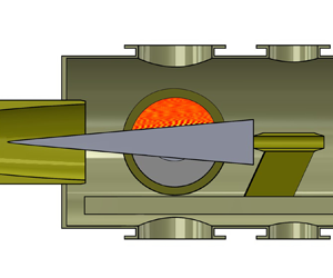
Experiments in this study were conducted in the T5 reflected-shock tunnel at Caltech. The facility design and operation are detailed in Hornung (Reference Hornung1992) and Jewell (Reference Jewell2014) and described here briefly. A schematic of T5 is shown in figure 1. Moving in the downstream direction, the tunnel can be segmented into the following components: secondary reservoir; piston; compression tube (CT); primary diaphragm; shock tube (ST); secondary diaphragm; contoured nozzle; test section; dump tank. Before a shot, the test section, dump tank and both tubes are evacuated. Then the ST is filled with ALPHAGAZ air to the desired test-gas pressure  $P_1$, and the CT is filled with an argon–helium mixture to the desired driver pressure $P_{CT}$. Finally the secondary reservoir, upstream of the piston, is filled with compressed air to a specified gage pressure $P_{2R}$, around 1200 psi for these experiments. Once exposed to the pressure in the secondary reservoir, the 120-kg piston travels downstream, adiabatically compressing the driver gas mixture to a desired value $P_4$. At this point the pressure difference between the driver gas in the CT and the test gas in the ST is high enough to burst the primary stainless-steel diaphragm. The generated shock wave travels through the ST at speed $U_s$, compressing the test gas, and then reflects at the downstream end of the ST, bursting the secondary mylar diaphragm. Under tailored operation, the test gas is considered stagnant after being additionally compressed and heated from the shock reflection to an ultimate reservoir pressure $P_R$ and temperature $T_R$. This flow is then accelerated through the axisymmetric nozzle to Mach 5, and hypervelocity flow is established for approximately 1 ms in the test section. For the present study, total enthalpies $h_0$ around $9\ {\rm MJ}\ {\rm kg}^{-1}$ were established for both shots, resulting in wall-to-edge temperature ratios $T_w/T_e$ of $0.18$. Relative to the adiabatic wall temperature $T_{aw}$, this temperature ratio is $T_w/T_{aw} = 0.057$.

Figure 1. Schematic of T5 reflected-shock tunnel.
Table 1 lists the relevant nozzle reservoir and free stream run conditions for the tests analysed below. The thermodynamic state of the test gas in the nozzle reservoir is determined using the test-gas pressure,  $P_1$, and the measured incident shock speed, $U_s$. We use Cantera (Goodwin, Moffat & Speth Reference Goodwin, Moffat and Speth2009) with the Shock and Detonation Toolbox (Browne, Ziegler & Shepherd Reference Browne, Ziegler and Shepherd2008) to determine the reservoir conditions. The free stream conditions at the exit of the nozzle are obtained through a simulation performed using the University of Minnesota Nozzle Code (Wright, Candler & Prampolini Reference Wright, Candler and Prampolini1996; Johnson Reference Johnson2000; Candler Reference Candler2005; Wagnild Reference Wagnild2012). The free stream conditions are chosen to be an areal average of the data-parallel lower-upper relaxation (DPLR) output at approximately $580\pm 10$ mm, which was the estimated distance from the nozzle throat to the location of the cone's nose tip during the experiment. It is important to note that the release of energy for recombination in the nozzle results in the relatively high $T_{\infty }$ compared with $T_0$. Table 1 also lists the uncertainty values associated with the reservoir and free stream conditions, as calculated by Parziale (Reference Parziale2013). The uncertainty in reservoir conditions corresponds to bias uncertainty originating in $P_R$, $U_s$ and $P_1$. The uncertainty in free stream conditions corresponds to that in the reservoir conditions propagated through the nozzle code as well as nozzle spatial inhomogeneity.
Table 1. Flow conditions.

The model was a  $5^{\circ }$-half-angle cone, 99 cm in total length. The frustum section was aluminium and 83 cm in length, and the 16-cm molybdenum nose tip had a nose radius of $R_N = 2$ mm. The model was installed at nominally zero incidence for all the shots. During the experimental set-up, a digital inclinometer was placed on the cone to measure the cone's angle of attack. The inclinometer provided angular deviation with respect to the cone's half-angle ( $5^\circ$) with a resolution of $0.1^\circ$. The deviation was minimized by placing shims underneath the feet of the cone's sting to achieve an angle of attack of $0.0\pm 0.1^{\circ }$.
3. Diagnostic techniques
Schlieren and FLDI were utilized to analyse boundary-layer content. The schlieren set-up explained by Paquin et al. (Reference Paquin, Skinner, Laurence, Hameed, Shekhtman, Parziale, Yu and Austin2022) was employed here. Illumination was generated by a Cavilux HF laser, and an adjustable iris diaphragm was used to limit the amount of light in an effort to avoid saturation. The beam was expanded through a plano–convex lens, collimated by a parabolic mirror, and directed by a few planar mirrors through the test section. A parabolic mirror focused the beam back down to a point, where the knife edge was inserted. Finally, the beam passed through a bandpass filter, which prevented the test-gas luminosity from obscuring the signal, and then a series of long-focal-length plano–convex lenses, which were used to modify the magnification of the images. A Phantom TMX 7510 camera was used to collect images with a  $1280\times 64$-pixel resolution and a $0.15\ {\rm mm}\ {\rm pixel}^{-1}$ spatial scale. Images were collected at a frame rate of 669 kHz with a laser pulse width of 30 ns. Figure 2 depicts the resulting field of view (FOV) along the cone imaged with schlieren. The images captured a $17\times 1$-cm region whose upstream edge was stationed 58 cm downstream of the nose tip.

Figure 2. Location of diagnostics on cone. The 17-cm-long schlieren FOV is highlighted in red and the FLDI focus at 68 cm is labelled.
As shown in figure 2, the FLDI beams were positioned at  $x = 680$ mm along the cone surface. To establish the quad-FLDI (Q-FLDI) set-up used in this experimental campaign and also discussed in Hameed et al. (Reference Hameed, Shekhtman, Parziale, Paquin, Skinner, Laurence, Yu and Austin2022), the linearly polarized beam generated by a 532-nm Cobolt 05-01 Samba laser was first expanded using a diverging lens. The expanding beam was then split into one column of six ‘spots’ using a Holo/Or MS-474-Q-Y-A diffractive optic. The position along the beam path and orientation of this diffractive optic set the wall-normal interspacing of the FLDI beams. Another Holo/Or diffractive optic (DS-192-Q-Y-A) was used to make an additional column of the already split beams. This diffractive optic set the streamwise interspacing of the FLDI beams. The two columns and six rows of beams generated by the diffractive optic were sent through a quarter-wave plate before being split once more by a 2-arcminute Wollaston prism to generate the intraspaced beam pairs in the FLDI set-up. The beam pairs were then focused inside of the test section at the centre of the cone using a converging lens of an appropriate focal length. A second Wollaston prism of equal separation angle and a linear polarizer was used to recombine the intraspaced beams. Four of the twelve ‘spots’ generated by the diffractive optics were selected to be directed onto photodetectors (Thorlabs DET36A2). The interference between the intraspaced beam pairs resulted in a change in intensity and was measured as a change in voltage by the photodetector. The beams were oriented such that the streamwise interspacing and intraspacing were parallel to the cone's surface, and the wall-normal interspacing was perpendicular to the cone's surface. For these experiments, the beams were interspaced by 1.03 mm and 1.71 mm in the wall-normal and streamwise directions, respectively, and a streamwise intraspacing of 0.18 mm was achieved. The lower set of beams were positioned at $0.64\pm 0.03$ mm above the cone's surface, within the 1 mm boundary layer that was estimated for these experiments. Given the wall-normal beam interspacing, this placed subsequent rows of beams at approximately 1.7 mm and 2.7 mm above the cone's surface. Measurements on the photodetectors were collected with a sampling rate of 100 MHz and a bandwidth of 25 MHz.
4. Stability calculations
Stability calculations for these experiments were performed using the STABL software package (Johnson, Seipp & Candler Reference Johnson, Seipp and Candler1998; Johnson Reference Johnson2000). The computational grids for the mean flow analysis were generated within STABL. To better capture the flow physics in critical regions, the grids were clustered near the tip of the cone and towards the cone's surface by exponential stretching in the streamwise and wall-normal directions. A minimum surface normal spacing was chosen to maintain a  $y_{wall}^+$ value of less than one along the length of the cone. The grid-tailoring routine within STABL was employed to generate a shock-fitted grid for the blunted cone models. Initially, an intentionally oversized grid was used to ensure the shock was completely captured. Using this grid, the mean flow was analysed with particular attention paid to the area in proximity to the cone's blunt nose tip to ensure the local residual in this region was approximately $1\times 10^{-12}$. The solution was then frozen in this domain and the flow around the rest of the model was resolved. Next, the mean-flow solution generated using the initial grid was postprocessed, and the upper grid definition and body-normal spacing was tailored by STABL to generate a shock-fitted grid. In a process similar to the one used with the initial grid, the mean-flow analysis was rerun using the tailored grid to produce a higher-quality mean-flow solution to input into the stability analysis.
The STABL software package uses a two-dimensional/axisymmetric mean flow solver based on NASA's implicit DPLR method (Wright, Candler & Bose Reference Wright, Candler and Bose1998). The STABL DPLR solver uses an extended set of the Navier–Stokes equations with a two-temperature model to characterize the translational, rotational and vibrational modes. Additional details, including the governing equations used by the mean flow solver, can be found in Johnson & Candler (Reference Johnson and Candler2005) and Johnson (Reference Johnson2000). The boundary-layer thickness based on the mean flow solution was approximately 1 mm.
The stability analysis of the flow was performed using PSE-Chem, the parabolized stability equation (PSE) solver within STABL. The PSE-Chem solver was also used to solve the LST equations, which it does by making the ‘locally parallel’ assumption that the mean flow only varies in the body-normal direction. In LST, perturbations are assumed to be described by the normal mode,
 \begin{equation} q'(x,y,z,t)=\hat{q}(y)\exp({\rm i}(\alpha x+\beta z-\omega t)), \end{equation}
where  $q'$ is a disturbance at a position along the cone with an amplitude $\hat {q}=\hat {q}(y)$, $x$ is the streamwise direction, $y$ is the wall-normal direction and $z$ is the azimuthal direction. The spatial linear stability problem is analysed assuming the angular frequency, $\omega$, is real, the streamwise wavenumber, $\alpha$, is complex ( $\alpha = \alpha _r + \alpha _i$), and the azimuthal wavenumber, $\beta$, is not considered as the disturbance is assumed to be two-dimensional. To begin the LST analysis, a frequency range around the estimated disturbance frequency is selected. The PSE-Chem solver estimates the disturbance frequency range of the second and higher disturbance modes using the characteristic time of wave travel between the wall and the relative sonic line (Johnson & Candler Reference Johnson and Candler2005). Spectra of wavenumber guesses are evaluated using LST, and only the most unstable converged solution at each frequency is retained. The results of the linear stability analysis are then used as initial values for the PSE analysis beginning with the lowest-frequency critical point of the LST disturbance amplification rate curve.
The PSE-Chem solver solves the linear parabolized stability equations derived from the axisymmetric Navier–Stokes equations (Johnson & Candler Reference Johnson and Candler2005). The parabolized stability equations are developed by perturbing the mean flow with a fluctuating component, substituting this set of equations into the Navier–Stokes equations and subtracting the mean flow from the result. The resulting second-order partial differential equations are parabolized and an initial solution is generated by assuming the initial disturbances are small and the flow is ‘locally parallel’ at the starting plane (MacLean et al. Reference MacLean, Mundy, Wadhams, Holden, Johnson and Candler2007). The initial solution is marched downstream by simultaneously updating the complex streamwise wavenumber and the disturbance shape function (Johnson & Candler Reference Johnson and Candler2005). Boundary-layer transition is predicted by PSE-Chem using the semiempirical  $e^N$ correlation method (Johnson & Candler Reference Johnson and Candler2005), where $N$ is the $N$ factor defined by
 \begin{equation} N(\omega,s)= \int_{s_0}^{s} \left[-\alpha_i + \frac{1}{2E} \frac{{\rm d}E}{{\rm d}s} \right]{\rm d}s. \end{equation}
Here, the integration is performed at a constant angular frequency,  $\omega$; $s_0$ is the first neutral point at a given frequency; $-\alpha _i$ is the imaginary part of the complex streamwise wavenumber; $E$ is the disturbance kinetic energy.
The stability analysis was performed using a single, highly concentrated stability grid with frequencies ranging from 850 to 3000 kHz and spanning the extent of the 99-cm-long cone. Figure 3 shows the spatial growth rate,  $-\alpha _i$, and $N$ factor (figure 3a) and the phase speed (figure 3b) as a function of the disturbance frequency for Shot 2988 within the measurement region, $x= 0.660$ m. The phase speed, $c_r$, was obtained directly from STABL as the ratio $c_r = \omega /\alpha _r$, where $\alpha _r$ is the real component of the complex streamwise wavenumber. The most unstable frequency, $f_{\alpha }$, corresponding to the maximum growth rate ( $-\alpha _i$), is 1280 kHz. As shown by the black vertical dashed line spanning figure 3(a) and figure 3(b), and similar to the observations of Bitter & Shepherd (Reference Bitter and Shepherd2015), the growth-rate curve for disturbances in this highly cooled boundary layer exhibits a kink at 1480 kHz. This phenomenon, associated with the supersonic mode instability, occurs when the dimensionless phase speed decreases below $1-1/M_e$ and the unstable modes propagate supersonically with respect to the free stream. Thus, frequencies associated with the supersonic mode instability, $f_{SS}$, start at 1480 kHz and persist over the range $1480 \leq f_{SS} < 1600$ kHz. Just past $f = 1600$ kHz, the phase speed then rises back up, surpassing $1-1/M_e$. The most-amplified frequency, $f_{amp}$, corresponding to the highest value of $N$, is 1450 kHz, which is just 2 % lower than the beginning of the supersonic-mode instability $f_{SS}$ at 1480 kHz. It is also to be noted that $f_{amp}$ is 13 % higher than the most unstable frequency $f_{\alpha } = 1280$ kHz, at the same location along the cone. We expect that the experimental frequencies measured here would fall somewhere between $f_{\alpha }$ and $f_{amp}$, since the disturbances in the tunnel start off with a finite rather than infinitesimal amplitude.

Figure 3. Stability results showing predicted growth rate and  $N$ factor (a) and phase speed (b) of instabilities at $x = 660$ mm. The black, vertical dashed line indicates the onset of supersonic mode instability.
5. Results
5.1. Time-resolved modal content
The present study seeks to extract insight from boundary-layer phenomena which occur during short time intervals. This section shows both averaged and time-resolved spectral content generated from schlieren and FLDI diagnostics. To process schlieren data, the boundary layer height was measured from reference-subtracted images using a Sobel filter as in Paquin, Skinner & Laurence (Reference Paquin, Skinner and Laurence2023b), and the average for Shot 2988 was  $\delta = 0.95\pm 0.04$ mm. Wavelet transforms were utilized to identify wave packets in individual images, as discussed by Shumway & Laurence (Reference Shumway and Laurence2015). Sequential images were then cross-correlated to determine the propagation speed of individual wave packets. Using the standard deviation of speeds as an estimate of uncertainty, the average propagation speed $u_p$ identified for the shot was $3340\pm 150\ {\rm m}\ {\rm s}^{-1}$. Spectral content could then be generated using two different methods: time reconstruction or wavenumber transform. Using the reconstruction method discussed in Kennedy et al. (Reference Kennedy, Laurence, Smith and Marineau2018), spatial pixel intensities were converted to time signals. This allowed frequency content to be assessed directly using discrete Fourier transforms. Using the wavenumber transform method, spatial power spectral density (PSD) estimates were generated directly from each image by taking the discrete Fourier transform of a bin of spatial pixel intensities. This wavenumber PSD could then be scaled by $u_p$ to provide an estimate of the frequency distribution. It is to be noted that this latter method does not account for the effect of dispersion on modal content within the boundary layer but provides an estimate of the overall frequency content. The effect of dispersion will be discussed in the next section.
Figure 4 shows spectral content at different heights above the cone surface from Shot 2988. Figure 4(a) displays the averaged PSD curves generated using the time reconstruction method at three discrete wall normal heights:  $y = 0.15$, 0.74 and 1.19 mm, i.e. $y/\delta = 0.16$, 0.78 and 1.25. To characterize the overall trend in the curves, peak frequencies were determined by first identifying the raw maximum in each curve, then fitting a parabola to the 140 kHz region around the raw maximum, and finally identifying the maximum of the parabola as the peak frequency. As shown, the peak frequency resolved right above the wall is 1270 kHz. Moving away from the wall, the PSD peak drops in power, and the peak frequency shifts to $f = 1250$ kHz at $y = 0.74$ mm. Outside the boundary layer at $y = 1.19$ mm, a modest peak sits at $1230$ kHz. At this height, the power within the second-mode band has dropped significantly but the lower-frequency content is elevated. Figure 4(b) shows the spectrogram, or visualization of time-resolved spectral content, generated using the wavenumber transform method at the same discrete heights. In this case, wavenumber transforms were generated by taking the discrete Fourier transform of a 60-mm, or 403-pixel, bin centred around $x = 670$ mm. By comparing the spectra in figure 4(b), it is noted that the highest signal-to-noise ratio exists right above the wall, $y = 0.15$ mm, as could be expected from the PSD curves in figure 4(a). The passage of a turbulent spot manifests itself as the broadband spike at all heights for $t = 0.23\unicode{x2013}0.28$ ms, but strong peaks at later times can be identified in the 1000–1500 kHz range, corresponding to the signature of the second-mode instability predicted by stability calculations. At $y = 0.15$ mm, bursts of modal content are demarcated by bright spots, for example those centred around $t = 0.53$, 0.63, 0.68 and 0.78 ms. The $y = 0.74$ mm spectrogram shows similar peaks, each enduring for approximately $20\ \mathrm {\mu }{\rm s}$. It is to be noted that, even outside the boundary layer, very short bursts of content appear in the 1000–1500 kHz band, for example, one bright spot at $t = 0.63$ ms and another at $t = 0.68$ ms. Further investigation into these bursts identified in the schlieren data is detailed in § 5.2.

Figure 4. Schlieren-based spectra of modal content at three discrete wall-normal heights. Average frequency content for  $x = 680 \pm 12$ mm generated from the time reconstruction method is shown in (a). The time-resolved spectrogram computed using the wavenumber transform method is shown in (b), where frequency content was calculated by scaling wavenumber transforms by the average propagation speed.
Figure 5 shows the evolution of spectral content in the streamwise direction for three time segments:  $0.5 \leq t \leq 0.6$ ms, $0.6 \leq t \leq 0.7$ ms and $0.75 \leq t \leq 0.85$ ms, all at $y =0.15$ mm. Each of these segments contains at least one burst of second-mode content, as can be seen in the spectrogram of figure 4(b). The PSD estimations at each location $x$ were generated using Welch's method. The 0.1 ms segment length of each burst corresponded to $L_{seg} = 2200$ reconstructed data points. Hamming windows $0.8 L_{seg}$ points in length were utilized with $0.7 L_{seg}$ overlap. The first two segments show a similar trend in PSD power. In figures 5(a) and 5(b), the PSD power rises until $x \approx 650$ mm, drops in power until $x \approx 660$ mm and has one additional modest rise until $x \approx 670$ mm before rapidly falling and spreading in frequency. For the $0.5 \leq t \leq 0.6$ ms burst, the peak frequency remains at $f = 1280$ kHz. For the $0.6 \leq t \leq 0.7$ ms burst, the peak frequency shifts from $f = 1270$ kHz at $x \approx 650$ mm to $f = 1210$ kHz at $x \approx 670$ mm. By $x \approx 680$ mm in figure 5(b), the large singular spectral peak has evolved into three smaller peaks at $f = 1100$, 1180 and 1270 kHz. As will be discussed in § 5.2, these split peaks could indicate dispersion within the wave packet. In figure 5(c), the $0.75 \leq t \leq 0.85$ ms burst has a unique development with less-drastic peaks and more energy in the low-frequency band. A modest 1290 kHz peak saturates at $x \approx 615$ mm, drops, and then rises back up until $x \approx 630$ mm. After this point, the peak appears to modulate, generating a smaller peak near $f = 1000$ kHz, until all peaks decay in power by $x \approx 680$ mm. These spectra, and the mechanisms of energy exchange which cause them to modulate, are discussed more in the following sections.

Figure 5. The PSD of reconstructed pixel signals for  $t = 0.5\unicode{x2013}0.6$ ms (a), $t = 0.6\unicode{x2013}0.7$ ms (b) and $t = 0.75\unicode{x2013}0.85$ ms (c), at various locations along cone, $605 \leq x \leq 690$ mm.
Figure 6 shows an averaged PSD generated from the FLDI data, and figure 7 shows spectrograms generated from each of the four probes throughout Shot 2990. As mentioned, the four FLDI probes were positioned at approximately 680 mm from the blunt nose tip with a 1.7-mm streamwise separation between the ‘upstream’ and the ‘downstream’ probes. The averaged PSD was generated using Welch's method, employing Hann windows with a segmentation length of 2048 samples and a 50 % overlap. Similarly, the spectrograms were generated using MATLAB's built-in spectrogram function using Hann windows of 2048 samples.

Figure 6. Averaged PSD generated from data captured by FLDI probes. The second-mode instability is found to exist within the boundary layer at approximately 1250 kHz. Broadband features outside of the boundary layer elevate the low-frequency content for the probes at  $y = 1.7$ and 2.7 mm.

Figure 7. Spectrograms generated from FLDI probes at  $y = 2.7$ mm (a), $y = 1.7$ mm (b), $y = 0.6$ mm upstream (c) and $y = 0.6$ mm downstream (d).
The average PSD curves of the  $y = 0.6$ mm probes in figure 6 indicate that the dominant second-mode frequency sits at 1250 kHz. The time-resolved spectrograms for these probes in figure 7 shows second-mode bursts occurring intermittently throughout the test time. During these instances of observed second-mode content, there are also broadband streaks with elevated lower-frequency content measured by the FLDI probes outside of the boundary layer. The dominant frequency of the second-mode instability measured by FLDI at $y = 0.6$ mm matches the schlieren-resolved frequency at $y = 0.74$ mm and falls within 1 % of the schlieren-resolved frequency at $y = 0.15$ mm. Relative to stability calculations, the experimental second-mode frequencies diverge significantly from the most-amplified frequency $f_{amp}$ but fall close to the predicted most-unstable frequency $f_{\alpha }$. The schlieren peak right above the wall falls 12 % below $f_{amp}$ and 1 % below $f_{\alpha }$, and the FLDI peak falls 14 % below $f_{amp}$ and 3 % below $f_{\alpha }$. It is to be noted that Parziale et al. (Reference Parziale, Shepherd and Hornung2015) also found that FLDI-measured second-mode frequencies fell systematically below those predicted by LST, speculating that this difference could be due to nonlinear effects and/or uncertainty in flow conditions. They found that the sensitivity of the second-mode frequency to condition uncertainty was estimated to be $df/f = 15\unicode{x2013}20\,\%$. Thus, the discrepancy seen here could similarly be attributed to nonlinear effects and uncertainty in flow properties.
5.2. Wave packet modulation
Analysis of the schlieren images allows insight into the development and modulation of wave packets as they progress through the FOV. In this section, we first contextualize the modulation analysis within the framework of computational studies. Many numerical studies have depicted how various instability modes at low  $T_w/T_e$ would manifest themselves in wave packets. Salemi et al. (Reference Salemi, Fasel, Wernz and Marquart2014) and Salemi & Fasel (Reference Salemi and Fasel2015) explained that, as wave packets develop, they synchronize with fast acoustic waves, then vortical/entropic waves and finally slow acoustic waves. At the point of vortical/entropic synchronization, a secondary lower-frequency peak appears within the second mode band, and the wave packet appears to bifurcate into a leading and trailing section due to dispersion. At the point of slow-acoustic-wave synchronization, the lower-frequency peak dominates, and the wave packet stretches significantly. Salemi & Fasel (Reference Salemi and Fasel2018) and Chuvakhov & Fedorov (Reference Chuvakhov and Fedorov2016) furthered this study, incorporating the acoustic-radiation phenomenon. Salemi & Fasel (Reference Salemi and Fasel2018) showed that, at the point of synchronization with vortical/entropic waves, a central portion of the wave packet extends to the top of the boundary layer. Then, at the slow-acoustic synchronization point, wave components extend out into the free stream, generating the acoustic emission characteristic of the supersonic mode, and stretching the packet along the wall. Chuvakhov & Fedorov (Reference Chuvakhov and Fedorov2016) also associated wave packet elongation with slow-acoustic synchronization, showing also that lower-frequency wave components emit stronger acoustic radiation into the free stream. Bitter & Shepherd (Reference Bitter and Shepherd2015) explained this phenomenon in terms of eigenfunctions. For waves synchronizing with the slow acoustic mode in a highly cooled boundary layer, a second sonic line is introduced above the critical layer, and this sonic line acts as a ‘turning point’ which causes the radiation of acoustic waves.
In § 5.2.1, we investigate wave packet modulation due to the interplay of two discrete frequency disturbances using bandpass filtering. In § 5.2.2, we assess the potential existence of various instability modes using space–time POD.
5.2.1. Bandpass filtering
Three bursts of content within the second-mode band from the spectrogram are investigated in this section:  $0.62 \leq t \leq 0.64$ ms; $0.67 \leq t \leq 0.69$ ms; $0.77 \leq t \leq 0.79$ ms. Figure 8 shows the analysis for $0.62 \leq t \leq 0.64$ ms, where figure 8(a) shows the sequence of reference-subtracted schlieren images from this burst. The wave packet is first visible at $t = 0.618$ ms as a series of light/dark streaks right at the wall at $x \approx 635$ mm. This instability is noticeably distinct from those captured in lower-enthalpy facilities, such as the disturbances discussed by Kennedy (Reference Kennedy2019) at stagnation enthalpies $h_0 \leq 2\ {\rm MJ}\ {\rm kg}^{-1}$, where waves are most prominent at the top of the boundary layer, and maximum spectral energy occurs at $y/\delta \geq 0.8$. As the wave packet progresses, the structures reach higher into the boundary layer. By $t = 0.631$ ms, pointed peaks extend through the edge of the boundary layer, and by $t = 0.635$ ms, the density fluctuations appear to reach a maximum, with the highest level of contrast sitting clearly at $660 \lesssim x \lesssim 680$ mm. After this point, the structure becomes less organized and, by $t = 0.644$ ms, the clear peaks have faded, but smaller, fainter waves can still be seen right along the wall for $655 \lesssim x \lesssim 690$ mm.

Figure 8. Wave packet modulation analysis of burst at  $t = 0.62\unicode{x2013}0.64$ ms. Reference-subtracted schlieren images showing growth and then attenuation of wave packet (a), and bandpass-filtered signal along the wall (b).
To better understand the modulation of modal content during wave packet development, bandpass filtering was applied to the row of pixel intensities right above the wall. Figure 8(b) displays pairs of bandpass-filtered intensity signals  $I_{BP}$ for each schlieren image shown in figure 8(a). The pixel intensities were filtered around wavenumbers corresponding to a low frequency ( $\,f_{low} = 1180$ kHz) and high frequency ( $\,f_{high} = 1370$ kHz) within the second-mode band. Passband frequencies were set to $f_{low} \pm 3\,\%$ and $f_{high} \pm 3\,\%$. A Hilbert transform was used to generate the signal envelopes overlaid on the plot. As shown in figure 8(b), high- and low-frequency content coexist within the wave packet along the wall, with the low-frequency content confined to a smaller region in the trailing edge of the packet at $t = 0.627$ ms. In the next instance $t = 0.631$ ms, the low-frequency content moves towards the leading edge of the packet and exceeds the $f_{high}$ intensity in power. For $t = 0.640\unicode{x2013}0.644$ ms, $I_{BP}$ has lowered for both frequencies, but the $f_{low}$ intensity leads the wave packet while the high-frequency content spreads over a larger area. At $t = 0.644$ ms, the $f_{high}$ intensity appears to reach as far upstream as $x \approx 630$ mm, which could indicate that the disturbance is synchronizing with slow acoustic waves and elongating, as predicted by the aforementioned numerical studies (Salemi et al. Reference Salemi, Fasel, Wernz and Marquart2014; Salemi & Fasel Reference Salemi and Fasel2015, Reference Salemi and Fasel2018; Chuvakhov & Fedorov Reference Chuvakhov and Fedorov2016). It is to be noted that this could also correspond to a new wave packet propagating into the FOV. The flow phenomena occurring in this instance are discussed further in § 5.2.2.
Figure 9 shows the analysis for the second burst at  $0.67 \leq t \leq 0.69$ ms, with figure 9(a) showing the sequence of reference-subtracted schlieren images and figure 9(b) showing the bandpass-filtered signals $I_{BP}$ for each frame. Similar to the first burst at $t = 0.62\unicode{x2013}0.65$ ms, one wave packet begins just in the thin layer along the wall near $x \approx 630$ mm at $t = 0.665$ ms. Figure 9(a) shows that, as this disturbance progresses, the waves extend up to the boundary-layer edge. Figure 9(b) shows that the largest variations in $I_{BP}$ can be associated with this primary wave packet, which propagates to 690 mm by $t = 0.688$ ms. Both $f_{low}$ and $f_{high}$ intensity grow in strength over the first few frames, with the $f_{low}$ content pushing towards the leading edge of the wave packet. By $t = 0.688$ ms, $I_{BP}$ of both frequencies decreases within the primary wave packet.

Figure 9. Wave packet modulation analysis of burst at  $t = 0.67\unicode{x2013}0.69$ ms. Reference-subtracted schlieren images showing wave packet progression and emission of a bright spot (a), and bandpass-filtered signal along the wall (b).
Unique from the first burst, however, this sequence demonstrates the simultaneous progression of various wave-like segments. For example, small waves distinct from the primary wave packet sit near  $670 \lesssim x \lesssim 680$ mm for $t = 0.665\unicode{x2013}0.674$ ms, as can be seen in figure 9(b). At $t = 0.674$ ms, the high-frequency envelope of this downstream structure is visible over $667 \lesssim x \lesssim 685$ mm, but by $t = 0.679$ ms, this envelope is largely swallowed into the primary packet, which again suggests dispersion between the low- and high-frequency wave components. Another larger wave structure enters the frame upstream of the primary wave packet at $t = 0.674$ ms, dominated by $f_{low}$ content. By $t = 0.692$ ms, the intensity of all wave packets along the wall has diminished; however, it is important to note that the modal content within the upstream disturbance has simply moved higher in the boundary layer and thus is not apparent in the $I_{BP}$ curve plotted here. This instability eventually transitions into a turbulent spot downstream past $x = 700$ mm. Also unique to this burst, a radiative structure emanates from the primary wave packet, generating a bright spot outside the boundary layer for $t = 0.679\unicode{x2013}0.692$ ms. In light of the predicted acoustic radiation due to the supersonic-mode instability, this phenomenon is further investigated later in this paper. We note that Chuvakhov & Fedorov (Reference Chuvakhov and Fedorov2016) have identified this radiation as a mechanism of energy transfer which limits the growth of the disturbance in the boundary layer. Thus, acoustic radiation could be one cause of the drop in $I_{BP}$ for $t = 0.688\unicode{x2013}0.692$ ms.
Finally, figure 10 shows the modulation analysis for the third burst of content, with figure 10(a) displaying the series of reference-subtracted schlieren images at  $t = 0.77\unicode{x2013}0.79$ ms. Figure 10(b) displays the bandpass-filtered signals, where the passband frequencies, $f_{low} = 1200$ kHz and $f_{high} = 1390$ kHz, were adjusted since this disturbance was at a slightly higher frequency. In the first frame of figure 10(a) at $t = 0.766$ ms, a wave packet can be identified in the boundary layer at $595 \lesssim x \lesssim 630$ mm. In figure 10(b), the $f_{high}$ and $f_{low}$ envelopes largely overlap for this first time step. Progressing in time, the wave packet propagates downstream and elongates, stretching over $610 \lesssim x \lesssim 655$ mm at $t = 0.775$ ms. An extending structure, annotated in figure 10(a), also emerges in the frame. Simultaneous with this structure, the $I_{BP}$ envelopes become more irregular. At $t = 0.775$ ms, the $f_{high}$ packet has split into two separate envelopes sitting on either side of the central $f_{low}$ packet. At $t = 0.779$ ms, the extending structure can be identified near $x \approx 630$ mm, and the amplitude of $I_{BP}$ for both $f_{high}$ and $f_{low}$ has decreased in this area. Between $0.779 \leq t \leq 0.788$ ms, the boundary-layer waves become less evident in the schlieren, confined near $x \approx 680$ mm at $t = 0.788$ ms. By the final frame at $t = 0.792$ ms, no waves are evident and no envelopes are visible in the $I_{BP}$ plot. We speculate that the behaviour here could be due to a number of causes. Chuvakhov & Fedorov (Reference Chuvakhov and Fedorov2016) showed that spontaneous radiation due to the supersonic mode can elongate disturbances and also cause them to develop a beating, or modular, structure. Thus, acoustic radiation could be the cause of the extending structure seen emanating out of the boundary layer, the elongation occurring over the first three frames, the splitting of the $f_{high}$ content and the final attenuation of the $I_{BP}$ amplitude. Nonlinear interactions, discussed in the next section, have also been associated with irregular wave packet envelopes. Sivasubramanian & Fasel (Reference Sivasubramanian and Fasel2014) showed that nonlinear effects cause wave packets to develop a ‘dimple’ in their centre, splitting the envelope into two regions. Laurence et al. (Reference Laurence, Wagner and Hannemann2016) experimentally demonstrated a similar kink in the development of a wave packet in a high-enthalpy boundary layer and attributed it to nonlinear effects. Unnikrishnan & Gaitonde (Reference Unnikrishnan and Gaitonde2021) showed that wave packets in highly cooled boundary layers become increasingly nonlinear as they elongate, unlike warmer-wall cases where packets split into a clear nonlinear head and a separate, linear trailing region. Thus, the observations made for this burst of content could be attributed to acoustic radiation, nonlinear interactions or a combination of the two.

Figure 10. Wave packet modulation analysis of burst at  $t = 0.77\unicode{x2013}0.79$ ms. Reference-subtracted schlieren images showing wave packet movement and extending structure (a), and bandpass-filtered signal along the wall (b).
5.2.2. Space–time proper orthogonal decomposition
Proper orthogonal decomposition (POD) has been used widely in studies which seek to disentangle coherent structures from a complex flow field (Aubry et al. Reference Aubry, Holmes, Lumley and Stone1988; Rowley, Colonius & Murray Reference Rowley, Colonius and Murray2004; Peng, Wang & Liu Reference Peng, Wang and Liu2016) or remove noise from a dataset (Brindise & Vlachos Reference Brindise and Vlachos2017; Mendez et al. Reference Mendez, Raiola, Masullo, Discetti, Ianiro, Theunissen and Buchlin2017). Space-only POD, or ‘snapshot’ POD as introduced by Sirovich (Reference Sirovich1987), has been utilized widely to characterize structures in statistically stationary datasets while space–time POD, originally introduced by Lumley (Reference Lumley1970), extracts spatially and temporally evolving structures in transient events (Schmidt & Schmid Reference Schmidt and Schmid2019; Stahl et al. Reference Stahl, Prasad, Goparaju and Gaitonde2023). Space–time POD has also been extended to relate structures to frequency content through spectral POD (SPOD) (Towne, Schmidt & Colonius Reference Towne, Schmidt and Colonius2018). Insofar as SPOD demands large datasets of statistically stationary flows, it is not suitable for the present study. The efficacy of space–time POD has been demonstrated for sparse, intermittent events such as radiative acoustic bursts from a turbulent jet (Schmidt & Schmid Reference Schmidt and Schmid2019) and coherent structures in an incompressible turbulent boundary layer (Borra & Saxton-Fox Reference Borra and Saxton-Fox2021). In this section, we investigate the evolution of modal structures identified through both POD and space–time POD.
Space-only POD was applied to reference-subtracted schlieren images to assess the possibility of extracting coherent structures directly from images. The authors note that Mendez et al. (Reference Mendez, Raiola, Masullo, Discetti, Ianiro, Theunissen and Buchlin2017) filtered out background noise from particle image velocimetry images and reconstructed ideal images using space-only POD modes associated with particle signal. Following this idea, for the present image set, discrete modes associated with wave-like structures in the boundary layer were identified to create a synthesized image of the disturbance. Figure 11 shows an energy-weighted combination of eight POD modes computed for the set of 71 images collected over  $t = 0.6\unicode{x2013}0.7$ ms. The authors note the striking similarity between this reconstructed result and the snapshot at $t = 0.683$ ms in figure 9(a), where periodic structures extend above the boundary layer. For $670 \lesssim x \lesssim 690$ mm, bright structures continuous with the waves below $y = 1$ mm extend out into the free stream, leaning downstream. These structures could be associated with the supersonic-mode radiation which arises at the point of synchronization with slow acoustic waves, as discussed earlier.

Figure 11. Direct schlieren POD of timespan  $t = 0.6\unicode{x2013}0.7$ ms (71 images). Contour represents the energy-weighted combination of eight discrete POD modes.
Space–time POD was applied to reconstructed pixel time signals, i.e. those used to generate the PSD curves in figure 5. To interrogate the evolution of the two individual events, a stacked snapshot matrix was assembled such as discussed in previous literature (Schmidt & Schmid Reference Schmidt and Schmid2019; Borra & Saxton-Fox Reference Borra and Saxton-Fox2021). The stacked snapshot matrix  $\boldsymbol{\mathsf{P}}$ was defined as
 \begin{equation} \boldsymbol{\mathsf{P}} = \begin{bmatrix} p(t_0^{(1)}-t^-) & p(t_0^{(2)}-t^-) & \cdots & p(t_0^{(N)}-t^-) \\ \vdots & \vdots & \ddots & \vdots \\ p(t_0^{(1)}) & p(t_0^{(2)}) & \cdots & p(t_0^{(N)}) \\ \vdots & \vdots & \ddots & \vdots \\ p(t_0^{(1)}+t^+) & p(t_0^{(2)}+t^+) & \cdots & p(t_0^{(N)}+t^+) \end{bmatrix}, \end{equation}
where  $p(t_0^{(N)})$ is the reconstructed pixel-intensity snapshot, $N$ is the number of realizations during each event and $t_0$ is the central time step of each realization. Each realization spanned $M$ time steps including the one at $t_0$. For this study, $N = 3$ realizations were used for each event, and each realization spanned $M = 673$ reconstructed snapshots, such that $\Delta t = t^+ - t^- = 30\ \mathrm {\mu }{\rm s}$ of data. A singular value decomposition was then used to decompose ${{\boldsymbol{\mathsf{P}}}}$ into modes coherent in space and time. Discrete Fourier transforms were then applied to the resulting matrix of time coefficients to relate the POD modes to frequency content. Welch's method was employed using Hamming windows of $0.9 M$ points in length with $0.8 M$ points of overlap. Modes associated with distinct frequency peaks in the second-mode band were then visualized at each of the $N$ realizations.
Figure 12 shows the space–time POD analysis of the first burst identified near  $t = 0.63$ ms in figure 4(b). As shown in figure 12(a), modes corresponding to $f = 1200$ kHz and 1270 kHz were associated with the wave packet seen passing in figure 8(a). In the first realization centred at $t = 0.625$ ms in figure 12(b), the 1200 kHz mode manifests itself strongly around $655 \lesssim x \lesssim 670$ mm, with the portion at $x \approx 660$ mm rising above the boundary layer with near-vertical contours. The higher-frequency mode corresponding to $f = 1270$ kHz is confined close to the wall, leans downstream and extends over $625 \lesssim x \lesssim 655$ mm. At the next realization, the intensity of the 1200 kHz mode has faded, and the disturbance appears more confined to the wall, leaning downstream. At the final realization, $t = 0.645$ ms, the 1270 kHz disturbance intensifies, with the 1270 kHz waves between $670 \lesssim x \lesssim 680$ rising higher than the 1200 kHz waves in the boundary layer.

Figure 12. Space–time POD data from  $t = 0.625\unicode{x2013}0.645$ ms segment of reconstructed schlieren signals: (a) PSD corresponding to two selected mode shapes; (b) mode shapes at $t = 0.625$, 0.635 and 0.645 ms.
Figure 13 shows the space–time POD result from the second event identified near  $t = 0.68$ ms in figure 4(b). As shown in figure 13(a), two discrete modes were identified corresponding to the second mode, at $f = 1200$ kHz and $f = 1290$ kHz. In the first realization at $t = 0.67$ ms, the modes coexist near $x \approx 660$ mm; however, there appears to be some spuriously resolved content near the top of the frame. In the next realization, 1200 kHz disturbances can be identified near $x \approx 630$ mm and $x \approx 675$ mm. Similar to the space-only POD result in figure 11, bright streaks continuous with the wave structure within $670 \lesssim x \lesssim 680$ mm extend out of the boundary layer. Distinct orientation changes can be identified within the disturbance as well. Within the boundary layer, the disturbance creates a ‘<’ shape, but then, for $y > 1$ mm, the disturbance is oriented near vertical, similar to the previous wave packet. A possible explanation for this orientation change is a second sonic line introduced by the supersonic mode, as discussed by Bitter & Shepherd (Reference Bitter and Shepherd2015). In summary, these schlieren and POD sequences exhibit unique events where disturbances extend out of the boundary layer. Although the frequencies associated with the radiating structures are lower than the simulation-predicted $f_{SS}$, they are close to the identified peak second-mode frequency for this burst, 1210 kHz. We speculate that the same systematic divergence between simulated and measured peak second-mode frequency causes the discrepancy between simulated $f_{SS}$ and the frequency associated with the radiating space–time POD modes. It is not clear, however, why the extending structure is more evident in the lower-frequency (1200 kHz) mode rather than the higher-frequency (1290 kHz) mode since the lower end of $f_{SS}$ is predicted to be higher than both $f_{\alpha }$ and $f_{amp}$.

Figure 13. Space–time POD data from  $t = 0.67\unicode{x2013}0.69$ ms segment of reconstructed schlieren signals: (a) PSD corresponding to two selected mode shapes; (b) mode shapes at $t = 0.67$, 0.68 and 0.69 ms.
5.3. Cross-bicoherence
In addition to the growth of wave packets, nonlinear interactions play an important role insofar as they elucidate the energy exchanges leading to breakdown. From a design perspective, they not only determine the onset of turbulent structures but also control the three-dimensional layout of hot streaks on a vehicle (see Sivasubramanian & Fasel Reference Sivasubramanian and Fasel2015; Hader & Fasel Reference Hader and Fasel2019; Hader, Leinemann & Fasel Reference Hader, Leinemann and Fasel2020). To date, aside from the authors’ own work (see Hameed et al. Reference Hameed, Parziale, Paquin, Laurence, Yu and Austin2023; Paquin et al. Reference Paquin, Laurence, Hameed, Parziale, Yu and Austin2023a), very few experimental studies have investigated nonlinear breakdown at flight-relevant enthalpies. In this section, we assess the extent of nonlinear interaction associated with boundary-layer phenomena using cross-bicoherence. Bicoherence is a way of deducing the level of phase locking within a triad of frequencies  $\langle\, f_1, f_2, f_3 = f_1 + f_2 \rangle$. As a result, levels of high bicoherence indicate energy exchange between various modes present within a signal, and the analysis is instrumental in characterizing the nonlinear development of instabilities. Specifically, calculation of the cross-bicoherence between two spatially separated signals, as performed by Ide et al. (Reference Ide, Ito and Tanno2020), allows the identification of sum and difference interactions within a finite region.
Similar to the PSD, which is the Fourier transform of the second-order moment, or autocorrelation function  $R_{qq}$, the bispectrum is the Fourier transform of the third-order moment $R_{qqq}$. This moment is defined as
 \begin{equation} R_{qqq}(\tau_1,\tau_2) = E[q(t)q(t+\tau_1)q(t+\tau_2)], \end{equation}
where  $E$[-] is the expectation operator and $\tau _1$ and $\tau _2$ are time delays. In Fourier space, the bispectrum is then defined as
 \begin{equation} B(f_1,f_2) = E[Q(f_1)Q(f_2)Q^*(f_1+f_2)], \end{equation}
where  $Q(f)$ is the Fourier transform of signal $q(t)$ and $Q^*(f)$ is the complex conjugate. Bicoherence is defined as the normalized bispectrum. In this work, the normalization established by Brillinger (Reference Brillinger1965) was used. Following the notation of Hinich & Wolinsky (Reference Hinich and Wolinsky2005) and Butler & Laurence (Reference Butler and Laurence2021), the bicoherence $b$ is defined as
 \begin{equation} b^2(f_1,f_2) = \frac{|B(f_1,f_2)|^2 }{S(f_1)S(f_2)S(f_1 + f_2)}. \end{equation}
In this normalization, where  $S(f)$ is the PSD power, the magnitude of $b(f_1,f_2)$ is equivalent to a skewness function and not artificially bounded between 0 and 1 (Hinich & Wolinsky Reference Hinich and Wolinsky2005). This technique was used to explore both the schlieren data of Shot 2988 and the FLDI data from Shot 2990. The cross-bicoherence maps for both datasets were generated using the bicoherx function, which is a part of the Higher-Order Spectral Analysis (HOSA) Toolbox in MATLAB.
With the schlieren data from Shot 2988, cross-bicoherence was analysed for the three discrete time segments whose streamwise PSD curves were plotted in figure 5:  $0.5 \leq t \leq 0.6$ ms, $0.6 \leq t \leq 0.7$ ms and $0.75 \leq t \leq 0.85$ ms. The cross-bispectrum was computed for pairs of two reconstructed pixel time signals, $q_x(t)$ and $q_{x+\Delta x}(t)$ spaced $\Delta x = 10$ pixels, or 1.5 mm, apart at various locations along the cone. As mentioned, the 0.1 ms segment corresponded to $L_{seg} = 2200$ reconstructed points in time. Hanning windows were applied to segments 248 points in length with 50 % overlap. Figures 14–16 each show four realizations of cross-bicoherence $b$ at various streamwise locations, along with the associated average PSD calculated for each signal pair. It is to be noted that the streamwise locations are not evenly spaced; the $x$ locations were chosen to highlight unique interactions. All three bursts showed evidence of nonlinear interactions as far upstream as $x \approx 620$ mm, but the highest levels of bicoherence were generally experienced in the region $635 \lesssim x \lesssim 690$ mm, so this is the region analysed here. The PSD curves were computed using the same windowing scheme discussed in § 5.1. In all cases, signals right above the wall ( $\kern 0.06em y = 0.15$ mm) were used for analysis since the highest signal-to-noise ratio was identified here. The axes on the cross-bicoherence maps are normalized by the corresponding second-mode peak frequency $f_{2M}$, which was identified at each location. The corresponding PSD curves show the same frequency domain but in kilohertz. All contours are plotted with the same intensity scale, and the symmetry lines $f_2 = f_1$ and $f_2 = -f_1$ are outlined on each map. It is to be noted that, when describing the frequency triads in $\langle$ $\rangle$ format, we normalize by $f_{2M}$ for simplicity, such that $\langle 1, 1, 2 \rangle$ corresponds to $\langle\, f_{2M}$, $f_{2M}$, 2 $f_{2M}\rangle$. Similarly, the variables $f_1^*$ and $f_2^*$ represent $f_1^* = f_1/f_{2M}$ and $f_2^* = f_2/f_{2M}$.

Figure 14. Schlieren-based cross-bicoherence for Shot 2988,  $0.5 \leq t \leq 0.6$ ms at various streamwise positions: (a) $x = 645$ mm; (b) $x = 651$ mm; (c) $x = 669$ mm; (d) $x = 687$ mm.

Figure 15. Schlieren-based cross-bicoherence for Shot 2988,  $0.6 \leq t \leq 0.7$ ms at various streamwise positions: (a) $x = 650$ mm; (b) $x = 660$ mm; (c) $x = 671$ mm; (d) $x = 683$ mm.

Figure 16. Schlieren-based cross-bicoherence for Shot 2988,  $0.75 \leq t \leq 0.85$ ms at various streamwise positions: (a) $x = 635$ mm; (b) $x = 654$ mm; (c) $x = 671$ mm; (d) $x = 683$ mm.
Figure 14 shows the cross-bicoherence for  $0.5 \leq t \leq 0.6$ ms. Of the three schlieren bursts, this segment showed the overall lowest intensity in bicoherence. At $x = 645$ mm in figure 14(a), the fundamental interacts with low-frequency disturbances in the triad $\langle 1,\approx 0,1\rangle$ as well as the first harmonic in the sum triad $\langle 1,1,2\rangle$ and difference triad $\langle 2,-1,1\rangle$. It is to be noted that subharmonic and first-harmonic disturbances appear in the cross-bicoherence but are not visible in the PSD above the noise floor. By $x = 651$ mm, the primary nonlinear interactions involve lower frequencies and the subharmonic, located in the regions $(0.4 \leq f_1^* \leq 0.6, -0.6 \leq f_2^* \leq -0.4)$ and $(0.3 \leq f_1^* \leq 0.7, -0.2 \leq f_2^* \leq 0.2)$, and the second-mode peak rises in the PSD. In figure 14(c), the highest level of $b$ is experienced at the fundamental–first-harmonic difference interaction $\langle 2,-1,1\rangle$, and the power of the $f_{2M}$ peak reaches its maximum in the PSD. After this point, the peak power decreases and $f_{2M}$ skews towards lower frequencies, indicating wave packet breakdown. The fundamental–low-frequency interactions re-emerge and, along with the fundamental–first-harmonic sum and difference interactions, assist in distributing energy away from the second-mode peak. Figure 14(d) shows the fundamental–low-frequency triads $\langle 1,\approx 0,1\rangle$ and $\langle 1,-1,\approx 0\rangle$, as well as the fundamental–first-harmonic triads $\langle 1,1,2\rangle$ and $\langle 2,-1,1\rangle$.
Figure 15 shows the cross-bicoherence for  $0.6 \leq t \leq 0.7$ ms. At $x = 650$ mm in figure 15(a), some low-frequency interactions are visible in the region $(0.1 \leq f_1^* \leq 0.3, -0.2 \leq f_2^* \leq 0.2)$, but the most significant phase locking exists between the second-mode fundamental and its first harmonic, specifically the sum $\langle 1,1,2\rangle$ and difference $\langle 2,-1,1\rangle$ interactions. At $x = 660$ mm in figure 15(b), interactions involving the first harmonic have faded, and now the maxima in $b$ correspond to phase locking between the fundamental and low-frequency disturbances at $(1 \leq f_1^* \leq 1.2,-0.2 \leq f_2^* \leq 0.2)$ and $(1 \leq f_1^* \leq 1.2,-1.2 \leq f_2^* \leq -1)$. These interactions likely explain the widened base of the second-mode peak in the PSD at $x = 660$ mm. At $x = 671$ mm in figure 15(c), the peak in the PSD has flattened somewhat, and the disturbances begin breakdown. Both fundamental–low-frequency and fundamental–first-harmonic interactions appear, but the highest $b$ corresponds to off-band interactions, for example the difference interactions $\langle 2,-0.8,1.2\rangle$ and $\langle 2,-1.2,0.8\rangle$. The effect of the increased extent of nonlinear interactions is visible in the PSD at $x = 683$ mm, which is located in the triple-peak region identified in figure 5. The modal energy has been redistributed over a larger triple-peaked spectrum, which continues to drop in power moving downstream. The cross-bicoherence map shows that the fundamental–low-frequency interaction re-emerges at $(f_1^* = 1,-0.1 \leq f_2^* \leq 0.1)$. From this point forward, the fundamental–low-frequency and fundamental–first-harmonic triads remain the dominant interactions, as they did for the $0.5 \leq t \leq 0.6$ ms burst.
Finally, figure 16 shows the cross-bicoherence for  $0.75 \leq t \leq 0.85$ ms. This segment demonstrates the largest extent and earliest onset of cross-bicoherence. Unlike the other two bursts, this segment shows no clear rise and saturation of the second-mode peak within the region examined; rather, the locations analysed here fall within the region of modulation and decay discussed in § 5.1. At $x = 635$ mm in figure 16(a), the PSD has two distinct peaks in the second-mode band at 1270 and 1350 kHz. Low-frequency self-interactions $(0 \leq f_1^* \leq 0.5,-0.5 \leq f_2^* \leq 0.5)$ coexist with fundamental–low-frequency interactions near $(0.8 \leq f_1^* \leq 1.2,-0.2 \leq f_2^* \leq 0.2)$ as well as the fundamental–first-harmonic sum interaction $\langle 1,1,2\rangle$ and difference interaction $\langle 2,-1,1\rangle$. At $x = 654$ mm, the second-mode peaks have merged and flattened somewhat, and all nonlinear interactions involving the fundamental have intensified. At $x = 671$ mm, a secondary peak at $f = 1000$ kHz emerges from the second-mode band, and additional lobes appear in the bicoherence contour. The locus of fundamental–low-frequency interactions has split into two triads: $\langle 0.9,0.2,1.1\rangle$ and $\langle 1.1,-0.2,0.9\rangle$. Similarly, the fundamental–first-harmonic interaction has split into $\langle 1.8,-0.9,0.9\rangle$ and $\langle 2.1,-1.1,1.0\rangle$. In the final contour, the nonlinear interactions have weakened and the PSD shows more energy distributed away from the second-mode band. Overall, the cross-bicoherence analysis from bursts of schlieren data indicates that nonlinear interactions accompany the full progression of wave packet development: growth; saturation; breakdown. Interactions between the second-mode fundamental and the first harmonic were generally the most dominant and long-lived. Fundamental–low-frequency interactions also appeared, typically following points of second-mode peak saturation in the PSD. For the $0.6 \leq t \leq 0.7$ ms and $0.75 \leq t \leq 0.85$ ms bursts, cross-bicoherence maps showed that fundamental–first-harmonic and fundamental–low-frequency interactions split into lobes during breakdown, suggesting the mechanism by which secondary peaks were generated in the PSD.
Figure 17 shows the FLDI-based cross-bicoherence computed between the probes within the boundary layer at  $x = 680$ mm for the time duration $t= 2335\ \mathrm {\mu }{\rm s}$ to $t= 2380\ \mathrm {\mu }{\rm s}$. For this dataset, Hanning windows were applied to segments 512 points in length with 50 % overlap. The cross-bicoherence map was limited to show peaks with $b\geq 0.3$ at contour intervals of 0.1. During this short time interval, the second-mode instability was observed by the probes within the boundary layer and a broadband burst was observed by both probes outside of the boundary layer. Similar to the result from schlieren data at $x = 650$ mm for Shot 2988, a strong sum interaction is observed at $\langle 1, 1, 2 \rangle$. This interaction is the nonlinear mechanism by which the first harmonic of the second mode is generated, and is the likely cause of the peak observed in the averaged PSDs for FLDI probes at approximately 2600 kHz. Another weaker sum interaction at $\langle 2, 1, 3 \rangle$ identifies the nonlinear mechanism through which the second harmonic of the second mode is generated. Referring to figure 6, there is no discernible peak observed in the averaged PSD at $3f_{2M}$, suggesting the peak in the cross-bicoherence at this frequency pair represents an early coupling between the second mode and its first harmonic, which contributes to the generation of the second harmonic of the second mode (Craig et al. Reference Craig, Humble, Hofferth and Saric2019). The strong difference interaction at $\langle 2, -1, 1 \rangle$ identifies the mechanism of energy exchange between the second mode and its first harmonic within the boundary layer. Schlieren results indicated that this difference interaction was the strongest interaction at $x = 650$ mm, and it also existed for $671 \leq x \leq 687$ mm. Thus, the wave packets analysed with schlieren and FLDI demonstrated similar nonlinear interactions, which gives confidence that these interactions are representative of the energy exchanges occurring under these flow conditions. It is also to be noted that the schlieren results indicated that nonlinear interactions existed as far upstream as $x = 631$ mm. These interactions could contribute to the discrepancy between stability simulations and measured frequency content since the PSE does not account for nonlinear effects.

Figure 17. The FLDI-based cross-bicoherence calculated between the two probes in the boundary layer at  $x = 680$ mm, $y = 0.6$ mm.
6. Conclusion
Wave packet development was studied by analysing discrete bursts of content from schlieren imaging and FLDI. Stability results indicated that both the second-mode and the supersonic-mode instability would be present, with the beginning of the supersonic-mode band being just 2 % higher than the most-amplified second-mode frequency. Analysis of schlieren-based reconstructed signals showed that strong spectral peaks in the second-mode band persist until  $x \gtrsim 680$ mm on the cone. Bandpass filtering showed evidence of wave packet elongation as well as dispersion between low- and high-frequency disturbances within a wave packet, both of which have been predicted to correspond to slow-acoustic synchronization. Modal reconstruction techniques (space-only POD and space–time POD) indicated the presence of modal content outside the boundary layer, which has been predicted to be the signature of the supersonic-mode instability. Both schlieren and FLDI data were used to compute cross-bicoherence. The most important interactions were found to be between the fundamental (second-mode) frequency and the first harmonic as well as the fundamental and low frequencies. Nonlinear interactions spread into multiple lobes for wave packets that decomposed into split peaks during breakdown.
Overall, this study is the first of its kind to directly address phenomena predicted numerically but never seen experimentally: radiation of structures connected to waves in the boundary layer; dispersion and elongation associated with slow-acoustic synchronization; orientation changes likely due to the supersonic-mode addition of a sonic line. Schlieren and FLDI data showed extremely good agreement in spectral and bispectral measurements, agreeing within 1 % on the peak second-mode frequency at  $x = 680$ mm, and showing the dominance of fundamental–first-harmonic and fundamental–low-frequency interactions at $x = 680$ mm. While this work showed potential evidence of the supersonic mode, it was limited in a few ways. First, the space–time POD-derived frequency of modal content extending out of the boundary layer was lower than predicted for the supersonic mode. More thorough characterization of these extending structures would be needed to confirm the presence of spontaneous acoustic radiation. Future work should involve capturing images at a higher frame rate such that the dataset could resolve more instances of wave packets propagating. This would allow better verification of the POD results as well as more variation in the space–time POD parameters. Second, it was not possible to disentangle the effects of nonlinear interactions from the potential effects of the supersonic mode on the bandpass-filtered signals. Evaluation of wave packet development over a larger area, or farther upstream, may allow clearer discernment of whether or not the supersonic mode is the cause of modal modulation.
Funding
This work was supported by AFOSR grant FA9550-18-1-0403, under program manager Sarah Popkin.
Declaration of interests
The authors report no conflict of interest.


 Open access