


1. Introduction
Swimming mechanisms of marine animals can be categorized generally into lift-based, drag-based and jetting forms of propulsion, based on how thrust is generated (Vogel Reference Vogel2003). While lift-based propulsion by undulating motion is commonly adopted for high-performance swimming or by more aquatically adapted animals (Fish Reference Fish1996), drag-based propulsion has been adopted by many aquatic animals because of its better performance in low-speed swimming and in manoeuvring (Walker & Westneat Reference Walker and Westneat2000). Studies of the mechanism of drag-based propulsion have covered a broad range of topics, including, for example, three-dimensional kinematics of pectoral fins and their relation to the movement of a swimming fish (Lauder & Jayne Reference Lauder and Jayne1996), dynamic modelling of swimming gaits and evaluation of their performance (Walker & Westneat Reference Walker and Westneat2000) combined with actual measurements of fin motion (Walker & Westneat Reference Walker and Westneat2002), three-dimensional vortex formation coupled with thrust generation considering different propulsor geometries (Kim & Gharib Reference Kim and Gharib2011a) and flexibility effects (Kim & Gharib Reference Kim and Gharib2011b), and application of a passive hinge design for the orientation control of pectoral fins of a fish robot (Behbahani & Tan Reference Behbahani and Tan2016). As a fundamental strategy of drag-based propulsion, enhancement of net thrust over a cycle is achieved by modulating the effective area of the propulsor during both power and recovery strokes (Walker Reference Walker2002).
In the context of bio-inspired engineering design, the unique configuration of the arms of crinoids (also known as feather stars) possesses great potential as a propulsor structure that incorporates a significant change in area between power and recovery strokes. The arms of crinoids are feather-like, with lateral extensions known as pinnules that resemble the barbs of a feather. During the recovery stroke, reconfiguring of the arm and its pinnules leads to a dramatic decrease in the area of the arm. Although the swimming performance of actual crinoids has been evaluated using simple biomechanical models (Janevski & Baumiller Reference Janevski and Baumiller2010), the form and function of their unique arms still remain unclear from the perspective of thrust generation.
On the other hand, the reconfiguration represented by passive adaptation of an elastic structure to surrounding flow was first investigated in the context of drag reduction in vegetation, including the pioneering studies by Vogel (Reference Vogel1984, Reference Vogel1989) that introduced the well-known Vogel exponent. Subsequent studies of reconfiguration have characterized successfully the dynamics of elastic structures coupled with steady flow for various geometries and flexibilities, ranging from elastic fibres (Alben, Shelley & Zhang Reference Alben, Shelley and Zhang2002; Gosselin & de Langre Reference Gosselin and de Langre2011) or plates (Gosselin, de Langre & Machado-Almeida Reference Gosselin, de Langre and Machado-Almeida2010; Luhar & Nepf Reference Luhar and Nepf2011; Leclercq & de Langre Reference Leclercq and de Langre2016; Pezzulla et al. Reference Pezzulla, Strong, Gallaire and Reis2020) to various plants (Whittaker et al. Reference Whittaker, Wilson, Aberle, Rauch and Xavier2013; Whittaker, Wilson & Aberle Reference Whittaker, Wilson and Aberle2015). Furthermore, the transient dynamics of elastic structures coupled with unsteady flow conditions has been examined in work by Luhar & Nepf (Reference Luhar and Nepf2016), Leclercq & de Langre (Reference Leclercq and de Langre2018) and Zhang & Nepf (Reference Zhang and Nepf2021). In these studies, for both steady and unsteady flow conditions, the theoretical modelling of the fluid–structure interaction has enabled reasonable estimates to be obtained of the flow-induced forces and resulting deformation of the structures.
In this study, motivated by the unique propulsive feature of a crinoid arm, we investigate experimentally the fluid–structure interaction of a simplified feather-like elastic structure composed of a centre rod to which barb-like rigid side flaps are attached by elastic hinges, aiming to reveal the principles of the complex deformation involving multiple elastic parts (figure 1). For both power and recovery strokes, one end of the centre rod is prescribed to undergo linear translation, resulting in deformation of the centre rod and hinges by interaction with quiescent surrounding fluid. Passive folding of the rigid flaps via the elastic hinges occurs generally in the recovery stroke, which is achieved by allowing the hinges to bend in only one direction. We also establish a theoretical model of the dynamics of the elastic structure. Because the flaps as well as the centre rod undergo reconfiguration in each stroke, the two-dimensional deflections of the centre rod and the flaps need to be coupled in an appropriate manner to fully reconstruct the three-dimensional deformation of the elastic structure. The present study focuses primarily on the quasi-static interaction of the elastic structure with the surrounding flow as a prerequisite to draw general relations between the flow-induced drag and three-dimensional reconfiguration of the structure. Extending the quasi-static analysis, we explore the unsteady dynamics of the elastic structure, although not comprehensively, to identify key differences arising from oscillatory motion.

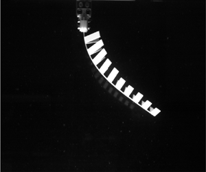
Figure 1. (a) Schematic of the experimental set-up. The initial position of the elastic structure is shown by the dashed line. (b) Schematic of the elastic structure. (c) Illustration of how tape and strips are placed to connect the side flaps to the centre rod. (d) Orientation of (i) the side flaps and (ii) the elastic structure during power and recovery strokes; the arrows in (d) indicate the direction of translation.
Our experimental set-up is described in § 2, and theoretical modelling of the deformation of the elastic structure is conducted in § 3. The characteristics of structural deformation under steady translation are identified, and their dependence on several parameters, such as dimensionless bending stiffness and translational speed, is discussed in § 4.1. In addition, the effects of flap geometry and hinge stiffness on the drag exerted on the elastic structure are examined in § 4.2. The theoretical model is extended to cases with a extremely rigid or flexible centre rod in § 4.3. Finally, the unsteady dynamics of the elastic structure under oscillatory motion is discussed in § 4.4. Our concluding remarks are presented in § 5.
2. Experimental set-up
Experiments were conducted in a water tank with internal dimensions 490 mm width, 1200 mm length and 500 mm height. The elastic structure under consideration was connected to the block of a linear guide (MW-EQB45, NTRexLAB) placed above the water tank (figure 1a). Driven by a stepper motor controlled via a data acquisition board (PCIe-6321, National Instrument Co.), the linear guide block and the clamped top end of the elastic structure underwent translation where a simple code in MATLAB (Mathworks Inc.) was used to prescribe the motion. Both steady and unsteady translational motions of the top end were considered. For the cases of steady motion, translation at a constant speed  $U=U_0$ was prescribed for the power stroke along the positive $x$ axis and for the recovery stroke along the negative $x$ axis, with each stroke being of length 85 cm. For smooth acceleration at the start of each stroke, a quarter of a sinusoidal velocity profile was implemented within the first 10 cm displacement of each stroke. For the cases of unsteady motion, simple oscillation was considered with sinusoidal speed profile $U(t) = U_0 \sin (2{\rm \pi} f t)$ repeated for 10 cycles, where $U_0$ and $f$ are translational speed amplitude and oscillation frequency, respectively. For both steady translation and harmonic oscillation, we waited a couple of minutes between successive cases to settle perturbed flow.
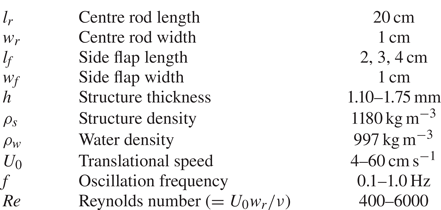
An elastic structure was fabricated with acrylic sheets of thickness  $h = 1.10$–1.75 mm; in this study, the elastic structure comprises the combination of the centre rod and all side flaps. The overall shape of the elastic structure is feather-like, as shown in figure 1(b). Both the centre rod and side flaps were fabricated from a single acrylic sheet to minimize local variations in sheet thickness as much as possible; such local variations were within 5 % of the mean value. The length of the centre rod, $l_{r}$, had fixed value 20 cm, and the length of the side flaps, $l_{f}$, varied from 2 to 4 cm. The widths of the centre rod and side flaps, $w_{r}$ and $w_{f}$, respectively, were 1 cm. A total of 20 side flaps were placed along the longitudinal direction of the centre rod, with 1 cm spacing between adjacent flaps. The Reynolds number $\mbox {{Re}} = U_0 w_{r} /\nu$ was between 400 and 6000, where $U_0$ is the speed amplitude ( $U_0 = 4$–60 cm s $^{-1}$), and $\nu$ is the kinematic viscosity of water ( $\nu = 1.0\times 10^{-6}$ m $^2$ s $^{-1}$ at 20 $^{\circ }$C). The main experimental parameters are summarized in table 1.
Table 1. Experimental parameters.
A high-speed camera (FASTCAM MINI-UX50, Photron, Inc.) with resolution  $1280 \times 1024$ pixels was used to capture the deflected profile of the translating elastic structure in water at 250 f.p.s. for cases with $U_0$ over 30 cm s $^{-1}$, and 125 f.p.s. for the other cases. The image plane was illuminated using an LED lamp. To acquire the deflected profile, raw images were processed using a MATLAB code. A force transducer (MB-5, Interface Inc.) was attached between the linear stage and the model to obtain the drag force acting on the entire model (figure 1a). The transducer was calibrated using various static loads and exhibited repeatable and reliable results with resolution approximately 0.01 N. For a steady translation case, the quasi-steady drag force was acquired at sampling rate 100 Hz by taking the arithmetic mean of the measured values over a certain period of constant translational speed during which the time series data of the force formed a plateau. The time history of the force shows minor variations during steady translation despite highly unsteady wakes behind the elastic structure. The standard deviation of the drag in a plateau is less than 4 % of its mean value for cases with $U_0 > 20$ cm s $^{-1}$, although the standard deviation tends to be relatively larger for low-speed cases with small drag. To eliminate the effect of the submerged part connecting the elastic structure to the linear stage mount, force measurements were also conducted without the elastic structure. By subtracting the force measured in the absence of the elastic structure from the force measured with it present, the drag force of the elastic structure alone could be obtained. Measurements were repeated three times, and the standard deviation was within 5 % of the mean value of the three repetitions for cases with $U_0 > 10$ cm s $^{-1}$. Owing to the limitations on the resolution of the force transducer, the error tended to be amplified for cases with small drag ( $U_0 < 10$ cm s $^{-1}$), where measured drag is comparable to the resolution of the transducer. For an oscillation case, the drag force was acquired at sampling rate 500 Hz over the entire 10 cycles. Similar to the steady translation cases, measurements were also conducted without the elastic structure to eliminate the contribution of the connecting part. As the cyclic motion of the elastic structure was observed after two cycles, the drag force was phase-averaged over the last eight cycles. The root-mean-square error of the phase-averaged data with respect to the raw data was within 6 % of the standard deviation of the raw data over a cycle, indicating good periodicity of the time series data.
The main feature of the elastic structure is the unidirectional bending of the side flaps. The centre rod and side flap were as close as possible to each other, and they were connected using an adhesive tape (3M Scotch Transparent Film Tape 550, 3M) which functioned as an elastic hinge (figure 1c). The tape was attached on only one side of the centre rod and side flap so that the side flap could hinge to the side to which it was taped during the recovery stroke (figure 1d). During the power stroke, the side flaps could not hinge to the other side past the initial flat configuration owing to the restriction on their motion: the side surfaces of the centre rod and the side flaps were in contact with each other because of the finite thickness of the acrylic sheets, thus prohibiting hinge motion. That is, during the power stroke, the side flaps were eventually aligned parallel along the centre rod (figure 1d-i). Because of the asymmetric motion of the side flaps, the deformed shape of the model differed between the two strokes.
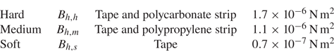
To realize various bending stiffness values of the elastic hinge, a 1 mm wide strip of polycarbonate (PC) or polypropylene (PP) sheet, of thickness 0.2 mm, was placed under the tape (figure 1c); the tape itself was made of 0.038 mm thick PP backing. Thus a total of three types of hinges were tested: only tape, tape with a polycarbonate strip, and tape with a polypropylene strip. These three hinges are hereinafter termed hard, medium and soft, respectively, according to their relative stiffnesses (table 3). The bending stiffness of the hinges will be assessed in § 3.
Even slight variations in the thickness of the acrylic sheet will result in dramatic changes in the bending stiffness of the centre rod,  $B_{r}$. Furthermore, although small, the contributions of the acrylic tape and the elastic strips, providing elastic connections of the multiple side flaps to the centre rod, should be considered. To obtain an accurate measurement of the bending stiffness of the centre rod in its longitudinal direction (along the curvilinear coordinate $s$ in figure 2a), the effective bending stiffness $B_{r}$ was calculated by fitting the actual deflected profile of the elastic structure under gravity, which was obtained from a filmed image, with a theoretically estimated profile based on the nonlinear elastica theory, assuming the centre rod to be a slender body because $l_{r}/w_{r} = 20$ (figure 2); the elastic structure was initially horizontal with its left end clamped. Note that this particular set of experiments was conducted in air rather than water. For the theoretically estimated profile, the following equation was used, which represents a balance between the internal bending force, the gravitational force, and a point load $P$ at the free end:
 \begin{equation} B_{r}\,\frac{\mathrm{d}^2 \theta_{r}(s)}{\mathrm{d}s^2} + \left[\rho_{s} gh \int_{s}^{l_{r}} (w_{r} + 2 l_{sf})\,\mathrm{d}s^* + P\right] \cos \theta_{r}(s) = 0, \end{equation}
where  $l_{sf}$ is a shape function defined to take account of the existence of the side flaps,
 \begin{equation} l_{sf} =\begin{cases} 0 & \textrm{for regions without side flaps}, \\ l_{f} & \textrm{for regions with side flaps}, \end{cases} \end{equation} $\rho _{s}$ is the density of the elastic structure, and $\theta _{r}$ is the deflection angle with respect to the $x$ axis (figure 2a).
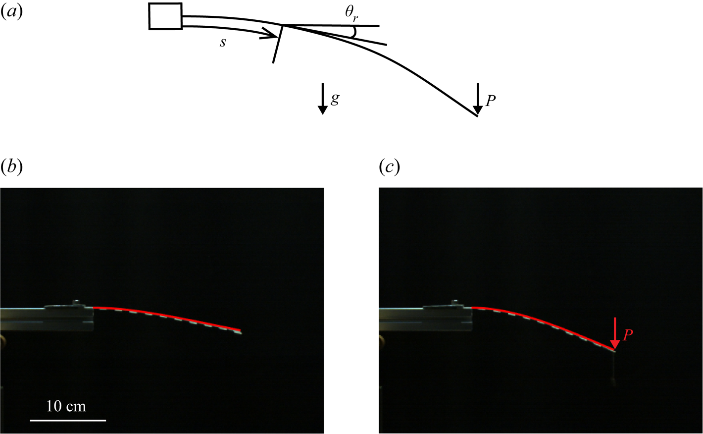
Figure 2. (a) Schematic of the elastic structure under gravity and with a point load  $P$ at the free end. (b,c) Raw images of the bent elastic structure and theoretically estimated profiles (red solid lines) using (2.1): (b) under gravity only; (c) under gravity with the point load at the free end.
To obtain the deflected profile, (2.1) is solved numerically with the following boundary conditions at the clamped and free ends:  $\theta _{r} = 0$ at $s = 0$, and $\mathrm {d}\theta _{r}/\mathrm {d}s = 0$ at $s = l_{r}$. A total of 15 elastic structures with different hinge types and side-flap lengths were tested, both with and without a point load $P$ of 0.23 N for more accurate measurement. The point load was applied at the free end of the elastic structure by attaching a load vertically to the end of the centre rod with a string. The effective bending stiffness
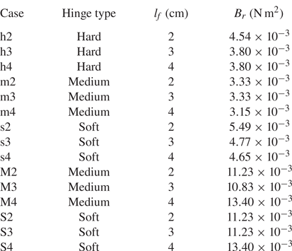
  $B_{r}$ acquired by fitting the actual experimental profile with the theoretical profile from (2.1) is used throughout this study (table 2). The cases in table 2 are divided into those in which the centre rod is thin and those in which it is thick, based on the magnitude of $B_{r}$. In the thin-centre-rod cases, $B_{r}$ ranges from $3.33\times 10^{-3}$ to $5.49\times 10^{-3}$ N m $^{2}$, and in the thick-centre-rod cases, it ranges from $10.83\times 10^{-3}$ to $13.40\times 10^{-3}$ N m $^{2}$.
Table 2. Hinge type, side-flap length  $l_{f}$ and effective bending stiffness $B_{r}$ for the 15 cases considered in this study. Case names with small letters and capital letters indicate a thin centre rod and a thick centre rod, respectively.
3. Theoretical model
3.1. Characterization of hinge deflection
Although the present study covers both quasi-steady and unsteady dynamics of the elastic structure, only the quasi-static deformation with constant translational speed ( $U = U_0$) will be addressed in this section to determine a relation between the deflection angle of the side flap and the applied torque. Before considering the deflection of the centre rod, we first examine the deflection of the elastic hinges attached to this rod. Elastic sheets were used as hinges to act as torsional springs by Ishihara, Horie & Denda (Reference Ishihara, Horie and Denda2009a) and Ishihara et al. (Reference Ishihara, Yamashita, Horie, Yoshida and Niho2009b). A similar hinge model was adopted recently by Wu, Nowak & Breuer (Reference Wu, Nowak and Breuer2019), where the deformation of an elastic sheet could be estimated from a linear relation between deflection angle and flow-induced torque. However, in the present study, the side flaps are connected as closely as possible to the centre rod, almost eliminating any gap between the two components. Because the hinge region located between the centre rod and a side flap is very confined, the local deflection of the hinge is so large that the deflection of the hinge cannot be predicted accurately by a linear relation between the deflection angle and the flow-induced torque.
As a first step in modelling the response of the elastic hinge and the resulting deflection angle of a side flap (and a hinge) under the influence of surrounding fluid, the external torque applied on the side flap needs to be identified. Although the model translates in a quiescent fluid, we will consider a reference frame fixed with the model; in this reference frame, the relative incoming flow with respect to the model has uniform velocity  $U$. Owing to the reconfiguration of the model by the flow-induced force, the normal velocity along the centre rod can be expressed as $U \cos \theta _{r}$. Then the normal velocity component of the relative flow with respect to the side flap is $U \cos \theta _{f} \cos \theta _{r}$, where $\theta _{f}$ is the deflection angle of the side flap; see figure 3 for the definitions of $\theta _{r}$ and $\theta _{f}$. With the assumption of quasi-steady flow, the resistive fluid force acting normally to the surface of a single side flap deflected by $\theta _{f}$ is $\frac {1}{2} C_{N} \rho _{w} w_{f}l_{f} (U \cos \theta _{f} \cos \theta _{r})^2$ (where $\rho _{w}$ is the density of water), and the fluid-induced torque $T$ can be obtained by multiplying by the moment arm $\frac {1}{2} l_{f}$: $T=\frac {1}{2} C_{N} \rho _{w} w_{f}l_{f} (U \cos \theta _{f} \cos \theta _{r})^2 \frac {1}{2} l_{f}$. The bending of the side flap itself by the normal force is marginal, therefore the side flap is assumed to be straight.
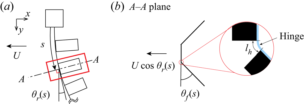
Figure 3. (a) Side view of the elastic structure during the recovery stroke in the  $(x,y)$ plane. (b) Cross-sectional view of the deflected side flaps in the $A$–
$A$– $A$ plane marked in (a). Here, $\theta _{r}$ is the deflection angle of the centre rod, and $\theta _{f}$ is the deflection angle of the side flap.
The fluid-induced torque  $T$ should be balanced by the internal torque of the hinge, which can be modelled as a torsional spring. According to Wu et al. (Reference Wu, Nowak and Breuer2019), the torsional stiffness of a short elastic sheet (i.e. a hinge in our study) takes the form $B_{h}/l_{h}$, where $B_{h}$ and $l_{h}$ are the bending stiffness and length of the hinge, respectively (figure 3b). Then the torque due to the linear torsional spring is $(B_{h}/l_{h})\theta _{f}$. To compensate for the nonlinearity of the relation between the flow-induced torque and the structural deformation, we assume that $(B_{h}/l_{h})\theta _{f}$ is multiplied by a trigonometric function $\cos \theta _{f}$ as follows:
 \begin{equation} \frac{B_{h}}{l_{h}}\,\theta_{f} \cos \theta_{f} = \frac{1}{2}\,C_{N} \rho_{w} w_{f}l_{f} (U \cos \theta_{f} \cos \theta_{r})^2\,\frac{1}{2}\,l_{f}, \end{equation}
where  $B_{h}$ is obtained from $B_{h} = E_{h}I$ (table 3). Young's modulus $E_{h}$ of the hinge was measured in a uniaxial tensile test using a universal tensile testing machine (AGX-V, Shimadzu), and the second moment of area $I$ was calculated using the dimensions of the hinge.
Table 3. Bending stiffness  $B_{h}$ of three hinge types.
The use of a trigonometric function in (3.1) is based on empirical observations. The linear spring relation  $(B_{h}/l_{h})\theta _{f}$ balanced with the flow-induced torque $T$ can be reasonably fitted to the experimental results for small deflections occurring at low $U$. However, as $U$ increases, the balance equation diverges from the experimental results, where $\theta _{f}$ at a given $U$ is underestimated; i.e. the torque required for the side flap to be deflected by $\theta _{f}$ is overestimated. The experimental results show a gradual decrease in the growth rate of the torque to achieve a greater deflection angle $\theta _{f}$. Therefore, for the relation to hold for the higher range of $U$, the left-hand side of (3.1) requires an additional function of $\theta _{f}$ that decreases as $\theta _{f}$ increases. We found that the addition of $\cos \theta _{f}$ in (3.1) could eliminate the error in the high- $U$ range, yielding a better approximation of the internal torque; the validity of the model will be addressed later, in figure 4.

Figure 4. (a) Hinge angle  $\theta _{f}$ obtained from experiment ( $\square$) and theoretical prediction using (3.1) (solid lines). (b) Drag force obtained from force transducer measurement ( $\Diamond$) and theoretical prediction using (3.1) and (3.2) (solid lines). Red, blue and black correspond to hard, medium and soft hinges, respectively. Straight centre rods with $\theta _{r} = 0$ are used to neglect the effect of centre-rod deflection on the folding of the side flaps.
To solve (3.1) and find  $\theta _{f}$, the values of the normal force coefficient $C_{N}$ and hinge length $l_{h}$ need to be determined a priori. The geometry of the side flap is rectangular, with aspect ratio $l_{f}/w_{f}$ between 2 and 4. Although the value of $C_{N}$ for a rectangular flat plate varies with the angle of incidence and the aspect ratio (Tavallaeinejad, Païdoussis & Legrand Reference Tavallaeinejad, Païdoussis and Legrand2018), a constant $C_{N}$ value of 1.95 was used by Luhar & Nepf (Reference Luhar and Nepf2011) to model the dynamics of elastic blades with aspect ratio ranging from 5 to 25 in steady flow. In a later study by Luhar & Nepf (Reference Luhar and Nepf2016), implementation of a constant $C_{N}$ value for a two-dimensional plate from the work of Keulegan & Carpenter (Reference Keulegan and Carpenter1958) was successful in modelling the dynamics of elastic plates with aspect ratios ranging from 2.5 to 10, showing that the use of a constant coefficient value is plausible in modelling reconfiguration under quasi-steady conditions, even for relatively low-aspect-ratio plates. Moreover, Fernando & Rival (Reference Fernando and Rival2016) and Tavallaeinejad et al. (Reference Tavallaeinejad, Païdoussis and Legrand2018) suggested a steady-state $C_{N}$ value of approximately 1.9 for plates oriented normal to the flow. On the basis of these previous studies, the assumption $C_{N} = 2$ appears to be acceptable for our side flap with aspect ratio between 2 and 4.
As mentioned earlier, the deflection of the hinge occurs within a very narrow region less than  $O(10^{-1})$ cm in length. Due to the difficulty of measuring the hinge length directly, its value should be estimated with an alternative experimental approach. A set of experiments to determine the hinge length was conducted using an elastic structure similar to that shown in figure 1(b) for all three hinge types, but with a centre rod sufficiently rigid that it remained vertically straight under translational motion, with only the side flaps being deflected backwards. This is equivalent to $\theta _{r} = 0$ along the entire length of the centre rod. To obtain the deflection angles of the side flaps, a high-speed camera was placed below the water tank to capture directly the deflected side flaps. Although the hinges were made as uniform as possible, a slight variation in the deflection angle among the side flaps was observed, thus the averaged value of the deflection angles was used.
For a translational speed  $U$ between 4 and 60 cm s $^{-1}$, the deflection angles obtained from the filmed images are presented in figure 4(a) as square symbols; the last four data points in $U = 48$–60 cm s $^{-1}$ for the soft hinge type are excluded because of periodic oscillations observed only in these cases. With the value of the hinge length $l_{h}$ set as 0.085 cm, the theoretical prediction using (3.1) (solid lines in figure 4a) fits the experimental measurements well.
To verify further our theoretical approach for the hinge model, drag forces along the  $x$ axis were measured using a force transducer for the aforementioned vertically straight centre rod with deflected side flaps, and they are compared in figure 4(b) with those predicted by integrating (3.2) over the whole elastic structure. The normal force acting on the elastic structure per unit longitudinal length of the centre rod in regions without side flaps is given by $\frac {1}{2} C_{N} \rho _{w} w_{r} (U \cos \theta _{r})^2$. Where side flaps are present, from the normal fluid force (3.1) acting on a side flap, the component of the normal force acting on the two side flaps in the direction normal to the centre rod is given by $\frac {1}{2} C_{N} \rho _{w} (2l_{f}) (U \cos \theta _{r} \cos \theta _{f})^2 \cos \theta _{f}$, where the extra factor $\cos \theta _{f}$ ensures that only the component normal to the centre rod is considered. In regions with side flaps, this term should be added to the normal fluid force exerted on the centre rod per unit length. Thus the normal force $f_{nor}$ acting on the elastic structure per unit longitudinal length of the centre rod is given by
 \begin{equation} f_{nor} =\begin{cases}
\frac{1}{2} C_{N} \rho_{w} w_{r} (U \cos \theta_{r})^2 &
\textrm{for regions without side flaps}, \\
\frac{1}{2} C_{N} \rho_{w} (w_{r} + 2l_{f} \cos ^3
\theta_{f}) (U \cos \theta_{r})^2 & \textrm{for regions
with side flaps}. \end{cases}
\end{equation}
\begin{equation} f_{nor} =\begin{cases}
\frac{1}{2} C_{N} \rho_{w} w_{r} (U \cos \theta_{r})^2 &
\textrm{for regions without side flaps}, \\
\frac{1}{2} C_{N} \rho_{w} (w_{r} + 2l_{f} \cos ^3
\theta_{f}) (U \cos \theta_{r})^2 & \textrm{for regions
with side flaps}. \end{cases}
\end{equation}
Because straight centre rods are used in the cases shown in figure 4(b),  $\theta _{r} = 0$ for these particular cases. In figure 4(b), solid lines are obtained by substituting $\theta _{f}$ values from (3.1) (solid lines in figure 4a) into (3.2). In summary, the theoretical model of the hinge can predict successfully the drag exerted on the entire structure, as well as the deflection angle of the side flap. Our empirical model (3.1) has a shortcoming. Extreme side-flap deflection, close to $\theta _{f}=90^{\circ }$, results in a significant decrease in the term on the left-hand side of (3.1). This is contradictory to the fact that larger deflection induces greater internal bending torque. However, such extreme deflection is limited to some cases with soft hinges and high speed $U$.
$U$.
3.2. Coupling of side-flap and centre-rod deflections
With the hinge model proposed in § 3.1, the deformation of the elastic structure in translational motion is now examined analytically, using an approach similar to those of previous studies (Luhar & Nepf Reference Luhar and Nepf2016; Leclercq & de Langre Reference Leclercq and de Langre2018). The unsteady force-balance equation of the centre rod, which consists of internal bending force/tensile force, external hydrodynamic force, buoyancy force and inertial force, is modelled based on the nonlinear elastica theory:
 \begin{align} & B_{r}\,\frac{\partial^2 \theta_{r}(s,t)}{\partial s^2} + {\rm i} T + \exp({-{\rm i}\theta_{r}(s,t)}) \nonumber\\ &\qquad \times\left[ \int_{s}^{l_{r}} f_{nor}(s^*,t) \exp({{\rm i}\theta_{r}(s^*,t)})\, \mathrm{d} s^* - {\rm i}\,{\Delta} \rho\,gh \int_{s}^{l_{r}}(w_{r} + 2l_{sf})\,\mathrm{d} s^* \right] \nonumber\\ &\quad = \exp({-{\rm i}\theta_{r}(s,t)}) \int_{s}^{l_{r}} f_{I}(s^*,t)\,\mathrm{d} s^*, \end{align}
where  $s$ is the curvilinear coordinate from the clamped end along the axis of the centre rod (figure 3a), and ${\rm i}$ is an imaginary unit. Also, $T$ denotes the tensile force, $\Delta \rho$ is the density difference between the structure $\rho _{s}$ and water $\rho _{w}$, and $l_{sf}$ is the shape function defined in (2.2); $f$ is used to denote several loads, in the form of force per unit length, $f_{nor}$ is the external hydrodynamic load composed of the resistive force based on quasi-steady flow assumption and the added-mass force, whose direction is normal to the surface of the centre rod, and $f_{I}$ is the inertial load from the acceleration of the structure itself. Here, $f_{nor}$ and $f_{I}$ are composed of both centre-rod and side-flap components:
 $$\begin{gather} f_{nor} = f_{R,r} + f_{R,f} + f_{A,r} + f_{A,f}, \end{gather}$$
 $$\begin{gather}f_{I} = f_{I,r} + f_{I,f} , \end{gather}$$
where the subscripts  ${R}$, ${A}$ and ${I}$ denote resistive, added-mass and inertial loads, respectively. Also, as used previously, the subscripts ${r}$ and ${f}$ indicate the centre rod and the side flaps, respectively.
The external and inertial loads acting on the centre rod are given as
 $$\begin{gather} f_{R,r} = \frac{1}{2}\,C_{N}\rho_{w} w_{r}\,| {\rm Re}(U_{r}\exp({-{\rm i}\theta_{r}}))|\, {\rm Re}(U_{r}\exp({-{\rm i}\theta_{r}})), \end{gather}$$
 $$\begin{gather}f_{A,r} = \frac{\rm \pi}{4}\,C_{M} \rho_{w} w_{r}^2\,{\rm Re}(\dot U_{r}\exp({-{\rm i}\theta_{r}})), \end{gather}$$
 $$\begin{gather}f_{I,r} = \rho_{s} hw_{r} \ddot{z}, \end{gather}$$
where  $U_{r}$ denotes the relative flow velocity of the centre rod ( $U_{r}= U-\dot {z}$), the dot denotes a time derivative, and $z= x + {\rm i}y$ is the position of the centre rod on the complex plane in the Cartesian coordinate system. For unsteady motion of the elastic structure, the normal force coefficient $C_{N}$ and added-mass force coefficient $C_{M}$ will vary locally by the Keulegan–Carpenter number $KC$ (Keulegan & Carpenter Reference Keulegan and Carpenter1958). Instead of $C_{N} = 2$ used for the quasi-steady condition, $C_{N}$ dependent on $KC$ is used for unsteady simulations: $C_{N} = \max (10KC^{-1/3},1.95)$ from Luhar & Nepf (Reference Luhar and Nepf2016). However, the value of $C_{M}$ with respect to $KC$ cannot be determined simply. Therefore, a constant value $C_{M} = 1$ is chosen in this study for simplification, which is identical to the approach adopted by Leclercq & de Langre (Reference Leclercq and de Langre2018). According to the earlier study by Luhar & Nepf (Reference Luhar and Nepf2016), a constant value $C_{M} = 1$ did not alter the results significantly.
On the other hand, the force acting on the side flap is determined by integrating the individual load along the lengthwise direction of the side flap. The external and inertial loads acting on the side flaps are given as
 \begin{align} f_{R, f} &= C_{N}\rho_{w} \cos \theta_{f} \int_0^{l_{sf}} | U_{f} - \dot\theta_{f}l^*|\, (U_{f}-\dot{\theta_{f}} l^*)\,\mathrm{d}l^* \nonumber\\ &= \frac{1}{3}\,C_{N}\rho_{w} \cos \theta_{f} l_{sf} [\hat{l}_{f1} U_{f}^2 + |U_{f}-\dot\theta_{f} l_{sf}|\,(2U_{f} - \dot\theta_{f}l_{sf})], \end{align}
 \begin{align} f_{A, f} &=
\frac{\rm \pi}{2}\,C_{M} \rho_{w} w_{f} \cos\theta_{f}
\int_0^{l_{sf}} (\dot U_{f} - \ddot \theta_{f} l^*
)\,\mathrm{d} l^* \nonumber\\ &= \frac{\rm \pi}{2}\,C_{M}
\rho_{w} w_{f} \cos\theta_{f} l_{sf} \left( \dot
U_{f}-\frac{1}{2}\,\ddot\theta_{f}l_{sf} \right),
\end{align}
\begin{align} f_{A, f} &=
\frac{\rm \pi}{2}\,C_{M} \rho_{w} w_{f} \cos\theta_{f}
\int_0^{l_{sf}} (\dot U_{f} - \ddot \theta_{f} l^*
)\,\mathrm{d} l^* \nonumber\\ &= \frac{\rm \pi}{2}\,C_{M}
\rho_{w} w_{f} \cos\theta_{f} l_{sf} \left( \dot
U_{f}-\frac{1}{2}\,\ddot\theta_{f}l_{sf} \right),
\end{align}
 \begin{align}
f_{I,f} &= 2\rho_{s}h \int_0^{l_{sf}}[\ddot{z} +(\ddot\theta_{f}\cos\theta_{f}+
\dot\theta_{f}^2 \sin\theta_{f})l^*]\mathrm{d} l^* \nonumber\\ &= 2\rho_{s}h
l_{sf}\left[\ddot{z} + \frac{l_{sf}}{2}\,(\ddot\theta_{f}
\cos\theta_{f} + \dot\theta_{f}^2 \sin\theta_{f} )\right].
\end{align}
\begin{align}
f_{I,f} &= 2\rho_{s}h \int_0^{l_{sf}}[\ddot{z} +(\ddot\theta_{f}\cos\theta_{f}+
\dot\theta_{f}^2 \sin\theta_{f})l^*]\mathrm{d} l^* \nonumber\\ &= 2\rho_{s}h
l_{sf}\left[\ddot{z} + \frac{l_{sf}}{2}\,(\ddot\theta_{f}
\cos\theta_{f} + \dot\theta_{f}^2 \sin\theta_{f} )\right].
\end{align}
Here,  $U_{f}$ and $\dot U_{f}$ denote the relative flow velocity and acceleration at the hinge-connected end of the side flap, in the direction normal to the side-flap orientation:
 $$\begin{gather} U_{f} = {\rm Re}(U_{r}\exp({-{\rm i}\theta_{r}})) \cos\theta_{f}, \end{gather}$$
 $$\begin{gather}\dot U_{f} = {\rm Re}(\dot U_{r}\exp({-{\rm i}\theta_{r}})) \cos\theta_{f}. \end{gather}$$
Also,  $\hat {l}_{f1}$ in (3.6a) is defined as follows to express different integrated forms, depending on the motion of the side flap:
 \begin{equation}
\hat {l}_{f1} =\begin{cases}
(|U_{f}|-|U_{f}-\dot\theta_{f} l_{sf}|)/\dot\theta_{f} l_{sf} & \textrm{if } \dot\theta_{f} \neq 0,\\
1 & \textrm{if } \dot\theta_{f} = 0\ \&\ U_{f}>0,\\
-1 & \textrm{if } \dot\theta_{f} = 0\ \&\ U_{f}<0. \end{cases}
\end{equation}
\begin{equation}
\hat {l}_{f1} =\begin{cases}
(|U_{f}|-|U_{f}-\dot\theta_{f} l_{sf}|)/\dot\theta_{f} l_{sf} & \textrm{if } \dot\theta_{f} \neq 0,\\
1 & \textrm{if } \dot\theta_{f} = 0\ \&\ U_{f}>0,\\
-1 & \textrm{if } \dot\theta_{f} = 0\ \&\ U_{f}<0. \end{cases}
\end{equation}
Moreover, from the definition of  $l_{sf}$ in (2.2), the loads induced by the side flaps ( $f_{R,f}$, $f_{A,f}$ and $f_{I,f}$) are eliminated for the regions without the side flaps in which $l_{sf} = 0$.
With the complete set of relations describing the loads acting on the centre rod and side flaps provided, we can find that when the centre rod is rigid ( $\theta _{r}=0$) and the motion is steady ( $\dot \theta _{f}=0$), $\hat {l}_{f1}$ is 1, and the relative flow velocities normal to the centre rod ( ${\rm Re}(U_{r}\exp ({-{\rm i}\theta _{r}}))$) and the side flaps ( $U_{f}$) become $U$ and $U\cos \theta _{f}$, respectively. Eventually, (3.4a) becomes identical to (3.2).
Next, for the dynamics of the side flaps, the deflection angle of the side flap,  $\theta _{f}$, is evaluated from the following unsteady torque-balance equation for the hinge, which is extended from the quasi-steady (3.1):
 \begin{equation} {-}\frac{B_{h}}{l_{h}}\,\theta_{f} \cos \theta_{f} +\tau_{R}+\tau_{A}+\tau_{B}= \tau_{I}, \end{equation}
where the first term on the left-hand side is the bending moment of the hinge described in § 3.1, and  $\tau _{R}$, $\tau _{A}$, $\tau _{B}$ and $\tau _{I}$ are the torques induced by the resistive, added-mass, buoyancy and inertial forces, respectively. The value of $\theta _{f}$ for each side flap can be estimated individually since the side flaps are not connected to each other. We have
 \begin{align} \tau_{R} &= \frac{1}{2}\,C_{N} \rho_{w} w_{f} \int_0^{l_{sf}} |U_{f} - \dot\theta_{f} l^* |\,(U_{f} - \dot\theta_{f} l^*) l^* \,\mathrm{d} l^* \nonumber\\ &= \frac{1}{24}\,C_{N} \rho_{w} w_{f} l_{sf}^2 [\hat{l}_{f2}U_{f}^2 + |U_{f}-\dot\theta_{f} l_{sf}|\,(5U_{f}-3\dot\theta_{f} l_{sf})], \end{align}
 \begin{align} \tau_{A} &= \frac{\rm \pi}{4}\,C_{M} \rho_{w} w_{f}^2 \int_0^{l_{sf}} ( \dot U_{f} - \ddot \theta_{f} l^* )l^*\,\mathrm{d} l^* \nonumber\\ &= \frac{\rm \pi}{24}\,C_{M} \rho_{w} w_{f}^2 l_{sf}^2 ( 3\dot U_{f} - 2\ddot \theta_{f} l_{sf} ), \end{align}
 \begin{equation} \tau_{B} ={-}\frac{1}{2}\,\Delta \rho\,g w_{f} h l_{sf} ^2 \sin\theta_{r}\cos \theta_{f}, \end{equation}
 \begin{align}
\tau_{I} &= \rho_{s}h w_{f} \int_0^{l_{sf}}\left[\ddot{z}
\cos \theta_{f} + \ddot\theta_{f} l^*\right]l^* \,\mathrm{d} l^*\nonumber\\
&= \rho_{s}h w_{f} l_{sf}^2 \left[\frac{1}{2}\,\ddot{z} \cos
\theta_{f} + \frac{1}{3}\,\ddot\theta_{f} l_{sf} \right],
\end{align}
\begin{align}
\tau_{I} &= \rho_{s}h w_{f} \int_0^{l_{sf}}\left[\ddot{z}
\cos \theta_{f} + \ddot\theta_{f} l^*\right]l^* \,\mathrm{d} l^*\nonumber\\
&= \rho_{s}h w_{f} l_{sf}^2 \left[\frac{1}{2}\,\ddot{z} \cos
\theta_{f} + \frac{1}{3}\,\ddot\theta_{f} l_{sf} \right],
\end{align}
where  $\hat {l}_{f2}$ is defined as
 \begin{equation}
\hat{l}_{f2} =\begin{cases} \dfrac{1}{\dot\theta_{f} l_{sf}}
\left[U_{f}\, \dfrac{|U_{f}|-|U_{f}-\dot\theta_{f}
l_{sf}|}{\dot\theta_{f} l_{sf}} - |U_{f}-\dot\theta_{f}
l_{sf}|\right] & \textrm{if } \dot\theta_{f} \neq 0, \\
1 & \textrm{if } \dot\theta_{f} = 0 \ \& \ U_{f}>0, \\
{-1} & \textrm{if } \dot\theta_{f} = 0 \ \& \ U_{f}<0.
\end{cases} \end{equation}
\begin{equation}
\hat{l}_{f2} =\begin{cases} \dfrac{1}{\dot\theta_{f} l_{sf}}
\left[U_{f}\, \dfrac{|U_{f}|-|U_{f}-\dot\theta_{f}
l_{sf}|}{\dot\theta_{f} l_{sf}} - |U_{f}-\dot\theta_{f}
l_{sf}|\right] & \textrm{if } \dot\theta_{f} \neq 0, \\
1 & \textrm{if } \dot\theta_{f} = 0 \ \& \ U_{f}>0, \\
{-1} & \textrm{if } \dot\theta_{f} = 0 \ \& \ U_{f}<0.
\end{cases} \end{equation}
The detailed numerical procedure for solving (3.3) in terms of  $\theta _{r}$ and (3.9) in terms of $\theta _{f}$ is described in Appendix A.
3.3. Simplification for quasi-steady motion
The full dynamic model derived in § 3.2 is simplified to represent the quasi-static interaction of the elastic structure with the flow. For steady translation with constant speed  $U = U_0$ during either the power stroke or the recovery stroke and resultant quasi-static deformation, time derivative terms $\dot \theta _{r}$ and $\dot \theta _{f}$ are assumed to be zero, yielding zero added-mass and inertial loads. Consequently, the real components in (3.3) are simplified as
 \begin{align} & B_{r}\,\frac{\mathrm{d}^2 \theta_{r}(s)}{\mathrm{d}s^2} + \int_{s}^{l_{r}} [f_{R,r}(s^*) + f_{R,f}(s^*)] \cos (\theta_{r}(s) - \theta_{r}(s^*))\,\mathrm{d} s^* \nonumber\\ &\quad -\Delta \rho\,gh \sin \theta_{r}(s) \int_{s}^{l_{r}} (w_{r} + 2l_{sf})\, \mathrm{d} s^* = 0, \end{align}
which is similar to the forms given by Gosselin et al. (Reference Gosselin, de Langre and Machado-Almeida2010), Luhar & Nepf (Reference Luhar and Nepf2011) and Pezzulla et al. (Reference Pezzulla, Strong, Gallaire and Reis2020). Since the model is for steady translation, (3.1) can be used directly to obtain  $\theta _{f}$.
To solve (3.12) and (3.1) simultaneously, and find  $\theta _{r}$ and $\theta _{f}$, the centre rod is discretized into equally spaced segments each of length $\Delta s$ along the $s$ axis: $\Delta s = l_{r}/N$, where $N = 20$. With the central difference scheme being used for the differential term and the mensuration by parts for the integral terms, (3.12) becomes
 \begin{align} & B_{r}\,\frac{\theta_{{r},j+1} - 2\theta_{{r},j} + \theta_{{r},j-1}}{(\Delta s)^2} + \sum_{k=j+1}^{N} (f_{{R,r},k} + f_{{R,f},k}) \cos (\theta_{{r},j} - \theta_{{r},k})\,\Delta s \nonumber\\ &\quad - \Delta \rho\,gh \sin \theta_{{r},j} \sum_{k=j+1}^{N} (w_{r} + 2l_{{sf},k})\, \Delta s = 0,\quad j = 1, \ldots, N-1. \end{align}
With the boundary conditions  $\theta _{r} = 0$ at $s = 0$ ( $j = 0$) and $\mathrm {d}\theta _{r}/\mathrm {d}s = 0$ at $s = l_{r}$ ( $j = N$), iterations were performed to solve the boundary value problem using Newton's method until the left-hand side of (3.13) fell below $10^{-5}$ times the second term in (3.12) at every node.
4. Results and discussion
4.1. Reconfiguration of the elastic structure under quasi-steady motion
The quasi-static deformation of the elastic structure under steady translation ( $U = U_0$) is first considered in §§ 4.1–4.3. A notable feature in the quasi-static deformation is the difference in the orientation of the side flaps along the longitudinal direction of the centre rod (along the curvilinear coordinate $s$ in figure 3) between the power stroke and the recovery stroke. Although the centre rod bends backwards during the power stroke, the motion of the side flaps is constrained by the unidirectional hinge, and they remain almost straight with respect to the centre rod, without deflection (see figures 5a-i,b-i). Thus, regardless of the hinge type, the deflections of the centre rod are similar. By contrast, owing to the deflection of the side flaps during the recovery stroke and the consequent reduction in the projection area normal to the direction of translation, less drag is exerted on the structure during the recovery stroke than the power stroke, resulting in less deflection of the centre rod (see figures 5a-ii,b-ii). Because the reconfiguration of the centre rod causes a reduction in the magnitude of the relative flow velocity normal to the elastic structure along the longitudinal direction, $\theta _{f}$ values of the side flaps decrease as well along the longitudinal direction, as shown clearly in figure 5(b-ii).

Figure 5. Raw images of the deformed elastic structure during (i) the power stroke and (ii) the recovery stroke: (a) soft-hinge case (s4), and (b) medium-hinge case (m4), in table 2. Here,  $U = 40$ cm s $^{-1}$. See the supplementary movies available at https://doi.org/10.1017/jfm.2022.970.
We now compare the deflection profiles of the centre rod as estimated by the theoretical model in § 3.3 with experimental results. The deflection profiles of the thin-centre-rod cases with soft hinges are exemplified in figure 6. With varying side-flap length  $l_{f}$, the deflection profiles can be predicted to a reasonable extent. As well as the centre rod, the deflection angles of the side flaps for the cases presented in figures 5 and 6 also show a good match between the experimental results and theoretical estimates (figure 7). These results indicate that our theoretical model incorporating two deflecting parts, namely the centre rod and hinges, is appropriate for characterizing the quasi-static dynamics of the elastic structure.

Figure 6. Deflection profiles of the thin centre rod with soft hinges (cases s2, s3 and s4 in table 2) for (a) the power stroke and (b) the recovery stroke, where (i) is from the experimental measurement, and (ii) is from the theoretical model. Black, blue and red indicate  $l_{f} = 4$, 3 and 2 cm, respectively. In each panel, the three lines of each colour correspond to the cases with $U = 12$, 32 and 52 cm s $^{-1}$, respectively; backward deformation is greater for larger $U$.
$U$.

Figure 7. Deflection angle  $\theta _{f}$ of the 10 side flaps along the longitudinal direction of the centre rod during the recovery stroke, for: (a) the s4 ( $\square$) and m4 ( $\Diamond$) cases with $U = 40$ cm s $^{-1}$ (the cases shown in figures 5a-ii,b-ii); (b) the s2 ( $\circ$, thin line) and s4 ( $\square$, thick line) cases with $U = 12$ cm s $^{-1}$ (blue) and 52 cm s $^{-1}$ (red) (the cases shown in figures 6b-i to b-ii). Symbols indicate experimental measurements, and short horizontal lines indicate theoretical estimates.
In previous studies of the reconfiguration of elastic bodies under steady flow, the Cauchy number  $C_Y$ was introduced to characterize the deformation of the body subjected to the flow (e.g. de Langre Reference de Langre2008; Gosselin et al. Reference Gosselin, de Langre and Machado-Almeida2010; Whittaker et al. Reference Whittaker, Wilson and Aberle2015; Leclercq & de Langre Reference Leclercq and de Langre2016). This number is defined as the ratio of inertial fluid force to elastic force: $C_Y = \rho _{f} U^2/E$, where $\rho _{f}$ and $E$ are the fluid density and Young's modulus of the elastic body, respectively. Similarly, a dimensionless flow velocity in the form
 \begin{equation} \eta = U\left(\frac{\rho_{f} L^3 f}{B}\right)^{1/2}, \end{equation}
which indicates the relative magnitudes of the inertial fluid force and the bending force of the elastic body, has been suggested by several studies (e.g. Alben et al. Reference Alben, Shelley and Zhang2002; Shelley & Zhang Reference Shelley and Zhang2011; Kim et al. Reference Kim, Cossé, Cerdeira and Gharib2013; Kim, Kang & Kim Reference Kim, Kang and Kim2017). In (4.1),  $B$ is the bending stiffness, $L$ is a characteristic length, and $f$ is a geometric parameter that determines the effective cross-sectional width of the elastic body. In the present study, a modified version of the dimensionless flow velocity is proposed in which $f$ is replaced with a combination of $w_{r}$, $l_{f}$ and $\theta _{f}$ to give a more appropriate characterization of the elastic deformation.
Because the drag force scales roughly with the projection area of the structure on the plane normal to the direction of translation, its magnitude is determined by the geometric parameters of the centre rod and the side flaps, such as  $l_{r}$, $w_{r}$, $l_{f}$, $w_{f}$, $\theta _{r}$ and $\theta _{f}$. Along with the fixed values of $l_{r}$, $w_{r}$ and $w_{f}$, the parameter varied in the present study is the side-flap length $l_{f}$, with the deflection angle of the centre rod, $\theta _{r}$, and those of the individual side flaps, $\theta _{f}$, being dependent on various experimental parameters. In the quasi-static theoretical model, the normal force acting on the elastic structure per unit length was defined as (3.2), where $w_{r}$ and $l_{f} \cos ^3 \theta _{f}$ can be considered as the effective cross-sectional widths of the centre rod and the side flap, respectively. Although the value of $\theta _{f}$ decreases along the longitudinal direction of the centre rod owing to the reduction in the normal component of the flow relative to the deformed centre rod (figures 5b-ii and 7), the value of $\theta _{f}$ when the centre rod is vertically straight and rigid ( $\theta _{r} = 0$), and completely perpendicular to the relative flow, is chosen as a reference $\theta _{f}$ for simplicity and is denoted by $\theta _{f,ref}$. This value can be estimated with reasonable accuracy using (3.1); the limitations of such a choice will be discussed later. Therefore, $l_{f} \cos ^3 \theta _{f,ref}$ is determined for each case, and $\theta _{f,ref}$ differs between the power and recovery strokes; $\theta _{f,ref} = 0$ for the power stroke.
The effective area of the centre rod scales with  $w_{r} l_{r}$, and that of all the side flaps scales with $N_{f} w_{f}l_{f} \cos ^3 \theta _{f,ref}$, where $N_{f} = 20$ is the total number of the side flaps (10 for each side). By dividing the effective area by the centre-rod length $l_{r}$, the effective cross-sectional width of the elastic structure is expressed as $(w_{r}l_{r} + N_{f} w_{f}l_{f} \cos ^3 \theta _{f,ref})/l_{r}$. Replacing $f$ and $L$ in (4.1) with the defined effective cross-sectional width and the centre-rod length, respectively, we propose the following dimensionless speed for characterizing the reconfiguration of our model that accompanies the deformations of the centre rod and the hinges together:
 \begin{equation} U^* = U\left[ \frac{\rho_{w} l_{r}^2 (w_{r}l_{r} + N_{f} w_{f}l_{f} \cos^3 \theta_{f,ref})}{B_{r}} \right]^{1/2}. \end{equation}
 For a more quantitative analysis of the structural deformation, the amplitude of tip deflection along the  $x$ axis is examined (figure 8). Overall, the results of the theoretical model are in good agreement with those of the experimental measurements. Notably, the dimensionless tip deflection $\delta /l_{r}$ is well characterized by the newly defined dimensionless speed $U^*$ in (4.2); the plots of the dimensional tip deflection $\delta$ with respect to the dimensional speed $U$ are provided in Appendix B. Regardless of the variations in the side-flap length and hinge type, $\delta /l_{r}$ tends to collapse onto a single curve. Because the numerator of $U^*$ scales with the drag acting on the elastic structure for both power and recovery strokes, and takes the effect of the deformed hinges into account, a similar degree of tip deflection is observed at the same $U^*$ value between the two strokes, as can be seen from a comparison of the (i) and (ii) panels of figure 8. Furthermore, it is worth mentioning that because the thickness of the centre rod is included in $B_{r}$ in the denominator of $U^*$ (4.2), the tip deflections in the thin-centre-rod cases (figures 8a-i,ii) and the thick-centre-rod cases (figures 8b-i,ii) also show similar values at the same $U^*$; note that the range of the $x$ axis differs between figures 8(a) and 8(b).

Figure 8. Amplitude of tip deflection  $\delta /l_{r}$ for (a) cases with a thin centre rod (small letters in table 2), and (b) cases with a thick centre rod (capital letters in table 2), where (i) and (ii) are for the power and recovery strokes, respectively. Symbols and lines denote experimental and theoretical results, respectively.
However, a diverging trend of  $\delta /l_{r}$ with variations in $l_{f}$ and $B_{h}$ is observed during the recovery stroke in the relatively high- $U^*$ regime (figures 8a-ii,b-ii). This divergence originates from the aforementioned limitation in the way $U^*$ was defined using $\theta _{f,ref}$ of a straight centre rod. As illustrated in figures 5(b-ii) and 7(a), the deflection angle of the side flap varies dramatically along the longitudinal direction of the centre rod when the rod undergoes large deflection, i.e. during the recovery stroke at high $U^*$. That is, the single reference value of $\theta _{f,ref}$ used to define $U^*$, which was obtained from the case with the straight centre rod, cannot represent the actual deflection angle of the side flap in such cases. As can be inferred from (3.1), the cases with larger $l_{f}$ and smaller $B_{h}$ generally lead to greater values of $\theta _{f}$. Moreover, more distinct variations in $\theta _{f}$ along the longitudinal direction of the centre rod originate from larger deflection of the rod. Consequently, the $\delta /l_{r}$ values for high $U^*$ tend to diverge from the collapsed curve, in contrast to figures 8(a-i,b-i).
4.2. Drag of the elastic structure
The drag force acting on the elastic structure is correlated with its reconfiguration. Here, using a scaling analysis, we examine how the drag force changes with the experimental parameters considered in this study, particularly with the dimensionless speed  $U^*$ that characterizes the reconfiguration of the elastic structure. The reconfiguration number $\mathcal {R}$ (Gosselin et al. Reference Gosselin, de Langre and Machado-Almeida2010), representing the ratio of the actual drag $D$ exerted on a flexible structure to the drag exerted on a rigid one with identical initial geometry, is expressed as
 \begin{equation} \mathcal{R} = \frac{D}{\tfrac{1}{2}\rho_{f} A C_{N} U^2}, \end{equation}
where  $A$ denotes the projection area on the plane normal to the incoming flow for the initial configuration. Since the geometry under consideration is initially normal to the direction of translation, $C_{N}$ is used in the denominator of (4.3) instead of $C_{D}$.
Using the definition in (4.3), the trend of the reconfiguration number  $\mathcal {R}$ with respect to the dimensionless speed $U^*$ is depicted in figure 9 for the cases of steady translation; note that the range of the $x$ axis differs between figures 9(a) and 9(b). The plots of the dimensional quasi-steady drag $D$ with respect to the dimensional speed $U$ are also provided in Appendix B. The values of the drag computed with the theoretically estimated profile are in reasonable agreement with those acquired directly from force transducer measurements with the same parameters, particularly for the power stroke. Because there are no side-flap deflections for the power stroke, the reconfiguration number $\mathcal {R}$ is hardly affected by the hinge type (hinge stiffness $B_{h}$) and side-flap length $l_{f}$, showing a collapsed curve (figures 9a-i,b-i). By contrast, for the recovery stroke, diverse trends exist due to the deflection of the side flaps as $B_{h}$ and $l_{f}$ vary (figures 9a-ii,b-ii). Overall, a more dramatic decrease in drag with increasing $U^*$ is observed compared with the power stroke, and the effect of drag reduction is greater for cases with softer hinges and longer side flaps.

Figure 9. Reconfiguration number  $\mathcal {R}$ for (a) cases with a thin centre rod (small letters in table 2), and (b) cases with a thick centre rod (capital letters in table 2), where (i) and (ii) are for the power and recovery strokes, respectively. Symbols and lines denote experimental and theoretical results, respectively.
While the dramatic decrease in drag during the recovery stroke is expected for the softer hinge with greater side-flap deflection, the trend of drag reduction by the variations in the side-flap length  $l_{f}$ needs more careful examination. It is trivially obvious that the drag $D$ increases with $l_{f}$ at the same translational speed $U$. However, this statement is valid only for the power stroke. Similar to the result shown in figure 4(b) of Gosselin et al. (Reference Gosselin, de Langre and Machado-Almeida2010), the cases with longer side flaps have less drag for the recovery stroke, which is attributed to the increase in $\theta _{f}$. In the defined effective cross-sectional width $(w_{r}l_{r} + N_{f} w_{f}l_{f} \cos ^3 \theta _{f,ref})/l_{r}$ that scales the drag force acting on the elastic structure (4.2), $l_{f}$ and $\theta _{f,ref}$ are in a trade-off relationship. Referring to the formula for the hinge deflection angle (3.1), an increase in $l_{f}$ leads to an increase in $\theta _{f}$. Accordingly, $l_{f} \cos ^3 \theta _{f}$ can become smaller despite a greater $l_{f}$ in certain cases, depending on the magnitudes of parameters such as $B_{h}$ and $l_{h}$, which results in less drag generation.
The definition in (4.3) might be enough if our model were to deform only at the centre rod, as in the case of the power stroke. However, considering the bending of the side flaps observed during the recovery stroke, an alternative definition of the reconfiguration number is desirable. When  $U^*$ was defined in (4.2), the effect of bending the side flaps was considered in the numerator through the term $(w_{r}l_{r} + N_{f} w_{f}l_{f} \cos ^3 \theta _{f,ref})/l_{r}$. In a similar way, $A$ in the denominator of (4.3) is replaced by $w_{r}l_{r} + N_{f} w_{f}l_{f} \cos ^3 \theta _{f,ref}$, which is the effective area subjected to a uniform speed $U$. Therefore, the form of the reconfiguration number appropriate to our model is
 \begin{equation} \mathcal{\hat{R}} = \frac{D}{\tfrac{1}{2}\rho_{w} (w_{r}l_{r} + N_{f} w_{f}l_{f} \cos^3 \theta_{f,ref}) C_{N} U^2}. \end{equation}
 In figure 10, the trend of the newly defined reconfiguration number  $\mathcal {\hat {R}}$ is shown with respect to $U^*$ for both the power and recovery strokes and for several side-flap lengths and hinge types; note that the range of the $x$ axis differs between figures 10(a) and 10(b). Regardless of the experimental parameters, the magnitude of $\mathcal {\hat {R}}$ is determined solely by $U^*$. This result implies that the effects of the bending stiffness of the centre rod and the hinges, as well as those of the geometry of the structure, on the drag force are reflected well in the definition of $\mathcal {\hat {R}}$. While the tip deflection $\delta /l_{r}$ increases monotonically with $U^*$ (figure 8), the new reconfiguration number $\mathcal {\hat {R}}$ tends to decrease with $U^*$. Accordingly, $\mathcal {\hat {R}}$ has an inverse relationship with $\delta /l_{r}$; see figure 20 in Appendix C. That is, the drag reduction effect of the elastic structure can be predicted using the tip deflection of the centre rod alone, although the reconfiguration is three-dimensional.

Figure 10. New reconfiguration number  $\mathcal {\hat {R}}$ for (a) cases with a thin centre rod (small letters in table 2) and (b) cases with a thick centre rod (capital letters in table 2). (i) and (ii) are for the power and recovery strokes, respectively. Symbols and lines denote experimental and theoretical results, respectively.
In both figures 9 and 10, significant deviations in the experimental results of  $\mathcal {R}$ and $\mathcal {\hat {R}}$ are observed in the regime of low $U^*$ for both power and recovery strokes. The dimensional drag $D$ (figure 19 in Appendix B) is measured reasonably for the low-speed regime. However, from the definition of the reconfiguration number that includes $U^2$ in the denominator, a small error in the measured drag at a low speed leads to significant deviations in $\mathcal {R}$ and $\mathcal {\hat {R}}$.
At this point, limitations of the simple theoretical model need to be addressed in order to explain reasons for the discrepancy in deformation and drag between the theoretical model and experimental measurements. First, the use of a single value of  $C_{N} = 2$, which was addressed in § 3.1, can cause the discrepancy for the three-dimensional rearrangement. Connections between the centre rod and side flaps and the narrow gap between adjacent side flaps are not reflected in the $C_{N}$ value chosen in our study as the value originates from a single isolated plate. Furthermore, the flow velocity normal to the surfaces cannot be determined simply by the three-dimensional orientations of the centre rod and side flaps. Another major cause is the effect of finite thickness of the elastic structure. In the theoretical model, the thickness of the structure is used only to calculate its bending stiffness, and side surfaces, which exist in the actual structure due to finite thickness 1.10–1.75 mm, are not considered. When the actual elastic structure deforms, hydrodynamic force acts not only on the initially normal faces of the side flaps but also on their side surfaces. The contribution by the side surfaces becomes greater for the cases with larger deflection. In addition, skin friction, which is not considered in our model, may cause the discrepancy. However, a skin-friction coefficient of a flat plate is approximately 0.1 for $Re = 100$ and even lower for higher $Re$ (Kundu & Cohen Reference Kundu and Cohen2004; Luhar & Nepf Reference Luhar and Nepf2016), and the effect of skin friction on net drag is insignificant, from a comparison between the scales of skin-friction drag and pressure drag. Moreover, the assumption of quasi-static deformation is no longer valid for the highly deflected side flaps ( $\theta _{f}$ over 80 $^{\circ }$) found in cases with soft hinges with a translational speed $U$ over 50 cm s $^{-1}$. These side flaps with large deflection angles exhibit fluttering motion with an amplitude within 5 $^{\circ }$. Nevertheless, the effect of the fluttering motion on drag is marginal because the deflection angle of the side flaps contributes to the drag in the form $\cos ^3 \theta _{f}$ according to (3.2); $\cos ^3 \theta _{f}$ is less than 0.005 for $\theta _{f}$ over 80 $^{\circ }$.
Next, we evaluate the ratio of drag forces generated during the power and recovery strokes, respectively,  $D_{Power}/D_{Recovery}$, at the same dimensional speed $U$ (figure 11). Although this subsection considers only simple steady motion for the power and recovery strokes, the ratio of the drag forces provides a rough evaluation of the capability to produce net thrust over a cycle under the condition that the time-varying speeds of the power and recovery strokes are identical. Furthermore, the overall trend of the force ratio with respect to $U$ is predictable using the theoretical model.

Figure 11. Force ratio between power and recovery strokes,  $D_{Power}/D_{Recovery}$, versus dimensional translational speed $U$ for cases with (a) a thin centre rod, and (b) a thick centre rod. Symbols and lines are from experimental and theoretical results, respectively. Symbols, line types and colours denote the same parameters as in figures 8 and 10.
Previously, the decrease in drag  $D$ for larger $l_{f}$ during the recovery stroke was explained using the relationship between $l_{f}$ and $\theta _{f}$. By contrast, the drag during the power stroke scales with $w_{r} + l_{f}$ because $\theta _{f} = 0$, and it increases with $l_{f}$. Thus for a pair of power and recovery strokes under the same $U$, the use of larger $l_{f}$ may be a better choice in maximizing the force ratio $D_{Power}/D_{Recovery}$, as shown in figure 11. Moreover, for a soft hinge, a peak value of the force ratio exists in the $U$ range considered in this study. This is because the rates of change in drag force with respect to $U$ differ between the power and recovery strokes, which can be predicted from the difference in the effective width scaling the drag between the power and recovery strokes, $(w_{r}l_{r} + N_{f} w_{f}l_{f})/l_{r}$ and $(w_{r}l_{r} + N_{f} w_{f}l_{f} \cos ^3 \theta _{f,ref})/l_{r}$, respectively.
In describing the reconfiguration during the recovery stroke, we explained how  $\theta _{r}$ and $\theta _{f}$ are coupled. The increase in $\theta _{r}$ along the longitudinal direction of the centre rod is accompanied by an increase in the incidence angle of the relative flow on the side flaps as well, which can lead to a reduction in $\theta _{f}$ along the longitudinal direction of the centre rod during the recovery stroke (figures 5b-ii and 7a). The increase in $B_{r}$ causes less backward deformation of the centre rod (i.e. the overall decrease in $\theta _{r}$ of the centre rod) and weakens the reduction in $\theta _{f}$ along its longitudinal direction during the recovery stroke. That is, for a case with greater $B_{r}$, the side flaps near the centre rod tip can maintain large deflection angles during the recovery stroke, and a greater difference in effective area between the power and recovery strokes is achieved. For the same hinge type, although an increase in $B_{r}$ causes less deformation of the centre rod and contributes to greater drag production of the centre rod, the drag reduction by bending of the side flaps during the recovery stroke is more substantial, which yields an increase in the force ratio, as is seen from a comparison of figures 11(a) and 11(b).
4.3. Extension to extreme conditions
In the preceding subsections, our theoretical model has estimated successfully the reconfiguration and drag force of the elastic structure for both power and recovery strokes. We now extend the range of bending stiffness  $B_{r}$ of the centre rod to show that the reconfiguration and drag force are also characterized by the suggested dimensionless parameters $U^*$ and $\mathcal {\hat {R}}$ in extreme conditions. For the theoretical model, two extreme values of $B_{r}$, namely $0.31\times 10^{-3}$ and 0.31 N m $^{-2}$, were chosen to represent very flexible and stiff centre rods, respectively, which correspond to acrylic sheets of thickness $h = 0.5$ and 5 mm. In this subsection, experimental results are not presented, owing to the difficulty of fabricating very thin or very thick elastic structures with $h = 0.5$ and 5 mm.
The scalings of the dimensionless tip deflection  $\delta /l_{r}$ and reconfiguration number $\mathcal {\hat {R}}$ with the dimensionless speed $U^*$ hold well throughout a much wider range of $U^*$ and predict that the rates of change of the magnitudes of $\delta /l_{r}$ and $\mathcal {\hat {R}}$ gradually decrease with increasing $U^*$ (figure 12). Furthermore, as discussed in connection with figure 11, an increase in $B_{r}$ for a fixed value of $B_{h}$ generally induces a greater force ratio $D_{Power}/D_{Recovery}$ (figure 13); the ratio of $B_{r}$ to $B_{h}$ increases from (a) to (c) in the figure. The black, blue and red horizontal lines in figure 13 indicate the maximum values of the force ratio for $l_{f} = 4$, 3 and 2 cm, respectively, which are obtained from the theoretical model. As $B_{r}$ becomes greater and eventually the deflection of the centre rod becomes negligible for the two strokes, the force ratio approaches the maximum value predicted by the theoretical model at high $U$ (figure 13). The maximum value of the force ratio is essentially the ratio of the projection area of the elastic structure corresponding to $\theta _{f} = 0$ (no folding of the side flaps) during the power stroke to that corresponding to $\theta _{f} = {\rm \pi}/2$ (complete folding of the side flaps) during the recovery stroke, if the effect of the side-flap thickness on drag generation is assumed to be negligible.

Figure 12. Theoretical predictions of (a) dimensionless tip deflection  $\delta /l_{r}$ and (b) reconfiguration number $\mathcal {\hat {R}}$ in a broad range of $U^*$: $B_{r} = 0.31\times 10^{-3}$ N m $^{2}$ (red), $5.49\times 10^{-3}$ N m $^{2}$ (black), and 0.31 N m $^{2}$ (blue). Here, (i) and (ii) are for the power and recovery strokes, respectively.

Figure 13. Force ratio between power and recovery strokes,  $D_{Power}/D_{Recovery}$, of soft-hinge cases versus translational speed $U$: (a) $B_{r} = 0.31\times 10^{-3}$ N m $^{2}$; (b) $B_{r} = 5.49\times 10^{-3}$ N m $^{2}$; (c) $B_{r} = 0.31$ N m $^{2}$. Line types and colours denote the same parameters as in figures 8 and 10. The black, blue and red horizontal lines indicate the theoretical maximum values of the force ratio for $l_{f} = 4$, 3 and 2 cm, respectively.
4.4. Unsteady motions of the elastic structure
Thus far, we have explored the physical aspects of the elastic structure under quasi-steady loading. While the results of quasi-static deformation have provided insight to understand how three-dimensional reconfiguration is related with drag generation, here our analysis is extended to periodic oscillations where transient loading takes effect; the prescribed speed of the clamped top end of the elastic structure is  $U(t) = U_0 \sin (2{\rm \pi} ft)$. From the previous studies regarding the dynamics of elastic blades under oscillatory flow (Luhar & Nepf Reference Luhar and Nepf2016; Leclercq & de Langre Reference Leclercq and de Langre2018), it is inferred that the reconfiguration of the elastic structure under the harmonic oscillation of relatively low frequency ( $f=0.10$–0.25 Hz) does not differ greatly from the cases of quasi-steady loading with an identical instantaneous translational speed. However, as the magnitudes of unsteady forces such as added-mass force increase with the oscillating frequency, notable distinctions appear, although the quasi-steady resistive force still acts as the main force responsible for the reconfiguration. In this subsection, we examine the effects of the oscillation frequency $f$ and the side flap length $l_{f}$ on the unsteady dynamics. Only the models with soft hinges and a thin centre rod (s2 and s4 in table 2) are considered, in which considerable centre-rod and side-flap deflections are observed from the quasi-steady analysis. The speed amplitude $U_0$ is limited to 50 and 30 cm s $^{-1}$ for the cases with side-flap length $l_{f} = 2$ and 4 cm, respectively, due to limitations in the fabrication of the elastic structures. Furthermore, high-frequency oscillations over 1.0 Hz are not considered such that the primary vibration mode of the centre rod is constrained to the first mode.
The differences in the deflection profile of the elastic structure with respect to the oscillation frequency are identifiable from the sequential images in figure 14 and the time history plots in figure 15. In figure 15, the direction of tip deflection with respect to the clamped top end is distinguished by positive and negative values; mainly positive  $\delta$ for the power stroke ( $t/T = 0$–0.5) and negative $\delta$ for the recovery stroke ( $t/T = 0.5$–1.0). For the low-frequency oscillation $f = 0.2$ Hz in figures 14(a) and 15(a-i), the degrees of centre-rod and side-flap deflections are almost in phase with the prescribed oscillation speed of the clamped top end; note that the deflection angles $\theta _{f}$ of the side flaps are constrained to be zero for most of the power stroke. However, for the high-frequency oscillation $f = 1.0$ Hz, phase shift exists between the speed profile and deflection of the elastic structure (figures 14b and 15a-ii), which was also observed in the previous studies for elastic blades without side flaps (Luhar & Nepf Reference Luhar and Nepf2016; Leclercq & de Langre Reference Leclercq and de Langre2018).

Figure 14. Sequential images of the oscillating elastic structure over a single cycle for  $l_{f}=2$ cm (s2 in table 2) with speed amplitude $U_0 = 20$ cm s $^{-1}$, and oscillation frequencies (a) $f =0.2$ Hz and (b) $f =1.0$ Hz.

Figure 15. Time histories of (a) experimental and (b) theoretical dimensionless tip deflections  $\delta /l_{r}$ of the centre rod (solid line) and deflection angles $\theta _{f}$ of the side flaps ( $\circ$ symbols in (a) and dashed lines in (b)) over a single cycle for $l_{f}=2$ cm with $U_0 = 20$ cm s $^{-1}$, for (i) $f = 0.2$ Hz and (ii) $f=1.0$ Hz. The colours of the symbols correspond to the locations of the side flaps along the longitude of the centre rod as shown in the insets.
The dynamics of an individual side flap rely heavily on the local motion of the centre-rod position to which it is attached. Since vibration modes other than the first mode are avoided for the centre rod by limiting the oscillation frequency, the magnitude of centre-rod deflection tends to increase along the longitude of the centre rod. During each stroke, the difference in the travel distance of the centre rod between the clamped top end and free bottom end causes delay in the response of the side flaps. In figure 15, near the transition from the power stroke to the recovery stroke at  $t/T \approx 0.5$, the centre-rod profile of $f = 0.2$ Hz is nearly straight, while that of $f = 1.0$ Hz has tip deflection $\delta / l_{r} = 0.2$. Therefore, the deflection angles of the side flaps for $f = 0.2$ Hz (figures 15a-i,b-i) tend to increase in time with similar phases altogether from the start of the recovery stroke. By contrast, for $f = 1.0$ Hz (figures 15a-ii,b-ii), the deflection angle of the first (uppermost) side flap closest to the clamped top end starts to increase at a similar time to the side flaps of the $f = 0.2$ Hz case. However, the deflections of the other side flaps are delayed until the motion of the local point on the centre rod, to which the side flaps are attached, is reversed. For folding during the recovery stroke and unfolding during the power stroke, the phases of the side flaps are not uniform, and the phase is more delayed as the side flap is closer to the free end.
In § 4.1, we have shown that the dimensionless speed  $U^*$ defined in (4.2) characterizes the deflection of the elastic structure for quasi-static deformation. For periodic oscillations, $U^*$ is defined with the speed amplitude $U_{0}$ as $U^* = U_{0}[ \rho _{w} l_{r}^2 (w_{r}l_{r} + N_{f} w_{f}l_{f} \cos ^3 \theta _{f,ref})/B_{r}]^{1/2}$. In figure 16 for periodic oscillations, the dimensionless maximum tip deflection magnitude $\delta _{max}/l_{r}$ of $f = 0.2$ Hz exhibits magnitudes similar to that of the quasi-static deformation case with an identical $U^*$ in figure 8; the maximum tip deflection of the centre rod is evaluated for each of the power and recovery strokes. Because the cases of low oscillation frequency have a sufficient excursion distance and a speed profile of gradual acceleration, the deformation of the elastic structure is close to being quasi-static. With an increase from $f = 0.2$ to $1.0$ Hz, the value of $\delta _{max}/l_{r}$ tends to decrease for the power stroke and increase for the recovery stroke, notably for the longer side flaps ( $l_{f}=4$ cm).

Figure 16. Maximum magnitude of tip deflection  $\delta _{max}/l_{r}$ during (a) the power stroke and (b) the recovery stroke, for $l_{f} = 2$ and 4 cm (s2 and s4 in table 2). Symbols and lines denote experimental and theoretical results, respectively.
In figures 17(a,b), the phase of drag force profile for the cases of low oscillation frequency ( $f = 0.2$ Hz) almost coincides with the prescribed speed profile, matching the nearly in-phase kinematics of the elastic structure in figures 15(a-i,b-i). However, for the higher $f = 1.0$ Hz, due to the delay in the deflection of the side flaps (figures 15a-ii,b-ii), a loss of the drag force is expected during the power stroke because some side flaps near the free end of the centre rod are not completely unfolded, and the effect of drag reduction during the recovery stroke becomes weaker because some side flaps near the free end remain partially unfolded. Indeed, a decrease in drag during the power stroke occurs when $f$ increases from 0.2 to 1.0 Hz, and the decrease in drag is more significant for the larger $l_{f}= 4$ cm (figures 17a,b). These results are in fair agreement with the trends of maximum tip deflection during the power stroke (figure 16a).

Figure 17. Time histories of dimensional drag force  $D$ acting on the elastic structure over a single cycle for (a) $l_{f} = 2$ cm and (b) $l_{f} = 4$ cm. (c) Ratio of time-averaged drag forces between power and recovery strokes, $\bar {D}_{Power}/\bar {D}_{Recovery}$, versus dimensional speed amplitude $U_0$. In (c), symbols and lines denote experimental and theoretical results, respectively.
As discussed in § 4.2 for quasi-steady motions, the degree of side-flap deflection during the recovery stroke determines the amount of drag force reduction the elastic structure can achieve. For quasi-static deformation under steady translation, longer side flaps (larger  $l_{f}$) are desired to achieve greater drag reduction because they could reduce the effective area more when subjected to the same flow condition. By comparison, under periodic oscillations, longer translational stroke and time of the centre rod are required for the longer side flaps with $l_{f} = 4$ cm to reach maximum degrees of angular deflection during the recovery stroke or to completely unfold during the power stroke. Because the case of high-frequency oscillation $f = 1.0$ Hz has insufficient stroke length and time for the side flaps to completely unfold during the power stroke, the unfolding process of the side flaps with $l_{f} = 4$ cm continues over a relatively large portion of the power stroke compared with those with $l_{f} =2$ cm. As a consequence, for $l_{f} = 4$ cm, the drag force of the power stoke decreases notably for a given $U_0$ as $f$ increases from 0.2 to 1.0 Hz (figure 17b). For the power stroke, the kinematics and drag characteristics of cases with a larger $l_{f}$ are shown to be more sensitive to the change in $f$.
$f$.
On the other hand, difference in drag between  $f = 0.2$ and 1.0 Hz is rather negligible during the recovery stroke for both $l_{f} = 2$ and 4 cm (figures 17a,b). The maximum tip deflection of the centre rod during the recovery stroke becomes greater for $f = 1.0$ Hz than for $f = 0.2$ Hz, as shown in figure 16(b). Moreover, the side flaps of $f = 1.0$ Hz can be more deflected generally than those of $f = 0.2$ Hz (figure 15). Accordingly, a greater reduction in the drag is expected for $f = 1.0$ Hz during the recovery stroke. However, the delayed folding of the side flaps for $f = 1.0$ Hz contributes to the drag, which offsets the drag reduction effect by the deflection of the side flaps. That is, the phase delay of the side-flap deflection is responsible for a minor change in the drag with respect to the oscillation frequency during the recovery stroke (figures 17a,b). Because the delayed response of the side flaps is more distinct near the free end of the centre rod for $f = 1.0$ Hz, a greater portion of drag is distributed near the free end along the longitude of the centre rod. A larger moment by hydrodynamic loading is then induced on the centre rod, yielding greater tip deflection for $f = 1.0$ Hz as depicted in figure 16(b).
As the oscillation frequency increases from 0.2 to 1.0 Hz, a remarkable decrease in the ratio of time-averaged drag forces between the power and recovery strokes,  $\bar {D}_{Power}/\bar {D}_{Recovery}$, is observed for $l_{f} = 4$ cm, while it remains similar for $l_{f} = 2$ cm (figure 17c). The theoretical values for the cases with $l_{f} = 4$ cm and $f = 1.0$ Hz are not included in figure 17(c). As discussed in § 3.1, the theoretical model for the bending of the hinge is established based on quasi-static deformation and tends to be less accurate for extreme deflection angles even in quasi-steady conditions. In the unsteady numerical simulations, a longer time is spent for the highly-deflected side flaps to fully unfold compared with the kinematics observed from the experiments. While the model is successful in estimating the centre-rod deflection, the limitation in modelling the side-flap dynamics with extreme deflection angles gives inaccurate results. Further improvements of the model in a broader range of unsteady conditions are planned as future study. Overall, larger side-flap length $l_{f}$ and lower oscillation frequency $f$ are preferred to achieve a greater drag ratio for a given speed amplitude $U_0$. The drag ratios of $f = 0.2$ Hz are comparable to those of steady translation cases in figure 11 for a given translation speed. Thus the results in figure 11 based on quasi-static deformation are still valid in estimating the optimal capability of the oscillating structure for net force generation. Although the analysis in this section does not cover comprehensively the unsteady dynamics of the elastic structure, our results indicate that low oscillation frequency is preferred in order to fully benefit from the three-dimensional reconfiguration of the elastic structure in terms of cyclic force generation. Moreover, the dynamics of low frequency is found to be characterized reasonably using dimensionless parameters formulated from simple steady translation.
5. Concluding remarks
The reconfiguration of an elastic structure composed of a centre rod and multiple side flaps has been investigated experimentally and analytically under steady and unsteady translational motions. For unidirectional hinges that elastically connect the side flaps to the centre rod, an empirical hinge model was proposed, and this was coupled with a centre-rod model to examine three-dimensional reconfiguration of the elastic structure and reveal an inverse relationship between the deflection angles of the centre rod and side flaps. Quantitative comparisons between the experimental and theoretical results demonstrated the adequacy of these rather simple models reflecting nonlinear properties of various parameters. Furthermore, the dimensionless speed  $U^*$ and reconfiguration number $\mathcal {\hat {R}}$ were newly defined to take into account the deflections of both the centre rod and side flaps, and it was shown that these provide an appropriate characterization of the passive deformation and drag generation of the elastic structure. The delay in the deflection of the side flaps, which is caused by strong unsteadiness of oscillatory motions, reduces net force generation.
The present study provides insight into how an appropriate set of geometric and material parameters can be found for given flow conditions in the context of force generation. Moreover, although simple harmonic translation is considered to represent the unsteady dynamics of the elastic structure, the proposed analytical approaches are applicable to more complex unsteady motions and provide a useful framework to investigate time-resolved reconfiguration process. For practical application of our multi-segmented model as a unit in a drag-based propulsion system, and for its optimal design, a more comprehensive analysis on unsteady coupling between the centre rod and the side flaps is crucial to fully understand the effects of side-flap deflections on the dramatic changes in flow-induced force and three-dimensional reconfiguration. In future work, we aim to optimize the design of a multi-segmented propulsion system under diverse kinematic patterns, by improving the analytical models used in this study.
Supplementary movies
Supplementary movies are available at https://doi.org/10.1017/jfm.2022.985.
Funding
This research was supported by the Basic Science Research Program through the National Research Foundation of Korea (NRF) funded by the Ministry of Science and ICT (NRF-2020R1A2C2102232) and the Human Resources Program in Energy Technology of the Korea Institute of Energy Technology Evaluation and Planning (KETEP) granted financial resource from the Ministry of Trade, Industry & Energy, Republic of Korea (no. 20204030200050).
Declaration of interests
The authors report no conflict of interest.
Appendix A. Numerical procedure for unsteady model
This section presents a detailed method to predict the centre-rod deflection angle  $\theta _{r}$ and the side-flap deflection angle $\theta _{f}$ by solving numerically (3.3) and (3.9) with the iterative method.
A.1. Numerical solution for unsteady centre-rod deflection
The position  $z$ of the centre rod and its time derivatives are expressed in terms of $\theta _{r}$ as
 $$\begin{gather} z=\int_{0}^{s}{-{\rm i}\,{\rm e}^{{\rm i}\theta_{r}}\,\mathrm{d}s^*}, \end{gather}$$
 $$\begin{gather}\dot{z} = \int_{0}^{s}\dot\theta_{r} \,{\rm e}^{{\rm i}\theta_{r}}\,\mathrm{d}s^*, \end{gather}$$
 $$\begin{gather}\ddot{z} = \int_{0}^{s}(\ddot\theta_{r} +{\rm i} \dot\theta_{r}^2) \,{\rm e}^{{\rm i}\theta_{r}}\,\mathrm{d}s^*. \end{gather}$$
 Equation (3.3) is discretized spatially with uniform segment length  $\Delta s=l_{r}/N$, where $N$ is the number of segments $N = 20$:
 $$\begin{gather} \boldsymbol{\mathsf{I}}_{l} = \Delta s \begin{bmatrix} 1 & 0 & \cdots & 0 \\ 1 & 1 & \cdots & 0 \\ \vdots & \vdots & \ddots & \vdots \\ 1 & 1 & \cdots & 1 \end{bmatrix}, \end{gather}$$
 $$\begin{gather}\boldsymbol{\mathsf{I}}_{u} = \Delta s \begin{bmatrix} 1 & 1 & \cdots & 1 \\ 0 & 1 & \cdots & 1 \\ \vdots & \vdots & \ddots & \vdots \\ 0 & 0 & \cdots & 1 \end{bmatrix}, \end{gather}$$
 $$\begin{gather}\boldsymbol{\mathsf{D}}_2 = \frac{1}{(\Delta s)^2} \begin{bmatrix} -2 & 1 & 0 & \cdots & 0 & 0 & 0 \\ 1 & -2 & 1 & \cdots & 0 & 0 & 0 \\ 0 & 1 & -2 & \cdots & 0 & 0 & 0 \\ \vdots & \vdots & \vdots & \ddots & \vdots & \vdots & \vdots \\ 0 & 0 & 0 & \cdots & -2 & 1 & 0 \\ 0 & 0 & 0 & \cdots & 1 & -2 & 1 \\ 0 & 0 & 0 & \cdots & 0 & 2 & -2 \end{bmatrix}, \end{gather}$$
 $$\begin{gather}\boldsymbol{\mathsf{R}}_{ccw}^{n} = \mathrm{diag}(\exp({\rm i}\boldsymbol{\theta}_{r}^n)), \end{gather}$$
 $$\begin{gather}\boldsymbol{\mathsf{R}}_{cw}^{n} = \mathrm{diag}(\exp(-{\rm i}\boldsymbol{\theta}_{r}^n)) \end{gather}$$
 $$\begin{gather}\bar{\boldsymbol{\mathsf{R}}}_{ccw}^{n,k} = \mathrm{diag}(\exp({\rm i}\bar{\boldsymbol{\theta}}_{r}^{n, k})), \end{gather}$$
 $$\begin{gather}\bar{\boldsymbol{\mathsf{R}}}_{cw}^{n,k} = \mathrm{diag}(\exp(-{\rm i}\bar{\boldsymbol{\theta}}_{r}^{n, k})), \end{gather}$$
where  $\boldsymbol{\mathsf{I}}_{l}$ and $\boldsymbol{\mathsf{I}}_{u}$ are both spatial integration matrices, with $\boldsymbol{\mathsf{I}}_{l}$ starting from the origin point ( $s=0$) and $\boldsymbol{\mathsf{I}}_{u}$ starting from the end of the centre rod ( $s=l_{r}$). Also, $\boldsymbol{\mathsf{D}}_2$ is a spatial derivative matrix with the following boundary conditions: a fixed zero angle at the origin point ( $\theta _{r}=0$ at $s = 0$), and a free end ( $\partial \theta _{r}/\partial s=0$ at $s = l_{r}$). Here, $\boldsymbol{\mathsf{R}}_{ccw}$ and $\boldsymbol{\mathsf{R}}_{cw}$ indicate the rotation matrices, which are applied to convert the Cartesian coordinate system to the curvilinear coordinate system ( $\boldsymbol{\mathsf{R}}_{ccw}$) and vice versa ( $\boldsymbol{\mathsf{R}}_{cw}$), and ‘diag’ is an operator that transforms a vector to a matrix whose off-diagonal components are zero and diagonal components are the same as the components of a given vector. Also, $\boldsymbol {\theta }_{r}^n$ is a vector for the deflection angle of the centre rod, $[\theta _{{r}, j}^n]$, for $s = j\,\Delta s$ ( $j = 1,\ldots,N$), and the subscript $j$ is the spatial index along the $s$ axis. The size of the matrices in (A2) is $N \times N$. The superscript $n$ is the index for time step ( $t = n\,\Delta t$). The time step $\Delta t$ is 2 ms for $f= 0.2$ Hz, and is lowered to 0.2 ms for $f = 1.0$ Hz. The upper bar denotes the mean of the value at $t = n\,\Delta t$ and the value of the $k$th iteration at $t = (n+1)\,\Delta t$: e.g. $\bar {\theta }_{r}^{n,k}=(\theta _{r}^n + \theta _{r}^{n+1,k})/2$.
The temporal domain is also discretized with time step  $\Delta t$.
 $$\begin{gather} \dot\theta_{r} = \frac{1}{\Delta t}\,(\boldsymbol{\theta}_{r}^{n+1,k} - \boldsymbol{\theta}_{r}^{n}), \end{gather}$$
 $$\begin{gather}\ddot\theta_{r} = \frac{1}{\Delta t}\,(\dot{\boldsymbol{\theta}}_{r}^{n+1,k} - \dot{\boldsymbol{\theta}}_{r}^{n}), \end{gather}$$
 $$\begin{gather}\dot\theta_{f} = \frac{1}{\Delta t}\,(\boldsymbol{\theta}_{f}^{n+1,k} - \boldsymbol{\theta}_{f}^{n}), \end{gather}$$
 $$\begin{gather}\ddot\theta_{f} = \frac{1}{\Delta t}\,(\dot{\boldsymbol{\theta}}_{f}^{n+1,k} - \dot{\boldsymbol{\theta}}_{f}^{n}). \end{gather}$$
We assume that a total of  $N_{f}$ side flaps move symmetrically between the two sides of the centre rod, so that $N_{f}/2$ pairs of the side flaps are considered: $N_{f}/2 = 10$. During the procedure to find centre-rod deflection, the size of $\boldsymbol \theta _{f}^n$ is $N$, and the element of $\boldsymbol \theta _{f}^n$ is $\theta _{{f},j}^n$ if the side flap is attached at $j$th position, and zero if not. For example,
 \begin{equation} \boldsymbol\theta_{f}^n=[0, \theta_{{f},1}^n, 0, \theta_{{f},2}^n,\ldots, 0, \theta_{{f},N_{f}/2}^n] \quad \mathrm{when}\ N=20. \end{equation}
Here,  $\boldsymbol {\theta }$ and $\dot {\boldsymbol {\theta }}$ are used separately instead of using $\boldsymbol \theta$ alone to realize the kinematic constraints imposed on the side flaps for the power stroke.
The time derivatives of  $z= -{\rm i}\boldsymbol{\mathsf{I}}_{l} \exp ({\rm i}\boldsymbol {\theta }_{r}^{n})$ during the transition from the $n$th time step to the $(n+1)$th time step are expressed as
 $$\begin{gather} \dot{z} = \frac{1}{\Delta t}\,\boldsymbol{\mathsf{I}}_{l}\,\bar{\boldsymbol{\mathsf{R}}}_{ccw}^{n, k} (\boldsymbol{\theta}_{{r}}^{n+1, k+1} - \boldsymbol{\theta}_{{r}}^{n}), \end{gather}$$
 $$\begin{gather}\ddot{z} =\frac{1}{\Delta t}\, \boldsymbol{\mathsf{I}}_{l}\,\bar{\boldsymbol{\mathsf{R}}}_{ccw}^{n,k} [(\dot{\boldsymbol{\theta}}_{{r}}^{n+1,k+1} - \dot{\boldsymbol{\theta}}_{{r}}^{n}) + {\rm i}\,\mathrm{diag}(\bar{\dot{\boldsymbol{\theta}}}_{{r}}^{n,k})\,(\boldsymbol{\theta}_{{r}}^{n+1,k+1} - \boldsymbol{\theta}_{{r}}^{n})]. \end{gather}$$
To linearize  $\dot {\theta }_{r}^2$ in (A1c), it is decomposed into two terms: one is $\dot {\theta }_{r}$ obtained from the previous $k$th iteration ( $\bar {\dot {\boldsymbol \theta }}_{r}^{n, k}$), and the other is $\dot {\theta }_{r}$ from (A3a), containing the variable of the current $(k+1)$th iteration ( $(\boldsymbol \theta _{r}^{n+1,k+1}-\boldsymbol \theta _{r}^{n})/\Delta t$). Moreover, the normal components of the relative flow velocity and acceleration are given as
 \begin{align} {\rm Re} (U_{r} \,{\rm e}^{-{\rm i}\theta_{{r}}}) &= {\rm Re} \left[\bar{\boldsymbol{\mathsf{R}}}_{cw}^{n,k}\, \bar{U}^{n} - \frac{1}{\Delta t}\,\bar{\boldsymbol{\mathsf{R}}}_{cw}^{n,k}\,\boldsymbol{\mathsf{I}}_{l}\, \bar{\boldsymbol{\mathsf{R}}}_{ccw}^{n,k} (\boldsymbol\theta_{{r}}^{n+1,k+1} - \boldsymbol\theta_{{r}}^{n})\right] \nonumber\\ &= \bar{U}^{n} \cos\bar{\boldsymbol\theta}_{{r}}^{n,k} - \frac{1}{\Delta t}\, \bar{\boldsymbol{\mathsf{I}}}_{lc}^{n,k} (\boldsymbol\theta_{{r}}^{n+1,k+1} - \boldsymbol\theta_{{r}}^{n}), \end{align}
 \begin{align} {\rm Re}(\dot{U_{r}}\,{\rm e}^{-{\rm i}\theta_{r}}) &= {\rm Re}\left[\bar{\boldsymbol{\mathsf{R}}}_{cw}^{n,k}\,\bar{\dot U}^{n} \vphantom{\frac{1}{\Delta t}}\right. \nonumber\\ &\quad \left.{}-\frac{1}{\Delta t}\,\bar{\boldsymbol{\mathsf{R}}}_{cw}^{n,k}\, \boldsymbol{\mathsf{I}}_{l}\,\bar{\boldsymbol{\mathsf{R}}}_{ccw}^{n,k} [(\dot{\boldsymbol{\theta}}_{{r}}^{n+1,k+1} - \dot{\boldsymbol{\theta}}_{{r}}^{n}) + {\rm i}\,\mathrm{diag}(\bar{\dot{\boldsymbol{\theta}}}_{{r}}^{n,k})\, (\boldsymbol{\theta}_{{r}}^{n+1,k+1} - \boldsymbol{\theta}_{{r}}^{n})] \right] \nonumber\\ &=\bar{\dot U}^{n} \cos\bar{\boldsymbol\theta}_{{r}}^{n,k} \nonumber\\ &\quad - \frac{1}{\Delta t}\,\bar{\boldsymbol{\mathsf{I}}}_{lc}^{n,k} (\dot{\boldsymbol\theta}_{{r}}^{n+1,k+1} - \dot{\boldsymbol\theta}_{{r}}^{n}) + \frac{1}{\Delta t}\,\bar{\boldsymbol{\mathsf{I}}}_{ls}^{n,k}\, \mathrm{diag}(\bar{\dot{\boldsymbol\theta}}_{{r}}^{n,k})\,(\boldsymbol\theta_{{r}}^{n+1,k+1} - \boldsymbol\theta_{{r}}^{n}), \end{align}
where  $\boldsymbol{\mathsf{I}}_{lc}$ and $\boldsymbol{\mathsf{I}}_{ls}$ are the real and imaginary components of the matrix $\boldsymbol{\mathsf{R}}_{cw} \boldsymbol{\mathsf{I}}_{l} \boldsymbol{\mathsf{R}}_{ccw}$.
The governing equation (3.3) for the centre rod is discretized as
 \begin{equation} B_{r} \boldsymbol{\mathsf{D}}_2\,\bar{\boldsymbol{\theta}}_{{r}}^{n, k+1} + {\rm i}\boldsymbol T + \bar{\boldsymbol{\mathsf{R}}}_{cw}^{n,k}\,\boldsymbol{\mathsf{I}}_{u} [\bar{\boldsymbol{\mathsf{R}}}_{ccw}^{n,k}\, \boldsymbol f_{nor} - {\rm i}\,\Delta \rho\,gh (\boldsymbol w_{r}+2\boldsymbol l_{sf})] = \bar{\boldsymbol{\mathsf{R}}}_{cw}^{n,k}\,\boldsymbol{\mathsf{I}}_{u} \boldsymbol f_{I}. \end{equation}
Rewriting (3.5) and (3.6) with (A5) and (A6) gives
 \begin{align} \boldsymbol f_{R,r} &= \frac{1}{2}\,C_{N}\rho_{w} w_{r}\, \mathrm{diag}(| \bar{U}^n \cos\bar{\boldsymbol\theta}_{{r}}^{n,k} - \bar{\boldsymbol{\mathsf{I}}}_{lc}^{n,k}\,\bar{\dot{\boldsymbol\theta}}_{r}^{n,k} |) \left[\bar{U}^n \cos\bar{\boldsymbol\theta}_{{r}}^{n,k} - \frac{1}{\Delta t}\,\bar{\boldsymbol{\mathsf{I}}}_{lc}^{n,k} (\boldsymbol\theta_{r}^{n+1,k+1} - \boldsymbol\theta_{{r}}^{n}) \right] \nonumber\\ &= \boldsymbol f_{R,r0} - \boldsymbol{\mathsf{M}}_{R,r0}(\boldsymbol\theta_{{r}}^{n+1,k+1} - \boldsymbol\theta_{{r}}^{n}), \end{align}
 \begin{align} \boldsymbol f_{A,r} &= \frac{\rm \pi}{4}\,C_{M} \rho_{w} w_{r}^2 \left[\bar{\dot U}^n \cos\bar{\boldsymbol\theta}_{{r}}^{n,k} - \frac{1}{\Delta t}\,\bar{\boldsymbol{\mathsf{I}}}_{lc}^{n,k} (\dot{\boldsymbol\theta}_{{r}}^{n+1, k+1}- \dot{\boldsymbol\theta}_{{r}}^{n}) \right.\nonumber\\ &\quad \left.{}+\frac{1}{\Delta t}\,\bar{\boldsymbol{\mathsf{I}}}_{ls}^{n,k}\, \mathrm{diag}(\bar{\dot{\boldsymbol\theta}}_{{r}}^{n,k}) (\boldsymbol\theta_{{r}}^{n+1,k+1} - \boldsymbol\theta_{{r}}^{n})\right] \nonumber\\ &= \boldsymbol f_{A,r0} - \boldsymbol{\mathsf{M}}_{A,r1} (\dot{\boldsymbol\theta_{{r}}}^{n+1,k+1} - \dot{\boldsymbol\theta}_{{r}}^{n}) + \boldsymbol{\mathsf{M}}_{A,r0} (\boldsymbol\theta_{{r}}^{n+1,k+1} - \boldsymbol\theta_{{r}}^{n}), \end{align}
 \begin{align} \boldsymbol f_{I,r} &= \frac{1}{\Delta t}\,\rho_{s} hw_{r} \boldsymbol{\mathsf{I}}_{l}\, \bar{\boldsymbol{\mathsf{R}}}_{ccw}^{n,k}\,[(\dot{\boldsymbol\theta}_{{r}}^{n+1, k+1}- \dot{\boldsymbol{\theta}}_{{r}}^{n}) + {\rm i}\,\mathrm{diag}(\bar{\dot{\boldsymbol{\theta}}}_{{r}}^{n,k})\, (\boldsymbol{\theta}_{{r}}^{n+1,k+1} - \boldsymbol{\theta}_{{r}}^{n})] \nonumber\\ &= \boldsymbol{\mathsf{M}}_{I,r1} (\dot{\boldsymbol\theta}_{{r}}^{n+1, k+1} - \dot{\boldsymbol\theta}_{{r}}^{n}) + \boldsymbol{\mathsf{M}}_{I,r0} (\boldsymbol\theta_{{r}}^{n+1,k+1} - \boldsymbol\theta_{{r}}^{n}), \end{align}
 \begin{align} \boldsymbol f_{R,f} &= (\bar{U}^{n})^2 \boldsymbol C_{FR,f} \circ \hat{\boldsymbol l}_{f1} \circ \cos^2 \bar{\boldsymbol\theta}_{r}^{n,k} \circ \cos^2 \bar{\boldsymbol\theta}_{f}^{n,k} \nonumber\\ &\quad + \boldsymbol C_{FR,f} \circ |\bar{\boldsymbol U}_{f}^{n,k}-\dot{\boldsymbol\theta}_{f}^{n,k} \circ \boldsymbol l_{sf}| \circ (2\bar{U}^{n} \cos \bar{\boldsymbol\theta}_{r}^{n,k} \circ \cos \bar{\boldsymbol\theta}_{f}^{n,k} - \bar{\dot{\boldsymbol\theta}}_{f}^{n,k} \circ \boldsymbol l_{sf}) \nonumber\\ &\quad - \frac{1}{\Delta t}\,\mathrm{diag}[\boldsymbol C_{FR,f} \circ \hat{\boldsymbol l}_{f1} \circ \cos^2 \bar{\boldsymbol\theta}_{f}^{n,k} \circ ( 2\bar{U}^{n} \cos\bar{\boldsymbol\theta}_{r}^{n,k} - \bar{\boldsymbol{\mathsf{I}}}_{lc}^{n,k} \bar{\dot{\boldsymbol\theta}}_{r}^{n,k}) \nonumber\\ &\quad + 2\boldsymbol C_{FR,f} \circ |\bar{\boldsymbol U}_{f}^{n,k}-\dot{\boldsymbol\theta}_{f}^{n,k} \circ \boldsymbol l_{sf}| \circ \cos\bar{\boldsymbol\theta}_{f}^{n,k}]\,\bar{\boldsymbol{\mathsf{I}}}_{lc}^{n,k} (\boldsymbol\theta_{r}^{n+1,k+1} - \boldsymbol\theta_{{r}}^{n}) \nonumber\\ &= \boldsymbol f_{R,f0} - \boldsymbol{\mathsf{M}}_{R,f0}(\boldsymbol\theta_{r}^{n+1,k+1} - \boldsymbol\theta_{{r}}^{n}), \end{align}
 \begin{align} \boldsymbol f_{A,f} &= \boldsymbol C_{FA,f} \circ \left[ \bar{\dot U}^{n} \cos \bar{\boldsymbol\theta}_{r}^{n,k} \circ \cos \bar{\boldsymbol\theta}_{f}^{n,k} -\frac{1}{2\,\Delta t}\,(\dot{\boldsymbol\theta}_{f}^{n+1,k} - \dot{\boldsymbol\theta}_{f}^{n})\circ \boldsymbol l_{sf} \right] \nonumber\\ &\quad - \frac{1}{\Delta t}\,\mathrm{diag}(\boldsymbol C_{FA,f}\circ \cos\bar{\boldsymbol\theta}_{r}^{n,k}) [\bar{\boldsymbol{\mathsf{I}}}_{lc}^{n,k} (\dot{\boldsymbol\theta}_{{r}}^{n+1, k+1} - \dot{\boldsymbol\theta}_{{r}}^{n}) - \bar{\boldsymbol{\mathsf{I}}}_{ls}^{n,k} \,\mathrm{diag}(\bar{\dot{\boldsymbol\theta}}_{{r}}^{n,k})\, (\boldsymbol\theta_{{r}}^{n+1,k+1} - \boldsymbol\theta_{{r}}^{n})] \nonumber\\ &= \boldsymbol f_{A,f0} - \boldsymbol{\mathsf{M}}_{A,f1} (\dot{\boldsymbol\theta}_{{r}}^{n+1, k+1} - \dot{\boldsymbol\theta}_{{r}}^{n}) + \boldsymbol{\mathsf{M}}_{A,f0} (\boldsymbol\theta_{{r}}^{n+1,k+1} - \boldsymbol\theta_{{r}}^{n}), \end{align}
 \begin{align} \boldsymbol f_{I,f} &= \frac{2}{\Delta t}\,\rho_{s}h \,\mathrm{diag}(\boldsymbol l_{sf}) \left[\frac{\boldsymbol l_{sf}}{2} \circ [(\dot{\boldsymbol\theta}_{f}^{n+1,k} - \dot{\boldsymbol\theta}_{f}^{n}) \circ \cos \bar{\boldsymbol\theta}_{f}^{n,k} + \bar{\dot{\boldsymbol\theta}}_{f}^{n,k} \circ (\boldsymbol\theta_{f}^{n+1,k} - \boldsymbol\theta_{f}^{n}) \circ \sin\bar{\boldsymbol\theta}_{f}^{n,k} ] \right.\nonumber\\ &\quad \left.\vphantom{\frac{\boldsymbol l_{sf}}{2}} + \boldsymbol{\mathsf{I}}_{l}\,\bar{\boldsymbol{\mathsf{R}}}_{ccw}^{n,k} [(\dot{\boldsymbol\theta}_{{r}}^{n+1, k+1} - \dot{\boldsymbol\theta}_{{r}}^{n}) + {\rm i}\,\mathrm{diag}(\bar{\dot{\boldsymbol\theta}}_{{r}}^{n,k})\,(\boldsymbol\theta_{{r}}^{n+1,k+1} - \boldsymbol\theta_{{r}}^{n})]\right] \nonumber\\ &= \boldsymbol f_{I,f0} + \boldsymbol{\mathsf{M}}_{I,f1}(\dot{\boldsymbol\theta}_{{r}}^{n+1, k+1} - \dot{\boldsymbol\theta}_{{r}}^{n}) + \boldsymbol{\mathsf{M}}_{I,f0} (\boldsymbol\theta_{{r}}^{n+1,k+1} - \boldsymbol\theta_{{r}}^{n}), \end{align}
where  $\boldsymbol C_{FR,f} = \frac {1}{3}C_{N}\rho _{w} \boldsymbol l_{sf} \circ \cos \bar {\boldsymbol \theta }_{f}^{n,k}$ and $\boldsymbol C_{FA,f}= ({{\rm \pi} }/{2}) C_{M} \rho _{w} w_{f} \boldsymbol l_{sf} \circ \cos \bar {\boldsymbol \theta }_{f}^{n,k}$. The symbol $\circ$ denotes elementwise product, and $\bar {\boldsymbol U}_{f}^{n,k}$ is the normal component of the relative velocity for the side flap at the hinge,
 \begin{equation} \bar{\boldsymbol U}_{f}^{n,k} = \left[\bar{U}^{n} \cos\bar{\boldsymbol\theta}_{{r}}^{n,k} - \frac{1}{\Delta t}\,\bar{\boldsymbol{\mathsf{I}}}_{lc}^{n,k} (\boldsymbol\theta_{{r}}^{n+1,k} - \boldsymbol\theta_{{r}}^{n})\right]\circ\cos\bar{\boldsymbol \theta}_{f}^{n,k}. \end{equation}
In (A8a) and (A9a), the relative flow velocities from the  $k$th iteration are adopted for the terms inside the absolute sign ( $\bar {U}^n \cos \bar {\boldsymbol \theta }_{{r}}^{n,k} - \bar {\boldsymbol{\mathsf{I}}}_{lc}^{n,k}\,\bar {\dot {\boldsymbol \theta }}_{r}^{n,k}$, $\bar {\boldsymbol U}_{f}^{n,k}$ in $\hat {\boldsymbol l}_{f1}$, and $\bar {\boldsymbol U}_{f}^{n,k} - \dot {\boldsymbol \theta }_{f}^{n,k} \circ \boldsymbol l_{sf}$) because the absolute values near zero can cause nonlinearity. Therefore, $(k+1)$th variables in (A6) are replaced by known values from the previous $k$th iteration.
The governing equation then becomes
 \begin{align} & \left[\bar{\boldsymbol{\mathsf{R}}}_{cw}^{n,k}\,\boldsymbol{\mathsf{I}}_{u}[ \bar{\boldsymbol{\mathsf{R}}}_{ccw}^{n,k} \left(\boldsymbol{\mathsf{M}}_{R,r0} - \boldsymbol{\mathsf{M}}_{A,r0} + \boldsymbol{\mathsf{M}}_{R,f0} - \boldsymbol{\mathsf{M}}_{A,f0} \right) + \boldsymbol{\mathsf{M}}_{I,r0} + \boldsymbol{\mathsf{M}}_{I,f0}] - \tfrac{1}{2} B_{r} \boldsymbol{\mathsf{D}}_2\right]\boldsymbol\theta_{{r}}^{n+1,k+1} \nonumber\\ &\qquad + \bar{\boldsymbol{\mathsf{R}}}_{cw}^{n,k}\,\boldsymbol{\mathsf{I}}_{u}[\bar{\boldsymbol{\mathsf{R}}}_{ccw}^{n,k} (\boldsymbol{\mathsf{M}}_{A,r1} + \boldsymbol{\mathsf{M}}_{A,f1} ) + \boldsymbol{\mathsf{M}}_{I,r1} + \boldsymbol{\mathsf{M}}_{I,f1}] \dot{\boldsymbol\theta}_{{r}}^{n+1,k+1} \nonumber\\ &\quad = {\rm i}\boldsymbol T + \bar{\boldsymbol{\mathsf{R}}}_{cw}^{n,k}\,\boldsymbol{\mathsf{I}}_{u}[\bar{\boldsymbol{\mathsf{R}}}_{ccw}^{n,k} (\boldsymbol f_{R,r0} + \boldsymbol f_{A,r0} + \boldsymbol f_{R,f0} + \boldsymbol f_{A,f0} ) - \boldsymbol f_{I,f0} - {\rm i}\,\Delta \rho\,gh (\boldsymbol w_{r} + 2\boldsymbol l_{sf})] \nonumber\\ &\qquad +\left[\bar{\boldsymbol{\mathsf{R}}}_{cw}^{n,k}\,\boldsymbol{\mathsf{I}}_{u}[\bar{\boldsymbol{\mathsf{R}}}_{ccw}^{n,k} (\boldsymbol{\mathsf{M}}_{R,r0} - \boldsymbol{\mathsf{M}}_{A,r0} + \boldsymbol{\mathsf{M}}_{R,f0} - \boldsymbol{\mathsf{M}}_{A,f0}) + \boldsymbol{\mathsf{M}}_{I,r0} + \boldsymbol{\mathsf{M}}_{I,f0}] + \tfrac{1}{2} B_{r} \boldsymbol{\mathsf{D}}_2\right]\boldsymbol\theta_{{r}}^{n} \nonumber\\ &\qquad + \bar{\boldsymbol{\mathsf{R}}}_{cw}^{n,k}\boldsymbol{\mathsf{I}}_{u}[\bar{\boldsymbol{\mathsf{R}}}_{ccw}^{n,k} (\boldsymbol{\mathsf{M}}_{A,r1} + \boldsymbol{\mathsf{M}}_{A,f1} ) + \boldsymbol{\mathsf{M}}_{I,r1} + \boldsymbol{\mathsf{M}}_{I,f1}]\dot{\boldsymbol\theta}_{{r}}^{n}. \end{align}
Equation (A11) can also be expressed as follows:
 \begin{equation} \left(\boldsymbol{\mathsf{M}}_0 - \tfrac{1}{2}B_{r}\boldsymbol{\mathsf{D}}_2\right)\boldsymbol\theta_{{r}}^{n+1,k+1} + \boldsymbol{\mathsf{M}}_1 \dot{\boldsymbol\theta}_{{r}}^{n+1,k+1} ={\rm i}\boldsymbol T+\boldsymbol F+\left(\boldsymbol{\mathsf{M}}_0 + \tfrac{1}{2}B_{r}\boldsymbol{\mathsf{D}}_2\right)\boldsymbol\theta_{{r}}^{n} + \boldsymbol{\mathsf{M}}_1 \dot{\boldsymbol\theta}_{{r}}^{n}, \end{equation}
where  $\boldsymbol{\mathsf{M}}_0$, $\boldsymbol{\mathsf{M}}_1$, and $\boldsymbol F$ are
 $$\begin{gather} \boldsymbol{\mathsf{M}}_0 =\bar{\boldsymbol{\mathsf{R}}}_{cw}^{n,k}\,\boldsymbol{\mathsf{I}}_{u}[\bar{\boldsymbol{\mathsf{R}}}_{ccw}^{n,k} (\boldsymbol{\mathsf{M}}_{R,r0} - \boldsymbol{\mathsf{M}}_{A,r0} + \boldsymbol{\mathsf{M}}_{R,f0} - \boldsymbol{\mathsf{M}}_{A,f0} ) + \boldsymbol{\mathsf{M}}_{I,r0} + \boldsymbol{\mathsf{M}}_{I,f0}], \end{gather}$$
 $$\begin{gather}\boldsymbol{\mathsf{M}}_1 = \bar{\boldsymbol{\mathsf{R}}}_{cw}^{n,k}\,\boldsymbol{\mathsf{I}}_{u}[\bar{\boldsymbol{\mathsf{R}}}_{ccw}^{n,k} (\boldsymbol{\mathsf{M}}_{A,r1} + \boldsymbol{\mathsf{M}}_{A,f1} ) + \boldsymbol{\mathsf{M}}_{I,r1} + \boldsymbol{\mathsf{M}}_{I,f1}], \end{gather}$$
 $$\begin{gather}\boldsymbol{F} = \bar{\boldsymbol{\mathsf{R}}}_{cw}^{n,k}\,\boldsymbol{\mathsf{I}}_{u}[\bar{\boldsymbol{\mathsf{R}}}_{ccw}^{n,k} ( \boldsymbol f_{R,r0} + \boldsymbol f_{A,r0} + \boldsymbol f_{R,f0} + \boldsymbol f_{A,f0}) - \boldsymbol f_{I,f0} - {\rm i}\,\Delta \rho\,gh (\boldsymbol w_{r} + 2\boldsymbol l_{sf})]. \end{gather}$$
 Using the linearized Crank–Nicolson scheme for  $\boldsymbol {\theta }_{r}^{n+1,k+1}$ in (A12):
 $$\begin{gather} \boldsymbol{\theta}_{r}^{n+1,k+1} = \boldsymbol{\theta}_{r}^{n} + \Delta t \bar{\dot{\boldsymbol{\theta}}}_{r}^{n,k+1} = \boldsymbol{\theta}_{r}^{n} + \frac{\Delta t}{2} \left(\dot{\boldsymbol\theta}_{r}^n + \dot{\boldsymbol\theta}_{r}^{n+1,k+1}\right), \end{gather}$$
 $$\begin{gather}\boldsymbol{\mathsf{M}}_{LHS}\,\dot{\boldsymbol\theta}_{{r}}^{n+1,k+1} = {\rm i}\boldsymbol T + \boldsymbol F + B_{r}\boldsymbol{\mathsf{D}}_2\boldsymbol\theta_{{r}}^{n} + \boldsymbol{\mathsf{M}}_{RHS}\dot{\boldsymbol\theta}_{{r}}^{n}, \end{gather}$$
where  $\boldsymbol{\mathsf{M}}_{LHS}$ and $\boldsymbol{\mathsf{M}}_{RHS}$ are
 $$\begin{gather} \boldsymbol{\mathsf{M}}_{LHS} = \boldsymbol{\mathsf{M}}_1+\frac{\Delta t}{2}\left(\boldsymbol{\mathsf{M}}_0 - \frac{1}{2}\,B_{r}\boldsymbol{\mathsf{D}}_2\right), \end{gather}$$
 $$\begin{gather}\boldsymbol{\mathsf{M}}_{RHS} = \boldsymbol{\mathsf{M}}_1-\frac{\Delta t}{2}\left(\boldsymbol{\mathsf{M}}_0 - \frac{1}{2}\,B_{r}\boldsymbol{\mathsf{D}}_2\right). \end{gather}$$
Here,  $\dot {\boldsymbol \theta }_{{r}}^{n+1,k+1}$ is obtained from the real components in (A15),
 \begin{equation} \dot{\boldsymbol\theta}_{{r}}^{n+1,k+1} = [{\rm Re}(\boldsymbol{\mathsf{M}}_{LHS})]^{{-}1}\,{\rm Re}(\boldsymbol F + B_{r} \boldsymbol{\mathsf{D}}_2\boldsymbol\theta_{{r}}^{n} + \boldsymbol{\mathsf{M}}_{RHS}\dot{\boldsymbol\theta}_{{r}}^{n}), \end{equation}
and  $\boldsymbol \theta _{{r}}^{n+1,k+1}$ then is obtained from (A14).
A.2. Numerical solution for unsteady side-flap deflection
The governing equation (3.9) for the side flaps is discretized as
 \begin{equation} -\frac{B_{h}}{l_{h}} \cos \bar{\boldsymbol\theta}_{f}^{n,k} \circ \bar{\boldsymbol{\theta}}_{{f}}^{n, k+1} +\boldsymbol\tau_{R}+\boldsymbol\tau_{A}+\boldsymbol\tau_{B}= \boldsymbol\tau_{I}, \end{equation}
where  $\boldsymbol \theta _{f}^n$ is a vector for the deflection angles of the side flaps, $[\theta _{{f},j_{f}}^n]$, where $j_{f}$ is the index of the side flaps ( $j_{f} = 1,\ldots,N_{f}/2$). Because of the symmetric motions of the side flaps, only $N_{f}/2$ side flaps in one side are computed. Note that the size of $\boldsymbol \theta _{f}^n$ is different from that of $\theta _{f}^n$ used in the previous subsection. To acquire the velocity and acceleration vectors at the hinges of the side flaps, a matrix to extract the information from the centre-rod segments is required:
 \begin{align} \boldsymbol{\mathsf{M}}_{rf}(j_{f},j) =\begin{cases} \frac{\Delta s}{w_{f}} & \textrm{if the $j_{f}$th side flap is attached to the $j$th centre-rod segment}, \\ 0 & \textrm{if the $j_{f}$th side flap is not attached to the $j$th centre-rod segment}. \end{cases} \end{align}
The size of  $\boldsymbol{\mathsf{M}}_{rf}$ is $N_{f}/2 \times N$. Then the terms in (3.10) are given as
 \begin{align} \boldsymbol\tau_{R} &= \frac{1}{24}\,C_{N} \rho_{w} w_{f} l_{f}^2 \left[\hat{\boldsymbol l}_{f2} \circ (\bar{\boldsymbol U}_{f}^{n,k})^2 + 5\,|\bar{\boldsymbol U}_{f}^{n,k}-\bar{\dot{\boldsymbol\theta}}_{f}^{n,k}l_{sf}| \circ \bar{\boldsymbol U}_{f}^{n,k} \vphantom{\frac{3}{\Delta t}}\right.\nonumber\\ &\quad \left.{}-\frac{3}{\Delta t}\,l_{f}\,|\bar{\boldsymbol U}_{f}^{n,k}- \bar{\dot{\boldsymbol\theta}}_{f}^{n,k}l_{f}|\circ (\boldsymbol\theta_{{f}}^{n+1,k+1} - \boldsymbol\theta_{{f}}^{n})\right] \nonumber\\ &= \boldsymbol\tau_{R0} - \boldsymbol C_{TR} \circ (\boldsymbol\theta_{{f}}^{n+1,k+1} - \boldsymbol\theta_{{f}}^{n}), \end{align}
 \begin{align} \boldsymbol\tau_{A} &= \frac{\rm \pi}{24}\,C_{M}\rho_{w} w_{f}^2 l_{f}^2 \left[3\bar{\dot{\boldsymbol U}}_{f}^{n,k} - \frac{2}{\Delta t}\,l_{f} (\dot{\boldsymbol \theta}_{f}^{n+1, k+1} - \dot{\boldsymbol \theta}_{f}^{n})\right] \nonumber\\ &= \boldsymbol\tau_{A0} - \boldsymbol C_{TA}(\dot{\boldsymbol \theta}_{f}^{n+1, k+1} - \dot{\boldsymbol \theta}_{f}^{n}), \end{align}
 \begin{equation} \boldsymbol\tau_{B} ={-}\frac{1}{2}\,\Delta \rho g w_{f} h l_{f} ^2 \boldsymbol{\mathsf{M}}_{rf} \sin\bar{\boldsymbol\theta}_{{r}}^{n,k} \circ \cos \bar{\boldsymbol\theta}_{{f}}^{n,k}, \end{equation}
 \begin{align} \boldsymbol\tau_{I} &= \frac{1}{\Delta t^2}\,\rho_{s}h w_{f} l_{f}^2 \left[\frac{1}{2}\,\boldsymbol{\mathsf{M}}_{rf} \boldsymbol{\mathsf{I}}_{l}\,\bar{\boldsymbol{\mathsf{R}}}_{ccw}^{n,k} [(\dot{\boldsymbol{\theta}}_{{r}}^{n+1,k+1} - \dot{\boldsymbol{\theta}}_{{r}}^{n}) \right. \nonumber\\ &\quad \left.{}+{\rm i}\,\mathrm{diag}(\bar{\dot{\boldsymbol{\theta}}}_{{r}}^{n,k})\,(\boldsymbol{\theta}_{{r}}^{n+1,k+1} - \boldsymbol{\theta}_{{r}}^{n})] \circ \cos \bar{\boldsymbol\theta}_{{f}}^{n,k} +\frac{1}{3}\,l_{f} (\dot{\boldsymbol \theta}_{f}^{n+1, k+1} - \dot{\boldsymbol \theta}_{f}^{n})\right] \nonumber\\ &= \boldsymbol\tau_{I0} + \boldsymbol C_{TI} (\dot{\boldsymbol \theta}_{f}^{n+1, k+1} - \dot{\boldsymbol \theta}_{f}^{n}), \end{align}
where  $\bar {\boldsymbol U}_{f}^{n,k}$ and $\bar {\dot {\boldsymbol U}}_{f}^{n,k}$ are the normal components of the relative velocity and acceleration for the side flap at the hinge:
 \begin{equation} \bar{\boldsymbol U}_{f}^{n,k} = \boldsymbol{\mathsf{M}}_{rf}\left[\bar{U}^{n} \cos\bar{\boldsymbol\theta}_{{r}}^{n,k} - \frac{1}{\Delta t}\,\bar{\boldsymbol{\mathsf{I}}}_{lc}^{n,k} (\boldsymbol\theta_{{r}}^{n+1,k} - \boldsymbol\theta_{{r}}^{n})\right] \circ\cos\bar{\boldsymbol \theta}_{f}^{n,k}, \end{equation}
 \begin{align} \bar{\dot{\boldsymbol U}}_{f}^{n,k} &=\boldsymbol{\mathsf{M}}_{rf} \left[\bar{\dot U}^{n} \cos\bar{\boldsymbol\theta}_{{r}}^{n,k} - \frac{1}{\Delta t}\,\bar{\boldsymbol{\mathsf{I}}}_{lc}^{n,k} (\dot{\boldsymbol\theta}_{{r}}^{n+1,k} - \dot{\boldsymbol\theta}_{{r}}^{n}) \right. \nonumber\\ &\quad \left.{}+ \frac{1}{\Delta t}\,\bar{\boldsymbol{\mathsf{I}}}_{ls}^{n,k}\, \mathrm{diag}(\bar{\dot{\boldsymbol\theta}}_{{r}}^{n,k})\,(\boldsymbol\theta_{{r}}^{n+1,k} - \boldsymbol\theta_{{r}}^{n})\right] \circ \cos\bar{\boldsymbol \theta}_{f}^{n,k}. \end{align}
Combining with (A20), (A18) is expressed as
 \begin{align} & \left(\boldsymbol C_{TR} + \frac{B_{h}}{2l_{h}} \cos \bar{\boldsymbol\theta}_{f}^{n,k}\right) \circ \boldsymbol \theta_{f}^{n+1, k+1} + (\boldsymbol C_{TA} + \boldsymbol C_{TI}) \dot{\boldsymbol \theta}_{f}^{n+1, k+1} \nonumber\\ &\quad = \boldsymbol\tau_{R0}+ \boldsymbol\tau_{A0} + \boldsymbol\tau_{B} - \boldsymbol\tau_{I0} + \left(\boldsymbol C_{TR} - \frac{B_{h}}{2l_{h}} \cos\bar{\boldsymbol\theta}_{f}^{n,k}\right) \circ \boldsymbol \theta_{f}^{n} + (\boldsymbol C_{TA} + \boldsymbol C_{TI}) \dot{\boldsymbol\theta}_{f}^{n}. \end{align}
 Using the linearized Crank–Nicolson scheme for  $\boldsymbol {\theta }_{f}^{n+1,k+1}$ in (A22):
 \begin{equation} \boldsymbol{\theta}_{f}^{n+1,k+1} = \boldsymbol{\theta}_{f}^{n} + \Delta t\, \bar{\dot{\boldsymbol{\theta}}}_{f}^{n,k+1} = \boldsymbol{\theta}_{f}^{n} + \frac{\Delta t}{2}\,(\dot{\boldsymbol\theta}_{f}^n + \dot{\boldsymbol\theta}_{f}^{n+1,k+1}), \end{equation}
 \begin{align} & \left[(\boldsymbol C_{TA} + \boldsymbol C_{TI}) + \frac{\Delta t}{2}\left(\boldsymbol C_{TR} + \frac{B_{h}}{2l_{h}} \cos \bar{\boldsymbol\theta}_{f}^{n,k}\right)\right] \circ \dot{\boldsymbol \theta}_{f}^{n+1, k+1} \nonumber\\ &\quad = \boldsymbol\tau_{R0} + \boldsymbol\tau_{A0} + \boldsymbol\tau_{B} - \boldsymbol\tau_{I0} - \frac{B_{h}}{l_{h}} \cos \bar{\boldsymbol\theta}_{f}^{n,k} \circ \boldsymbol \theta_{f}^{n} \nonumber\\ &\qquad + \left[(\boldsymbol C_{TA} + \boldsymbol C_{TI}) - \frac{\Delta t}{2}\left(\boldsymbol C_{TR} + \frac{B_{h}}{2l_{h}} \cos \bar{\boldsymbol\theta}_{f}^{n,k}\right)\right] \circ \dot{\boldsymbol \theta}_{f}^{n}. \end{align}
Here,  $\dot {\boldsymbol \theta }_{{f}}^{n+1, k+1}$ is obtained from
 \begin{equation} \dot{\boldsymbol \theta}_{f}^{n+1, k+1} =\frac{1}{\boldsymbol C_{LHS}} \circ\left[\boldsymbol\tau_{R0} + \boldsymbol\tau_{A0} + \boldsymbol\tau_{B} - \boldsymbol\tau_{I0} - \frac{B_{h}}{l_{h}} \cos \bar{\boldsymbol\theta}_{f}^{n,k} \circ \boldsymbol \theta_{f}^{n} + \boldsymbol C_{RHS} \circ \dot{\boldsymbol \theta}_{f}^{n}\right], \end{equation}
where  $\boldsymbol C_{LHS}$ and $\boldsymbol C_{RHS}$ are
 $$\begin{gather} \boldsymbol C_{LHS} = (\boldsymbol C_{TA} + \boldsymbol C_{TI}) + \frac{\Delta t}{2}\left(\boldsymbol C_{TR} + \frac{B_{h}}{2l_{h}} \cos \bar{\boldsymbol\theta}_{f}^{n,k}\right), \end{gather}$$
 $$\begin{gather}\boldsymbol C_{RHS} = (\boldsymbol C_{TA} + \boldsymbol C_{TI}) - \frac{\Delta t}{2}\left(\boldsymbol C_{TR} + \frac{B_{h}}{2l_{h}} \cos \bar{\boldsymbol\theta}_{f}^{n,k}\right). \end{gather}$$
Then  $\boldsymbol \theta _{{f}}^{n+1,k+1}$ is obtained from (A23).
A.3. Iterative method for coupled equations
The iterative method is applied for the discretized equations for the centre rod and side flaps. The deflections of the centre rod and side flap are estimated in parallel at the  $(k+1)$th iteration. The centre-rod angle $\boldsymbol \theta _{r}^{n+1,k+1}$ is updated, using (A17) where the side-flap angle at the $k$th iteration, $\boldsymbol \theta _{f}^{n+1,k}$, is applied as shown in the external load relation (A9). In a similar way, the side-flap angle $\boldsymbol \theta _{f}^{n+1,k+1}$ is updated, using (A25) where the centre-rod angle at the $k$th iteration, $\boldsymbol \theta _{r}^{n+1,k}$, is applied as shown in the external torque relation (A20). To make $\boldsymbol \theta _{r}^{n+1,k}$ ( $N \times 1$) and $\boldsymbol \theta _{f}^{n+1,k}$ ( $N_{f}/2 \times 1$) compatible, (A4) and (A19) should be used to change the size of a vector between the two coupled processes.
When the iteration begins ( $k=1$), variables at the previous time step are used for initialization: $\boldsymbol \theta ^{n+1, 1} = \boldsymbol \theta ^{n}$. Also, the angular accelerations of the previous time step are employed to compute the added mass and structural inertia at the initial iteration. The iteration terminates when the root-mean-square of errors is smaller than $10^{-8}$, where the errors are defined as
 $$\begin{gather} \boldsymbol e_{r} = (\dot{\boldsymbol\theta}_{r}^{n+1, k+1} - \dot{\boldsymbol\theta}_{r}^{n+1, k)})/\dot{\boldsymbol\theta}_{r}^{n+1, k}, \end{gather}$$
 $$\begin{gather}\boldsymbol e_{f} = (\dot{\boldsymbol\theta}_{f}^{n+1, k+1} - \dot{\boldsymbol\theta}_{f}^{n+1, k)})/\dot{\boldsymbol\theta}_{f}^{n+1, k}. \end{gather}$$
 To model properly the power and recovery strokes, additional conditions about  $\boldsymbol \theta _{f}$ and $\dot {\boldsymbol \theta }_{f}$ are necessary. When the deflection angle of the side flap at an arbitrary $j_{f} = j_{lb}$ becomes less than zero ( $\theta _{{f},j_{lb}}^{n+1}<0$), both $\theta _{{f},j_{lb}}^{n+1}$ and $\dot {\theta }_{{f},j_{lb}}^{n+1}$ are restricted to be 0. The restriction of the deflection angle should be imposed after the end of the iteration loop because it makes the iteration diverge when $\theta _{{f},j_{lb}}$ is near zero.
Appendix B. Dimensional tip deflection and drag force for steady translation
Figures 18 and 19 present the dimensional tip deflection  $\delta$ of the centre rod and the quasi-steady drag force $D$ with respect to the dimensional speed $U$ for steady translation, which correspond to the dimensionless forms in figures 8 and 10, respectively.

Figure 18. Dimensional amplitude of tip deflection  $\delta$ with respect to dimensional speed $U_0$ for (a) cases with a thin centre rod, and (b) cases with a thick centre rod, where (i) and (ii) are for the power and recovery strokes, respectively. Symbols and lines denote experimental and theoretical results, respectively.

Figure 19. Dimensional quasi-steady drag force  $D$ with respect to dimensional speed $U$ for (a) cases with a thin centre rod, and (b) cases with a thick centre rod, where (i) and (ii) are for the power and recovery strokes, respectively. Symbols and lines denote experimental and theoretical results, respectively.
Appendix C. Relation of dimensionless tip deflection and reconfiguration number
Figure 20 shows the relationship between the dimensionless tip deflection magnitude  $\delta / l_{r}$ and the new reconfiguration number $\mathcal {\hat {R}}$ for steady translation.

Figure 20. New reconfiguration number  $\mathcal {\hat {R}}$ for (a) cases with a thin centre rod, and (b) cases with a thick centre rod with respect to dimensionless tip deflection magnitude $\delta / l_{r}$, where (i) and (ii) are for the power and recovery strokes, respectively. Symbols and lines denote experimental and theoretical results, respectively.


 Open access