


1. Introduction
Aero-engine noise has been a critical issue for civil aviation, and a significant source for both the tonal and broadband noise originates from the fan-stage rotor–stator interaction, especially for modern high-bypass-ratio turbofan engines (Peake & Parry Reference Peake and Parry2012; Guo et al. Reference Guo, Thomas, Clark and June2019). In contrast with the conventional ways, the current novel trends to reduce fan noise may be categorized as two distinct methodologies: one is to fully make use of the interactions between sound sources and their propagation in a lined duct (Wang & Sun Reference Wang and Sun2010; Zhang et al. Reference Zhang, Wang, Du and Sun2019; Sun et al. Reference Sun, Wang, Du and Sun2022), offering a more real description to sound attenuation by including the reactions of acoustic propagation on sound sources; the other is to apply soft boundaries to stator vanes based on the application of the silent flight mechanism of owls. It is noted that the latter aspect is receiving increasing attention for both experimental and theoretical investigations. As a convenient way to introduce soft boundaries, porosity was first applied to a single aerofoil and studied both numerically (Tinetti Reference Tinetti2001; Teruna et al. Reference Teruna, Manegar, Avallone, Ragni, Casalino and Carolus2020, Reference Teruna, Avallone, Casalino and Ragni2021) and experimentally (Geyer, Sarradj & Fritzsche Reference Geyer, Sarradj and Fritzsche2010; Sarradj & Geyer Reference Sarradj and Geyer2014; Chaitanya et al. Reference Chaitanya, Joseph, Chong, Priddin and Ayton2020). Such an idea was later extended to cascade blades in order to reduce aero-engine noise (de Sousa Reference de Sousa2011; Ocker et al. Reference Ocker, Geyer, Czwielong, Krömer, Pannert, Merkel and Becker2021). In particular, a soft vane structure, which provides soft boundaries on fan stator vanes with reasonably small aerodynamic loss, is proposed by NASA (Elliott, Woodward & Podboy Reference Elliott, Woodward and Podboy2009; Jones et al. Reference Jones, Parrott, Sutliff and Hughes2009; Jones & Howerton Reference Jones and Howerton2016) to reduce rotor–stator interaction noise, and its experiments have shown promising results for potential applications in a real aero-engine. However, few studies have been made to understand the underlying mechanism of soft boundaries on cascade vanes, thus leading to little guidance for the optimum distribution of perforations in soft vane designs.
On the other hand, by the inspiration of bionics, much work has been developed to study the effects of porosity, particularly on aerofoil trailing edge noise reduction as a direct application of the mechanism for an owl's silent flight. Two-dimensional analytic models were established for a semi-infinite poroelastic plate (Jaworski & Peake Reference Jaworski and Peake2013) and for a finite aerofoil with a poroelastic extension (Ayton Reference Ayton2016), and lately with chordwise non-uniform porosity distributions (Ayton et al. Reference Ayton, Colbrook, Geyer, Chaitanya and Sarradj2021). Considerable noise reductions were observed, and a thorough review of the investigations into the silent flight of owls may be found in Jaworski & Peake (Reference Jaworski and Peake2020). Accordingly, with consideration of the cascade effect and duct geometry, the porous extension design proposed for the reduction of aerofoil broadband noise could in principle be transplanted on fan stator vanes to reduce rotor–stator interaction noise. Recently, Baddoo & Ayton (Reference Baddoo and Ayton2020) extended the two-dimensional (2-D) cascade model of Glegg (Reference Glegg1999) and Posson, Roger & Moreau (Reference Posson, Roger and Moreau2010) to first include soft boundaries corresponding to the permeable vanes. An analytic solution was obtained and solved using the Wiener–Hopf technique with consideration of multiple boundary conditions, and their discussions focused on the porosity-related complex boundary condition. However, due to the limitations of the Wiener–Hopf method, their current model could neither include non-uniform porosity distributions on vanes nor account for the three-dimensionality in an annular cascade, which have already been shown in hard-vane cases to be important for the generation of rotor–stator interaction noise (Namba Reference Namba1987). Therefore, it is of great interest to establish a fully three-dimensional (3-D) model for the acoustic scattering by annular perforated cascades and to study the effects of porosity under three-dimensionally interacting conditions. In addition, it is expected that such a model can account for non-uniform distributions of porosity, and that the soft boundary on vane surfaces is interchangeable with other locally reacting soft boundary conditions.
There are two major approaches to obtain the aeroacoustic response of a cascade: one is the singularity method, which leads to an integral equation that can be solved numerically; the other is based on the Wiener–Hopf technique, whose solution can even be expressed as explicit results. For the singularity method, with the stators modelled as zero-thickness rigid plates, solutions for 2-D cascades were first established in different ways for unsteady aerodynamic and acoustic problems (Lane & Friedman Reference Lane and Friedman1958; Kaji & Okazaki Reference Kaji and Okazaki1970; Smith Reference Smith1972). Fully 3-D lifting surface methods were then developed by Namba (Reference Namba1972, Reference Namba1977, Reference Namba1987), Lordi & Homicz (Reference Lordi and Homicz1981) and Schulten (Reference Schulten1984, Reference Schulten1997). In these 3-D semi-analytic models, vanes are replaced by surface distributed dipole sources, namely lifting surfaces. The effects of the swept and leaned vane design were studied further (Schulten Reference Schulten1997; Zhang et al. Reference Zhang, Wang, Jing, Liang and Sun2017), and the vane stagger angle and camber effects could also be included (Schulten Reference Schulten1984) if they are restricted to satisfy the small-perturbation condition. These 3-D lifting surface methods were later verified by the numerical solutions of the Euler equations (Prasad & Verdon Reference Prasad and Verdon2002), whilst the semi-analytic models have clear advantages in calculation speed. For the Wiener–Hopf technique (Noble Reference Noble1958), it was applied to investigate the transmission and reflection of acoustic waves in cascades (Mani & Horvay Reference Mani and Horvay1970; Koch Reference Koch1971, Reference Koch1983) at an early stage, and now it has been developed to analyse more physical problems related to the cascade aerodynamics and aeroacoustics (Peake Reference Peake1992; Glegg Reference Glegg1999; Evers & Peake Reference Evers and Peake2002). The Wiener–Hopf technique is more suitable for 2-D analysis. However, to better understand the significant 3-D effects in annular cascades, it is necessary to adopt a fully 3-D acoustic scattering model instead of a strip theory based on 2-D solutions. The non-uniform distributions of the incident disturbance, the annular geometry of the cascade with duct wall reflections, and more importantly the 3-D interactions between different radial positions on vanes, should all be included and considered.
Additionally, a precise description of the surface impedance corresponding to the perforated vanes is also a necessity. One convenient way is to use the analytical methods based on the vortex-sound theory by introducing the concept of the Rayleigh conductivity, as summarized in Howe (Reference Howe1998). Further numerical approaches include the application of the discrete vortex methods (Jing & Sun Reference Jing and Sun2000; Dai, Jing & Sun Reference Dai, Jing and Sun2014; Hong et al. Reference Hong, Wang, Jing and Sun2020) and direct numerical simulations based on the Navier–Stokes equations (Tam et al. Reference Tam, Ju, Jones, Watson and Parrott2010). The common mechanism elucidated by these models is the sound-vortex energy conversion caused by the mean velocity through orifices under the incidence of acoustic waves, and this conversion should also affect the acoustic scattering process of perforated cascades under vortical disturbances. In this paper, however, we focus on the general effects of porosity and use designated values of the Rayleigh conductivity for the soft boundary condition on vanes for simplicity.
The present work develops a 3-D lifting surface theory for annular cascades with soft boundary vanes. Our model provides the relationship between the inlet disturbance field and the perforated vane unsteady loading, which is the dominant sound source. It is discovered that the porosity not only reduces the absolute magnitude of the responding unsteady loading on vanes, but also mitigates the interactions between different positions on vanes. In particular, it dampens the coupling among the unsteady loading at different radial positions. This can greatly change the resulting distribution of the unsteady pressure loading, and one interesting phenomenon is that with a radially constant-amplitude but phase-varying incident rotor wake, the radial phase variation of the responding unsteady loading on the perforated vanes is more similar to that of the incident wake compared to a hard-vane acoustic response. The amplitude distribution of the unsteady loading is also radially more uniform. In other words, the so-called 3-D effects in a hard-vane cascade acoustic scattering process are partly weakened by the porosity applied on the vanes. This may shed some light on the future application of porosity to utilize such characteristics to achieve better noise reduction results. Moreover, a prediction of the turbulence–cascade interaction broadband noise (as in Zhang, Wang & Sun Reference Zhang, Wang and Sun2015) using the acoustic response function established in this paper may better exploit such effects.
The rest of the paper is organized as follows. We establish our model using the singularity method in § 2, with discussions on source terms illustrating that the primary sound source is the unsteady pressure loading on the vanes. The numerical solution process of the governing integral equation is then given in § 3. In § 4, we validate our solution in two ways, by comparing with both the previous hard-vane lifting surface theory (Namba & Schulten Reference Namba and Schulten2000) and the 2-D soft-vane model based on the Wiener–Hopf method (Baddoo & Ayton Reference Baddoo and Ayton2020). Solutions with both uniform and non-uniform porosity applied on the vanes are presented in § 5, demonstrating the important 3-D effects in the annular cascade. Finally, we give our conclusions in § 6. The code used for the solutions of this research is available at https://github.com/t2206/3DporoCascade.
2. Modelling with singularity method
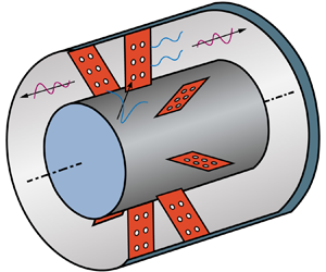
Consider an annular stator cascade of  $V$ vanes inside an infinite hard-walled duct with a uniform subsonic axial mean flow of inviscid perfect gas, as shown in figure 1. A cylindrical coordinate is taken, and the axial coordinate is denoted as $z$. Coordinates with superscript $'$ represent the coordinates of the source point, and the coordinates without $'$ are those of the observation point. The cascade is of hub radius $R_h$, tip radius $R_d$, and chord length $b$, with a background flow of axial velocity $U$ and no swirling flow. Porosity is applied to create soft boundaries on the vanes, and the stator vanes are assumed to be identical and evenly spaced zero-thickness perforated plates with zero stagger angle and no camber. The viscosity effects near the vanes are retained with the unsteady Kutta condition applied in the form of zero pressure jump at the trailing edge and an integrable pressure singularity at the leading edge. Incident waves could be either acoustic or vortical, assuming that the disturbances are small and isentropic. In this specific paper, however, we focus on the interaction noise with incident vortical disturbances. The trailing edge self-noise is neglected here.

Figure 1. Schematic of an annular perforated cascade.
The rotor–stator interaction noise can be divided into two kinds: one is the interaction between the viscous wake of the rotor and the solid boundaries of the stator; the other is induced by the potential field of the rotor interacting with the stator. However, the potential field usually decays quickly in a turbofan-engine fan stage, therefore the rotor–stator interaction noise is dominated by the interactions caused by the viscous wake (Peake & Parry Reference Peake and Parry2012). In rotor-fixed cylindrical coordinates, the viscous wake of the rotor can be separated into a steady flow component and an unsteady component. In the steady flow field, each rotor blade will induce a velocity deficit behind it, and an evenly distributed rotor cascade of  $B$ identical blades will create a velocity field with periodicity $2{\rm \pi} /B$ in the circumferential direction, as illustrated in figure 2. Subsequently, the steady component of the rotor wake can be expanded into a Fourier's series of $\varphi$ in the form
 \begin{equation} \sum_{s=0}^{\infty}W_s(r,z) \exp({\mathrm{i}sB\varphi}), \end{equation}
where  $W_s(r,z)$ are the Fourier coefficients, and $\varphi$ is the circumferential coordinate; $s$ is the order of the series. If we transform the velocity field to the stator-fixed coordinate system, then the $s$th-order component will become
 \begin{equation} W_s(r,z) \exp({\mathrm{i}sB(\varphi - \varOmega t)}), \end{equation}
where  $\varOmega$ is the angular rotation speed of the rotor. This corresponds to a fluctuating upwash velocity on vane surfaces at frequency $\omega _s = sB\varOmega$, which will correspondingly induce pressure loading on vanes at the same frequency. Accordingly, the $s=0$ part of the velocity Fourier series is responsible for the steady loading on stator vanes, while the other terms will interact with the stator cascade to create tonal noise at $s$ times the blade passing frequency. Hereafter, we consider the tonal interaction noise as an illustration of the noise reduction mechanism by perforations. As for the unsteady component of the rotor wake that is mostly related to the turbulences in the wake, it is responsible for the broadband rotor–stator interaction noise and might be investigated in future studies.
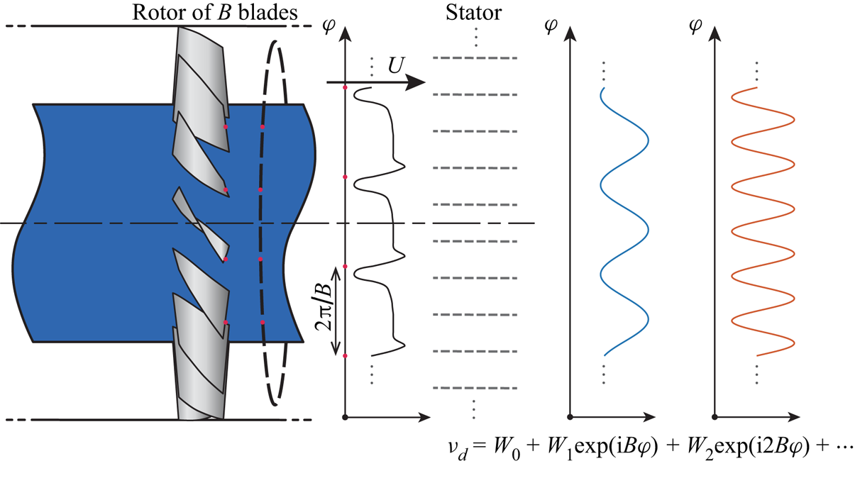
Figure 2. The steady component of the rotor wake velocity and its Fourier expansion over the circumferential direction. The Fourier components then interact with the stator cascade to produce tonal rotor–stator interaction noise.
2.1. Discussion on sound source terms
We derived our solution of the scattered field based on the generalized Lighthill's equation by Goldstein (Reference Goldstein1976, pp. 189–192), which extends Lighthill's acoustic analogy (Lighthill Reference Lighthill1952) to include the effects of solid boundaries using the generalized Green's formula (a generalization of the usual Green's formula to wave equations in a uniformly moving medium). We choose  $G$ to be the Green's function for the infinite rigid wall annular duct with a uniform subsonic axial background flow, satisfying the wave equation in a medium of uniform axial velocity $U$ and isentropic speed of sound denoted as $c_0$, i.e.
 \begin{equation} \nabla^2 G - \frac{1}{c_0^2}\,\frac{\mathrm{D}_0^2}{\mathrm{D}\tau^2}G ={-}\delta(t-\tau)\,\delta(\boldsymbol{x}-\boldsymbol{y}), \end{equation}
and a boundary condition of zero normal derivative at duct walls,
 \begin{equation} \left. \frac{\partial G}{\partial n} \right|_{\boldsymbol{x}\text{ at duct walls}} = 0 . \end{equation}
It is further required that  $G$ satisfies the causality condition
 \begin{equation} G=\frac{\mathrm{D}_0 }{\mathrm{D}\tau}G=0 \quad \text{for}\ t<\tau. \end{equation}
In our case, the material derivative is
 \begin{equation} \frac{\mathrm{D}_0}{\mathrm{D}\tau} \equiv \frac{\partial}{\partial\tau}+U\,\frac{\partial}{\partial z'}, \end{equation}
where  $t$ is the observation time, and $\tau$ is the time of source; $\boldsymbol {x},\boldsymbol {y}$ are respectively the spatial coordinate vectors of the observation point and the source point, and $z'$ is the axial coordinate in the source system.
In the cylindrical coordinate system illustrated in figure 1, the Green's function for a subsonic axial flow in a hard-walled annular duct can be expressed as (Sun & Wang Reference Sun and Wang2021, pp. 92–98)
 \begin{align} &G(r,\varphi,z,t\mid r',\varphi',z',\tau) =\frac{1}{4{\rm \pi}^2}\sum_{m={-}\infty}^{+\infty}\sum_{n=1}^{+\infty} \frac{\phi_m(k_{mn}r)\,\phi_m(k_{mn}r')}{2{\rm \pi}} \exp({\mathrm{i}m\varphi}) \exp({-\mathrm{i}m\varphi'}) \nonumber\\ &\quad \times \int_{-\infty}^{+\infty} \int_{-\infty}^{+\infty} \frac{\exp({\mathrm{i}\alpha(z-z')})}{\beta^2\alpha^2 + 2Mk_0\alpha-k_0^2+k_{mn}^2} \exp({-\mathrm{i}\omega(t-\tau)})\,\mathrm{d}\alpha\,\mathrm{d}\omega, \end{align}
where  $\phi _m(k_{mn}r)$ is the normalized radial eigenfunction of the hard-walled annular duct (see Sun & Wang Reference Sun and Wang2021, pp. 95–98) satisfying the orthogonality as
 \begin{equation} \int_{R_h}^{R_d}\phi_m(k_{mj}r)\,\phi_m(k_{ml}r)\,r\,\mathrm{d}r=\delta_{jl}, \end{equation}
and  $k_{mn}$ is the corresponding eigenvalue of the circumferential mode $m$ and radial mode $n$ (in our notation, $n=1,2,3,\ldots$). Accordingly, duct modes are denoted as $(m,n)$. Here, $M=U/c_0$ is the Mach number of the background flow, and $k_0=\omega /c_0$ is the wavenumber of sound; $\beta$ is taken to be the Prandtl–Glauert transformation factor as $\beta = \sqrt {1-M^2}$. By selecting this Green's function, the hard-walled duct modes will be included explicitly in the expression of the scattered pressure field, thus simplifying the following aeroacoustic analysis. The boundaries of the vanes are not included in the derivation of the Green's function, and will be considered later when establishing the integral equation using the singularity method.
We then ignore the insignificant quadrupole volume source term (Goldstein Reference Goldstein1976, pp. 220–222) in the generalized Lighthill's equation to obtain the scattered pressure field in the form
 \begin{equation}
p'(\boldsymbol{x},t)=\int_{{-}T}^T\int_{S(\tau)}
\frac{\partial G}{\partial y_i}\,f_i
\,\mathrm{d}S(\boldsymbol{y})\,\mathrm{d} \tau +
\int_{{-}T}^T\int_{S(\tau)}\rho_0V_n'\,\frac{\mathrm{D}_0
G}{\mathrm{D}\tau}\, \mathrm{d}
S(\boldsymbol{y})\,\mathrm{d} \tau,\quad T\rightarrow\infty
. \end{equation}
\begin{equation}
p'(\boldsymbol{x},t)=\int_{{-}T}^T\int_{S(\tau)}
\frac{\partial G}{\partial y_i}\,f_i
\,\mathrm{d}S(\boldsymbol{y})\,\mathrm{d} \tau +
\int_{{-}T}^T\int_{S(\tau)}\rho_0V_n'\,\frac{\mathrm{D}_0
G}{\mathrm{D}\tau}\, \mathrm{d}
S(\boldsymbol{y})\,\mathrm{d} \tau,\quad T\rightarrow\infty
. \end{equation}
The first integration term corresponds to the dipole sources, and the second integration term corresponds to the monopoles, as illustrated in 3(a). Here, vector  $f_i$ represents the surface force acting on the fluid by the boundaries, and $V_n'$ is the normal velocity of the boundary surfaces relative to the mean flow, with $\rho _0$ being the density of the background flow. Also, $\pm T$ are the upper and lower limits of the time integral, with $T$ taken to be infinity when Green's formula is used. Additionally, the surface integral $\int _{S(\tau )}(\,\cdot\,)\,\mathrm {d}S(\boldsymbol {y})$ needs to be performed only on the vane surfaces, since in a hard-walled duct, both terms at the duct surfaces can be eliminated due to the inviscid flow assumption, the selection of the Green's function and the impenetrable boundary condition at duct walls (Goldstein Reference Goldstein1976, pp. 192–195).

Figure 3. Illustration of (a) sources on the perforated plate and (b) the Rayleigh conductivity model.
With the  $s$th-order component of the rotor wake disturbance at frequency $\omega _s$ as the incident wave, the induced pressure jump across the vane can correspondingly be written as
 \begin{equation} {\rm \Delta} P_s\exp({-\mathrm{i}\omega_s \tau}) = (P_s^{(+)} - P_s^{(-)}) \exp({-\mathrm{i}\omega_s \tau}). \end{equation}
Here, we use the superscripts  $(\pm )$ to distinguish the two surfaces of the stator vane, and we define the upper side ( $+$) as the surface with the larger circumferential coordinate, and the lower side ( $-$) as the surface with the smaller circumferential coordinate. The only dominant source of the surface force $f_i^{(\pm )}$ is the pressure perturbation $P_s^{(\pm )}\exp ({-\mathrm {i}\omega _s \tau })$ on the upper side and the lower side of the vanes, because the shear stress is ignorable on the vane surfaces when the Reynolds numbers are high, as in practical aero-engines. The direction of the surface force $f_i^{(\pm )}$ then becomes normal to the vane surfaces. Unlike impermeable stator vanes on which $V_n'$ is restricted to be zero, on porous vanes the unsteady loading ${\rm \Delta} P_s$ further produces fluctuating volume fluxes through perforations. These unsteady fluxes lead to a non-zero $V_n'$ on both sides of the vane that may contribute to the monopole source term. However, under the assumption of zero-thickness vanes, the continuity across the apertures on the plate ensures that the normal velocities on the upper side ( $V_n'^{(+)}$) and the lower side ( $V_n'^{(-)}$) of the vanes are of the same absolute value but with opposite signs. Consequently, if $h$ is the thickness of the vane, then the monopoles distributed on the two sides will form dipole-like structures with negligible dipole strength ( $|V_n'^{(\pm )}|\,h$) of ${O}(h)$, since on each side the monopole strength $|V_n'^{(\pm )}|$ is finite, and the distance between the two poles goes to zero as $h\rightarrow 0$.
This indicates that for a thin-vane perforated cascade model with which we are concerned, the monopole source terms from the two sides of the vane are in opposite phase with the same magnitude, and will cancel each other out, with only the dipole-source-induced pressure fluctuations left in the far-field areas. Therefore, we can neglect the second term in (2.9) and deal with only the first term, i.e. the dipole source term. This is the same as in a hard-vane cascade fluid–structure interaction problem, and it greatly simplifies the expression for the scattered pressure field  $p'(\boldsymbol {x},t)$. The stator vanes can correspondingly be modelled as dipole distributions using the acoustic analogy, and be replaced by lifting surfaces similar to a hard-vane situation (Namba Reference Namba1987; Zhang et al. Reference Zhang, Wang, Jing, Liang and Sun2017), only with different boundary conditions on vanes. Again with the zero-thickness assumption, the integration of $f_i$ on the two sides leaves only the pressure difference ${\rm \Delta} P_s$ (Zhang et al. Reference Zhang, Wang, Jing, Liang and Sun2017). Consequently, the induced pressure field reduces to
 \begin{equation} p'(\boldsymbol{x},t)=\int_{{-}T}^T\int_{S(\tau)} \frac{\partial G}{\partial n'}\, {\rm \Delta} P_s(\boldsymbol{y})\exp({-\mathrm{i}\omega_s \tau})\,\mathrm{d}S(\boldsymbol{y})\,\mathrm{d} \tau, \quad T\rightarrow\infty, \end{equation}
where  ${\partial }/{\partial n'}$ represents the derivative normal to the vane surfaces, and the integration domain of the surface integral $\int _{S(\tau )}(\,\cdot \,)\,\mathrm {d}S(\boldsymbol {y})$ reduces to one plane at each vane's position instead of two planes at both the upper and lower sides. Additionally, in our model, where radially placed straight vanes are considered in a cylindrical coordinate system, the normal derivative ${\partial }/{\partial n'}$ is replaced by ${\partial }/{(r'\,\partial \varphi ')}$.
2.2. Boundary conditions
We have inherently applied a solid boundary condition on duct walls in the selection of the Green's function and a non-reflecting boundary condition on the upstream and downstream cross-sections by studying cascades in an infinite duct, as mentioned before. For the soft boundary vanes, we consider perforated plates with a rigid structure and evenly spaced circular apertures, which are modelled with the Rayleigh conductivity  $K_R$. The porosity on the plates allows fluctuating volume fluxes across the apertures, resulting in a space-averaged normal velocity $v_R=\tilde {v}_R \exp ({-\mathrm {i}\omega _s\tau })$ at the cascade vane surfaces, which is the physical velocity permitted by the soft boundary condition. The induced perturbation velocity normal to the vane surfaces is its circumferential component $v_\varphi ' = \tilde {v}'_\varphi \exp ({-\mathrm {i}\omega _s\tau })$ for the radially placed straight vanes that we studied. Let $v_d=\tilde {v}_d \exp ({-\mathrm {i}\omega _s\tau })$ denote the normal disturbance velocity of the incident waves. Then on the vane surfaces, the porous plate boundary condition should be satisfied in the form
 \begin{equation} {v}_R=v'_\varphi + v_d, \end{equation}
or, after dropping the time factor, as
 \begin{equation} \tilde{v}_R=\tilde{v}'_\varphi + \tilde{v}_d. \end{equation}
This boundary condition, along with the simplified generalized Lighthill's equation (2.11), is in principle sufficient to solve the problem with a given incident disturbance velocity  $v_d$ if $v_R$ and $v_\varphi '$ are both related to the unknown dipole source on vanes, namely the unsteady pressure loading ${\rm \Delta} P_s$. The detailed expression of $v_\varphi '$ will be derived in § 2.3, and the relation of ${v}_R$ to ${\rm \Delta} P_s$ is discussed as follows. Note that (2.13) reduces to the impermeable boundary condition of a hard vane when $\tilde {v}_R=0$.
For the rigid perforated vanes that we discussed, we first drop the fluctuating time factor  $\exp ({-\mathrm {i}\omega _s\tau })$. Then the relation between the induced volume flux $Q$ through a single orifice from the lower ( $-$) to the upper ( $+$) side, and the fluctuating pressure difference ${\rm \Delta} P_s$ across the vane, may be described with the definition of the Rayleigh conductivity (Howe Reference Howe1998, § 5.3.1)
 \begin{equation} K_R = \frac{\mathrm{i}\omega_s \rho_0 Q}{P_s^{(+)} - P_s^{(-)}}= \frac{\mathrm{i}\omega_s \rho_0 Q}{{\rm \Delta} P_s}, \end{equation}
as illustrated in figure 3(b). The Rayleigh conductivity is  $K_R = 2R$ for an ideal inviscid flow through circular apertures of radius $R$ on a zero-thickness plate, with no tangential or bias mean flow. In more general situations such as that with a mean background flow, however, $K_R$ is usually complex, and it is convenient to use its non-dimensionalized form
 \begin{equation} K_R = 2R(\varGamma_R(\omega)-\mathrm{i}\,\varDelta_R(\omega)), \end{equation}
where  $\varGamma _R(\omega )$ and $\varDelta _R(\omega )$ are real-valued functions of the frequency $\omega$, and $\varDelta _R(\omega )$ is related to the dissipation of the acoustic energy. Explicit expressions for $K_R$ are unattainable for porous plates with tangential background flow (Howe Reference Howe1998, pp. 371–375), therefore we use designated values of conductivity to study the effects of soft-vane cascades for simplicity and to focus on the essential mechanisms of the noise reduction by porosity.
On the other hand, in order to extend the concept of the Rayleigh conductivity to the entire perforated vane with multiple apertures, the short-range interactions between orifices should be negligible, and this could be achieved by setting the distance  $d$ between orifices much larger than the aperture radius $R$. For evenly spaced perforations, this is usually ensured by restricting the fractional open area $\alpha _H$ to be less than $0.04$ (Bendali et al. Reference Bendali, Fares, Piot and Tordeux2013). Another requirement to ensure a local reaction of the pressure jump is that the spacing $d$ should be less than half the sound wavelength $\lambda$ (Bendali et al. Reference Bendali, Fares, Piot and Tordeux2013), which is achievable with a small-radius aperture design. Additionally, the orifice radius $R$ should be small compared to the wavelength $\lambda$ such that the pressure difference ${\rm \Delta} P_s$ can be regarded as constant over the aperture. Note that in our case, where incident vortical disturbances are considered, the wavelength should be regarded as that of the scattered acoustic waves, i.e. $\lambda =2{\rm \pi} c_0/\omega _s$. With all the conditions satisfied, we may further average the volume fluxes $Q$ in (2.14) using the fractional open area $\alpha _H$ to smear them over the entire perforated plate surface, as was done in Hughes & Dowling (Reference Hughes and Dowling1990) and Baddoo & Ayton (Reference Baddoo and Ayton2020), and then obtain the fluctuating flow velocity normal to the vane surfaces as
 \begin{equation} \tilde{v}_R=\frac{\alpha_H}{{\rm \pi} R^2}\,Q =\frac{\alpha_H}{{\rm \pi} R^2}\, \frac{-\mathrm{i} K_R}{\omega_s\rho_0}\,{\rm \Delta} P_s, \end{equation}
since by continuity,  ${v}_R$ should be equal to the averaged flux velocity induced by the unsteady pressure difference.
By referring to the definition of the acoustic impedance  $p/v=z\rho _0 c_0$, we may further define an equivalent normalized impedance for the Rayleigh conductivity boundary condition with the fluctuation angular frequency $\omega _s$, expressed as
 \begin{equation} z_{{eqv}} = \frac{{\rm \Delta} P_s}{-\tilde{v}_R}\,\frac{1}{\rho_0 c_0} = \frac{-\mathrm{i}{\rm \pi} R\omega_s}{2\alpha_H (\varGamma_R(\omega_s) - \mathrm{i}\,\varDelta_R(\omega_s))c_0}. \end{equation}
2.3. Implementation of the lifting surface method
Hereafter, we assume that the incident disturbance has a circumferential periodicity and that its  $s$th-order component wave has $\sigma$ periods over one circle. (For the steady rotor wakes introduced before, we have $\sigma =sB$.) The resulting pressure loading on a cascade of $V$ identical evenly spaced vanes should consequently be in similar forms with a constant inter-blade phase angle difference ${2{\rm \pi} \sigma }/{V}$ between the vanes. Label the vanes from $1$ to $V$ as $\varphi '$ increases, and set ${\rm \Delta} P_s(r',z',\varphi ')\exp ({-\mathrm {i}\omega _s\tau })$ to be the unsteady loading distribution over the first vane. If the rotor is rotating in the positive direction of the circumferential coordinate, then the pressure jump on the $k$th stator vane would be
 \begin{equation} {\rm \Delta} P_s(r',z',\varphi')\exp\left({\mathrm{i}(k-1)\, \frac{2{\rm \pi}\sigma}{V}}\right)\exp({-\mathrm{i}\omega_s\tau}), \end{equation}
and the corresponding circumferential coordinate on the  $k$th vane is $\varphi ' + 2{\rm \pi} (k-1)/V$. Substituting the Green's function (2.7) into (2.11), and using the above periodicity of the unsteady loading on different vanes, we then have
 \begin{align} p'(\boldsymbol{x},t) &=
\frac{-\mathrm{i}}{8{\rm \pi}^3}\sum_{m={-}\infty}^{+\infty}
\sum_{n=1}^{+\infty}\phi_m(k_{mn}r)\exp({\mathrm{i}m\varphi})
\int_{S_1(\tau)}\sum_{k=1}^{V}\frac{m}{r'}
\phi_m(k_{mn}r')\exp({-\mathrm{i}m\varphi'}) \nonumber\\
&\quad
\times\exp\left({\mathrm{i}\,\frac{2{\rm \pi}}{V}\,(k-1)(\sigma-m)}\right)
\nonumber\\ &\quad \times{\rm \Delta} P_s(r',z',\varphi')
\int_{-\infty}^{+\infty} \exp({-\mathrm{i}\omega t})
\int_{-\infty}^{+\infty}
\frac{\exp({-\mathrm{i}\alpha(z-z')})}{\beta^2 +
2Mk_0\alpha - k_0^2+k_{mn}^2} \nonumber\\ &\quad
\times\int_{{-}T}^{T}
\exp({-\mathrm{i}\omega_s\tau})\exp({\mathrm{i}\omega
\tau})
\,\mathrm{d}\tau\,\mathrm{d}\alpha\,\mathrm{d}\omega\,\mathrm{d}S(\boldsymbol{y}),\quad
T\rightarrow\infty, \end{align}
\begin{align} p'(\boldsymbol{x},t) &=
\frac{-\mathrm{i}}{8{\rm \pi}^3}\sum_{m={-}\infty}^{+\infty}
\sum_{n=1}^{+\infty}\phi_m(k_{mn}r)\exp({\mathrm{i}m\varphi})
\int_{S_1(\tau)}\sum_{k=1}^{V}\frac{m}{r'}
\phi_m(k_{mn}r')\exp({-\mathrm{i}m\varphi'}) \nonumber\\
&\quad
\times\exp\left({\mathrm{i}\,\frac{2{\rm \pi}}{V}\,(k-1)(\sigma-m)}\right)
\nonumber\\ &\quad \times{\rm \Delta} P_s(r',z',\varphi')
\int_{-\infty}^{+\infty} \exp({-\mathrm{i}\omega t})
\int_{-\infty}^{+\infty}
\frac{\exp({-\mathrm{i}\alpha(z-z')})}{\beta^2 +
2Mk_0\alpha - k_0^2+k_{mn}^2} \nonumber\\ &\quad
\times\int_{{-}T}^{T}
\exp({-\mathrm{i}\omega_s\tau})\exp({\mathrm{i}\omega
\tau})
\,\mathrm{d}\tau\,\mathrm{d}\alpha\,\mathrm{d}\omega\,\mathrm{d}S(\boldsymbol{y}),\quad
T\rightarrow\infty, \end{align}
where the surface integral domain reduces to that of the first vane,  $S_1(\tau )$. From the relations
 \begin{equation} \left.\begin{gathered} \sum_{k=1}^{V}\exp\left[\mathrm{i}\,\frac{2{\rm \pi}}{V}\,(k-1)(\sigma-m)\right] =\left\{\begin{array}{ll} V, & m=\sigma-qV, \\ 0, & m\neq\sigma-qV, \end{array}\right. q=0,\pm1,\pm2,\ldots, \\ \lim_{T\rightarrow\infty}\int_{{-}T}^{T}\exp({-\mathrm{i}(\omega_s-\omega)\tau})\,\mathrm{d}\tau = 2{\rm \pi}\delta(\omega_s-\omega), \end{gathered}\right\} \end{equation}
and using the residue theorem for the infinite integration of the axial wave number  $\alpha$ with the causality condition applied, the scattered sound field is related to the unsteady loading ${\rm \Delta} P_s$ on the first ( $k=1$) vane by
 \begin{align} p'(\boldsymbol{x},t) &= \frac{V\exp({-\mathrm{i}\omega_s t})}{4{\rm \pi}} \sum_{q={-}\infty}^{+\infty}\sum_{n=1}^{+\infty}\phi_m(k_{mn}r) \nonumber\\ &\quad \times\exp({\mathrm{i}m\varphi}) \int_{S_1(\tau)}\frac{m}{\kappa_{nm}r'}\, \phi_m(k_{mn}r')\exp({-\mathrm{i}m\varphi'})\,{\rm \Delta} P_s(r',z',\varphi') \nonumber\\ &\quad \times \left\{ H(z-z')\exp({\mathrm{i}\alpha_1(z-z')}) \right. \nonumber\\ &\qquad \left.{}+H(z'-z)\exp({\mathrm{i}\alpha_2(z-z')})\right\} \mathrm{d}S(\boldsymbol{y}),\quad m=\sigma-qV. \end{align}
Here,  $\delta (\,\cdot \,)$ represents the Dirac delta function, and $\mathrm {H}(\,\cdot \,)$ denotes the Heaviside function.
In addition, the linearized circumferential inviscid momentum equation can be expressed as
 \begin{equation} \frac{\partial v_\varphi'}{\partial t}+U\,\frac{\partial v_\varphi'}{\partial z}={-}\frac{1}{\rho_0}\, \frac{\partial p'}{r\,\partial \varphi}, \end{equation}
where the circumferential perturbation velocity  $v_\varphi '$ induced by the lifting surfaces also has a time dependence $\exp ({-\mathrm {i}\omega _s t})$ such that ${\partial v_\varphi '}/{\partial t} = -\mathrm {i}\omega _s v_\varphi '$. We first substitute (2.19) into (2.22), then (2.22) reduces to a first-order ordinary differential equation that can be solved to obtain the induced upwash velocity
 \begin{align} v_\varphi'(\boldsymbol{x},t) &={-}\frac{V\exp({-\mathrm{i}\omega_s t})}{2{\rm \pi}\rho_0 U} \sum_{q={-}\infty}^{+\infty}\sum_{n=1}^{+\infty}\frac{m}{r}\,\phi_m(k_{mn}r) \exp({\mathrm{i}m\varphi}) \nonumber\\ &\quad \times \int_{S_1(\tau)}\frac{m}{r'}\,\phi_m(k_{mn}r') \exp({-\mathrm{i}m\varphi'})\,{\rm \Delta} P_s(r',z',\varphi') \nonumber\\ &\quad \times \left\{Q_1 \exp({\mathrm{i}\alpha_1(z-z')}) + Q_2\exp({\mathrm{i}\alpha_2(z-z')}) \right.\nonumber\\ &\qquad \left.{}+ Q_3 \exp({\mathrm{i}\alpha_3(z-z')})\right\} \mathrm{d}S(\boldsymbol{y}),\quad m=\sigma-qV, \end{align}
following procedures similar to those in the derivation of (2.21). The integration constant that occurs when solving (2.22) is taken to be zero, assuming that there is no disturbance velocity at positions far upstream (Namba Reference Namba1972). Here and above,
 \begin{gather} Q_1 = \frac{H(z-z')\,M\beta^2}{2\kappa_{nm}(M\kappa_{nm}-k_0)},\quad Q_2 ={-}\frac{H(z'-z)\,M\beta^2}{2\kappa_{nm}(M\kappa_{nm}+k_0)},\quad Q_3 = \frac{H(z-z')\,M^2}{k_0^2+M^2 k_{mn}^2}, \end{gather}
 \begin{gather}\alpha_1=\frac{-Mk_0+\kappa_{nm}}{\beta^2},\quad \alpha_2=\frac{-Mk_0-\kappa_{nm}}{\beta^2},\quad \alpha_3=\frac{\omega_s}{U}=\frac{k_0}{M}, \end{gather}
and
 \begin{equation} \kappa_{nm} = \left\{\begin{array}{ll} \sqrt{k_0^2-\beta^2k_{mn}^2}, & \mathrm{if}\ k_0^2 > \beta^2k_{mn}^2, \\ \mathrm{i}\sqrt{\beta^2k_{mn}^2-k_0^2}, & \mathrm{if}\ k_0^2<\beta^2k_{mn}^2. \end{array}\right. \end{equation}
The  $\exp ({\mathrm {i}\alpha _1(z-z')})$ and $\exp ({\mathrm {i}\alpha _2(z-z')})$ terms correspond to the upstream and downstream propagating pressure waves, and the $\exp ({\mathrm {i}\alpha _3(z-z')})$ term corresponds to the vortical waves convected downstream. The expressions for the scattered pressure field of the perforated cascade and its induced velocity, (2.21) and (2.23), are the same as in a hard-vane cascade lifting surface method (Zhang et al. Reference Zhang, Wang, Jing, Liang and Sun2017). This is because the source characteristics of a perforated cascade and a hard-vane cascade are also the same, with only dipoles distributed on the vane surfaces, as we have proved in § 2.1.
So far we have obtained the expressions for both  $v_R$ and $v'_\varphi$ with an unknown unsteady loading ${\rm \Delta} P_s \exp ({-\mathrm {i}\omega _s t})$. However, to solve numerically for ${\rm \Delta} P_s$, truncation of the infinite series for $m$ and $n$ in (2.23) is unavoidable, and the error of truncating $m$ is difficult to control due to the non-uniform convergence of the Fourier series (Namba Reference Namba1972). To better restrict the truncation errors and evaluate the singularities in the original equation, we apply the finite radial mode expansion method proposed by Namba (Reference Namba1972, Reference Namba1987) to approximate the original radial eigenfunctions with a limited set of $L$ functions $\psi _k^{(\infty )}(r)$:
 \begin{equation} \phi_m(k_{mn}r) \approx \sum_{k=1}^{L} {BB}_{n,k}^m\,\psi_k^{(\infty)}(r). \end{equation}
Detailed definitions and the corresponding applications of  $\psi _k^{(\infty )}(r)$ and the expansion coefficients ${BB}_{n,k}^m$ are shown in Appendix A, and the accuracy of this approximation can be improved to any level by simply increasing $L$ (Namba Reference Namba1972). Accordingly, after representing all the radial eigenfunctions with $\psi _k^{(\infty )}(r)$ and further separating the singular parts from the regular parts of the kernel function, (2.23) can be rewritten as
 \begin{equation} \tilde{v}'_\varphi = \int_{S_1(\tau)} {\rm \Delta} P_s(r',z',\varphi')\, K(r,r',z,z',\varphi,\varphi')\,\mathrm{d}S(\boldsymbol{y}), \end{equation}
where the final expression for the kernel function  $K$ is described in (A7)–(A10). Substituting (2.28) and (2.16) into the boundary condition (2.13), we obtain one integration equation that describes the relation between the unknown ${\rm \Delta} P_s$ and the input $\tilde {v}_d$. With a given distribution of the normal velocity induced by the incident wave, we are able to solve the unsteady pressure loading ${\rm \Delta} P_s$, and then obtain the scattered sound field $p'(\boldsymbol {x},t)$ using (2.21).
According to Morfey's definition of acoustic intensity in an irrotational uniform-entropy flow (Morfey Reference Morfey1971), the axial sound energy flux inside a background flow of axial velocity  $U$ could be formulated as
 \begin{equation} I_z=\langle p'u_z \rangle + \frac{U}{\rho_0 c_0^2}\,\langle p'^2\rangle + \frac{U^2}{c_0^2}\,\langle p'u_z\rangle + \rho_0\,U\langle u_z^2\rangle, \end{equation}
where  $u_z$ is the axial component of the perturbation velocity, which can be solved by resorting to the momentum equation along with (2.21), and $\langle \,\cdot\, \rangle$ denotes the time average over one period. Integrating $I_z$ over the annular-duct cross-section, we obtain the sound energy power propagating downstream ( $W_+$) and upstream ( $W_-$) for a cut-on mode $(m,n)$ as
 \begin{equation} W_\pm = \frac{{\rm \pi}\,|P_{mn}^\pm|^2}{\rho_0c_0}\,\frac{(1-M^2)^2 k_0\kappa_{nm}}{({\mp} k_0+M\kappa_{nm})^2}. \end{equation}
For cut-off modes, there is no axial acoustic energy flux. With the solution of the unsteady loading  ${\rm \Delta} P_s$, the cut-on sound mode coefficients $P_{mn}^\pm$ can be calculated from (2.21) for observation points at axial positions downstream and upstream of the cascade. Further averaging the sound power over the cross-section, we obtain the mean acoustic intensity $\bar {I}_{\pm }={W_\pm }/{{\rm \pi} (R_d^2-R_h^2)}$ and the corresponding sound power level (SPL) as
 \begin{equation} L_{I,\pm}=10\log({\bar{I}_{{\pm}}}/{I_0}),\quad I_0={10}^{{-}12}\,{\rm W}\,{\rm m}^{{-}2}. \end{equation}
3. Numerical solution with soft boundary conditions
With all the analytic expressions above, the integral equation (2.13) still needs to be solved numerically to obtain practical solutions. For radially placed straight vanes with zero swept or leaned angle, we may simply set the circumferential coordinate on the first vane as  $\varphi '=0$, and the unsteady loading distribution will degenerate to a function of just radial and axial coordinates, denoted as ${\rm \Delta} P_s(r',z')$. We then expand ${\rm \Delta} P_s$ using the finite radial basis functions $\psi _l^{(\infty )}(r)$ as
 \begin{equation} {\rm \Delta} P_s(r',z')=\sum_{j'=1}^{J} \psi_{j'}^{(\infty)}(r') \left[ A_{1j'} \cot\left(\frac{\xi'}{2}\right) + \sum_{i'=2}^{I}A_{i'j'}\sin((i'-1)\xi') \right], \end{equation}
with  $I$ axial terms and $J$ radial terms. As is usual, $J$ is taken to be the same as $L$, and the infinite series for $n$ in the kernel function is also truncated at $L$ terms. The Kutta condition is applied inherently here, with Glauert's transformation made to the axial coordinates for both the source position $z'$ and the observation location $z$, as is usual in a thin aerofoil theory, i.e.
 \begin{equation} z'=\frac{b}{2}\,(1-\cos\xi'),\quad z=\frac{b}{2}\,(1-\cos\xi),\quad z',z\in[0,b],\enspace \xi',\xi\in[0,{\rm \pi}]. \end{equation}
Substituting (3.1) into (2.28), the integration with respect to the radial coordinate  $r'$ could be performed analytically using the orthogonality of $\psi _l^{(\infty )}(r)$ (Namba Reference Namba1987), with only the axial coordinate left in the surface integration to be integrated numerically.
Applying a collocation method to solve for the integral equation (2.13), we choose  $I \times J$ evenly spaced control points on the vane at coordinates $(\xi _i,r_j),\ i=1,\ldots,I,\ j=1,\ldots,J$, and the incident wave disturbance velocities at these positions are denoted as $\boldsymbol {v}_{d,ij}$. With axial evenly spaced discrete source points similar to those in Whitehead (Reference Whitehead1962), we could then perform numerical integration in the $\xi '$ domain using the trapezoidal rule to finally obtain the discrete form of (2.28) as
 \begin{equation} \boldsymbol{\mathsf{M}}_{ij,i'j'}\boldsymbol{A}_{i'j'}=\tilde{\boldsymbol{v}}'_{\varphi,ij} . \end{equation}
Note that to calculate the Cauchy principal value of the integration of the singular kernel function  $K$, the control points must be placed at the middle of two source points. Therefore, the axial coordinates for the control points $\xi$ and the source points $\xi '$ are selected as
 \begin{equation} \xi_i=\frac{(2i-1){\rm \pi}}{2I},\quad \xi'_i=\frac{(i'-1){\rm \pi}}{I'},\quad i=1,\ldots,I,\enspace i'=1,\ldots,I'+1, \end{equation}
where  $I' = (2\eta +1) I$, and $\eta =3$. Here, $\eta$ is an adjustable integer coefficient. With an $\eta$ greater than 1, the source points are denser than the control points such that the surface integration can be calculated with higher accuracy without increasing the number of control points.
We then replace  ${\rm \Delta} P_s$ in (2.16) with the expansion (3.1). Due to the local reaction of the pressure fluctuations, it is simple to express the soft-wall averaged fluctuating velocity $\tilde {v}_R$ at the discrete control points $(\xi _i,r_j)$ in a matrix form as
 \begin{equation} \boldsymbol{\mathsf{M}}_{ij,i'j'}^R\boldsymbol{A}_{i'j'}=\tilde{\boldsymbol{v}}_{R,ij}, \end{equation}
where the coefficient matrix  $\boldsymbol{\mathsf{M}}_{ij,i'j'}^R$ is related to the local perforation properties $\alpha _H$, $R$ and $K_R$. This additional matrix $\boldsymbol{\mathsf{M}}_{ij,i'j'}^R$ is the key difference between the solution of a perforated cascade and a hard-vane cascade. In our case, where the soft boundary on vanes is reacting locally to the pressure fluctuations, the expansion (3.1) turns out to be very convenient for the construction of this coefficient matrix.
Finally, we substitute (3.3) and (3.5) into (2.13) and rearrange to construct a system of linear equations with the coefficient vector  $\boldsymbol {A}_{i'j'}$ as the unknown and the incident disturbance velocity vector $\tilde {\boldsymbol {v}}_{d,ij}$ as the right-hand side, in the form
 \begin{equation} (\boldsymbol{\mathsf{M}}_{ij,i'j'} - \boldsymbol{\mathsf{M}}_{ij,i'j'}^R)\boldsymbol{A}_{i'j'}={-}\tilde{\boldsymbol{v}}_{d,ij} . \end{equation}
By solving this linear system, we can obtain the unsteady loading distribution on vanes for any given incident wave, and from  ${\rm \Delta} P_s(r',z')$, we can further estimate the scattered sound field and its propagating acoustic energy.
It should be noted that in the above procedures, the boundary condition of the soft-vane cascade could be replaced by different kinds of conditions with minimum effort, such as those discussed in Baddoo & Ayton (Reference Baddoo and Ayton2020), provided that the pressure fluctuation is reacting locally with the soft vanes and that an explicit form of the relation  $\tilde {v}_R = f({\rm \Delta} P_s)$ is obtainable. Additionally, our method is not limited to uniform boundary conditions over the entire plate, as we can take the locally averaged value of the porosity parameter ${\alpha _H K_R}/{({\rm \pi} R^2)}$ (also used in Ayton et al. Reference Ayton, Colbrook, Geyer, Chaitanya and Sarradj2021) at each control point. That enables us to investigate the effects of partially perforated plates or uneven distributions of porosity on vanes, as long as all vanes in the cascade are of identical porosity distribution.
4. Validations
To validate our method, we compare our solutions with the results from two special cases: the 3-D hard-vane lifting surface model and the 2-D perforated cascade model.
4.1. Comparison with the 3-D hard-vane model
First, we set the Rayleigh conductivity  $K_R$ to be zero, and our model degenerates to a hard-vane annular cascade. Comparison is made between our solutions and the results from the benchmark problem of the third computational aeroacoustics workshop (Namba & Schulten Reference Namba and Schulten2000). The duct geometry parameters are $R_h=0.5\,\mathrm {m}$, $R_d=1.0\,\mathrm {m}$ and $b=2{\rm \pi} R_d /V$ in our dimensional model, with the rotor blade number $B=16$ and the stator vane number $V=24$. As shown at the beginning of § 2, this corresponds to a circumferential periodicity number $\sigma = sB$ and a disturbance frequency $\omega _s=sB\varOmega$ on the stator for the $s$th-order component of the rotor wake, where $\varOmega$ is the angular velocity of rotor rotation.
Accordingly, the incident vortical wave is defined as
 \begin{equation} v_d(r,\varphi,z,t) = w_s \exp\left({\mathrm{i} sB\left[\frac{\varOmega z}{U}+ \varphi-\theta(r)-\varOmega t\right]}\right),\quad \theta(r)={-}\frac{2{\rm \pi} q}{B}\left[ \frac{r-R_h}{R_d-R_h}\right], \end{equation}
where  $\theta (r)$ is the radial dependence function with an arbitrary real-valued wake-periodicity or wake-obliquity parameter $q$, and the wake velocity amplitude is given as a constant along the radial direction with $w_s=0.1U$. A positive $q$ represents that the wake at the stator root is ahead of that at the tip, as in typical fan designs. Results are obtained for the first-order vortical wave ( $s=1$), and the spanwise non-dimensional unsteady loading distributions ${\rm \Delta} C_p={{\rm \Delta} P_s(r')}/{(0.5\rho _0 U^2)}$ at different chord positions $z'/b$ are compared, as illustrated in figure 4. Radial wake periodicity parameter $q$ is set to be $q=3$, which corresponds to an average of 3 wakes intersecting each stator vane at the leading edge. The background flow Mach number is $M=0.5$, the sound speed is $c_0=340.0\,{\rm m}\,{\rm s}^{-1}$, the flow density is $\rho _0 = 1.225\,{\rm kg}\,{\rm m}^{-3}$, and the rotor tip Mach number is set to be $M_t = {\varOmega R_d}/{c_0}=0.783$, which correspondingly decides the shaft speed $\varOmega$.

Figure 4. Comparison of the unsteady loading at different axial positions for the  $q=3$ case with the results in the benchmark problem (Namba & Schulten Reference Namba and Schulten2000). The non-dimensional loading is taken as ${\rm \Delta} C_p={{\rm \Delta} P_s(r')}/{(0.5\rho _0 U^2)}$, and the leading edge position of the vane is set to be $z'=0$.
For axial positions close to the leading edge, our results agree well with both hard-vane lifting surface methods. At the positions further downstream, minor differences arise as the absolute value of the unsteady loading decreases, but overall our method matches well with the benchmark results.
We then solved for a porous 3-D annular cascade to demonstrate the convergence of our collocation method, and the results are shown in figure 5. As the number of the collocation control points  $I \times J$ increases, the propagating sound power approaches a final value, and the variation between each case decreases rapidly. By increasing the number of the collocation points, our result should converge to the physical solution of the problem.

Figure 5. Convergence of the calculated propagating sound power  $W_\pm$ with increasing control points for a perforated cascade.
4.2. Comparison with the 2-D soft-vane model
Now we compare our results with the 2-D perforated cascade model of uniform porosity exploiting the Wiener–Hopf method (Baddoo & Ayton Reference Baddoo and Ayton2020). Using zero stager angle as input, we calculate 2-D results with Baddoo's code published online at https://github.com/baddoo/complex-cascade-scattering, and with the hub–tip ratio set to be 0.99, our annular cascade model approximates a quasi-2-D situation. The non-dimensional parameter  $C_{II}$ of the case $II$ boundary condition in the 2-D model (Baddoo & Ayton Reference Baddoo and Ayton2020) corresponds to $-{2\mathrm {i} U\alpha _H K_R}/{{\rm \pi} R^2 \omega _s}$ in our 3-D method. Results with different porosity parameters $C_{II}$ are compared in figures 6 and figure 7. With an inter-vane phase difference angle $3{\rm \pi} /4$ in the 2-D model, we correspondingly choose the blade numbers to be $B=18$ and $V=48$ in our 3-D solution, and solve for the first-order vortical wave incidence as in (4.1a,b) with $s=1$ and $q=0$, where other input parameters are
 \begin{equation} \left.\begin{gathered} R_h=0.99\,\mathrm{m},\quad R_d=1.0\,\mathrm{m},\quad b=0.21708\,\mathrm{m},\quad M=0.3,\\ c_0 = 340.0\,{\rm m}\,{\rm s}^{{-}1}\quad \text{and}\quad \rho_0 = 1.225\,{\rm kg}\,{\rm m}^{{-}3}. \end{gathered}\right\} \end{equation}
The disturbance frequency is  $\omega _s b /2U \in (0,30]$, and the incident vortical wave amplitude is $w_1=0.1U$ for both cases. Solutions from the 2-D model and our 3-D method show good agreement, with only slight differences in the magnitudes of the downstream propagating acoustic energy.

Figure 6. Comparison of the unsteady lift coefficient  $C_L={\int _{0}^{b}{\rm \Delta} P_s(z')\,\mathrm {d}z'}/{({\rm \pi} b \rho _0 U w_1 )}$ with varying porosity and frequency. Solutions of the 2-D model (Baddoo & Ayton Reference Baddoo and Ayton2020) are illustrated by the dashed lines, and results of the present 3-D model are represented by the solid lines.

Figure 7. Comparison of the non-dimensionalised sound power propagating downstream for (a) the first and (b) the second acoustic mode with varying porosity and frequency, which corresponds to figure 11 in Baddoo & Ayton (Reference Baddoo and Ayton2020). In the 3-D model, the acoustic modes correspond to annular duct modes  $(18,1)$ and $(-30,1)$, and the acoustic power defined in (2.30) is non-dimensionalized by dividing $\rho _0 w_1^2U{\rm \pi} (R_d^2-R_h^2)/2$.
5. Results
In the following subsections, we investigate the solutions of a pressure-free gust impinging on a porous cascade, which corresponds to a rotor–stator interaction set-up, and evaluate the resulting propagating noise. We restrict our study to the first-order incident vortical wave as defined in (4.1a,b) with  $s=1$, and choose the same geometry set-ups as in § 4.1, with hub–tip ratio 0.5, blade numbers $B=16$, $V=24$, and other input parameters
 \begin{equation} \left.\begin{gathered} M=0.5,\quad c_0=340.0\,{\rm m}\,{\rm s}^{{-}1},\quad \rho_0 = 1.225\,{\rm kg}\,{\rm m}^{{-}3},\\ M_t=0.783\quad \text{and}\quad w_1 = 0.1U. \end{gathered}\right\} \end{equation}
5.1. Cascade response with uniform porosity on vanes
In this subsection, we study stator vanes with uniform perforations. To illustrate the effects of porosity, we select the aperture parameters common in practice as  $R=0.001\,\mathrm {m}$ and $\alpha _H = 0.02$, and set the real part of the conductivity $\varGamma _R$ to be zero. The imaginary part of the Rayleigh conductivity $\varDelta _R$ corresponds to both the permeability and the acoustic energy dissipation effect of the small apertures on plates (Howe Reference Howe1998, pp. 360–361), thus being able to provide a general view of porosity's influence over a hard-vane situation. Porosity here is assumed to be uniform over the entire vane, and the total sound power levels of the upstream and downstream cut-on modes are calculated with varying $\varDelta _R$ or $q$. For the first-order wake as $s=1$ and $\omega _s=B\varOmega$, there are two cut-on modes, being $(-8,1)$ and $(-8,2)$, respectively, and sound energy is summed for the two modes before calculating $L_{I,\pm }$. As shown in figure 8, for all three situations with different wake obliquity parameter $q$, both the upstream and downstream noise levels decrease as porosity increases, and a considerable noise reduction above 6 dB is achieved with a modest porosity at $\varDelta _R=1.0$. This conductivity value corresponds to a non-dimensional coefficient (see Baddoo & Ayton Reference Baddoo and Ayton2020)
 \begin{equation} C_{II}={-}\frac{2\mathrm{i} U\alpha_H K_R}{{\rm \pi} R^2 \omega_s} \approx 0.1016, \end{equation}
or the equivalent normalized impedance that we defined earlier in (2.17) as
 \begin{equation} z_{{eqv}} = \frac{{\rm \Delta} P_s}{-\tilde{v}_R}\,\frac{1}{\rho_0 c_0} \approx 0.9839, \end{equation}
which should be a rather achievable porosity in practical usage.

Figure 8. Propagating sound power levels for tilted ( $q=3$, $q=1.5$) and radially uniform ( $q=0$) incident wakes at different Rayleigh conductivities $\varDelta _R$, with constant $\varGamma _R=0$. We choose the first-order vortical wake incidence and the $M_t = 0.783$ set-up as in the benchmark problem (Namba & Schulten Reference Namba and Schulten2000).
Further illustration of the sound power level for varying wake obliquity with and without porosity is shown in figure 9. It is shown that the tilted incident wake leads to lower rotor–stator interaction noise for porous cascades in a way similar to a hard-vane cascade case, or it may be equally interpreted as porosity being effective in noise reduction for all obliquity parameter  $q$. Moreover, an interesting result occurs in the upstream noise power level where local minima exist. Whilst reducing propagating noise, the soft boundary condition seems to rescale the curves towards $q=0$ such that the positions of the local minima of the sound power level move to a smaller $|q|$.

Figure 9. Comparison of sound power levels propagating upstream and downstream at different wake obliquity parameters  $q$. The hard-vane situation and the $\varDelta _R=1.0$ case are shown, with the first-order vortical wake incidence and the $M_t = 0.783$ set-up as in the benchmark problem (Namba & Schulten Reference Namba and Schulten2000).
With the discussions on the source terms in § 2.1, we have clearly identified that for thin perforated vanes, the dipole source is still the dominant term in rotor–stator interaction noise. In our method, where porous vanes are modelled as lifting surfaces distributed with dipole sources, it is a direct deduction that porosity affects the scattered sound wave by altering the pressure jump over the vane surfaces, and that the acoustic modes in hard-walled duct sections are not influenced by the complex boundary conditions on the cascade vanes. This agrees with the conclusions in the 2-D model by Baddoo & Ayton (Reference Baddoo and Ayton2020), and the key factor of noise generation turns out to be the unsteady pressure loading on the vanes in both the 2-D and 3-D models.
Here, we may propose two principal mechanisms by which porosity affects the unsteady loading distribution on vanes and ultimately the propagating noise in a 3-D annular cascade. The first mechanism is that the permeability allowing normal velocity  $v_R$ across vane directly dampens the resulting unsteady loading ${\rm \Delta} P_s$ induced by the incident disturbance velocity $v_d$. The second mechanism is that the porosity also reduces the interactions among the unsteady loading at different positions and on different vanes, thus attenuating the 3-D coupling among the dipole sources ${\rm \Delta} P_s$ across the entire vane. These interactions among dipole sources are transmitted by the acoustic and vortical waves as shown by the kernel function in (A7), with the pressure wave part $K_{2}$ influencing $v_\varphi '$ in the upstream areas, and the pressure wave part $K_1$ along with the vortical wave part $K_3$ influencing $v_\varphi '$ in the downstream areas. Consequently, no place on the vanes is reacting locally to the incident perturbation velocity $v_d$, and the final distribution of the unsteady loading is strongly coupled.
5.1.1. Attenuation of pressure loading reacting to incident disturbances
Considering a simplified situation where both  $v_\varphi '$ and $\tilde {v}_R$ are dependent on the local pressure jump ${\rm \Delta} P_s$, a brief interpretation of the first mechanism can be obtained using the soft boundary normal velocity relation (2.13) as illustrated in figure 10. For hard vanes, the incident velocity $\tilde {v}_d$ must be fully offset by the dipole-source acoustic velocity $\tilde {v}'_\varphi$ to maintain the no-flux boundary condition, inducing a pressure jump ${\rm \Delta} P_s$ across the plate. For perforated vanes, however, the permeability of the perforations described by the Rayleigh conductivity $K_R$ allows the existence of a normal velocity $\tilde {v}_R$ that is proportional to ${\rm \Delta} P_s$. The argument difference between the complex velocity values $\tilde {v}'_\varphi$ and $-\tilde {v}_R$, which is caused by the time lag described in the Rayleigh conductivity, is less than $90^{\circ }$ with a positive $\varDelta _R$. Under such a case, the magnitude of $\tilde {v}'_\varphi$ and consequently the amplitude of ${\rm \Delta} P_s$ is lessened by the existence of porosity-related velocity $-\tilde {v}_R$.

Figure 10. Sketch of the effect of porosity on the resulting pressure loading in a simplified locally reacting model. Both the amplitude and phase of the unsteady loading  ${\rm \Delta} P_s$ are changed from the hard-vane situation depending on the argument and magnitude of the Rayleigh conductivity $K_R$, as $\tilde {v}_R\propto -\mathrm {i} K_R\, {\rm \Delta} P_s$.
For the previous results where  $\varDelta _R>0$ and $\varGamma _R=0$, $\mathrm {arg}(K_R)$ equals $-{\rm \pi} /2$ and the soft-vane boundary condition further becomes $|\tilde {v}_d| = |\tilde {v}_R| + |\tilde {v}'_\varphi |$ since $-\tilde {v}_R$ and $\tilde {v}'_\varphi$ are in the same orientation, as illustrated in figure 3(a). Consequently, with porosity on vanes, the incident normal velocity could be balanced by an unsteady loading of much smaller magnitude, which produces a lower noise level. If we assume further that $v_\varphi '$ is also in linear proportion to ${\rm \Delta} P_s$, then we may obtain a relation between the resulting pressure jump amplitude and the porosity strength as ${\rm \Delta} P_s \propto 1/(K_R+c)$ with a constant $c$. This leads to a $-{\log (K_R+c)}$ kind of decrease of SPL with increasing $\varDelta _R$, and a similar trend is observed in figure 8, showing that as $\varDelta _R$ increases, less noise power level reduction is achieved with the same $\varDelta _R$ increment. In a real 3-D annular cascade situation, however, complex interactions exist among the unsteady loading at different radial positions. In addition, the restriction of the Kutta condition will further complicate the relations between the resulting pressure jump distribution ${\rm \Delta} P_s$ and the conductivity of the porosity. Therefore, the above discussions could be treated only as a qualitative analysis. As illustrated in figure 11, on a 3-D annular cascade, the porosity dampens the absolute magnitude as well as the spanwise variation of the lift coefficient for both radially tilted ( $q=1.5$, $q=3.0$) and uniform ( $q=0$) wakes. The most profound effect is in the $q=1.5$ case, where both the absolute value and the spanwise variation of the lift coefficient are the largest. This indicates that porosity does reduce the amplitude of the unsteady loading ${\rm \Delta} P_s$, and shows that the soft boundary can further affect the radial distribution of ${\rm \Delta} P_s$.

Figure 11. Spanwise distribution of the unsteady lift coefficient  $|C_L(r')|$, where the lift coefficient for the 3-D cascade vane is defined as $C_L(r')={\int _{0}^{b}{\rm \Delta} P_s(r',z')\,\mathrm {d}z'}/{({\rm \pi} b \rho _0 U w_1 )}$. Solid lines illustrate $C_L$ distributions for hard-vane cases, whilst dashed lines represent the results for porous soft-vane cascades.
5.1.2. Attenuation of 3-D interactions among different positions
The second mechanism that attenuates the 3-D interactions is accomplished by permeability in a way similar to the previous mechanism, since the excessive pressure jump reacting to the normal velocity induced by the dipole sources elsewhere should be dampened simultaneously by the porosity. With conductivity  $\varDelta _R=1.0$, $\varGamma _R=0$ and incident wake $q=3$, the unsteady loading distributions ${\rm \Delta} P_s(r',z')$ for hard-vane and fully perforated cascades are compared in figure 12 for further insight into this mechanism.

Figure 12. Comparison of the amplitude distribution of the unsteady loading  ${\rm \Delta} P_s$ on (a) the hard vane and (b) the fully perforated vane; and the phase distribution of the unsteady loading ${\rm \Delta} P_s$ on (c) the hard vane and (d) the fully perforated vane, for $q=3$. Here, ${\rm \Delta} P_s$ is non-dimensionalized by $\rho _0 U^2 /2$, and the phase angle is restricted to $(-{\rm \pi},{\rm \pi} ]$.
With the implementation of the unsteady Kutta condition, there is usually a large-amplitude area for the unsteady loading near the leading edge. The unsteady pressure loading  $\Delta P_s$ in this area is a major source for propagating noise, and it also significantly influences the downstream loading distribution through the pressure and vortical waves corresponding to the $K_1$ and $K_3$ parts of the kernel function in (2.28), due to its dominant magnitude. Another consequence of its large amplitude is that there exist strong interactions within this area. As we may see in figures 12(a,c), for an incident wake with a radially uniform amplitude but a varying phase, the phase pattern of the reacting pressure loading ${\rm \Delta} P_s$ on the hard vanes almost immediately deviates from that of the incident wake velocity, which is illustrated in figure 13(a). Besides, the pressure amplitudes at different radial positions also decrease with various gradients from the leading edge to further downstream, forming a highly non-uniform radial distribution that can also be seen in figure 11. This is incompatible with a radially local reaction pressure pattern that can be calculated by a strip theory, as the strength of the incident wake is radially identical. All these phenomena should be greatly attributed to the interactions between different radial positions, which are fully 3-D.

Figure 13. Phase distributions of (a) the incident wake normal velocity  $\tilde {v}_d$ and (b) the unsteady loading ${\rm \Delta} P_s$, on a fully perforated vane with $\alpha _H=0.1$ in the $q=3$ case. The phase angle is restricted to $(-{\rm \pi},{\rm \pi} ]$.
However, with the porosity dampening these interactions, we observe a dramatic change in the phase and amplitude pattern of the unsteady loading in figures 12(b) and 12(d). The pressure phase is more organized, with a distribution similar to that of the incident wake over the entire leading half-plane. The phase distribution result of a more perforated case with  $\alpha _H=0.1$ (i.e. five times the original fractional open area) is given in figure 13(b), and the distribution is almost identical to that of the incident velocity in figure 13(a). Besides, the pressure amplitude is also more uniform in the radial orientation with porosity applied, and forms a more comparable axial decrease, eliminating the two amplitude minima near the leading edge in the hard-vane case. Accordingly, we may conclude that one major consequence of the second mechanism, which reduces the 3-D interactions between the dipole sources at different radial positions, is that the final distribution of ${\rm \Delta} P_s$ will be more dominated by a pressure loading reacting locally to the incident disturbance. A rather uniform amplitude distribution of ${\rm \Delta} P_s$ caused by a constant-amplitude incident wake, combined with a phase variation along the radial direction introduced by a wake obliquity having $q$ nodes from hub to tip, can greatly reduce the propagating noise induced by the entire cascade because the spanwise phase variation of the unsteady loading scatters sound energy into high-order radial modes that are cut-off, leading to less propagating acoustic energy (Namba Reference Namba1977). In other words, it creates more intervention between dipole sources at different radial positions, which diminishes the propagating acoustic energy by the cut-off mechanism. Not only could this effect directly decrease the propagating noise power by reducing the sound energy radiation from the large-amplitude area near the leading edge, it also attenuates the influence from this area to the downstream areas, and further reduces the excessive unsteady pressure loading at the trailing half-plane caused by its coupling with the leading edge large-amplitude area. An obvious result, which is shown in figure 12, is that the amplitude peak around the mid-chord and mid-span position is considerably attenuated by the implementation of porosity. In a modern turbofan aero-engine fan stage, the rotor wake is usually highly skewed such that the radial phase variation of the incident vortical wave is large. From what we have observed, with porosity applied, the 3-D interactions between different radial positions can be dampened to create a stronger phase variation in the unsteady loading on the stator vanes. This may further help with the rotor–stator interaction noise reduction.
We should emphasize that the two mechanisms discussed above are inherently coupled, as the porosity dampens the unsteady loading responding to the incident disturbance and to the interactions among the dipole sources at the same time. During the solution process, the two mechanisms are inseparable, and it is for the convenience of analysis that we discuss these two mechanisms separately. It is also noted that although the coupling of the unsteady loading response across the vanes is dampened by the porosity, the 3-D interactions among the perforated cascade still exist, such that our model is not equal to a quasi-3-D strip theory description.
Similar mechanisms are discovered in the study of permeable surfaces on an aerofoil (Teruna et al. Reference Teruna, Manegar, Avallone, Ragni, Casalino and Carolus2020) created by the porous material insertion, where the reduced source intensity and the destructive interference between sound sources at different positions induced by permeability are proposed to be responsible for the noise reduction of broadband trailing edge noise. On the other hand, as illustrated in figure 12, the amplitude reduction of the unsteady loading  ${\rm \Delta} P_s$ for a perforated cascade is basically non-uniform in the radial direction, even though the porosity is distributed uniformly. This indicates that for tilted incident wakes, the decrease of the unsteady pressure loading on a perforated vane, and ultimately the alteration of the propagating rotor–stator interaction noise, can be more attributed to the reduction of the interactions across different radial positions in a 3-D annular cascade.
5.2. Cascade response with non-uniform porosity on vanes
The fully porous design may induce a significant aerodynamic penalty for a stator cascade with great loss in efficiency, and a partially porous design could be the solution by which the impact of the porosity on the steady aerodynamic performance can be alleviated. In addition, there may also be structural limitations that restrict the application of porosity over the entire vane in practical situations. Therefore, as illustrated in figure 14, here we investigate two sets of porosity distribution, and only half of the vane is applied with the same porosity as previously discussed, which is  $R=0.001\,\mathrm {m}$, $\alpha _H = 0.02$ with conductivity $\varDelta _R=1.0$ and $\varGamma _R=0$. The first set varies the perforations along the axial position, where the porosity distributed at the upstream half plane is defined as case C, at the mid-chord half-plane as case D, and at the downstream half-plane as case E. Two additional cases with linear varying porosity ( $\alpha _H$) along axial positions are further investigated, in which the largest $\alpha _H$ is set to be $0.02$ such that the averaged fractional open area is the same as other partially perforated cases. Correspondingly, the porosity is axially decreasing in case F and increasing in case G. The second set varies the porous part along the radial position, where the porosity distributed at the tip half-span is defined as case F, at the mid-span half-plane as case G, and at the hub half-span as case H. For comparison, cases A and B correspond to a hard-vane cascade and a fully porous situation, respectively. The noise reduction effects of these cases are calculated for two different wake obliquity parameters $q=0$ and $q=3$, and the propagating noise power level results are summarized in tables 1 and 2. These serve as a preliminary qualitative discussion on the potential effects of non-uniform application of perforations, and more practical results concerning the authentic flow field in a real aero-engine may be discovered in future studies.

Figure 14. Illustration of the porosity distribution set-up from case C to case H.
Table 1. Noise reduction for different radially non-uniform porosity distributions.

Table 2. Noise reduction for different axially non-uniform porosity distributions.

In general, noise reduction can be achieved with partially perforated designs, but their SPL decrease is not as prominent as a fully porous design. For different axial distributions, porosity is most effective in the upstream half-plane as there exists a previously discussed large-amplitude area for the unsteady loading, and dampening the pressure jump in this area can further affect the downstream loading through 3-D interactions. For case C, both upstream and downstream propagating noise is greatly attenuated, and the pressure jump distribution results with a tilted incident wake ( $q=3$) are shown in figure 15. On the upstream half-vane, the amplitude of the unsteady loading is radially more uniform compared to the hard-vane result of case A in figure 12(a), and the phase distribution is also similar to that of the incident wake, as we might expect from the two aforementioned mechanisms. The porosity is not applied on the downstream half-vane, thus the pressure amplitude is less attenuated there. However, for case C, the discontinuity of porosity at the axial soft–hard junction may cause additional scattering of sound, which might be attributed to the abnormal increase of the amplitude of the unsteady loading in figure 15(a) near the junction. A continuous porosity distribution should eliminate such effects, and accordingly case F does achieve a slightly better noise reduction, although the averaged $\alpha _H$ is the same as in case C, and its open area on the leading half vane is actually smaller.

Figure 15. Amplitude (a) and phase (b) distribution of the unsteady loading  ${\rm \Delta} P_s$ for $q=3$, case C. Here, ${\rm \Delta} P_s$ is non-dimensionalized by $\rho _0 U^2 /2$, and the phase angle is restricted to $(-{\rm \pi},{\rm \pi} ]$.
In the second set, where porosity is radially varying, the noise reduction depends largely on the unsteady loading distribution in the hard-vane case. For an incident wake with  $q=0$, there is an amplitude bump near the trailing edge in the hub and mid-span radial ranges, as illustrated in figure 16(a), and an obvious reduction in the propagating noise level is observed in cases G and H since the unsteady loading is dampened by the two mechanisms that we discussed before. However, for a tilted wake as with $q=3$, the radial wake periodicity itself is a major contributor to the intervention of the dipole sources at different radial positions, and will lead to the reduction of the far-field sound energy in hard-vane cases. A radially non-uniform porosity or impedance may undermine this effect, and the noise reduction results are unfavourable, with a mid-span distribution of porosity even increasing the upstream SPL.

Figure 16. Amplitude distribution of the unsteady loading  ${\rm \Delta} P_s$ for (a) $q=0$, case A, (b) $q=0$, case J, and (c) $q=3$, case J. Here, ${\rm \Delta} P_s$ is non-dimensionalized by $\rho _0 U^2 /2$.
One of the differences between the partially perforated and the fully porous vane is that the intense influence from the porous part to the unperforated area is unattenuated. Therefore, the final distribution of the unsteady loading is still strongly coupled, and a partially applied porosity can change the pressure loading over the entire vane. The effects of the porosity could not be taken simply as reducing the pressure jump locally, thus there is no obvious trend to describe the final influences of a non-uniform porosity on the propagating sound energy. As shown in figures 16(a) and 16(b), a case H configuration not only reduces the pressure jump on the hub half-plane, but also changes the distribution of the unsteady loading on the tip half-plane, and this effect is more obvious for the  $q=3$ case if we compare figures 16(c) and 12(a).
From what we have obtained above, if the porosity is required to be most effective for wake–stator interaction noise reduction, then it must be applied to the leading edge area, where the steady pressure loading is also large and a bias flow may cause great loss in aerodynamic performance. This conflict is unavoidable for perforated vanes, and may be dealt with by a surface impedance structure with no steady bias flow across vane, as with the soft stator designs in Jones & Howerton (Reference Jones and Howerton2016). That would lead to a non-continuous unsteady normal velocity  $V_n'$ across the vane, such that the monopole source term in the generalized Lighthill's equation (2.9) needs to be considered explicitly. It is beyond the scope of this current paper, but our study still indicates that a soft boundary can greatly influence the unsteady pressure loading distribution on the vanes such that the optimum design for a soft stator is more than a pure acoustic dissipation problem.
5.3. Effect of conductivity  $\varGamma _R$

Another concern for applying porosity is how will  $\varGamma _R$, the real part of the Rayleigh conductivity, affect the propagating noise. From the locally reacting point of view as discussed in § 5.1.1, a non-zero $\varGamma _R$ will result in a phase difference between $\tilde {v}'_\varphi$ and $-\tilde {v}_R$, as illustrated in figure 10, where $\varDelta _R$ is restricted to be positive to prevent any potential instability. Since both $\tilde {v}'_\varphi$ and $\tilde {v}_R$ depend on ${\rm \Delta} P_s$, with the phase difference $\mathrm {arg}(K_R)+{\rm \pi} /2$ further varying with $\varGamma _R$, the relation between $\tilde {v}_d$ and the amplitude of the fluctuating pressure jump ${\rm \Delta} P_s$ is complicated even in this simplified local reaction model. If we further consider the effects of the Kutta condition and the 3-D interactions across the vanes transmitted by the acoustic and vortical waves, it is impossible to obtain explicit relations between ${\rm \Delta} P_s$ and $K_R$.
However, as shown in figure 17, a non-zero  $\varGamma _R$ will not diminish the noise reduction effect of porosity for both the tilted and radially uniform wakes, provided that a positive $\varDelta _R$ exists to ensure an in-phase part of $\tilde {v}_R$ relative to $\tilde {v}'_\varphi$ such that both the mechanisms that we discussed above could still take effect. Only a slight increase in the noise level is observed within a limited range of $\varGamma _R$ compared to the $\varGamma _R=0$ case, whilst a considerable noise reduction has already been achieved by $\varDelta _R$ with a modest porosity as shown in § 5.1. With a large $\varGamma _R$, the propagating noise could be reduced further. This should be the result of an increased magnitude of the seepage velocity $\tilde {v}_R$ that leads to a smaller overall induced velocity $\tilde {v}'_\varphi$.

Figure 17. Propagating sound power level for a fully-porous cascade with a conductivity of varying  $\varGamma _R$ and constant $\varDelta _R=1.0$. Other porosity parameters are identical to the previously used ones as $\alpha _H=0.02$ and $R=0.001\,\mathrm {m}$.
6. Conclusions
We have derived a 3-D semi-analytic model for the acoustic scattering of an unsteady disturbance on an annular cascade with porous vanes. The incident perturbation could be either acoustic or vortical, though we have focused on the rotor–wake disturbance to offer insight into the effects of porosity on the responding unsteady pressure loading on stator vanes and the reduction of the rotor–stator interaction noise. For thin vanes, we have identified that the only dominant source in the acoustic scattering of a perforated cascade is the dipole term related to the induced unsteady pressure loading, therefore the effect of the porosity is to reduce the radiated noise by altering the unsteady loading distribution on the vanes. Two mechanisms have been proposed to explain this effect. The first mechanism is that the permeability allows a normal seepage velocity across the vane, thus dampening the resulting unsteady loading. The second mechanism is that the porosity also reduces the 3-D coupling among the dipole sources across the entire vane, thus altering the final distribution of the unsteady loading.
Results for both uniform and non-uniform distributed porosity are discussed, and the porous-plate soft boundary has a significant impact on both the phase and the amplitude distribution of the unsteady loading on perforated vanes. One profound effect is that with the porosity implemented, the phase distribution of the pressure loading approaches that of the incident wake velocity. This effect could enhance the noise reduction caused by the phase variation of the incident perturbations. For fully perforated vanes, a modest porosity could obtain a significant reduction for rotor–stator interaction noise. For non-uniform distributions of porosity, a moderate noise reduction could still be achieved, and the porosity applied on the forward areas of the vanes leads to more reduction in the propagating noise. This can be attributed to the large-amplitude area of the unsteady loading near the leading edge, such that the porosity implemented in this area could most alter the distribution of the unsteady pressure jump across the vane. However, for porous-plate designs, a steady bias flow through the perforations may inevitably decrease the aerodynamic efficiency. This problem may be solved by a soft-vane design with no direct channel connecting the two sides of the vane, and our work could be the first step towards a more generalized model representing such novel structures. Another problem is the potential counter-effect due to the increased viscous drag induced by the perforations. This should also be considered carefully in the practical application of porosity on cascade vanes.
The present method is capable of capturing the 3-D acoustic scattering effects in annular porous cascades, which are important in small to moderate hub–tip ratio scenarios. It should be noted that our solutions are precise only in a zero-stagger or small stagger angle situation, whilst a 2-D model based on the Wiener–Hopf method could better handle the effects of vane stagger and swirling mean flow. Therefore, these two methods may be complementary in practical usage for the prediction of the noise reduction by porosity. Future work may further investigate the effects of the soft-vane cascade in corporation with traditional duct wall liners or other noise reduction structures in turbofan engines.
Funding
This work was supported by the National Natural Science Foundation of China (grant nos 51790514, 51676008).
Declaration of interests
The authors report no conflict of interest.
Appendix A. Application of finite radial mode expansion
To better deal with the truncation errors of the infinite summations in (2.23), we use the finite radial mode expansion method proposed by Namba (Reference Namba1987) to expand the radial eigenfunctions  $\phi _m(k_{mn}r)$ in terms of a limited set of $L$ functions $\psi _l^{(\infty )}(r)$, $l=1,2,\ldots,L$, as the new basis function system. Accordingly, we take $K_{mn}^2$ and $B_{n,l}^m$ to be the eigenvalues and eigenvectors of the matrix $[(k_{0l}^2/m^2)\delta _{lk} + R_{lk}]$, where $R_{lk}$ is defined as
 \begin{equation}
R_{lk}=\int_{R_h}^{R_d}\frac{\phi_0(k_{0l}r)\,\phi_0(k_{0k}r)}{r}\,\mathrm{d}r.
\end{equation}
\begin{equation}
R_{lk}=\int_{R_h}^{R_d}\frac{\phi_0(k_{0l}r)\,\phi_0(k_{0k}r)}{r}\,\mathrm{d}r.
\end{equation}
To apply the finite radial mode expansion, we employ an approximation to the infinite radial eigenfunctions  $\phi _m(k_{mn}r)$ and their eigenvalues $k_{mn}$ in the expression of the induced velocity (2.23). The precise eigenvalues are replaced by $\sqrt {K_{mn}^2 m^2}$ such that $k_{mn}=K_{mn}|m|$, and correspondingly the radial eigenfunctions $\phi _m(k_{mn}r)$ with $k_{mn}$ replaced are denoted as $\psi _m(k_{mn}r)$. This replacement should be precise enough with sufficiently large $L$, and by increasing $L$ we can improve the accuracy of this approximation to any level (Namba Reference Namba1972). Accordingly, the finite radial mode expansion can be expressed as
 \begin{equation} \phi_m(k_{mn}r) \approx \psi_m(k_{mn}r) = \sum_{k=1}^{L} {BB}_{n,k}^m\,\psi_k^{(\infty)}(r), \end{equation}
with the expansion coefficients  ${BB}_{n,k}^m$ being
 \begin{equation} {BB}_{n,k}^m = \sum_{l=1}^L B_{n,l}^m B_{k,l}^\infty \end{equation}
and
 \begin{equation} B_{k,l}^\infty = \lim_{m\rightarrow\infty} B_{k,l}^m, \quad K_{\infty k}=\lim_{m\rightarrow\infty} K_{mk}, \quad \psi_k^{(\infty)}(r) = \lim_{m\rightarrow\infty} \psi_m(k_{mk}r). \end{equation}
Additionally, we may derive the properties
 \begin{equation} {BB}_{n,k}^{\infty} = \lim_{m\rightarrow\infty}{BB}_{n,k}^m = \delta_{nk},\quad \lim_{m\rightarrow\infty} \kappa_{nm}=\lim_{m\rightarrow\infty} \mathrm{i}\sqrt{\beta^2 k_{mn}^2 -k_0^2} = \mathrm{i} \beta K_{\infty n}\,|m|, \end{equation}
and as  $m\to \infty$, the errors of the above asymptotic representations are of $O(m^{-2})$ (Namba Reference Namba1987).
Consequently, (2.23) could be rewritten as (after dropping the time dependence factor in  ${v}'_\varphi$)
 \begin{equation} \tilde{v}'_\varphi = \int_{S_1(\tau)} {\rm \Delta} P_s(r',z',\varphi')\, K(r,r',z,z',\varphi,\varphi')\,\mathrm{d}S(\boldsymbol{y}), \end{equation}
and the kernel function is separated into regular and singular parts as
 \begin{equation} K = K_1^{Rp}+K_1^{Sp}+K_2^{Rp}+K_2^{Sp}+K_3^{Rv}. \end{equation}
The pressure wave regular parts are
 \begin{align} K_{1,2}^{Rp}&=\frac{-V}{2{\rm \pi}\rho_0U}\sum_{l=1}^L\frac{\psi_l^{(\infty)}(r)}{r} \sum_{l'=1}^L\frac{\psi_{l'}^{(\infty)}(r')}{r'} \exp\left({-\frac{\mathrm{i}M k_0}{\beta^2}\,(z-z')}\right) \nonumber\\ &\quad \times\sum_{q={-}\infty}^{+\infty}\sum_{n=1}^{+\infty} \exp({\mathrm{i}m(\varphi-\varphi')})\, \mathrm{H}({\pm} z \mp z') \nonumber\\ &\quad \times\left\{\frac{{BB}_{n,l}^m{BB}_{n,l'}^m m^2M\beta^2 \exp\left({\pm\mathrm{i}\,\dfrac{\kappa_{nm}}{\beta^2}\,(z-z')}\right)}{2\kappa_{nm} (M\kappa_{nm}\,\mathrm{sgn}(z-z') - k_0)} - \delta_{nl}\delta_{nl'} \exp\left({\mp \frac{K_{\infty n}\,|m|}{\beta}\,(z-z')}\right) \right.\nonumber\\ &\qquad\left. \times\vphantom{\frac{{BB}_{n,l}^m{BB}_{n,l'}^m m^2M\beta^2 \exp\left({\pm\mathrm{i}\dfrac{\kappa_{nm}}{\beta^2}(z-z')}\right)}{2\kappa_{nm} (M\kappa_{nm}\,\mathrm{sgn}(z-z') - k_0)}} \left[\frac{-\mathrm{sgn}(z-z')}{2K_{\infty n}^2}+ \frac{1}{|m|}\,\frac{\mathrm{i} k_0}{2M\beta K_{\infty n}^3} \right] \right\},\quad m=\sigma-qV, \end{align}
and the pressure wave singular parts are
 \begin{align} K_{1,2}^{Sp}&=\frac{-V}{2{\rm \pi}\rho_0U}\sum_{l=1}^L\frac{\psi_l^{(\infty)}(r)}{r} \sum_{l'=1}^L \frac{\psi_{l'}^{(\infty)}(r')}{r'} \exp\left({-\frac{\mathrm{i}M k_0}{\beta^2}\,(z-z')}\right) \nonumber\\ &\quad \times \sum_{q={-}\infty}^{+\infty} \sum_{n=1}^{+\infty} \exp({\mathrm{i}m(\varphi-\varphi')}) \exp\left({\mp \frac{K_{\infty n}\,|m|}{\beta}\,(z-z')}\right) \nonumber\\ &\quad \times \delta_{nl}\delta_{nl'}\,\mathrm{H}({\pm} z \mp z') \left[\frac{-\mathrm{sgn}(z-z')}{2K_{\infty n}^2 } + \frac{1}{|m|}\,\frac{\mathrm{i} k_0}{2M\beta K_{\infty n}^3} \right],\quad m=\sigma-qV. \end{align}
The vortical wave regular part is
 \begin{align} & K_{3}^{Rv}=\frac{-V}{2{\rm \pi}\rho_0U}\sum_{l=1}^L\frac{\psi_l^{(\infty)}(r)}{r} \sum_{l'=1}^L\frac{\psi_{l'}^{(\infty)}(r')}{r'} \sum_{q={-}\infty}^{+\infty}\sum_{n=1}^{+\infty} \exp({\mathrm{i}m(\varphi-\varphi')})\,\mathrm{H}(z-z') \nonumber\\ &\quad \times\left\{ {BB}_{n,l}^m {BB}_{n,l'}^m\, \frac{m^2M^2\exp({\mathrm{i}\alpha_3(z-z')})}{k_0^2+M^2k_{mn}^2}- \delta_{nl}\delta_{nl'}\, \frac{\exp({\mathrm{i}\alpha_3(z-z')})}{K_{\infty n}^2}\right\},\quad m=\sigma-qV, \end{align}
and the singular part of the vortical wave kernel is zero in the fluid domain since it just represents the jump of the velocity potential across the dipole surfaces (Namba Reference Namba1972). Here and above,  $\mathrm {H}(\,\cdot \,)$ represents the Heaviside function.
The above expressions are equivalent to those in Zhang et al. (Reference Zhang, Wang, Jing, Liang and Sun2017), where they further consider the effects of vane sweep and lean. However, in this paper, we calculate the singular parts of the kernel function in a way different to that of Namba (Reference Namba1987) and Zhang et al. (Reference Zhang, Wang, Jing, Liang and Sun2017). In Namba's original scripts, he further applies an approximation to the singular parts under the assumption that  $|z-z'|$ is small (Namba Reference Namba1977, Reference Namba1987) such that the infinite series of $m$ can be calculated analytically without truncation, but this approximation includes an error of $O(1)$. Notice that in the singular parts $K_{1,2}^{Sp}$, the infinite series of the $\exp ({\mp ({K_{\infty n}\,|m|}/{\beta })(z-z')})({-\mathrm {sgn}(z-z')}/{2K_{\infty n}^2})$ term itself can be estimated analytically without approximation since it is essentially a geometric series. As for the second term relating to $\exp ({\mp ({K_{\infty n}\,|m|}/{\beta })(z-z')})/|m|$ in $K_{1,2}^{Sp}$, the infinite series of $m$ still converges for any given non-zero $|z-z'|$ when calculating the kernel function in the collocation method. This convergence is acceptably fast due to the $|m|$ in the denominator. Therefore, we are able to calculate the singular parts of the kernel function $K_{1,2}^{Sp}$ using the analytic expression for the first term and a truncation of the second infinite series at adequately high $|m^*|$, such that $\exp ({\mp ({K_{\infty n}\,|m^*|}/{\beta })(z-z')})/|m^*|$ are less than a preset error bound. By doing so, we are able to achieve better precision in the calculation of the kernel function at the cost of more computational resources. This is acceptable because the available computing power has greatly improved since Namba first proposed his lifting surface method.


