


1. Introduction
The primary motivation of the present work is the need for a predictive understanding of the settling of frozen precipitation, a fundamental natural process with deep ramifications. This is essential for improving the forecast of weather and snow accumulation on the ground (Hong, Dudhia & Chen Reference Hong, Dudhia and Chen2004; Lehning et al. Reference Lehning, Löwe, Ryser and Raderschall2008). The parameterization of hydrometeor fall speed also influences the simulated properties of atmospheric clouds (Khvorostyanov & Curry Reference Khvorostyanov and Curry2002), which in turn are among the main sources of uncertainty in climate projections (Bodenschatz et al. Reference Bodenschatz, Malinowski, Shaw and Stratmann2010; IPCC 2021). Additionally, the orientation of ice particles is key to our understanding of polarimetric radar measurements for weather predictions and cloud monitoring (Radenz et al. Reference Radenz, Bühl, Seifert, Griesche and Engelmann2019). The precipitation process is complicated by the wide variety of frozen hydrometeors present in different micro-physical conditions, resulting in a range of densities, sizes, shapes and velocities (Heymsfield & Westbrook Reference Heymsfield and Westbrook2010; Pruppacher & Klett Reference Pruppacher and Klett2010; Garrett & Yuter Reference Garrett and Yuter2014; Nemes et al. Reference Nemes, Dasari, Hong, Guala and Coletti2017; Li et al. Reference Li, Abraham, Guala and Hong2021).
Here we focus on plate crystals, which exhibit a remarkably simple shape (typically hexagonal) and represent a large fraction of all frozen hydrometeors in atmospheric clouds (Pruppacher & Klett Reference Pruppacher and Klett2010). Higuchi (Reference Higuchi1956) observed plates with diameters between 0.1–1.2 mm, the most probable being 0.75 mm. Kajikawa (Reference Kajikawa1972) reported diameters ranging from  $0.5{-}2$ mm, aligned with the findings of Ono (Reference Ono1969). Auer & Veal (Reference Auer and Veal1970) collected plate crystals up to 3 mm in diameter. Less variability is observed for the plate thickness: Ono (Reference Ono1969) measured it to be up to 60 $\mathrm {\mu }$m, while Kajikawa (Reference Kajikawa1972) found it consistently near 50 $\mathrm {\mu }$m. The density is typically taken as that of ice $\approx$917 kg m $^{-3}$ (Jayaweera & Cottis Reference Jayaweera and Cottis1969; Cheng, Wang & Hashino Reference Cheng, Wang and Hashino2015). Measured terminal velocities of plate crystals show a spread from 0.5 m s $^{-1}$ to over 2 m s $^{-1}$, with the variations for a given size of ${\pm }0.3\unicode{x2013}0.7$ m s $^{-1}$ (Kajikawa Reference Kajikawa1972; Barthazy & Schefold Reference Barthazy and Schefold2006). These observations have informed empirical formulations to predict the crystal fall speed based on diameter, mass and/or projected area normal to the direction of fall (Böhm Reference Böhm1989; Heymsfield & Westbrook Reference Heymsfield and Westbrook2010; Tagliavini et al. Reference Tagliavini, McCorquodale, Westbrook, Corso, Krol and Holzner2021a).
It is often assumed that ice crystals maintain their direction of maximum extension approximately horizontal while settling (Sassen Reference Sassen1980; Matrosov et al. Reference Matrosov, Reinking, Kropfli, Martner and Bartram2001; Wang Reference Wang2021). A variety of other styles, however, have been observed for plate crystals, including oscillatory and tumbling motions (Kajikawa Reference Kajikawa1992; Mitchell Reference Mitchell1996). Above a threshold level of the Reynolds number  $Re$, the wake behind a free-falling object oscillates and produces unsteady loads, coupling the object motion and the wake itself (Ern et al. Reference Ern, Risso, Fabre and Magnaudet2012; Mathai et al. Reference Mathai, Huisman, Sun, Lohse and Bourgoin2018). Here $Re=V_t D/\nu$, where $V_t$ is the terminal velocity, $D$ is the plate diameter and $\nu$ is the air kinematic viscosity. Willmarth, Hawk & Harvey (Reference Willmarth, Hawk and Harvey1964) and List & Schemenauer (Reference List and Schemenauer1971) reported a threshold $Re\approx 100$ for thin disks. The field observations cited above imply that $Re$ for plate crystals can span two orders of magnitude ( $Re\approx 5\unicode{x2013}500$), suggesting a variety of possible falling style scenarios and sensitivity to environmental perturbations. In fact, the laboratory observations of falling crystals by Kajikawa (Reference Kajikawa1992) indicated oscillatory motions as early as $Re\approx 40$.
The general problem of the falling behaviour of thin disks has attracted considerable attention. Due to the strong coupling between torque and drag, the dynamics are richer than for spheres (which also present a multiplicity of regimes; Jenny, Duek & Bouchet Reference Jenny, Duek and Bouchet2004; Zimmermann et al. Reference Zimmermann, Gasteuil, Bourgoin, Volk, Pumir and Pinton2011; Uhlmann & Doychev Reference Uhlmann and Doychev2014; Mathai et al. Reference Mathai, Neut, van der Poel and Sun2016; Brandt & Coletti Reference Brandt and Coletti2022; Raaghav, Poelma & Breugem Reference Raaghav, Poelma and Breugem2022). In their seminal laboratory study, Willmarth et al. (Reference Willmarth, Hawk and Harvey1964) considered the parameter space defined by  $Re$ and the inertia ratio $I^*=I/(\rho _f D^5)$. The latter compares the disk's moment of inertia to that of the fluid sphere circumscribing it. For a circular disk of thickness $h$,
$h$,  $I^*=({\rm \pi}{/}64)\tilde {\rho }/\chi$, where $\tilde {\rho }=\rho _d/\rho _f$ is the disk-to-fluid density ratio and $\chi =D/h$ is the disk diameter-to-thickness aspect ratio. Three motion regimes were identified in non-overlapping regions of the $Re-I^*$ plane: stable (persistent horizontal orientation independent of initial conditions), fluttering (back and forth lateral oscillation), and tumbling (continuously turning end-over-end). Field et al. (Reference Field, Klaus, Moore and Nori1997) performed further experiments that distinguished between periodic and chaotic fluttering, the latter referring to oscillations with growing amplitudes until the disk overturns and tumbles above a critical inclination. During tumbling, the rotation-induced net lift leads to lateral drifting (Field et al. Reference Field, Klaus, Moore and Nori1997; Mittal, Seshadri & Udaykumar Reference Mittal, Seshadri and Udaykumar2004; Fabre, Assemat & Magnaudet Reference Fabre, Assemat and Magnaudet2011; Ern et al. Reference Ern, Risso, Fabre and Magnaudet2012). A limitation of this parameter space is that $Re$ is not an ideal control parameter, because $V_t$ is an output quantity not known a priori (Mathai, Lohse & Sun Reference Mathai, Lohse and Sun2020). Auguste, Magnaudet & Fabre (Reference Auguste, Magnaudet and Fabre2013) described their numerical results via a regime map defined by $I^*$ and the Archimedes number $Ar=\sqrt {(3/32)}U_gD/\nu$, where $U_g=\{2|\tilde {\rho }-1|gh\}^{1/2}$ is the gravitational velocity ( $g$ being the gravitational acceleration). These authors also identified non-planar regimes involving a slow precession of the trajectory plane. Chrust, Bouchet & Dušek (Reference Chrust, Bouchet and Dušek2013) represented their computational findings using the non-dimensional disk mass $m^*$ (which equals $16 I^*$ for their infinitely thin disks) and the Galileo number $Ga=U_gD/\nu$. (Note that $Ar$ and $Ga$ only differ by the numerical prefactor, and that they have been used somewhat interchangeably in the literature; e.g. Ern et al. Reference Ern, Risso, Fabre and Magnaudet2012.)
These numerical studies pointed out the bistability of certain ranges of the parameter space, i.e. the possibility that multiple falling modes may coexist. The behaviour of falling and rising disks and cylinders was mapped against  $Ga$ and $I^*$ in various other studies, e.g. Namkoong, Yoo & Choi (Reference Namkoong, Yoo and Choi2008), Mathai et al. (Reference Mathai, Zhu, Sun and Lohse2017), Toupoint, Ern & Roig (Reference Toupoint, Ern and Roig2019).
Similar dynamics have also been investigated for rectangular plates/cards (Belmonte, Eisenberg & Moses Reference Belmonte, Eisenberg and Moses1998; Mahadevan, Ryu & Samuel Reference Mahadevan, Ryu and Samuel1999; Pesavento & Wang Reference Pesavento and Wang2004; Andersen, Pesavento & Wang Reference Andersen, Pesavento and Wang2005; Jones & Shelley Reference Jones and Shelley2005; Eloy, Souilliez & Schouveiler Reference Eloy, Souilliez and Schouveiler2007; Lau, Huang & Xu Reference Lau, Huang and Xu2018). These studies, often motivated by flight mechanics and typically focused on the range  $Re=O(10^2{-}10^3)$ and $I^*<1$, indicated that a fluttering-to-tumbling transition occurs as $I^*$ increases. However, for heavy plates with $I^*>1$, experiments of Heisinger, Newton & Kanso (Reference Heisinger, Newton and Kanso2014) and simulations of Lau et al. (Reference Lau, Huang and Xu2018) found that a quasi-steady descent is recovered in the limit of large $I^*$, as the object inertia dominates over the aerodynamic forces. Figure 1 depicts the $I^*-Ga$ regime map based on several of the above-mentioned studies and indicates the cases considered in the present paper, which are designed to be representative of plate crystals falling in the atmosphere.

Figure 1. Disks in the current study placed among data from previous studies in the parameter space of the inertia ratio  $I^*$ versus Galileo number $Ga$. Solid black lines show the falling mode boundaries identified by Auguste et al. (Reference Auguste, Magnaudet and Fabre2013). Dashed black lines indicate upper and lower boundaries of the region of bistability found by Lau et al. (Reference Lau, Huang and Xu2018). Red, black and blue stars indicate the 1, 2 and 3 mm disks used in this study, respectively. Data from other publications digitized using WebPlotDigitizer (Rohatgi Reference Rohatgi2021).
The falling style influences the drag, lift and torque coefficients. Correlations linking the latter to the orientation of non-spherical objects have been proposed by Rosendahl (Reference Rosendahl2000), Yin et al. (Reference Yin, Rosendahl, Knudsen Kær and Sørensen2003) and Zastawny et al. (Reference Zastawny, Mallouppas, Zhao and van Wachem2012). Recently, advanced formulations for estimating  $V_t$ (and the associated drag coefficient $C_D$) for realistic ice crystal shapes were proposed for fixed falling orientations (Tagliavini et al. Reference Tagliavini, McCorquodale, Westbrook, Corso, Krol and Holzner2021a,Reference Tagliavini, McCorquodale, Westbrook and Holznerb). However, it is not trivial to determine the level of fluid inertia beyond which the wake becomes strongly coupled with the object motion (Auguste et al. Reference Auguste, Magnaudet and Fabre2013). Bagheri & Bonadonna (Reference Bagheri and Bonadonna2016) highlighted the importance of the unsteady dynamics towards the terminal velocity, and McCorquodale & Westbrook (Reference McCorquodale and Westbrook2021b) noted the onset of unsteady motions for thin disks resulted in a distinct change in the $C_D-Re$ relation. The net effect of the falling style on the fall speed over a broad range of parameters remains to be understood. Pesavento & Wang (Reference Pesavento and Wang2004) found tumbling plates to fall slower than gliding ones, while Bagheri & Bonadonna (Reference Bagheri and Bonadonna2016) concluded that the rotation of non-spherical free-falling particles yields a faster descent by reducing the mean projected area.
Even though often motivated by atmospheric precipitation, the vast majority of laboratory studies on falling thin disks have been carried out in liquid fluids (Willmarth et al. Reference Willmarth, Hawk and Harvey1964; List & Schemenauer Reference List and Schemenauer1971; Jayaweera Reference Jayaweera1972; Field et al. Reference Field, Klaus, Moore and Nori1997; Zhong, Chen & Lee Reference Zhong, Chen and Lee2011; Heisinger et al. Reference Heisinger, Newton and Kanso2014; Westbrook & Sephton Reference Westbrook and Sephton2017; Esteban, Shrimpton & Ganapathisubramani Reference Esteban, Shrimpton and Ganapathisubramani2018, Reference Esteban, Shrimpton and Ganapathisubramani2020; McCorquodale & Westbrook Reference McCorquodale and Westbrook2021b). This contradiction was clearly highlighted, for example, by Bagheri & Bonadonna (Reference Bagheri and Bonadonna2016) in their review of previous work.  $Re$ similarity to atmospheric conditions is achieved by scaling up the object, which facilitates trajectory reconstruction and imaging of the wake. The concern with extending results at these low density ratios ( $\tilde {\rho } \approx 1$) to frozen hydrometeors ( $\tilde {\rho } \approx 1000$) is embodied by the different ranges of the inertia ratio: in those ‘analogue experiments’ it is typically $I^*=O(10^{-3}{-}10^{-2})$, while for plate crystals in the atmosphere, $I^*=O(1)$. In other words, as remarked by Westbrook & Sephton (Reference Westbrook and Sephton2017), the invoked dynamic similarity (independent of $\tilde {\rho }$) is only valid when the wake oscillations are damped and the drag is not two-way coupled with the particle kinematics, such that the object falls steadily and the process is entirely controlled by $Re$. Additionally, most of the previous studies have reported results from a small number of realizations for each particle type, with limited information on their statistical variability, and in particular, on the occurrence frequency of various falling styles. Considerations on the bistability of certain regions of the parameter space, and in general the sensitivity to initial conditions, call for an analysis of the probability distributions of the important observables (Esteban et al. Reference Esteban, Shrimpton and Ganapathisubramani2018; Lau et al. Reference Lau, Huang and Xu2018).
In the present study, we investigate experimentally the dynamics of thin disks falling in quiescent air, with mass and size directly relevant to plate crystals settling in the atmosphere. We perform high-speed imaging and capture thousands of trajectories, analysing both translational and rotational motion. Our study pivots around some outstanding questions: Which falling style is predominant for disks of different sizes? How does the rotational–translational coupling affect the fall speed? What determines the time scale of the rotational motion? The paper is organized as follows. The methodology is presented in § 2, detailing the experimental apparatus and measurement procedure (§ 2.1), the image processing (§ 2.2) and uncertainty analysis (§ 2.3). Results are presented in § 3, with a demonstration of the observed falling styles in § 3.1, followed by the analysis of the translational dynamics in § 3.2 and rotational dynamics in § 3.3. In § 4, the results are further discussed, and the main conclusions are drawn.
2. Methodology
2.1. Materials and experimental apparatus
The utilized particles are solid, thin disks made of polyethylene terephthalate (PET) used for commercial glitter, with a density of  $\rho _d=1380$ kg m $^{-3}$. The disks settle in air at 20 $^{\circ }$C, with density $\rho _f=1.2$ kg m $^{-3}$. Three disk sizes are considered, with nominal diameters of $D=1,2$ and $3$ mm, all of thickness $h=50\ \mathrm {\mu }$m. The dimensions of a subset of 30 disks per diameter are directly measured and yield the mean and standard deviations listed in table 1, along with the key physical parameters for each disk type. The diameters are obtained by imaging disks lying on a tray, while the thicknesses are obtained by tightening caliper teeth on stacks of various numbers of disks and calculating the average thickness in each stack, confirming the specification from the vendor.
Table 1. Disk properties and relevant non-dimensional quantities based on the disk geometry and inertial properties. Here  $D$ is the measured mean disk diameter, $h$ is the measured mean disk thickness, both $D$ and $h$ are listed with $\pm$ one standard deviation ( $\sigma$) from measurements performed of these quantities. Also included are the diameter-to-thickness aspect ratio $\chi =D/h$, the density ratio $\tilde {\rho }=\rho _d/\rho _f$, the gravitational velocity $U_g=\{2|\tilde {\rho }-1|gh\}^{1/2}$, the Galileo number $Ga=U_gD/\nu$ and the inertia ratio $I^*=({\rm \pi} /64)\tilde {\rho }/\chi$.

The disks are imaged as they fall through a large, transparent chamber, about 2 m tall and 5 m $^{3}$ in volume (schematic shown in figure 2). The apparatus was designed to investigate the settling of particles in homogeneous turbulence and is described in detail in Carter et al. (Reference Carter, Petersen, Amili and Coletti2016) and Petersen, Baker & Coletti (Reference Petersen, Baker and Coletti2019). The experimental device, imaging system and processing approaches deployed in it have successfully reproduced established results and enabled novel findings on the statistics of the turbulence structure (Carter & Coletti Reference Carter and Coletti2017, Reference Carter and Coletti2018), clustering and settling velocity of spherical particles (Petersen et al. Reference Petersen, Baker and Coletti2019), their dispersion and acceleration (Berk & Coletti Reference Berk and Coletti2021) and their two-way coupling with air turbulence. In the present study, no turbulence is forced, and the disks fall in otherwise quiescent air. A 3 m long cylindrical chute, 15.2 cm in diameter, is connected to an opening in the chamber ceiling and provides a fall distance of over 4 m from the release point to the imaging region approximately in the middle of the chamber. Based on the disk properties, previous studies and acceleration measurements, this is deemed amply sufficient for the terminal velocity to be attained, history effects from the release mechanism to be forgotten and the final falling styles to establish (Chrust et al. Reference Chrust, Bouchet and Dušek2013; Heisinger et al. Reference Heisinger, Newton and Kanso2014; Esteban et al. Reference Esteban, Shrimpton and Ganapathisubramani2020). The disks are dispensed using a sieve shaker (Gilson Performer III Model SS-3). A thick layer of disks fills the sieve at all times during the process, warranting steady operation and approximately constant spatial concentration in the imaging volume throughout the experimental runs (as verified by the imaging procedure described below). A volume fraction $\varPhi _V \approx 10^{-5}$ is targeted, corresponding to a number density of $O(10^4\unicode{x2013}10^5)$ disks per cubic metre, depending on their size. This is comparable to concentrations of frozen hydrometeors reported in field studies (Lauber et al. Reference Lauber, Henneberger, Mignani, Ramelli, Pasquier, Wieder, Hervo and Lohmann2021; Li et al. Reference Li, Abraham, Guala and Hong2021) and warrants large enough inter-particle distance to prevent consequential interactions. While it cannot be excluded that individual trajectories are affected by the presence of nearby wakes, these are expected to have a minor influence on the statistics of the large number of trajectories we report. This is verified by performing measurements at reduced concentrations ( $\varPhi _V \approx 10^{-6}$), leading to analogous results and conclusions (see the Appendix). We note that the mean inter-disk distance ranges between 11 and 15 diameters for $\varPhi _V \approx 10^{-5}$, and between 24 and 31 diameters for $\varPhi _V \approx 10^{-6}$.

Figure 2. Facility schematic adapted from Carter et al. (Reference Carter, Petersen, Amili and Coletti2016). (a) Camera arrangement to capture both fields of view. (b) Laser sheet configuration and definition of global axes, with the imaging region centred in the chamber shown as a white rectangle.
A high-speed Nd:YLF laser (Photonics, 30 mJ pulse $^{-1}$) operated at 4300 Hz is used along with a combination of one cylindrical and two spherical lenses to form a $\sim$3 mm-thick light sheet. This is shined through the transparent ceiling to illuminate a vertical plane about the centre of the chamber under the chute opening. The illuminated plane is associated to $x$,
$x$,  $y$ and $z$ coordinates in the horizontal, vertical upward and out-of-plane direction, respectively, and is imaged by two high-speed CMOS cameras (Phantom VEO 640) synchronized with the laser. Different objectives are used on each camera: a 105 mm Nikon lens for a larger field of view (LFV), and a 200 mm Nikon lens for a smaller field of view (SFV), nested within the LFV. Images are taken at a resolution of 1280 $\times$ 960 pixels, such that the LFV is $11.2 \times 8.4$ cm $^{2}$ with 11.4 pixels mm $^{-1}$, and the SFV is $4.8 \times 3.6$ cm $^{2}$ with 26.6 pixels mm $^{-1}$. The dual imaging set-up extends the dynamic range of the measurements: the LFV captures longer and more numerous trajectories, while the higher resolution of the SFV enables more accurate reconstruction of the translational and rotational kinematics. All statistics obtained from the LFV are effectively indistinguishable to those from SFV, indicating that the disk motions in the imaging plane are reconstructed with sufficient resolution. We will therefore report results from the LFV only. A minimum of five experimental runs is performed for each disk type, with each run lasting approximately 10 s.
2.2. Reconstruction of the disk trajectories
Background subtraction is first applied to the raw images based on the per-pixel minimum intensity across each run. Example raw images are shown in figure 3. An intensity threshold is then applied to identify all disks in the field of view. These are bright due to the glitter's shiny finish; thus, the number of identified objects is practically insensitive to the exact threshold. We then remove out-of-focus objects via additional thresholding based on size and sharpness. At the present resolution, even the smaller disks have diameters of $\sim$14 pixels in the LFV; thus, the size-based thresholding is straightforward. For the sharpness, we use the Sobel approximation to compute the intensity gradients within each object, with components $G_x$ and $G_y$. The variance of $|G_xG_y|$ from all pixels defines the object sharpness. The threshold on the latter is set based on visual inspection of tens of disks, and its precise value has no appreciable influence on the statistics we will present.

Figure 3. Sample images from measurements. Snapshots (a) to (c) shown at increasing disk diameter for the smaller FOV; (d) to ( f) are for the larger FOV. For reference, a scale bar of 100 pixels is also shown.
Measured properties of the imaged disks include their centroid position  $(x_0,y_0)$, the major and minor axis lengths of the ellipse best fit to the particle image $(d_M$ and $d_m)$, and the orientation of the major axis off the horizontal $(\theta )$; see figure 4(a). The disks’ shiny finish causes a slight glare and, therefore, they appear thicker than their actual physical dimension. For this reason, following Baker & Coletti (Reference Baker and Coletti2022), a shift of $-\delta d_m$ is applied to the measured distribution of $d_m$ to retrieve the known size range.

Figure 4. (a) A 3 mm disk image example with ellipse fit and measured properties from the disk detection.(b) Disk orientation vector,  $\hat {\boldsymbol {p}}$, and its components shown in black. Global axes are shown in grey. Relative angles between $\hat {\boldsymbol {p}}$ and each of the global axes are shown with coloured arcs. (c) Axes in the reference frame of the disk shown in black, relative to the global axes in grey.
To reconstruct the disk trajectories, a nearest-neighbour in-house PTV algorithm is applied to track the object centroids. At the present spatio-temporal resolution, the disk frame-to-frame movement is typically about  $3.0\unicode{x2013}4.8$ pixels or $0.21D{-}0.14D$, which leaves no ambiguity in tracking the sparse objects. To reduce unavoidable noise due to the finite resolution and accuracy, a Gaussian filtering procedure is applied to the trajectories. The temporal kernel $\tau _k$ is chosen as the smallest value beyond which the acceleration variance decays exponentially. Such a procedure, originally proposed by Voth et al. (Reference Voth, La Porta, Crawford, Alexander and Bodenschatz2002), has been applied by several groups to both tracers and heavy particles (Mordant, Crawford & Bodenschatz Reference Mordant, Crawford and Bodenschatz2004a; Gerashchenko et al. Reference Gerashchenko, Sharp, Neuscamman and Warhaft2008; Ebrahimian, Sean Sanders & Ghaemi Reference Ebrahimian, Sean Sanders and Ghaemi2019), and extensively by our group to spherical particles in air (Berk & Coletti Reference Berk and Coletti2021) and in water (Baker Reference Baker2021), snow and ice particles in the atmosphere (Nemes et al. Reference Nemes, Dasari, Hong, Guala and Coletti2017; Li et al. Reference Li, Abraham, Guala and Hong2021), and recently non-spherical particles (Baker & Coletti Reference Baker and Coletti2022). We adopt $\tau _k= 3.95$ ms or 17 image frames for all disks, which is an order of magnitude smaller than the characteristic tumbling period; see § 3.3.
The imaged trajectories are two-dimensional (2-D) projections of the three-dimensional (3-D) trajectories along the  $x$–
$x$– $y$ imaging plane. In the present regime with relatively large fall speeds, all imaged trajectories in the field of view are closely approximated by straight lines, with an average correlation coefficient typically larger than 0.95. While the reconstructed trajectories are curvilinear, the linear best fit allows for definition of a single inclination angle for each trajectory. We denote with $\psi$ the angle between a 3-D trajectory and the vertical, and with $\phi$ the corresponding angle of its 2-D projection. While the 2-D imaging approach directly measures $\phi$, in § 3.2 we shall see how one can estimate $\psi$ via reasonable assumptions on the rotational dynamics.
The values of  $\theta$ and $d_m$ are used to determine the instantaneous 3-D orientation along each trajectory, relying on the known disk geometry and the relatively high spatial resolution, following the approach recently introduced by Baker & Coletti (Reference Baker and Coletti2022). The components of the unit vector $\hat {\boldsymbol {p}}=[p_x \ p_y \ p_z]$ aligned with the disk's axis of rotational symmetry (figure 4b) are calculated as
 $$\begin{gather} p_x=\cos(\theta_x)=\sin(\theta)\sqrt{1-\left( \frac{d_m-\delta d_m}{D} \right)^2}, \end{gather}$$
 $$\begin{gather}p_y=\cos(\theta_y)=\cos(\theta)\sqrt{1-\left( \frac{d_m-\delta d_m}{D} \right)^2}*-\mathrm{sign}(\theta), \end{gather}$$
 $$\begin{gather}p_z=\cos(\theta_z)=\frac{d_m-\delta d_m}{D}. \end{gather}$$
 Figure 4(c) depicts the coordinate axes attached to the frame of reference of the disk, with  $z_p$ aligned with $\hat {\boldsymbol {p}}$ by construction. Tumbling is defined as the edge-over-edge rotation, i.e. with the rotation vector $\boldsymbol {\omega }$ perpendicular to $\hat {\boldsymbol {p}}$; while spinning is defined as rotation about $z_p$, i.e. with $\boldsymbol {\omega }$ parallel to $\hat {\boldsymbol {p}}$ (Voth & Soldati Reference Voth and Soldati2017). In our planar imaging, $x_p$ and $y_p$ are indistinguishable and only tumbling can be measured. As for the translational motion, Gaussian filtering is applied to calculate the first and second derivatives of the orientation vector, $\boldsymbol {\dot {\hat {p}}}=\partial {\hat {\boldsymbol {p}}}/\partial {t}$ and $\boldsymbol {\ddot {\hat {p}}}=\partial ^2{\hat {\boldsymbol {p}}}/\partial {t^2}$, obtaining the tumbling angular velocity $\boldsymbol {\omega _t}$ and tumbling angular acceleration $\boldsymbol {\alpha _t}$,
 $$\begin{gather} \boldsymbol{\omega_t}=[\omega_x\ \omega_y\ \omega_z]=\hat{\boldsymbol{p}} \times \boldsymbol{\dot{\hat{p}}}, \end{gather}$$
 $$\begin{gather}\boldsymbol{\alpha_t}=[\alpha_x\ \alpha_y\ \alpha_z]=\boldsymbol{\dot{\hat{p}}} \times \boldsymbol{\ddot{\hat{p}}}. \end{gather}$$
 Considering the angular acceleration variance as a function of the Gaussian temporal kernel, the same value of  $\tau _k$ used for the translational motion is found appropriate also for the rotational motion. This is consonant with the notion that the rotational and translational response times of non-spherical particles are typically of the same order (Voth & Soldati Reference Voth and Soldati2017).
The Gaussian filtering imposes a lower limit  $\tau _k$ on the temporal duration of the trajectories. Moreover, only trajectories contained within the $\sim$3 mm-thick illuminated volume are reconstructed. As we shall see, the tracked disks fall at an angle smaller than ${\sim }20^\circ$ from the vertical. Based on the measured velocities, even a tumbling disk that drifts precisely in the $z$ direction will spend about 5 ms ( ${\sim }1.3\tau _k$) in the illuminated volume, sufficient for the trajectory to be reconstructed. Thus, the results we present are not expected to be overshadowed by selection bias.
The present dataset consists of 29 554 trajectories for the 1 mm disks, 10 817 trajectories for the 2 mm disks and 1118 trajectories for the 3 mm disks. We will denote with an overbar trajectory-averaged quantities (that is, quantities that are averaged along each disk trajectory), while an angle bracket will indicate global averaging across all instantaneous events. An example of a reconstructed trajectory for a tumbling 3 mm disk is shown in figure 5, along with plots of its main kinematic descriptors. Following the above-mentioned coordinate system, negative vertical components of velocity and acceleration are in the downward direction. The periodicity of the motion is apparent, as well as the lateral drift associated to tumbling.

Figure 5. Processing result example for a single 3 mm trajectory, showing values along the trajectory including: (a) ellipse fit with centroid (red) and major axis (black) shown every  $1.16 \times 10^{-3}$ s, coloured by instantaneous vertical acceleration $a_y$; (b) horizontal velocity $u_x$ and vertical velocity $u_y$; (c) horizontal acceleration $a_x$ and vertical acceleration $a_y$; (d) orientation vector components; and (e) angular velocity components. ( f–j) Portion of the same trajectory from (a–e) shown every $2.33 \times 10^{-4}$ s, demonstrating the true temporal resolution and frame-to-frame centroid displacement of the experimental data at 4300 Hz. In ( f), smoothed ellipse fits with open circles indicating detected disk centroids and solid points corresponding to the centroid trajectory after implementation of the Gaussian smoothing kernel. Coloured in time with corresponding data points across (g–j). Both $u_y$ and $a_y$ are taken positive upwards as shown in figure 4.
2.3. Uncertainty analysis
The uncertainty associated with measured quantities is estimated through synthetic trajectory analysis following the method of Baker & Coletti (Reference Baker and Coletti2022). Real disk images from the experiment are used to create a template for each disk size, where one quadrant of the real disk is mirrored and stretched to achieve a symmetric geometry with an exactly known centroid and diameter. These templates are placed on a representative background extracted from the experimental data. A time sequence of images is generated with imposed velocities, accelerations, falling styles and rotation rates comparable to those in the experiments. Specifically, a constant angular velocity of 200 rad s $^{-1}$ and a constant linear acceleration $g$ is imposed. A Gaussian filtering procedure is applied to the centroid trajectories, analogous to the one used for the measurement data: the positions are convolved with the first and second derivative of the chosen Gaussian kernel to obtain velocities and accelerations, respectively. The synthetic images are then processed using the same method as the experimental data by performing disk detection, trajectory reconstruction and orientation measurement. Five independent synthetic trajectories of various falling styles and dominant rotation directions are generated for each disk size, yielding $O(10^3)$ instantaneous realizations. The estimated errors for each quantity, listed in table 2, are calculated as the root-mean-square (r.m.s.) difference between the reconstructed and the prescribed values. Percentage errors are calculated by comparison with the r.m.s. value of the respective quantities from the experimental data. The errors in the acceleration and angular velocity are sizeable, but will not alter the conclusions.
Table 2. Measurement uncertainty on the disk centroid location, velocity, acceleration, orientation and angular velocity for each disk size. Listed as dimensional quantities and as a percentage of the characteristic value from experimental data. For the centroid location ( $x,y$), the characteristic value is taken as the diameter $D$.
$D$.

3. Results
3.1. Falling styles
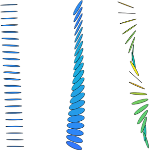
Figure 6 illustrates examples of different falling styles observed for the 3 mm disks. In the classifications of Field et al. (Reference Field, Klaus, Moore and Nori1997), these correspond to the stable mode (figure 6a), fluttering mode (figures 6(b) and 6(c), oscillating with smaller and larger amplitudes, respectively) and the tumbling mode (figure 6d). In order to identify the falling style, we quantify the angular excursion  ${\rm \Delta} p_y$, defined as the range of $p_y$ values spanned by a disk during its trajectory. Only trajectories long enough to allow for a full tumble sequence are considered in this statistic. Ideally, for steadily falling disks, ${\rm \Delta} p_y=0$, while for tumbling disks, ${\rm \Delta} p_y=2$ (assuming the trajectories are contained in a vertical plane, thus, with excursions between $p_y=-1$ and $p_y=1$); in reality, such limits are only approached. For fluttering, intermediate values of ${\rm \Delta} p_y$ are expected depending on the maximum inclination angle. This quantity captures tumbling in any direction using a single value per trajectory and yields similar results to those found using ${\rm \Delta} p_x$. Figure 7 presents histograms of ${\rm \Delta} p_y$ for the three considered disk sizes. A bimodal distribution is observed for the 1 and 3 mm disks, while for the 2 mm disks, high values of ${\rm \Delta} p_y$ dominate. The distributions do not suggest a clear threshold to define fluttering. This is especially elusive because, in the present range of physical parameters, the lateral excursions typically associated to this mode are too small to be reliably detected. Therefore, in the following we will simply denote the trajectories as ‘non-tumbling’ and ‘tumbling’ based on whether ${\rm \Delta} p_y$ is smaller or larger than 1.5, respectively. It is clear from figure 7 that the exact value of the threshold is inconsequential for such definition. We note that the bimodal behaviour of the 1 mm disks and the consistent tumbling of the 2 mm disks agree with the regime map proposed by Lau et al. (Reference Lau, Huang and Xu2018) (see figure 1). However, the same map also predicts the 3 mm disks would always tumble, which is at odds with the present observations.

Figure 6. Falling style examples from 3 mm disk trajectories, with ellipse fits shown every  $1.14 \times 10^{-3}$ s. Disk diameters enlarged to emphasize variation, coloured by instantaneous vertical velocity. Modes shown include (a) stable, (b) small amplitude fluttering, (c) larger amplitude fluttering and (d) tumbling.

Figure 7. Histograms of  $p_y$ range along individual trajectories, shown as a percentage of trajectories for the (a) 1 mm, (b) 2 mm and (c) 3 mm disks.
The non-tumbling disks favour approximately horizontal orientations, maximizing their projected area in the vertical direction. This is demonstrated in figure 8, where the probability distribution functions (PDFs) of  $|p_y|$, are plotted for the 1 and 3 mm disks and for both falling styles. (The 2 mm disks do not exhibit a statistically significant number of non-tumbling trajectories.) The axis of rotational symmetry of the non-tumbling disks is preferentially aligned to the vertical, while instances of non-tumbling disks falling edge-on are negligibly scarce.

Figure 8. Distributions of the modulus of disk orientation vector vertical component  $p_y$, separated by falling style family. Solid lines indicate non-tumbling and dashed lines indicate tumbling, for the (a) 1 mm,(b) 2 mm and (c) 3 mm disks. Here, $p_y=1$ represents a perfectly flat orientation, while $p_y=0$ represents edge-on orientation.
The tumbling disks are observed to drift laterally, in agreement with previous studies of thin falling bodies (Ern et al. Reference Ern, Risso, Fabre and Magnaudet2012). Figure 9(a) illustrates a sample trajectory for a 1 mm tumbling disk, with the distributions of  $\phi$ for the different cases shown in figure 9(b). While non-tumbling disks tend to fall with quasi-vertical trajectories, tumbling ones reach up to ${\sim }12^\circ$ and 20 $^\circ$ for the smaller and larger diameters, respectively. The broadness of the distributions largely depends on the imaged trajectories being 2-D projections of the 3-D trajectories, as illustrated in figure 10(a). Indeed, the angle $\psi$ between the 3-D trajectories and the vertical is related to the projection angle $\phi$ by
 \begin{equation} \psi = \mathrm{atan} \left(\frac{\tan \phi}{\cos \gamma} \right),\end{equation}
where  $\gamma$ is the angle between the plane containing the 3-D trajectory and the $x$–
$x$– $y$ imaging plane. Under the standard assumption that the lateral drift is caused mainly by a rotation-induced lift in the direction of $\omega _t \times u$ (where $u$ is the translational velocity; e.g. Belmonte et al. Reference Belmonte, Eisenberg and Moses1998; Fabre et al. Reference Fabre, Assemat and Magnaudet2011), we have
 $$\begin{gather} \cos\gamma = \frac{\overline{\omega_z}}{\overline{|\omega_t|}}, \end{gather}$$
 $$\begin{gather}\psi = \mathrm{atan} \begin{pmatrix}\frac{\tan \phi}{\dfrac{\overline{\omega_z}}{\overline{|\omega_t|}}}\end{pmatrix}. \end{gather}$$
Figure 9. (a) Counterclockwise-rotating 1 mm disk major axis shown in black every  $4.65 \times 10^{-4}$ s. Major axis length enlarged to emphasize rotation direction of the disk. Inclination angle $\phi$ of linear fit to red centroid trajectory defined from dashed vertical line. (b) Distributions of the absolute value of trajectory inclination angles separated by falling style, where solid lines are used for the non-tumbling disks and dashed are used for the tumbling disks.

Figure 10. (a) Schematic representation of trigonometric relations used to obtain the 3-D trajectory angle  $\psi$ from the 2-D projection $\phi$. (b) Distributions of the modulus of $\psi$ for tumbling disks, with dashed vertical lines highlighting the increasing trend in peak value for increasing $D$.
$D$.
The PDF of  $\psi$ for the different cases in figure 10(b) clearly shows that the larger disks experience a stronger lateral drift, which is expected under larger circulation. The inclination from the vertical, however, is typically smaller than 20 $^\circ$, implying that the lift is subdominant with respect to the drag. This is in contrast with the tumbling plates studied by Belmonte et al. (Reference Belmonte, Eisenberg and Moses1998), Mahadevan et al. (Reference Mahadevan, Ryu and Samuel1999) and Andersen et al. (Reference Andersen, Pesavento and Wang2005), which had lift-to-drag ratios close to unity and fell along directions close to 45 $^\circ$ from the vertical. The difference is likely due to the smaller inertia ratio in those studies, $I^*=O(10^{-1}\unicode{x2013}10^{-2})$; in the present case the moment of inertia of the surrounding fluid is relatively smaller and, thus, the coupling of rotational and translation motion (driven by the shedding of vortices at various angles of attack; see Andersen et al. Reference Andersen, Pesavento and Wang2005) is less strong. This view is consistent with our observation that $\psi$ increases for larger disks, which have smaller $I^*$.
3.2. Translational dynamics
We begin by plotting the terminal velocity  $V_t=-\langle u_y \rangle$ versus the disk diameter in figure 11. The error bars, calculated with the conservative assumption that the number of independent samples coincide with the number of experimental runs, are comparable to the symbol size in these and other logarithmic plots. They will be shown later, however, when reporting the Reynolds number and drag coefficient. Superposing the data points with trend lines for various types of frozen hydrometeors reported by Kajikawa (Reference Kajikawa1972) confirms a behaviour in line with plate crystals. The PDFs of the horizontal and vertical velocity components, $u_x$ and $u_y$, respectively, are plotted in figure 12 normalized by $V_t$. The statistics of the vertical velocities are reported in table 3, with mean and standard deviations consistent with the observations of frozen hydrometeors (Kajikawa Reference Kajikawa1972; Barthazy & Schefold Reference Barthazy and Schefold2006). For comparison, Gaussian distributions are also shown. These provide reasonable approximations of the $u_x$ distributions, while $u_y$ display strong skewness with high probability of large instantaneous fall speeds. Similar skewness of the vertical velocity was found for both rising and falling particles, but at volume fractions where the wake-mediated interaction between particles was significant (Riboux, Risso & Legendre Reference Riboux, Risso and Legendre2010; Huisman et al. Reference Huisman, Barois, Bourgoin, Chouippe, Doychev, Huck, Morales, Uhlmann and Volk2016; Alméras et al. Reference Alméras, Mathai, Lohse and Sun2017; Fornari, Ardekani & Brandt Reference Fornari, Ardekani and Brandt2018; Risso Reference Risso2018). As in those cases, here the skewness can be associated to the entrainment of the flow in the object's wake (Riboux et al. Reference Riboux, Risso and Legendre2010): larger downward fluctuations are more probable due to the rapid entrainment of ambient fluid in the wake of the falling disks that reduce the pressure difference between leading and trailing edges along with the instantaneous drag. Moreover, the coupling between translational and rotational motion (peculiar to the present case with large particle anisotropy) also plays a role: when the rotating disk is oriented edge-on, the small frontal area supports limited aerodynamic drag to contrast gravity, leading to larger downward velocities sustained by the particle inertia. This point will be further discussed in the following section. Recently, Moriche, Uhlmann & Dušek (Reference Moriche, Uhlmann and Dušek2021) looked at individual oblate spheroids falling in quiescent fluid and also found skewness towards larger downward vertical velocities for particles with $\chi =1.5$. A direct comparison to their results, however, is hampered by the different aspect ratios and density ratios.

Figure 11. Measured  $V_t$ values for disks in the current study compared with settling velocities of several plate crystal hydrometeor varieties. Red, black and blue stars represent the 1, 2 and 3 mm disks, respectively. Figure adapted from Sassen (Reference Sassen1980), with data for thick plates, plates and broad branches from Kajikawa (Reference Kajikawa1972) and for branched plates and dendrites from Kajikawa (Reference Kajikawa1975). Data from other publications digitized using WebPlotDigitizer (Rohatgi Reference Rohatgi2021).

Figure 12. Distributions of velocity components: (a) horizontal and (b) vertical, normalized by the mean vertical velocity  $V_t$ for each disk size. Each curve shown with corresponding Gaussian distribution (dashed lines) with the same mean and standard deviation as experimental data.
Table 3. Disk terminal (vertical) velocities measured in quiescent air, shown with  $\pm \sigma$. Other quantities shown include the Reynolds number, drag coefficient and Best number, all calculated from the mean $V_t$ for each disk size.

Common non-dimensional parameters used to describe the mean fall speed are listed in table 3, including the drag coefficient  $C_D = 2mg/(\rho _f A V_t^2)$ and the Best number $X=C_D Re^2$. Here, a classic formulation for $C_D$ is used that assumes equilibrium between gravity and steady drag on a flat falling disk offering the maximum projected frontal area $A={\rm \pi} D^2/4$. To explore the effect of orientation, we also define an instantaneous drag coefficient based on the instantaneous projected frontal area $A_{inst}$ and the simultaneous vertical velocity $u_y$, $C_{D,inst}=2mg/(\rho _f A_{inst} u_y^2)$. The PDFs of $C_{D,inst}$ in figure 13 exhibit long tails, reflecting the skewness of $u_y$ and the variability of $A_{inst}$. The dominant modes of the distributions are very close to $C_D$, indicating that the latter does provide a reasonable mean value representing the ensemble behaviour of all particle types.

Figure 13. Distributions of the instantaneous drag coefficient calculated as  $C_{D,inst}=2mg/\rho _f A_{inst} u_y^2$ from the instantaneous projected area of the disks in the vertical direction and the instantaneous vertical velocity. Vertical dashed lines show the (nominal) drag coefficients calculated as $C_D=2mg/\rho _f A V_t^2$ using the maximum disk projected area and the mean terminal velocity.
Figure 14 compares the observed mean fall speeds with previous laboratory results. In figure 14(a) we plot  $Re$ versus $Ga$, along with the relation $Re=Ga$ (implying $V_t=U_g$) and the empirical relation obtained by Brown & Lawler (Reference Brown and Lawler2003) (and reformulated in terms of $Re$ and $Ga$ by Cabrera Reference Cabrera2021) for spheres. As $U_g$ is the terminal velocity of a flat falling disk with unitary drag coefficient, $Re$ becoming increasingly larger than $Ga$ reflects the drop of $C_D$ with increasing disk diameter. Despite the present particles being far from spherical, the agreement with Brown & Lawler (Reference Brown and Lawler2003) is fair for the 1 and 2 mm disks. Figures 14(b) and 14(c) plot $Re$ versus $X$ and $C_D$ versus $Re$, respectively, comparing with several previous studies on disks falling in liquid fluids. The agreement deteriorates with increasing diameter (and, thus, with $Re$). Figure 14(d), on the other hand, shows that our results are consistent with the findings of Bagheri & Bonadonna (Reference Bagheri and Bonadonna2016). These authors proposed a rescaling of the data by the shape-dependent parameters $k_S$ and $k_N$ in the Stokesian and Newtonian drag regimes, respectively; see Bagheri & Bonadonna (Reference Bagheri and Bonadonna2016) for definitions. Importantly, the higher- $Re$ data in their study were obtained in air, thus, at density ratios similarly high as in the present study.

Figure 14. Red, black and blue stars represent the 1, 2 and 3 mm disks, respectively, in each of the following: (a) Reynolds number versus Galileo number with the solid black line of  $Re=Ga$ implying $C_D=1$. Empirical relation from Brown & Lawler (Reference Brown and Lawler2003) (and reformulated by Cabrera Reference Cabrera2021) shown in the black dashed line.(b) Westbrook & Sephton (Reference Westbrook and Sephton2017) plot of Reynolds number versus Best number, including data from Roscoe (Reference Roscoe1949), Willmarth et al. (Reference Willmarth, Hawk and Harvey1964), Jayaweera (Reference Jayaweera1965) and Kajikawa (Reference Kajikawa1971). (c) McCorquodale & Westbrook (Reference McCorquodale and Westbrook2021a) plot of drag coefficient versus Reynolds number, including data from Willmarth et al. (Reference Willmarth, Hawk and Harvey1964), Jayaweera (Reference Jayaweera1965) and Jayaweera & Cottis (Reference Jayaweera and Cottis1969). (d) Bagheri & Bonadonna (Reference Bagheri and Bonadonna2016) plot of corrected drag coefficient versus corrected Reynolds number, accounting for shape factors of particles such as elongation and flatness as well as density ratio between the particle and fluid. Data from other publications digitized using WebPlotDigitizer (Rohatgi Reference Rohatgi2021).
The falling style is directly connected to the aerodynamic drag, and thus, it is expected to influence the fall speed. In figure 15 we display the PDFs of the instantaneous vertical velocities, separating between non-tumbling and tumbling trajectories. The tumbling 1 mm disks fall measurably faster compared with the non-tumbling ones, while the opposite is true for the 3 mm particles. The reason for this different behaviour is unclear. We note, however, that such a difference in settling velocity is smaller than the width of the distributions.

Figure 15. Instantaneous vertical velocity distributions normalized by terminal velocity. Separated by falling style, with non-tumbling shown in solid lines and tumbling shown with dashed lines for the (a) 1 mm, (b) 2 mm and (c) 3 mm disks. Negative values indicate downward velocities.
Further insight into the translational dynamics is provided by the PDFs of the disk linear accelerations, displayed in figure 16. The mean of both horizontal and vertical components is close to zero, as expected for free-falling objects that have reached terminal velocity. Compared with Gaussian distributions, both components are highly intermittent, with a non-negligible probability of reaching tens of  $g$'s. Observations of individual realizations and joint statistics of acceleration and number density, not shown for brevity, confirm that these extreme events are not related to mutual interactions between disks. The vertical components are also strongly skewed, i.e. the probability of reaching very large downward accelerations is even higher. Both the skewness and the kurtosis of the distributions increase with increasing disk size: as the object inertia increases, the instantaneous imbalance between gravity and drag can lead to extreme accelerations, especially in the downward direction ( $a_y<0$).

Figure 16. Acceleration component distributions shown with respective Gaussian distributions (dashed lines) with the same mean and standard deviation as experimental curves. (a) Horizontal and (b) vertical, both normalized by gravity (negative values indicate downward accelerations).
The inspection of individual trajectories indicates that such extreme acceleration events are associated to phases of the motion in which the disks fall edge-on (see figure 5). This is confirmed by figure 17, which displays distributions of the instantaneous vertical accelerations (here normalized by their r.m.s. values). The results are sorted in ranges of  $|p_y|$, highlighting the differences between various orientations: when disks fall edge-on, the magnitude of the instantaneous accelerations are larger and more intermittent. Additionally, the distributions are more skewed, with relatively high probability of extreme downward accelerations. This confirms that instantaneous variability in the vertical acceleration is intrinsically related to the falling style, and to tumbling in particular.

Figure 17. Instantaneous vertical acceleration distributions of tumbling disks normalized by standard deviation of the entire dataset for each respective disk size. Curves separated by ranges of  $|p_y|$ going from edge-on orientation ( $|p_y|=0$), shown in solid dark blue, to flat falling orientation ( $|p_y|=1$), shown in dotted dark green. Results are shown for the (a) 1 mm, (b) 2 mm and (c) 3 mm disks. Negative values indicate downward accelerations.
3.3. Rotational dynamics
In order to quantify the disks’ angular velocity, we first consider the trajectory-averaged magnitude,  $\overline {|\omega _t|}$. Figure 18 shows joint PDFs (JPDFs) of $\overline {|\omega _t|}$ and the angular excursion ${\rm \Delta} p_y$. Similarly to the histograms of ${\rm \Delta} p_y$ in figure 7, the 1 and 3 mm disks exhibit a bimodal behaviour: the tumbling disks ( ${\rm \Delta} p_y > 1.5$) have angular velocities around 200 rad s $^{-1}$, while rotation rates are an order of magnitude smaller for non-tumbling ones. Although a formal distinction between the stable and fluttering mode is not attempted here, the JPDFs suggest that the latter is only statistically significant for the 3 mm disks.

Figure 18. The JPDF of  ${\rm \Delta} p_y$ values versus trajectory-averaged angular velocity for long trajectories of(a) 1 mm, (b) 2 mm and (c) 3 mm disks.
The example in figure 5 suggests that the tumbling occurs with an approximately constant rotation rate. This is confirmed in figure 19, in which various metrics to describe the rotational frequency are considered for the 2 mm case (representative of all tumbling disks in this study). Figure 19(a) shows PDFs of  $f_t=\omega _t/(2 {\rm \pi})$ for all instantaneous realizations, as well as the trajectory averaged $\overline {f}_t=\overline {|\omega _t|}/(2 {\rm \pi})$. The distribution of ${f_{\theta }=1/(2t_{\theta =0})}$ is also plotted, where $t_{\theta = 0}$ is the time elapsed between successive changes of sign of $\theta$ along each trajectory. The three distributions are sharply peaked around 36 Hz. This is consistent with the behaviour of the Lagrangian temporal autocorrelation of $p_x$,
 \begin{equation} R_{p_x}^L(\tau)=\frac{\langle p_x'(t+\tau) p_x'(t) \rangle}{\sigma_{p_x}^2(\tau)}, \end{equation}
and of  $p_y$,
 \begin{equation} R_{p_y}^L(\tau)=\frac{\langle p_y'(t+\tau) p_y'(t) \rangle}{\sigma_{p_y}^2(\tau)}, \end{equation}
where  $p_x'$ and $p_y'$ are the fluctuating $p$-component values calculated as $p_i'=p_i - \overline {p}_i$, $\sigma _{p_i}^2$ is the variance, $\tau$ is the temporal abscissa and $t$ is its generic origin (Mordant, Lévêque & Pinton Reference Mordant, Lévêque and Pinton2004b; Guala et al. Reference Guala, Liberzon, Tsinober and Kinzelbach2007). The mean and variance are both taken as the respective quantity of each individual trajectory. Only trajectories 150 frames and longer are used and all trajectories longer than that are trimmed to 150 frames. Both autocorrelations are plotted in figure 19(b), implying an oscillatory behaviour with a characteristic time scale $\sim$27 ms, in close agreement with the inverse of the dominant frequency in figure 19(a).

Figure 19. All curves plotted for the 2 mm disks only. (a) Tumbling frequency comparison between distributions of instantaneous angular velocity, trajectory-averaged angular velocity and frequency of  $\theta$ sign changes along a trajectory. (b) Lagrangian temporal autocorrelation of $p_x$ and $p_y$. Secondary peak occurs at 0.027 s, corresponding to 36.4 Hz.
The distributions of  $\overline {f}_t$ for the tumbling disks are compared in figure 20(a), displaying remarkably similar values of the dominant tumbling frequency irrespective of disk size. A common non-dimensionalization of the rotation rate is in the form of a Strouhal number $St=f_t D/V_t$ (Ern et al. Reference Ern, Risso, Fabre and Magnaudet2012); see figure 20(b). Numerical studies of falling disks and oblate spheroids in the tumbling regime found $St$ to increase with $Re$ (or $Ga$) (Fernandes et al. Reference Fernandes, Risso, Ern and Magnaudet2007; Chrust et al. Reference Chrust, Bouchet and Dušek2013), consistent with the present observation. However, those simulations reported significantly larger values ( $St=0.1\unicode{x2013}0.4$) compared with what is observed here ( $St=0.03\unicode{x2013}0.06$). This suggests that, in the present range of parameters, the tumbling rate is not set by the wake shedding frequency (which for blunt bodies is expected to yield $St=O(10^{-1})$).

Figure 20. (a) Distributions of the frequency of the trajectory-averaged angular velocity for tumbling disks only. (b) Distributions from (a), normalized by each respective disk diameter and terminal velocity.
An alternative, a priori scaling for the tumbling period can be derived from the dynamic equilibrium between drag and gravity. Within numerical prefactors of order unity (including the drag coefficient) and considering that  $\rho _d \gg \rho _f$, the force balance reads
 \begin{equation} \rho_f U^2 A \sim \rho_d A h g,\end{equation}
which defines the settling velocity scale  $U = \sqrt {\tilde {\rho } h g}$ (as in Belmonte et al. (Reference Belmonte, Eisenberg and Moses1998) and Mahadevan et al. (Reference Mahadevan, Ryu and Samuel1999), and analogous to $U_g$ within a factor $\sqrt {2}$). In writing (3.6), we have assumed Newtonian drag scaling (i.e. $C_D$ independent of $U$ and of order unity), which is supported by the results in § 3.2. Then, a characteristic time scale of the motion is given by $\tau _t = U/g = \sqrt {\tilde {\rho } h/g}$. In our experiments, $\tau _t=76$ ms independent of the disk diameter. This formulation is similar to the classic relation for the response time of spherical particles falling in a quiescent fluid, $\tau _t=V_t/g$. While such a scaling is derived for the linear motion, the translational and rotational dynamics are intimately related and are expected to be governed by similar time scales (Voth & Soldati Reference Voth and Soldati2017). The observation that $f_t \tau _t=O(1)$ for all considered disks lends support to the argument that $\tau _t$ is the time scale that determines the rotational frequency of tumbling disks in free fall, at least in the considered portion of the parameter space. We note that Mahadevan et al. (Reference Mahadevan, Ryu and Samuel1999) used a similar argument based on the gravity-drag balance to estimate the rotation rate of falling plates. However, their experiments (conducted at much higher $Re$ and smaller $I^*$) supported the kinematic relation $U \sim \omega _t D$, i.e. $\omega _t \sim \sqrt {\tilde {\rho } h g/D}$, which does not reflect our observations.
The common scaling for the tumbling frequency of falling bodies,  $St \sim {\rm const.}= O(10^{-1})$, is associated with a strong coupling between the particle kinematics and the vortex shedding in its wake (Ern et al. Reference Ern, Risso, Fabre and Magnaudet2012; Mathai et al. Reference Mathai, Lohse and Sun2020). This, however, is mostly based on observations at low $\tilde {\rho }$, where the fluid momentum is comparable to or higher than the particle momentum. In the present range of $Re$, the wake is expected to shed vortices at a non-dimensional frequency comparable to those studies; but the fluid linear and angular momentum is not sufficient to drive the particle rotation, as signalled by the relatively high $\tilde {\rho }$ and $I^*$. Rather, the tumbling frequency appears set by the dominant particle inertia and the resulting drag-gravity balance. Nevertheless, oscillations in the wake may still provide the initial seed to trigger tumbling; thus, future work should focus on similar $\tilde {\rho }$ and lower $Re$, and explore the stable-to-tumbling transition. This is experimentally challenging, as it requires capturing the orientation and rotation of sub-millimetre disks falling in air.
The fact that the 2 mm disks are the most prone to tumbling may indicate that  $Re$ and $I^*$ have competing effects in this regard. Indeed, in the present range of parameters, the respective influence of fluid inertia and particle inertia in triggering, sustaining or resisting tumbling is not trivial. It is likely that a threshold $Re$ must be exceeded to incept rotation; but the increase of complexity and loss of coherence in the wake at higher $Re$ may stabilize the motion. Likewise, while fluid forces cannot impose tumbling to particles with asymptotically large $I^*$, a minimum rotational inertia of the object appears necessary to maintain autorotation. These considerations shall be tested with a comprehensive scanning of the parameter space.
4. Conclusions
We have reported on an experimental study of thin, millimetre-sized disks falling in quiescent air. The considered range of non-dimensional parameters,  $\chi =25{-}60$, ${Re=O(10^2)}$ and $I^*=O(1)$, is relevant to the settling of snow plate crystals in the atmosphere and to several other natural and industrial processes; still, to our knowledge, it was not systematically investigated before in laboratory experiments. We did not attempt to scan the parameter space, but rather expanded the number of realizations for each considered case in order to achieve a statistical description of the process.
The falling style emerges as a non-trivial outcome of the input parameters. The 1 and 3 mm disks exhibit bimodal behaviour: either falling approximately stably and flat or tumbling with a fairly invariant rotation rate. Virtually all 2 mm disks tumble. The tendency to tumble is not monotonic with any of the non-dimensional parameters explored, signalling the complexity of the phase diagram. The bimodal behaviour, recently highlighted in numerical studies of both spherical and non-spherical settling particles, underscores the importance of obtaining a large number of realizations to statistically describe the process. The lateral drift during tumbling is stronger for the larger disks. This is explained by the fact that smaller disks have smaller  $\chi$ and, thus, larger $I^*$, implying a lesser impact of the aerodynamic torque. Rotational lift is much smaller than drag for all cases, as indicated by the angle of descent being typically smaller than 20 $^\circ$. The relatively weak lateral motion prevents the clear identification of the fluttering mode.
We remark that, in the atmospheric science literature,  $Re\approx 100$ is often quoted as a threshold below which plate crystals fall steadily. This is, however, usually assumed when (or deduced by) observing frozen cloud properties via remote sensing (Bréon & Dubrulle Reference Bréon and Dubrulle2004; Noel & Chepfer Reference Noel and Chepfer2004). The present study does not conform to this view, in that the 1 mm disks ( $Re=96$) have a much stronger tendency to tumble than the 3 mm disks ( $Re=360$). Clearly, both $Re$ and $I^*$ play important roles in determining the predominant falling style. The fact that all 2 mm disks tumble, while most of the 3 mm disks do not, suggest sharp transitions in the considered region of the phase diagram. This is to be investigated by a refined exploration of the parameter space that is outside the scope of this work.
We observe larger fall speeds than what is predicted by existing correlations based on experiments in liquids. Those are limited to much smaller  $I^*$ compared with the present study, and their results have been typically parameterized based on $Re$ (or $Ga$) alone. Our measurements instead stress how the density ratio is consequential not only for the rotational dynamics but also for settling, especially in the considered regime in which fluid inertia is relatively large. Indeed, the departure of our observations from those correlations increases with $Re$. For the disks exhibiting bimodal behaviour, tumbling and non-tumbling instances show different settling velocities. Surprisingly, the trend is different for the 1 and 3 mm disks, the former falling faster when tumbling and the latter falling slower. This may be due to qualitative differences in the wake behaviour at the different $Re$, yielding different coupling with the disk motion. This remains speculative without direct observation of the wake dynamics, whose details are below the achievable spatial resolution. Fully resolved simulations are warranted to elucidate this point.
Tumbling disks experience intense instantaneous accelerations during the phase of motion in which they fall edge-on. Still, the classic definition of drag coefficient, based on the steady-state force balance of flat falling disks, provide a fair statistical estimate for the instantaneous behaviour. Assuming similar time scales for the rotational and translational motion, we then deduce a scaling of the tumbling period  $\sim \sqrt {\tilde {\rho } h/g}$. This approximately agrees with the observed rotation rate and its independence with disk diameter, and shall be tested in future studies varying density ratio and disk thickness.
The regime we have considered is challenging to capture numerically, and some of the important dynamics may not be represented by previous experiments in liquids. Therefore, besides providing direct insight on the fundamental particle–fluid interaction, we believe the data represent a useful test case for validation. Further studies shall address open questions concerning the influence of different physical parameters. In particular, three directions appear especially interesting and potentially fruitful. First, the diameter range can be expanded, towards both smaller and larger sizes. Recent numerical studies have focused on sub-millimetre objects (e.g. Jucha et al. Reference Jucha, Naso, Lévêque and Pumir2018), and a direct comparison may shed light on dynamics that can hardly be resolved in experiments such as those presented here. This would also allow probing deeper below the threshold  $Re = 100$, whose strict validity has been questioned here. On the other hand, considering larger disks would allow testing the high- $Ga$ end of the parameter space in figure 1, and verify whether an asymptotic behaviour is reached or whether different dynamics arise. Second, in order to more efficiently probe the parameter space, one may vary the disk material and geometry independently. This would enable the independent variation of $I^*$ and $Ga$, while both have been varied simultaneously in the present study. Third and finally, it would be desirable to use lightweight materials that more closely replicate the bulk density of frozen hydrometeors, which for complex shapes is far below the one of ice (Pruppacher & Klett Reference Pruppacher and Klett2010). This would allow focusing on regimes most relevant for atmospheric science, especially if such materials were used in additive manufacturing, so as to replicate complex shapes found in frozen precipitation.
The effect of plate shape on the falling style has been highlighted by recent experiments at low  $\tilde {\rho }$ (Esteban et al. Reference Esteban, Shrimpton and Ganapathisubramani2018; Vincent, Liu & Kanso Reference Vincent, Liu and Kanso2020) and deserves to be explored at high $\tilde {\rho }$, especially in the context of the settling of frozen hydrometeors. The latter is expected to be crucially influenced by atmospheric turbulence, as recently documented by the numerical studies of Jucha et al. (Reference Jucha, Naso, Lévêque and Pumir2018), Gustavsson et al. (Reference Gustavsson, Sheikh, Naso, Pumir and Mehlig2021) and Sheikh et al. (Reference Sheikh, Gustavsson, Lévêque, Mehlig, Pumir and Naso2022) for sub-millimetre plate crystals. The effect of air turbulence on millimetre-sized disks similar to those investigated here will be the subject of a future study.
Acknowledgements
F.C. is thankful to U. Lohmann and J. Henneberger (Institute for Atmospheric and Climate Science, ETH Zürich) for several insightful discussions on frozen precipitation.
Funding
This work was supported by the US National Science Foundation (Physical and Dynamic Meteorology program) through grant NSF-AGS-1822192.
Declaration of interests
The authors report no conflict of interest.
Appendix
The quantities presented in § 3, obtained at volume fractions  $\varPhi _V = O(10^{-5})$, are not significantly different when measured at $\varPhi _V=O(10^{-6})$. For brevity, this is shown for exemplary quantities for the 2 mm disks and, in particular, the histogram of ${\rm \Delta} p_y$ (figure 21a,b), the PDF $a_y$ (figure 21c) and the PDF of $|\omega _t|$ (figure 21d). The fact that virtually all 2 mm disks tumble, irrespective of the volume fraction, indicates this is not the effect of air disturbance due to the wakes of other falling disks. This supports the claim that the objects are dilute enough to exert negligible mutual interaction.

Figure 21. Statistical comparison between two experiments performed using the 2 mm diameter disks dispersed at different volume fractions. (a) Histogram of  $p_y$ range for $\varPhi _V=1.8 \times 10^{-5}$ (as in figure 7b), compared with (b) for $\varPhi _V=2.4 \times 10^{-6}$. In (c) and (d) the solid lines indicate the volume fraction that is presented in the results of this paper, while dashed lines indicate a more dilute volume fraction tested, showing (c) the instantaneous vertical acceleration distribution and (d) the instantaneous angular velocity distribution.


 Open access