


1. Introduction
The interaction between a vortex and an interface may be considered a building block in the turbulent flow of immiscible fluids. We study this building block and show that it is prone to a Kelvin–Helmholtz (KH) instability created by surface tension. We will distinguish our flow from KH instabilities at immiscible interfaces across which a velocity jump is externally imposed. This latter class of problems has been well studied, and we begin by discussing a few studies. The effect of surface tension on the primary KH roll-up process was studied using two-dimensional numerical simulations by Fakhari & Lee (Reference Fakhari and Lee2013). The main finding was that surface tension has a stabilising effect on the flow. Hou, Lowengrub & Shelley (Reference Hou, Lowengrub and Shelley1997) showed that KH roll ups form only if surface tension is low, and the range of unstable scales diminishes with increase in surface tension. Rangel & Sirignano (Reference Rangel and Sirignano1988) showed for a KH instability that non-zero surface tension results in an increase of the stable regime. Tauber, Unverdi & Tryggvason (Reference Tauber, Unverdi and Tryggvason2002) investigated KH instability in density matched fluids at large Reynolds numbers. They find that the nonlinear roll-up at low surface tension is similar to that at zero surface tension and high surface tension results in a nearly flat interface with no roll up. Consistently across these studies, surface tension thus acts as a stabiliser, by effecting a reduction in interface length and thus suppressing KH roll-up. For a review on the stabilising effects of surface tension on the Rayleigh–Taylor and Richtmyer–Meshkov instability we refer the reader to Zhou (Reference Zhou2017a,Reference Zhoub). In fact, in a vast variety of flow situations, surface tension suppresses large wavenumber perturbations, thereby decreasing interface area. Hwang, Moin & Hack (Reference Hwang, Moin and Hack2021) showed that surface tension and the KH instability are not the only mechanisms for destabilising a jet flow. They show that viscosity and density contrasts between the jet and outer fluids are important players that can drive interface distortions by non-modal mechanisms. This work provides incentive for studying, in three dimensions, non-modal effects on the present instability.
It has long been known that the same quality of bringing about a reduction in surface area can make surface tension a destabilising agent, but in other contexts. Famously, surface tension can destabilise liquid jets and break them up into droplets by the so-called Plateau–Rayleigh instability (Rayleigh Reference Rayleigh1878). Again, this happens because of the propensity of higher surface tension to effect a reduction in surface area in a circular flow geometry. In a planar geometry, Biancofiore et al. (Reference Biancofiore, Heifetz, Hoepffner and Gallaire2017) studied two parallel interfaces separating three immiscible density matched fluids with linear shear profiles in a Taylor-Caulfield configuration. This system, which is stable without surface tension, is shown to display an instability when there is a phase lock between counter-propagating capillary waves. Thus, wave interactions cause surface tension to act as destabiliser. By a similar mechanism, surface tension at the interface in planar jets and wakes at high enough levels of shear can produce global instabilities (Tammisola, Lundell & Söderberg Reference Tammisola, Lundell and Söderberg2012).
Surface tension has occasionally been reported as giving rise to small-scale structures. Zhang et al. (Reference Zhang, He, Doolen and Chen2001) again studied the effect of surface tension on the KH instability. At high surface tension, they showed the generation of small-scale vortices in the late stages of evolution, giving rise to a positive contribution of surface tension to flow enstrophy despite a negative contribution to kinetic energy. The recent study of Tavares et al. (Reference Tavares, Biferale, Sbragaglia and Mailybaev2020) shows evidence, in Rayleigh–Taylor turbulence, of a greater preponderance of smaller scales in immiscible flows with surface tension as compared with miscible flows. Vorticity generation due to interface curvature in immiscible fluids has been studied earlier by Brøns et al. (Reference Brøns, Thompson, Leweke and Hourigan2014) and Rossi & Fuster (Reference Rossi and Fuster2021).
We propose here a new mechanism for the destabilising action of surface tension. First, the mechanism is made explicit, theoretically and in simulations, in a model flow consisting of a Lamb–Oseen vortex placed on an initially straight interface. Thereafter, its signature is demonstrated in two-dimensional turbulence simulations. Two-dimensional turbulence primarily consists of concentrated patches of vorticity, each of which attain profiles close to that of Lamb–Oseen. This is discussed further in § 4.4 and direct evidence for the relevance of Lamb–Oseen vorticity profiles is shown in Appendix C. A Lamb–Oseen vortex is thus a quintessential building block of two-dimensional turbulence. Further, the vortex is placed with its centre at an initially straight interface between two immiscible fluids. Thus the dynamics due to a single Lamb–Oseen vortex placed at an interface between two fluids is studied in the absence of gravity. This geometry bears similarity to Dixit & Govindarajan (Reference Dixit and Govindarajan2010), but that study was at zero surface tension. We show analytically how vorticity is produced by surface tension at the interface, and how this makes the flow unstable. Our direct numerical simulations (DNS) confirm our analytical predictions, and show the differences in evolution of vorticity and the interface due to surface tension and density contrast. In two-dimensional (2-D) turbulence simulations on immiscible fluids, we show the strong effect of this mechanism on the energy spectrum.
2. Problem description
Two immiscible fluids of constant densities  $\rho _0$ and $\rho _1$ lie on either side of an initially flat interface in a 2-D system. The fluids are incompressible and the continuity and momentum equations they each satisfy are
 $$\begin{gather} \frac{{\rm D} \rho}{{\rm D} t} = 0, \quad \boldsymbol{\nabla} \boldsymbol{\cdot} \boldsymbol{u} = 0, \end{gather}$$
 $$\begin{gather}\rho \frac{{\rm D} \boldsymbol{u}}{{\rm D} t} ={-}\boldsymbol{\nabla} P + \mu \nabla^2 \boldsymbol{u} + \boldsymbol{F}_{\sigma}, \end{gather}$$
where  $P$ is the pressure, $\boldsymbol {u} = \{u_{r},u_{\theta }\}$ are the radial and azimuthal velocities, respectively,
 \begin{equation} \boldsymbol{F}_{\sigma} = \sigma \kappa \delta(\boldsymbol{x}-\boldsymbol{x}_s)\boldsymbol{n},\end{equation}
is the surface tension force density,  $\sigma$ is the surface tension, $\kappa$ is the curvature, $\boldsymbol {x}=\{r,\theta \}$, the subscript $s$ stands for a location on the interface, $\delta (\cdot )$ is the Dirac delta function, $\boldsymbol {n}$ is the unit normal to the interface at $\boldsymbol {x}_s$ and $\mu$ is the viscosity. In this study, both fluids have the same viscosity. The density, $\rho$ is defined as $\rho _0 c + \rho _1(1-c)$ where $c=\{0,1\}$ is the indicator function. The interface passes through the origin. A Lamb–Oseen vortex of circulation $\varGamma$ and core radius $r_c$ is placed with its centre at the origin at time $t=0$, as shown in figure 1(a,b). When surface tension is zero, and the two fluids have identical densities, each fluid particle moves strictly in a circular path, with an azimuthal velocity given by
 \begin{equation} {U} = \frac{\varGamma}{2 {\rm \pi}r} [1- \exp({-}q)], \end{equation}
where for ease of algebra we have defined  $q \equiv (r/r_c)^2$. The total angle, $\theta _s$, swept out up to time $t$ by the interface at $r_s$, is a linearly increasing function of time given by
 \begin{equation} \theta_s = \frac{\varGamma t}{2 {\rm \pi}r_s^2} [1- \exp\{{-}q_s\}].\end{equation}
For  $r_s \gg r_c$, (2.4) reduces to ${U} = \varGamma /(2 {\rm \pi}r_s)$ for a point vortex, and an initially flat interface will wind up into an ever-tightening spiral (Dixit & Govindarajan Reference Dixit and Govindarajan2010), given by $r_s^2 \theta _s = \varGamma t$. Thus, away from the vortex core, at every instance of time, the interface describes a different Lituus spiral, which is one among the Archimedean class of spirals, as seen at a typical time in figure 1(c).

Figure 1. (a) The initial density field with an equal volume of two fluids shown in black and white. (b) The initial vorticity field, (Lamb–Oseen vortex with core radius( $r_c$) = 0.1). (c) The fluid field at a later time, when the two fluids have the same density and surface tension is vanishingly small.
The relevant non-dimensional numbers are the Weber number ( $We$), which is a ratio of the inertial force to the surface tension force, and the Atwood number ( $At$), which is a measure of the density contrast between the two fluids,
 \begin{equation} We \equiv \frac{ \bar{\rho} U_c^2 r_c}{\sigma}, \quad At \equiv \frac{\Delta \rho}{\rho_0 + \rho_1}, \quad {Re} \equiv \frac{\bar{\rho} U_c r_c}{\mu}, \end{equation}
where  $\Delta \rho = \rho _0 - \rho _1$, $\bar {\rho } = (\rho _0 + \rho _1)/2$, $U_c=\varGamma [1- \exp (-1)]/(2 {\rm \pi}r_c)$, is the azimuthal velocity of the fluid. The inertial time scale $T_c = 2{\rm \pi} r^2/\varGamma$ is representative of the wind up of the spiral, while we may expect surface tension effects to become significant beyond the time scale $T_\sigma =\sqrt {\rho r_c^3/\sigma }$. For large $We$ and in the absence of instabilities, we may neglect the effect of surface tension on the interface shape up to a non-dimensional time of
 \begin{equation} T_s = \frac{T_{\sigma}}{T_c} \sim We^{1/2},\end{equation}
and up to this time, the base velocity given by the Lamb–Oseen vortex will dictate the interface shape. We note that this is an order of magnitude estimate, and the relative importance of inertia and surface tension will depend on the radial location as well as the local curvature.
3. Vorticity generation on the interface and the KH instability
An important aspect of this dynamics is the creation of vorticity at the interface by the surface tension and by the density contrast (baroclinic torque). This may be seen with (2.2) rewritten in the vorticity formulation as
 \begin{align} \frac{{\rm D} \varOmega}{{\rm D} t} = \underbrace{\frac{1}{\rho} \boldsymbol{\nabla} \times \boldsymbol{F}_{\sigma}-\frac{1}{\rho^2} \boldsymbol{\nabla}\rho \times \boldsymbol{F}_{\sigma}}_{{\rm D}\varOmega_\sigma/{\rm D}t} \underbrace{- \frac{1}{\rho^2}\boldsymbol{\nabla} \rho \times \boldsymbol{\nabla}P}_{{\rm D}\varOmega_b/{\rm D}t} + \boldsymbol{\nabla} \times \left[ \frac{1}{\rho} \boldsymbol{\nabla} \boldsymbol{\cdot} \{\mu (\boldsymbol{\nabla} {\boldsymbol u} + \boldsymbol{\nabla} {\boldsymbol u}^T)\} \right], \end{align}
where  $\varOmega =\boldsymbol {\nabla } \times \boldsymbol {u}$ is the vorticity, here pointing in the out-of-plane direction. $\varOmega$ has contributions from the surface tension, $\varOmega _{\sigma }$, and the baroclinic term, $\varOmega _b$. $\boldsymbol {\nabla }\rho \times \boldsymbol {F}_{\sigma }$ does not contribute to the vorticity as $F_{\sigma }$ and $\boldsymbol {\nabla }\rho$ both act in the same direction. An examination of (3.1) and (2.3) makes it clear that no vorticity will be generated by a perfectly flat interface or a perfectly circular one. The generation of vorticity due to surface tension requires an interface whose curvature varies along its length. But when the shape of the interface deviates from these geometries, vorticity may be generated by both density gradients and surface tension. We investigate surface tension as a generator of vorticity, and to simplify the algebra, our analytical derivation is carried out for the inviscid case.
Integrating the first term in (3.1) at a given radial location, we obtain a time-dependent vorticity at the interface as follows. Consider  $f(r,\theta ) = r-r_s(\theta )$ which vanishes on the interface, with a normal $\boldsymbol {n} \equiv \boldsymbol {\nabla }f/|\boldsymbol {\nabla } f|$, and curvature, $\kappa \equiv -\boldsymbol {\nabla } \boldsymbol {\cdot } \boldsymbol {n}$. We have
 \begin{align} \boldsymbol{\nabla} \times \boldsymbol{F}_{\sigma} ={-}\frac{1}{r}\partial_{\theta} F_{\sigma,r} &= \frac{\sigma}{r} \partial_{\theta}\left[\frac{r_s^3 + 2r_s (\partial_{\theta} r_s)^2 - r_s^2 \partial_{\theta \theta}r_s}{[r_s^2 + (\partial_{\theta} r_s)^2]^2} \delta(r \theta - r \theta_s) \right] \nonumber\\ &= \sigma \frac{r_s^2 + 2 (\partial_{\theta} r_s)^2 - r_s \partial_{\theta \theta}r_s}{[r_s^2 + (\partial_{\theta} r_s)^2]^2} \partial_{\theta}[\delta(r \theta - r \theta_s)] \nonumber\\ &\quad + \frac{\sigma}{r} \partial_{\theta}\left[\frac{r_s^3 + 2r_s (\partial_{\theta} r_s)^2 - r_s^2 \partial_{\theta \theta}r_s}{[r_s^2 + (\partial_{\theta} r_s)^2]^2} \right] \delta(r \theta - r \theta_s), \end{align}
which on the interface given by (2.5), upon integrating in time and after considerable simplification (refer to Appendix A for details of the derivation) leads to
 \begin{align} \frac{r_c}{U_c} \varOmega_{\sigma} &= \frac{ \exp(q)[1-\exp({-}1)]}{4 We \gamma^3} \left\{ 8 (q^2 + \gamma)^2 \left(1-\frac{1}{\chi^2}\right) \right. \nonumber\\ & \quad - 2[4 q^4 + 11 q^3 + 18 q^2 + 10 q + 5 + (2 q^3 - 13 q^2 -10 q - 10) \exp(q) + 5 \exp(2q)] \nonumber\\ &\quad \left.\left(1-\frac{1}{ \chi}\right) - \gamma^2 \log \chi\right\} \delta\left(\frac{r}{r_c}\theta - \frac{r}{r_c} \theta_s\right), \nonumber\\ & \equiv \frac{\Delta U}{U_c} \delta\left(\frac{r}{r_c}\theta - \frac{r}{r_c} \theta_s\right), \end{align}
where  $\gamma = [q + 1 - \exp (q)]$, $\chi = 1+ \{ 2t_n \gamma / [q \exp (q)]\}^2$, $t_n = t/T_c$. Due to the action of surface tension, a velocity jump and a corresponding vorticity are thus created at the interface. We denote the velocity components parallel to the interface on either side by $U_{\|}$ and $U_{\|} + \Delta U$, with the jump $\Delta U$ across the interface given by (3.3). It follows that the interface must be subject to the KH instability. The contribution of the baroclinic term to the vorticity when there is a density contrast between the two fluids is given in Appendix A.2. For the complete problem, an analytical dispersion relation is not possible to write down, but approximate estimates of the instability growth rates may be written down in the two limiting regimes.
3.1. Vorticity generation and the instability in the core region
Well within the core, we have  $r\ll r_c$, so $q \ll 1$. Taylor expanding in this limit, after some algebra and retaining the first surviving term in the expansion, (3.3) reduces to
 \begin{equation} \frac{\Delta U}{U_c} \sim{-}\frac{D}{ We } t_n^2,\end{equation}
where  $D=4.5[1-\exp (-1)]$. The vorticity produced, and thus the jump in velocity, are quadratic in time and proportional to the surface tension. In this limit, the interface can be closely approximated by a straight line rotating at a constant rate. We may then write the relevant dispersion relation (Chandrasekhar Reference Chandrasekhar1981), in the case where there is no density contrast ( $At=0$), in non-dimensional form as
 \begin{equation} \frac{\omega}{k {U}_c} ={-}\frac{\Delta U} {2 U_c} \pm \left[\frac{k r_c}{2 We} - \frac{1}{4}\left\{\frac{\Delta U}{U_c}\right\}^2 \right]^{1/2}, \end{equation}
where the real and imaginary parts of  $\omega$, respectively, give the frequency and growth rate of a perturbation of wavenumber $k$. Substituting (3.4) in (3.5) we get
 \begin{equation} \frac{\omega}{k {U}_c} = \frac{D} {2 We} t_n^2 \pm \left[\frac{k r_c}{2 We} - \frac{1}{4}\left\{\frac{D}{We}\right\}^2 t_n^4 \right]^{1/2}.\end{equation}
 Note that while we derive this expression under the inviscid approximation, since there are no singular effects of viscosity in this problem, it is applicable in viscous flow at high Reynolds numbers. Since viscosity multiplies the highest derivative in the Navier–Stokes equation, in certain high Reynolds number flows this term can provide a singular perturbation to the problem, and qualitatively change the nature of the solution. These effects, however, typically occur at walls. In the absence of walls, as in the present case, we may expect that high Reynolds number viscous results will agree well with inviscid results. The first term within the square bracket stands for the standard stabilising action of surface tension, increasing with wavenumber. The second term, on the other hand, indicates the destabilising effect of surface tension. As seen from (3.6), the destabilising term is quadratic in the surface tension  $\propto 1/We^2$, while the stabilising term is only linear in this quantity.
Moreover, it is evident from (3.6) that the destabilising action of surface tension must win over its stabilising action at some time for any Weber number. In other words, the interface within the core becomes KH unstable when
 \begin{equation} t_n > \left(\frac{2 k r_c We }{D^2}\right)^{1/4}.\end{equation}
 In figure 2 we plot the growth rate of perturbations given by the imaginary part of  $\omega$ in (3.6) as a function of the wavenumber $k r_c$. It is seen that the higher the surface tension, the faster the instability grows. But at any given time, for any finite $We$, there is a cutoff wavenumber beyond which flow is stable. Equation (3.6) shows that the cutoff wavenumber depends only on $We$ and $t_n$. We observe that at $t_n =1$, the lowest surface tension ( $We=10\ 040$) is stable for all wavenumbers. However, with time, the vorticity on the interface increases in all cases, destabilising longer wavelengths even at higher $We$, as seen in figure 2(b) at $t_n=5$.

Figure 2. Non-dimensional growth rate of perturbations (  $r_c{\rm Im}(\omega )/U_c$) on the interface vs the wavenumber $kr_c$; (a) $t_n = 1$ and (b) $t_n = 5$. Here, $r_c = 0.1$ and $At = 0$. As $We$ decreases, the growth rate increases, showing the destabilising effect of surface tension.
3.2. Vorticity generation and the instability in the region outside the core
Well outside the vortex core (refer Appendix A for details),  $q \gg 1$, using (3.3) we have
 \begin{equation} \frac{\Delta U}{U_c} \sim{-}\frac{40 [1-\exp({-}1)] t_n^2 }{q^2 We } \pm \frac{t_n At}{[1-\exp({-}1)]^2 q^{3/2}}. \end{equation}
The first term on the right-hand side of (3.8) corresponds to the contribution of surface tension to the velocity jump, which is negative. The second term on the right-hand side is the contribution due to the density contrast, it is negative when the inner fluid is heavier than the outer fluid and positive otherwise. The surface tension contribution to the vorticity on the interface decrease as  $r^{-4}$ and the buoyancy contribution to the vorticity decreases as $r^{-3}$. To estimate the instability, by following a procedure analogous to Dixit & Govindarajan (Reference Dixit and Govindarajan2010), we approximate the interface as a circle of radius $r$ and perturb it at an azimuthal wavenumber $m$, to get (refer to Appendix B for details)
 \begin{align} \frac{\omega r_c}{mU_c} &= (q)^{{-}1}Q+ \left( \frac{1-At}{2}\right)\left( \frac{\Delta U}{U_c}\right)q^{{-}1/2} \nonumber\\ &\quad \pm q^{{-}1/2} \left[-\left\{\frac{(1-At) }{2m } + \left( \frac{1-At^2}{4}\right)\right\} \left(\frac{\Delta U}{U_c}\right)^2\right. \nonumber\\ &\quad - \left.\frac{(1-At) Q}{m q^{1/2}} \left(\frac{\Delta U}{U_c}\right) -\frac{At Q^2}{m q} + \frac{m}{2 q^{1/2}We} \right]^{1/2}, \end{align}
where  $Q = [1-\exp (-q)]/[1-\exp (-1)]$. On examining this expression in the light of (3.8), we see that, at $At=0$, the largest destabilising term is $O(q^{-2})$ smaller than the stabilising term, so instability is not expected. When $At>0$, however, the spiralling interface can be unstable, as found by Dixit & Govindarajan (Reference Dixit and Govindarajan2010), but now surface tension stabilises the flow at high azimuthal wavenumber. Thus, the instability within a vortex core is driven by surface tension and that outside by density differences.
4. Direct numerical simulations
4.1. Simulation details
We conduct DNS using an open-source volume of fluid code Basilisk to solve (2.1a,b) and (2.2). The surface tension force given by (2.3) is modelled as a continuum surface force in the cells containing the interface. Curvature is calculated using a heights function method. The details of the formulation are given in Popinet (Reference Popinet2018). We place a Lamb–Oseen vortex at the interface in the centre of the domain, as shown in figure 1(a,b) and allow it to evolve with time. Since our computational domain, of length  $L=5{\rm \pi} r_c$, is much larger than our vortex, the far-field boundary conditions do not affect the results. We use free-slip conditions on all sides, and have checked that periodic boundary conditions give practically indistinguishable answers. Note that our simulations include centrifugal effects of density contrast when $At \ne 0$. All simulations shown here are viscous, i.e. $\mu \ne 0$. We discretise the domain with $2048^2$ collocation points, and vary the Weber number $(We): 10\ 040, 100.4, 33.3$ and $12$. The units of $\varGamma$, $r_c$, $\bar {\rho }$, $\mu$ and $\sigma$ are arbitrary in the simulations, and care is taken to define non-dimensional numbers as done in the theory for purposes of comparison. We restrict our simulations to times over which the sum of the interfacial and kinetic energies remains constant.
4.2. Vorticity generation and the resulting instabilities
Up to a time  $t_n \sim We^{1/2}$ we expect the vorticity generated on the interface in the numerical simulations to closely follow (3.3). This is shown to be the case in figure 3(a), where $t_n=1$ and $t_n = 2$ for $We=12$. To calculate the velocity jump across the interface at the point $r_s$, we numerically integrate the vorticity along the normal. We have checked that $\Delta U$ is insensitive to grid resolution. As predicted, $\Delta U \sim t_n^2$. Interestingly, the velocity jump changes sign, going from negative to positive below $r_c$. There is one more sign change at large $r$ (not shown here), and the velocity jump in the distant spiral arms is negative again, although very small. There is a small deviation of the simulated data points from (3.3). This is to be expected since surface tension and viscous effects are neglected in the derivation of (2.5). Viscous effects in the simulation will bring about a small reduction in the velocity jump as compared with theory. Secondly, from (2.7) we expect surface tension to affect the basic interface shape significantly after a time ${\sim}We^{1/2}$. Figures 3(b) and 3(c) show the perturbation vorticity at two times, calculated by subtracting the initial vorticity from the instantaneous field. In an inviscid flow, by Kelvin's circulation theorem, the vorticity created would move with the interface for eternity. Viscous flow is quite different in this aspect and this difference is an important feature of viscous multiphase flow. In our case, because the Reynolds number is high, the vorticity stays attached to the interface for quite a while. However, later, we observe, especially in the high surface tension cases such as in figure 3(c), a peeling off of vortices from the interface. This is because the new vorticity tends to roll up, as is normal for any shear layer. To stay attached, the interface would need to roll up along with the vorticity, causing a large increase in its length. This is resisted by the interface, which becomes shorter locally and the vorticity peels off. It is seen that at the larger time, instability has set in, which is consistent with the prediction of instability when $t_n > 2.08$ for $kr_c = 2 {\rm \pi}$ by (3.4). The instability becomes visible in the simulations to the naked eye at around $t_n=5$ (see movies in the supplementary material available at https://doi.org/10.1017/jfm.2022.97). For the case where surface tension ( $We = 10040$) is much lower, the time above which instability can occur, from (3.4), is $11.19$ and for $We=12$ it is $2.08$, but because the growth rate is minuscule as predicted by equation (3.5) and shown in figure 2, an instability does not become visible during the time of our simulation. Note that in simulations $\mu \ne 0$ whereas we do the stability analysis for the inviscid case. The viscosity in the numerical simulations reduces instability growth rate somewhat.

Figure 3. Vorticity generation with  $We=12, At = 0, {Re} = 10114$. (a) Velocity jump measured across the interface, as a function of interface location within the vortex core. Symbols: DNS, line: (3.3). The perturbation vorticity from the DNS is shown for time $t_n=1$ in (b) and for $t_n = 15$ in (c). The instability is well developed by $t_n=15.$ All lengths are scaled by $r_c$.
The perturbation vorticity for  $We=10\ 040$ and $12$ is plotted in figure 4. In figure 4(a), where $At = 0$, we find, in accordance with our expectations from the discussion in §§ 3 and 4.2, that a minuscule amount of vorticity is generated on the interface but no instability happens. Further, at $r \sim r_c$, this vorticity is positive. However, for $We=12$, with $At = 0$, strong negative vorticity is generated within the core, and significant positive vorticity occurs in the vicinity of
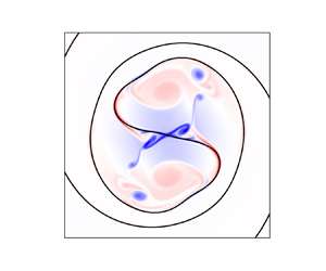
  $r \sim r_c$. As time progresses, vorticity on the interface within the core causes a KH instability, and into a breakdown into small patches of negative vorticity within the core. At even later times, as is evident from figure 4(b) positive and negative perturbation vorticities are interspersed, and dynamics in the core region appears to be chaotic. This state causes the destruction of the initial Lamb–Oseen vortex. We notice a small level of asymmetry in the vorticity contours shown in figure 4(b), and believe this to be a numerical artefact. We now examine, in figure 4(c), what happens when there is a density difference in the two fluids. It is clear that when the surface tension is low and the density contrast is high, there is a generation of alternating spirals of positive and negative vorticity in the region outside the core. The blue arms of the spiral are unstable to centrifugal Rayleigh–Taylor (CRT) modes, while the red arms are stable (Dixit & Govindarajan Reference Dixit and Govindarajan2010). At later time we see a nonlinear breakdown of the flow, as in the figure. When surface tension and density contrast are both high, just outside the vortex core, the CRT mode is stabilised by surface tension but displayed at long distances from the core, as is to be expected from our simplified theory. And the vortex gets disrupted due to the rapidly growing KH instability. We observe from figure 4(d) that the heavy fluid moves outward from the core of the vortex due to centrifugal effects. Note that the different panels of figure 4 are shown at different times. The times were chosen so as to make the instability and its nonlinear development evident.

Figure 4. Perturbation vorticity for  $We=10040$ and $12$ with and without density contrast for ${Re} = 10\ 114$: (a) $We=10\ 040$, $At = 0$ at $t_n=25$. Perturbation vorticity of small magnitude, in the neighbourhood of $r \sim r_c$, is generated. Vorticity generated within the core is small; (b) $We=12$, $At = 0$ at $t_n = 25$. The negative vorticity is mainly from the interior of the vortex; (c) $We=10\ 040$, $At = 0.05$ at $t_n = 40$. The alternating signs of density jump on the spiral arms cause alternating positive and negative vorticity; (d) $We=12$, $At = 0.5$ at $t_n = 14$. Due to the effect of either surface tension or density contrast or both, the original flow structure is disrupted in (b),(c) and (d). The black circle represents the vortex core.
4.3. Evolution of the interface
The interfaces for the cases in figure 4 are shown in figure 5. At low surface tension and zero density difference, the spiralling interface of figure 5(a) is indistinguishable from that at zero surface tension seen earlier in figure 1(c). This is because the time  $T_s$, given by (2.7), beyond which surface tension effects will be significant, is larger than our simulation time. At high surface tension, we observe from figures 4(b) and 5(b) that the interface shape is completely different from the vorticity distribution. Although vorticity is generated only at the interface, it rolls up into small-scale structures independent of the interface due to the KH instability, and with time spreads through the vortex core. The interface meanwhile adopts a relatively short and straight shape in the central region, in deference to the high surface tension. In contrast, due to the low surface tension in figure 5(c), the interface closely mimics vorticity contours of figure 4(c). Here, the CRT and KH instability are on display due to the density contrast. Far away from the core, alternating positive and negative vorticity appears on the spiral arms, indicating, from (3.8), that in this case density contrast is dominant over surface tension. Meanwhile, in the core, the vortices peel off from the interface, as a consequence of the KH instability. An important consequence of centrifugal forces is seen in figure 5(d). We started with a symmetry in the flow when rotated by the angle ${\rm \pi}$. In this image we see that this symmetry is completely broken, with the light fluid occupying the initial vortex core, and the heavy fluid having been expelled by centrifugal forces. We thus have a competition between the response to the vortex, which increases the length of the interface, and surface tension, which acts to reduce it. An independent estimate of the interface length can be obtained from energy balance. As there is no external forcing and small viscous dissipation here, the total kinetic energy is given by
 \begin{equation} \partial_t E= \langle \boldsymbol{u} \boldsymbol{\cdot} \boldsymbol{F}_{\sigma} \rangle +\epsilon_{\mu},\end{equation}
where the angled brackets refer to an average per unit area taken over the whole domain,  $E =\langle \rho u^2/2 \rangle$ and $\epsilon _{\mu }$ is the viscous dissipation rate. We also have $\langle \boldsymbol {u} \boldsymbol {\cdot } \boldsymbol {F}_{\sigma } \rangle = - ({1}/{A})\partial _t \int {\sigma dl}$, where $dl$ is an interfacial line element and $A$ is the total area of the domain (Joseph Reference Joseph1976). At high Reynolds number and significant levels of surface tension, we may neglect the viscous dissipation, to obtain
 \begin{equation} \partial_t \left(E + \frac{\sigma S}{A} \right) = 0, \quad {\rm i.e.} \ - \frac{E-E_0}{ \sigma} = \frac{S}{A}, \end{equation}
where  $S = \int \, {\rm d} l$, and $E_0$ the initial kinetic energy. We obtain the length $S$ of the interface numerically as a function of time from all four simulations, by tracking jumps in $c$ from $0$ to $1$. Obtaining the interface length correctly is a hard test for simulations. We perform this test by defining a simulation Weber number $We_c \simeq \rho U_c^2 r_c S/[A (E_0-E)]$, where the kinetic energy is obtained from the simulations. This quantity is plotted against time in figure 6(a), and is reassuringly close to the prescribed Weber number in all cases except for the highest Weber number. In this case, we do not expect an agreement, since surface tension effects are small, becoming comparable to viscous effects, which we have neglected in estimating $We_c$. We have checked in inviscid simulations (not shown) of all four cases that $We_c$ at all times is in excellent agreement with $We$. This confirms that the discrepancy at high $We$ is due to viscous effects. The test verifies the reliability of the numerics. The interface length is plotted in figure 6(b). At the highest Weber number is the practically unbridled lengthening of interface by its winding up into a spiral. As the surface tension is made higher, it competes better against the dynamics as dictated by the central vortex and suppresses the increase in interface length.

Figure 5. Regime occupied by the two fluids, one shown in black and the other in white. (a) A spiral interface is seen at  $We=10\ 040$ with $At = 0$ at $t_n=25$; (b) $We=12$, $At=0$, $t_n=25$. The fine structure is erased, and a straight interface is seen in the central portion; (c) $We=10\ 040$ with $At = 0.05$ at $t_n=40$. The CRT instability in the nonlinear regime is visible; (d) $We=12$, $At = 0.5$ at $t_n = 14$. The interface is displaced from the core of the vortex when both surface tension and density contrast are present. Here, ${Re} = 10\ 114$.

Figure 6. (a) Weber number estimated by the energy balance (symbols) compared against the actual Weber number (lines). (b) Increase in interface length (scaled by total area) with time.
4.4. Two-dimensional turbulence
To evaluate whether the mechanism we propose, of destabilisation of a flow by surface tension, is of relevance in a general 2-D turbulent flow of two immiscible fluids, we conduct DNS – at a Reynolds number ( ${Re}_T = \bar {\rho }u_{rms} L/\mu$, where $u_{rms}$ is the root mean square velocity at $t=t_i$) of $5.3 \times 10^5$ unless otherwise specified – and $At=0$ on a doubly periodic box of length $L=2{\rm \pi}$ and discretise it with $2048^2$ collocation points. We generate the initial vorticity field by first performing a single-fluid simulation. Here, we start with white noise for vorticity, and run the simulation until we attain a $k^{-3}$ scaling in the energy spectrum. Once this energy spectrum has been attained, we set the time to zero, and restart the simulation, this time with two fluids, separated by a flower-shaped interface. Such an interface shape provides some irregularity, and is obtained by superimposing a sinusoidal perturbation on a circle. The volume fraction of the minority phase is $0.225$, and simulations are conducted at four different $We_T$ ( $= \rho u^2_{rms} L/\sigma$): $\infty$, $5 \times 10^5$, $5 \times 10^4$ and $5 \times 10^3$ in runs $TR1$, $TR2$, $TR3$ and $TR4$, respectively. The initial conditions for the two-fluid simulation are shown in figure 7(a,d). The relevance to 2-D turbulence of the model flow we studied in previous sections becomes apparent when we examine figure 7(d) in some detail. We started out our single-fluid simulation with white noise, and, as expected, the vorticity organised itself primarily into concentrated patches. While some of these patches, due to the very nature of 2-D turbulence, have deviated from a circular shape, most of the vortex patches are fairly circular. Moreover, as shown in Appendix C, the vorticity profiles within the patches are well described by the Lamb–Oseen. This is not too surprising, given that Lamb–Oseen vortices are the natural steady state for a patch of vorticity (in the absence of forcing) in viscous flow, but it is reassuring to check this. Thus, studying an interface near a single Lamb–Oseen vortex is a good model for studying two-fluid turbulence. It remains to be argued why we chose a straight interface going through the centre of the vortex. This was for simplicity of algebra, and it provides the physics of the instability. It can be checked that a displaced interface, or one that is initially of a different shape, will be wound into a spiral-like shape in the vicinity of the vortex.

Figure 7. Density (a–c) and vorticity (d–f) contours for viscous simulations at  $t_i/\tau _e=9.4$ with ${Re} = 5.3 \times 10^5$. (a,d) Initial profiles, (b,e) profiles at $t^{*}/\tau _e =14.6$ for $We_T=5\times 10^5$, (c, f) profiles at $t^{*}/\tau _e =14.6$ for $We_T=5\times 10^3$ where $\tau _e = L/u_{rms} = 0.745$ is the eddy turn over time. Small-scale vortical structures occur in greater abundance as the surface tension increases. The colour scale in (d–f) has been adjusted for a better view of small-scale vorticity.
The flow consists of vortices of several scales (with vortex core radii ranging from approximately  $0.001L$ to $0.03L$), encompassing a range of Weber numbers based on each, with the largest being an order of magnitude smaller than the smallest $We_T$. Moreover, the interface is not particularly designed to pass through the centre of any vortex. So, we do not expect an exact agreement with theory, but do expect vorticity generation due to surface tension, and instabilities resulting in small-scale vortices. The regions occupied by the two fluids at $t/\tau _e=14.6$ for high and low Weber number are shown in figures 7(b) and 7(c) respectively, and the corresponding vorticity distributions are shown in figures 7(e) and 7( f) respectively. At $We_T=5 \times 10^5$, the two fluids, which displayed many spiralling interfaces at short times (see movies in the supplementary material), are mingled intricately by this time, with elongated fine structures of the inner fluid. This picture is already qualitatively different from flow at zero surface tension, in that we see vorticity generation due to surface tension along the interfaces, as predicted. But the instability, and the vorticity being peeled off from the interfaces is not yet visible. The picture is starkly different at high surface tension. There is an explosion of small-scale vorticity everywhere in the flow, and the initial vortices have been disrupted completely. Because of these small-scale vortices, there is an enhancement of energy at large wavenumbers with increase in surface tension.
The total kinetic energy in the system in shown as a function of time in figure 8(a). The two-phase simulation is started at  $t=t_i$. During the time $t< t_i$, the initial condition is prepared by running the single-phase simulation, and so this portion of the plot is not relevant to our discussion. We see that kinetic energy goes down with time. A very small part of this may be attributed to viscous dissipation whereas, especially at high surface tension, a significant part of the kinetic energy is converted to surface energy, manifested as an increase in the total length of the interface. Turbulent kinetic energy spectra (given by $E(k)=\varSigma | u_k^2|$, where $u_k$ is the velocity in spectral space) are shown in figure 8(b). With increase in surface tension, there is a significant enhancement of kinetic energy at large wavenumbers. The small-scale vorticity generated by the action of surface tension is the reason for this increase. Incidentally, earlier studies (Li & Jaberi Reference Li and Jaberi2009; Trontin et al. Reference Trontin, Vincent, Estivalezes and Caltagirone2010) have obtained a similar increase in kinetic energy with decrease in Weber number, but have not explored the underlying mechanism. The details of the instability might be different in the case of Trontin et al. (Reference Trontin, Vincent, Estivalezes and Caltagirone2010) due to vortex stretching in their case.

Figure 8. (a) The variation in time of the total kinetic energy ( $\rho u^2/2$). At $t_i/\tau _e$, we start our multiphase simulations with the flower-shaped interface and non-zero surface tension (figure 7a,d). (b) Energy spectra ( $E(k)$) versus wavenumber ( $k$) at $t^*/\tau _e$, which is shown in (a). Note that $E(k)$ is normalised in each case by $E(1)$. The fraction of energy in small scales is higher at higher surface tension. The vertical dashed lines correspond to the characteristic length scale $L_{\sigma }$ in each case. This is compared in the inset at different $We$ with the estimated length scale ( $L_{est}$). The black dash-dotted line indicates a slope of $-3$.
$-3$.
In figure 8(b), which is shown at  $t/t_e=14.6$, we had seen a significant component of energy in the small scales, and the small-scale vortices were visible in figure 7( f). We perform a consistency check now to verify that the instability due to surface tension did indeed set in well before this time. The theory is for a single vortex, so we choose the largest positive vortex (vortex 2 in figure 10b) in Appendix C. We first fit this vortex to a Lamb–Oseen vortex of appropriate circulation and width, yielding $r_c \simeq 0.2$, as shown in figure 11(b) of Appendix C. Using this and the fact that the maximum vorticity is $\varGamma /({\rm \pi} r_c^2)$ for a Lamb–Oseen vortex, we obtain $\varGamma =38.96$ and $U_c=19.6$. Thus, for this single vortex, the effective $We=768.32$ (run $TR4$). Using (3.7), and for a typical wavenumber of $kr_c=2$, we estimate the time ( $t_n= t/T_c$) above which the instability should take place as $t_n= 4.4 + t_i/\tau _e$ (we add $t_i/\tau _e$ because the two-phase simulation starts at time $t_i$). Since the inertial time scale $T_c= 0.0065$, we expect the instability should occur after $t/\tau _e = 9.783$. Indeed, in figures 7( f) and 8(b), we observe significant small-scale vorticity at $t/\tau _e = 14.6$, clearly indicating the development of an instability. The interface near smaller vortices will go unstable at earlier times than near the largest vortex. Due to the nonlinear nature of the flow, our theory cannot predict the size distribution of vortices at later times.
Another check we perform is to calculate the characteristic length scale,  $L_{\sigma }$, of a blob of the minority fluid, as a function of time, and compare it against the Hinze scale, $L_{est}$, obtained by balancing the inertial forces with the surface tension (Hinze Reference Hinze1955; Perlekar et al. Reference Perlekar, Benzi, Clercx, Nelson and Toschi2014; Mukherjee et al. Reference Mukherjee, Safdari, Shardt, Kenjereš and Van den Akker2019; Perlekar Reference Perlekar2019). The two are defined as
 \begin{equation} L_{\sigma} = 2 {\rm \pi}\frac{\varSigma_{k} C(k)}{\varSigma_{k} kC(k)} \quad {\rm and} \quad L_{est} \sim \sigma^{1/3} \beta^{{-}2/9}, \end{equation}
where the indicator function spectrum (Perlekar, Pal & Pandit Reference Perlekar, Pal and Pandit2017) is  $C(k)\equiv \sum |c_k|^2$ ( $c_k$ is the Fourier transform of indicator function $c$) and $\beta = \nu \langle |\nabla \varOmega |^2 \rangle$ is the enstrophy dissipation rate. The inset in figure 8(b) shows very good agreement between the estimated and the calculated length scales. We notice in figure 8(b) that the range of small-scale turbulence affected by the surface tension increases with surface tension, and is of the same order of magnitude as the characteristic length scale $L_\sigma$.
To quantify the chaotic mixing process and the effect of surface tension on it, we divide the domain into  $n_b=256$ equal area square boxes, $16$ in each dimension, and calculate the fraction of the minority fluid ( $a$) occupying each box. The volume fraction ( $A$) of the minority phase averaged over the entire computational domain is $0.225$, and this remains invariant in time. The probability density function (p.d.f.) $P(a/A)$ for $TR2$ and $TR4$, at low and high surface tension respectively, are shown in figure 9. It is instructive to compare these with the p.d.f. of $(a/A)$ for a circular patch of minority fluid embedded in a square patch of majority fluid, and occupying the same volume fraction of $0.225$ as in our simulations. When this square patch including both fluids is split into $n_b$ boxes, many boxes do not have minority fluid ( $a=0$) and some boxes have $a=1$, i.e. $a/A=1/0.225$, giving peaks at $a/A=0$ and $a/A=4.44$. Any entries between $a/A=0$ and $4.44$ indicate a box occupied in part by both fluids. It is clear that significant mixing has taken place due to turbulence in both $TR2$ and $TR4$. When ideally mixed, every box would have $a=A$, giving a single peak at $1$ in the p.d.f. of $a/A$, and no entries elsewhere. But we do not expect ideal mixing in our simulation, since surface tension would compete with the mixing tendency of turbulence, to minimise interface length. Therefore, it would impart to the minority fluid a tendency to form blobs. Consistent with this expectation, we see in figure 9 weaker mixing at higher surface tension. This is also consistent with the size distribution shown in Trontin et al. (Reference Trontin, Vincent, Estivalezes and Caltagirone2010), where the number of large droplets increase with the decrease in $We$.
$We$.

Figure 9. Value of  $P(a/A)$ versus $a/A$ for two runs $TR2, We = 5 \times 10^5$ and $TR4, We= 5 \times 10^3$ time averaged from $14.1\tau _e$ to $14.6\tau _e$. Black dashed line corresponds to $a/A=1$. The black solid line with circles represents the p.d.f. for a circular patch of minority fluid of the same volume fraction (=0.225) as that of the minority fluid in the simulations. As the $We$ increases, most boxes have the same volume fraction as that of the total domain.
5. Conclusion
A new role for surface tension, as a destabiliser, in the vortical flow of immiscible fluids is shown here. Due to surface tension, vorticity is generated practically everywhere on the interface, and this vorticity increases with time. It follows that the two fluid layers on either side move with different velocities, making it conducive for the KH instability to manifest itself beyond a critical time proportional to  $We^{1/4}$. This mechanism acts alongside the CRT instability when there are density differences. Our simulations on a single vortex confirm our theoretical predictions and also reveal a peeling off of small-scale vorticity from the interface. This mechanism is shown to have a significant presence in viscous simulations of 2-D turbulence at low Weber number, with an increased proportion of energy in small scales.
Supplementary material
Supplementary material is available at https://doi.org/10.1017/jfm.2022.97.
Acknowledgements
R.G. acknowledges support of the Department of Atomic Energy, Government of India, under project no. RTI4001. P.P. and R.R. acknowledge support of intramural funds at TIFR Hyderabad from the Department of Atomic Energy, Government of India, under project no. RTI4007, DST (India) Project Nos: ECR/2018/001135 and DST/NSM/R&D HPC Applications/2021/29.
Declaration of interests
The authors report no conflict of interest.
Appendix A. Derivation of the expression for vorticity on the interface
A.1. Vorticity generation due to surface tension
We define  $f(r,\theta ) \equiv r-r_s(\theta )$ which vanishes on the interface. The unit vector normal to the interface $\boldsymbol {n} = \boldsymbol {\nabla }f/|\boldsymbol {\nabla } f|$ is given by
 \begin{equation} \boldsymbol{n} = \frac{- r_s \hat{r} + \partial_{\theta} r_s \hat{\theta}}{\sqrt{r_s^2 + (\partial_{\theta} r_s)^2}}, \end{equation}
and the curvature,  $\kappa = -\boldsymbol {\nabla } \boldsymbol {\cdot } \boldsymbol {n}$, by
 \begin{equation} \kappa = \frac{r_s^2 + 2 ( \partial_{\theta} r_s)^2 -r_s \partial_{\theta \theta} r_s }{[r_s^2 + (\partial_{\theta} r_s)^2]^{3/2}}. \end{equation}
On the interface (when  $r=r_s(\theta )$), $\boldsymbol {\nabla }\times F_{\sigma }$ is
 \begin{align} \boldsymbol{\nabla} \times \boldsymbol{F}_{\sigma} ={-}\frac{1}{r}\partial_{\theta}( F_{\sigma,r}) &= \frac{\sigma}{r} \partial_{\theta}\left[\frac{r_s^3 + 2r_s (\partial_{\theta} r_s)^2 - r_s^2 \partial_{\theta \theta}r_s}{[r_s^2 + (\partial_{\theta} r_s)^2]^2} \delta(r \theta - r \theta_s) \right] \nonumber\\ &= \sigma \frac{r_s^2 + 2 (\partial_{\theta} r_s)^2 - r_s \partial_{\theta \theta}r_s}{[r_s^2 + (\partial_{\theta} r_s)^2]^2} \partial_{\theta}[\delta(r \theta - r \theta_s)] \nonumber\\ &\quad + \frac{\sigma}{r} \partial_{\theta}\left[\frac{r_s^3 + 2r_s (\partial_{\theta} r_s)^2 - r_s^2 \partial_{\theta \theta}r_s}{[r_s^2 + (\partial_{\theta} r_s)^2]^2} \right] \delta(r \theta - r \theta_s). \end{align}
Using the equation of interface given by (2.5) in (A3), we get
 \begin{align} \boldsymbol{\nabla} \times \boldsymbol{F}_{\sigma} &={-}\frac{r^6}{32a^5 \left[r^2 + \dfrac{\exp(2q)r^6 r_c^4}{4a^2 [ r^2 - \{{-}1 + \exp(q) \}r_c^2 ]^2} \right]} \left[ \frac{16a^4}{-1+\exp({-}q)( 1 + q)}\right. \nonumber\\ &\quad - \frac{8a^2\exp(3q)r^4r_c^2\{{-}4r^8-[11+ 2\exp(q)]r^6 r_c^2 + [{-}19+13\exp(q)]r^4r_c^4 \}}{(r^2 - \{{-}1 + \exp(q)\}r_c^2)^5} \nonumber\\ &\quad - \frac{8a^2\exp(3q)r^4r_c^2\{12[{-}1 + \exp(q)]r^2 r_c^6 -6[{-}1+\exp(q)^2 r_c^8\}}{(r^2 - \{{-}1 + \exp(q)\}r_c^2)^5} \nonumber\\ &\quad - \frac{\exp(5q)r^8r_c^6\{8r^8 + 10r^6r_c^2 +11r^4r_c^4 + 10r^2r_c^6 + 5r_c^8 + 5\exp(2q) r_c^8\} }{(r^2- \{{-}1 + \exp(q)\}r_c^2 )^7} \nonumber\\ &\quad - \left. \frac{\exp(5q)r^8r_c^6\{{-}2\exp(q)r_c^2 [2r^6 + 3r^4r_c^2 + 5r^2 r_c^4 + 5r_c^6 ] \} }{(r^2- \{{-}1 + \exp(q)\}r_c^2 )^7} \right]\delta(r \theta - r \theta_s). \end{align}
Note that (A3) contains terms in the  $\theta$-derivative of the delta function. Since this derivative is an odd function, its effect at the interface gets cancelled out, and it does not contribute to the vorticity.
The vorticity generated due to surface tension is obtained by integrating  $1/\bar {\rho } \boldsymbol {\nabla } \times \boldsymbol {F}_{\sigma }$ in time, to give
 \begin{align} \varOmega_{\sigma} &={-} \frac{\sigma \exp(q) {\rm \pi}^5 r_c^2}{2 \bar{\rho}\varGamma ({-}r^2 + \{{-}1+ \exp(q) \} r_c^2)^3} \left[ \frac{8\exp(4q) r^8 r_c^4 (r^4 + r^2 r_c^2 - \{{-}1+\exp(q) \} r_c^4 )^2}{( \exp(2q){\rm \pi}^2 r^4 r_c^4 )^2} \right. \nonumber\\ &\quad -\frac{8\exp(4q)r^8 r_c^4 (r^4 + r^2 r_c^2 - \{{-}1+\exp(q) \} r_c^4 )^2}{( \exp(2q) {\rm \pi}^2 r^4 r_c^4 + \varGamma^2 t^2\{ r^2 - [{-}1 +\exp(q) ] r_c^2 \}^2 )^2} \nonumber\\ &\quad + \frac{2\exp(2q)r^4 [ 4r^8 + \{ 11+2 \exp(q) \} r^6 r_c^2 - \{{-}18 + 13 \exp(q) \}r^4 r_c^4 ]}{{\rm \pi}^2 [ \exp(2q) {\rm \pi}^2 r^4 r_c^4 + \varGamma^2 t^2 \{ r^2 - [{-}1 + \exp(q) ] r_c^2\}^2 ]} \nonumber\\ &\quad - \frac{2 \exp(2q)r^4 [ 4r^8 + \{ 11+2 \exp(q) \} r^6 r_c^2 - \{{-}18 + 13 \exp(q)\}r^4 r_c^4 ]}{{\rm \pi}^2 [ \exp(2q) {\rm \pi}^2 r^4 r_c^4 ]} \nonumber\\ &\quad + \frac{2 \exp(2q)r^4 [{-}10\{{-}1 + \exp(q) \}r^2 r_c^6 + 5 \{{-}1+ \exp(q) \}^2 r_c^8 ] }{{\rm \pi}^2 [ \exp(2q) {\rm \pi}^2 r^4 r_c^4 + \varGamma^2 t^2 \{ r^2 - [{-}1 + \exp(q) ]r_c^2 \}^2 ]} \nonumber\\ &\quad - \frac{[ r^2 -\{{-}1+ \exp(q) \} r_c^2]^2 }{{\rm \pi}^4}\log \left( 1 + \left\{\frac{\varGamma^2 t^2 [ r^2 - \{{-}1 + \exp(q) \} r_c^2 ]^2}{\exp(2q) {\rm \pi}^2 r^4 r_c^4 } \right\} \right) \nonumber\\ &\quad - \left. \frac{2 \exp(2q) r^4 [{-}10\{{-}1 + \exp(q)\}r^2 r_c^6 + 5 \{{-}1+ \exp(q) \}^2 r_c^8 ] }{{\rm \pi}^2 [ \exp(2q) {\rm \pi}^2 r^4 r_c^4 ]} \right] \delta(r \theta - r \theta_s). \end{align}
Note that the vorticity due to surface tension in (A5) is the perturbation vorticity due to the surface tension as we have removed the vorticity at  $t=0$.
After some algebra, we get the perturbation vorticity due to surface tension as,
 \begin{align} \frac{r_c}{U_c} \varOmega_{\sigma} &= \frac{ [1-\exp({-}1)]\exp(q)}{4 We \gamma^3} \left\{ 8 (q^2 + \gamma)^2 \left(1-\frac{1}{\chi^2}\right) \right. \nonumber\\ &\quad - 2 [4 q^4 + 11 q^3 + 18 q^2 + 10 q + 5 + (2 q^3 - 13 q^2 -10 q - 10) \exp(q) + 5 \exp(2q)] \nonumber\\ &\quad \left.\left(1-\frac{1}{ \chi}\right) - \gamma^2 \log \chi\right\} \delta\left(\frac{r}{r_c}\theta - \frac{r}{r_c} \theta_s\right), \nonumber\\ & \equiv \frac{\Delta U}{U_c} \delta\left(\frac{r}{r_c}\theta - \frac{r}{r_c} \theta_s\right). \end{align}
 Well within the core when  $r_s \ll r_c$ or $q \ll 1$. We may set $\gamma \approx -q^2/2$, $\chi \approx 1 + [t_n q/\exp (q) ]^2$ and $\exp (q) \approx 1 + q + q^2/2 + q^3/6 + q^4/24$ in (A6) to get
 \begin{equation} \frac{\Delta U}{U_c} ={-}\frac{9 [1-\exp({-}1)] t_n^2 }{ 2 We}.\end{equation}
Outside the core,  $r_s \gg r_c$ or $q \gg 1$, $\gamma \approx - \exp (q)$ and $\chi \approx 1 + [2 t_n /q ]^2$ and we may neglect $\exp (-q)$ in (A6), so
 \begin{equation} \frac{\Delta U}{U_c} ={-}\frac{40 t_n^2 [1-\exp({-}1)]}{q^2 We }. \end{equation}
A.2. Vorticity generated by baroclinic effects
Following the approach of Dixit & Govindarajan (Reference Dixit and Govindarajan2010), we get
 \begin{equation} \frac{{\rm D} \varOmega}{{\rm D} t} = \frac{1}{\rho} \boldsymbol{\nabla} \times \boldsymbol{F}_{\sigma} - \frac{ \boldsymbol{\nabla} \bar{\rho}}{\bar{\rho}} \times\left(\frac{ \bar{U}^2}{r} \hat{r} \right) + \frac{1}{\rho} \nabla^2 \varOmega. \end{equation}
Density contrast can only contribute to vorticity at the interface when the interface departs from a circular shape, just as baroclinic torque is only created on an interface inclined to the horizontal. We obtain this departure in terms of the angle  $\alpha$ made by the interface, with a circle whose origin is at the centre of the vortex
 $$\begin{gather} \tan \alpha = \frac{{\rm \pi} r^2}{\varGamma t \{{-}1 + \exp({-}q)(1+q)\}}, \end{gather}$$
 $$\begin{gather}\sin \alpha = \frac{{\rm \pi} r^2}{[ \varGamma^2 t^2 \{{-}1 + \exp({-}q)(1+q)\}^2 + {\rm \pi}^2 r^4 ]^{1/2}}. \end{gather}$$
Using  $\boldsymbol {\nabla } \bar {\rho } = \pm \Delta \rho \delta (r\theta - r \theta _s) \boldsymbol {n}$, where $\boldsymbol {n}$ is the normal to the interface, to calculate the contribution of baroclinic term to the vorticity, we get
 \begin{equation} \frac{ \boldsymbol{\nabla} \bar{\rho}}{\bar{\rho}} \times\left(\frac{ \bar{U}^2}{r} \hat{r} \right) ={\pm} \frac{\Delta \bar{\rho}}{\bar{\rho}} \frac{\bar{U}^2}{r} \sin \alpha \delta(r \theta - r \theta_s). \end{equation}
Assuming  $\zeta = -1 + \exp (-q)(1+q)$ we rewrite (A12) as
 \begin{align} \frac{{\rm D} ( \varOmega_b)}{{\rm D} t} \approx \frac{\boldsymbol{\nabla} \bar{\rho}}{\bar{\rho}} \times \left(\frac{\bar{U}^2}{r} \hat{r} \right) = \frac{At \varGamma^2 [1-\exp({-}q)]^2}{4{\rm \pi} r} \frac{1}{( \varGamma^2 t^2 \zeta^2 + {\rm \pi}^2 r^4 )^{1/2}} \delta(r\theta -r \theta_s). \end{align}
We obtain  $\varOmega _b$ by integrating (A13),
 \begin{equation} \varOmega_b(r,t) = \frac{At \varGamma [1-\exp({-}q)]^2}{4{\rm \pi} r \zeta} \tanh^{{-}1} \left[ \frac{\varGamma \zeta t}{\left( \varGamma^2 t^2 \zeta^2 + {\rm \pi}^2 r^4 \right)^{1/2}} \right] \delta(r\theta -r \theta_s). \end{equation}
In non-dimensional form, the above equation can be rewritten as
 \begin{align} \frac{\varOmega_b(r,t) r_c}{U_c} = \frac{At [1-\exp({-}q)]^2}{2[1-\exp({-}1)]^2 q^{1/2} \zeta} \tanh^{{-}1} \left[ \frac{2t_n \zeta}{\{ 4 t_n^2 \zeta^2 + q^2 \}^{1/2}} \right] \delta\left(\frac{r}{r_c} \theta - \frac{r}{r_c} \theta_s \right). \end{align}
Far away from the vortex core or  $q \gg 1$, $\zeta \approx -1$ , $\exp (-q) \approx 0$ and $\tanh ^{-1}[x/\sqrt {1+x^2}] \approx x - x^3/6$, where $x = 2t_n \zeta /q$ so
 \begin{equation} \frac{\Delta U}{U_c} \approx{\pm} \frac{At [1-\exp({-}q)]^2}{2[1-\exp({-}1)]^2 q^{1/2} \zeta}\left[ \frac{2t_n}{q} - \frac{8t_n^3}{q^3} \right]. \end{equation}
When  $q \gg 1$, we drop the terms with $q^{-3}$ so,
 \begin{equation} \frac{\Delta U}{U_c} \approx{\pm} \frac{t_n At}{[1-\exp({-}1)]^2 q^{3/2} }. \end{equation}
Appendix B. Dispersion relation away from the core of the vortex
Upon linearising (2.2) about the base flow, using normal mode analysis and following the approach given by Dixit & Govindarajan (Reference Dixit and Govindarajan2010), we obtain
 \begin{align} &\bar{\rho} \left[ \left(\omega - \frac{m\bar{U}}{r} \right)\left\{ \frac{1}{r} \partial_r \left[\frac{r^2}{m}\left(\partial_r u_r + \frac{u_r}{r}\right)\right] - \frac{m}{r} u_r\right\} + u_r \partial_r \bar{\varOmega} \right] \nonumber\\ &\quad ={-}\partial_r\bar{\rho} \left[ \frac{r}{m}\left( \omega - \frac{m\bar{U}}{r}\right)\left( \partial_r u_r + \frac{u_r}{r}\right) + u_r \left( \partial_r \bar{U} + \frac{\bar{U}}{r}\right) \right] \nonumber\\ & \qquad - \frac{m\bar{U}^2 \partial_r \bar{\rho} }{r^2\left(\omega - \dfrac{m\bar{U}}{r}\right)}u_r +\frac{\sigma u_{rs}}{\left(\omega - \dfrac{m\bar{U}}{r}\right)}\left(\frac{m}{r}\right)^3 \delta(r-r_s), \end{align}
where  $u_r$ is the perturbation velocity in the azimuthal direction and $u_{rs}$ is the velocity at $r_s$.
Using all the boundary and jump conditions similar to Dixit & Govindarajan (Reference Dixit and Govindarajan2010), we get the dispersion relation at  $r$ as
 \begin{align} \omega &= \frac{m}{r(\rho_0 + \rho_1)} [ \rho_0 \bar{U}_0 + \rho_1 (\bar{U}_0 + \Delta U)] \pm \left[-\frac{m}{r^2(\rho_1 + \rho_0)}\{ \rho_0 \bar{U}_0^2- \rho_1 (\bar{U}_0 + \Delta U)^2\} \right. \nonumber\\ & \quad \left.+ \frac{m^3\sigma}{r^3(\rho_0 + \rho_1)} - \frac{m^2 \rho_0 \rho_1 (\Delta U)^2}{r^2(\rho_0 + \rho_1)^2}\right]^{1/2}, \end{align}
where  $\bar {U}_1 = \bar {U}_0 + \Delta U$ and $\bar {U}_0$ and $\bar {U}_1$ are the velocities of $\rho _0$ and $\rho _1$ fluids at the jump near a given $r$. In the absence of surface tension ( $\sigma = 0$), this reduces to the one given in Dixit & Govindarajan (Reference Dixit and Govindarajan2010).
In non-dimensional form the dispersion relation will be of the form
 \begin{align} \frac{\omega r_c}{mU_c} &= (q)^{{-}1}Q+ \left( \frac{1-At}{2}\right)\left( \frac{\Delta U}{U_c}\right)q^{{-}1/2} \nonumber\\ &\quad \pm q^{{-}1/2} \left[-\left\{\frac{(1-At) }{2m } + \left( \frac{1-At^2}{4}\right)\right\} \left(\frac{\Delta U}{U_c}\right)^2\right. \nonumber\\ &\quad \left.- \frac{(1-At) Q}{m q^{1/2}} \left(\frac{\Delta U}{U_c}\right) -\frac{At Q^2}{m q} + \frac{m}{2 q^{1/2}We} \right]^{1/2}, \end{align}
where  $Q = [1-\exp (-q)]/[1-\exp (-1)]$.
Appendix C. Two-dimensional turbulence – presence of Lamb–Oseen vortices
We had chosen to study a Lamb–Oseen vortex as a suitable building block of 2-D turbulence. We now show that this choice is appropriate. It is known that the Lamb–Oseen profile is an attracting solution for a patch of vorticity in isolation. Indeed in 2-D turbulence (if there were no interface), despite its highly nonlinear nature, the flow may be described well by a distribution of discrete vortex patches. Further, these patches are often practically Lamb–Oseen vortices. To make this visually evident, we started our 2-D decaying turbulence simulation on a single fluid phase, with white noise as the initial condition for vorticity as shown in figure 10(a). The system, as we know it should, spontaneously evolves into concentrated patches of vorticity, as seen in figure 10(b) at time  $t_i$. While the nature of turbulence makes these vortices depart somewhat from axisymmetry, their profiles for the most part are remarkably close to Lamb–Oseen, as demonstrated for two sample vortices in figure 11. The shape of the sample vortices is similar to the isolated vortex shape given in McWilliams (Reference McWilliams1984).

Figure 10. (a) The initial condition of vorticity for the single-phase decaying turbulence simulation. (b) Vorticity at  $t_i/\tau _e$ at which time the two-phase simulation is initiated.

Figure 11. Comparison of the vorticity profile for vortices 1,2 shown in figure 10(b) with the best fitting Lamb–Oseen vortex (Gaussian). Vorticity variation along  $x$ and $y$ for (a) vortex 1 and (b) vortex 2. The black dashed lines represent the fit to a Lamb–Oseen vortex $\varOmega \equiv \varOmega _0 \exp (-q)$, where $\varOmega _0$ is the maximum vorticity and $q = (x^2 + y^2)/r_c^2$. The origin in each case is at the vortex core.


