


1. Introduction
Fluids exceeding the critical pressure,  $p_c$, are ubiquitous in many environmental and engineering settings. Well-known natural occurrences exist in the atmosphere of Venus (Lebonnois & Schubert Reference Lebonnois and Schubert2017) as well as subsurface flows near terrestrial undersea volcanoes (Parisio et al. Reference Parisio, Vilarrasa, Wang, Kolditz and Nagel2019). Technical applications include fluids used in chemical impregnation and extraction processes, chromatography, and polymer processing (Knez et al. Reference Knez, Markočič, Leitgeb, Primožič, Hrnčič and Škerget2014). Especially in many industrial applications, high-pressure fluids are also subject to significant heat transfer, with convective heat transfer being a dominant mechanism for energy transport. Examples of such applications include power generation systems and heat engines (Wang et al. Reference Wang, Zhang, Yu, Wang, Shi and Chen2019; Yu et al. Reference Yu, Yang, Wang, Shi and Chen2019). Additionally, the operational designs of many energy conversion systems under development are predicated on efficient heat transfer with working fluids at supercritical pressures, including regenerative cooling in rocket engines (Ruan & Meng Reference Ruan and Meng2012), nuclear reactor coolant systems (Yoo Reference Yoo2013), and supercritical water oxidation (Pizzarelli Reference Pizzarelli2018).
For the large temperature ranges found in many technical and environmental applications, many such high-pressure fluids exist at transcritical conditions. At these conditions, the pressure  $p$ exceeds $p_c$ but the temperature $T$ straddles the critical temperature $T_c$. In transcritical fluids, a number of non-ideal effects have been observed when the reduced pressure $p_r \equiv p/p_c$ and the reduced temperature $T_r \equiv T/T_c$ approach unity. Transitioning from the liquid-like to gas-like regions, the density, viscosity and diffusivity display sharp gradients, while the isothermal compressibility, specific heat capacity and thermal conductivity exhibit pronounced peaks (Clifford & Williams Reference Clifford and Williams2000; Kiran, Debenedetti & Peters Reference Kiran, Debenedetti and Peters2012). These behaviours are illustrated in figure 1, which shows thermoviscous properties – density $\rho$, constant-pressure specific heat capacity $c_p$, thermal conductivity $\lambda$, and dynamic viscosity $\mu$ – of nitrogen for different supercritical pressures.

Figure 1. Thermoviscous properties of nitrogen at various supercritical pressures as a function of reduced temperature. Data taken from NIST (Linstrom & Mallard Reference Linstrom and Mallard2017). (a) Thermodynamic properties: density  $\rho$ and constant-pressure specific heat capacity $c_p$ plots. (b) Transport properties: thermal conductivity $\lambda$ and dynamic viscosity $\mu$ plots.
At turbulent conditions in the transcritical regime, the presence of both liquid-like and gas-like thermodynamic property dependencies yields two spatial regions in the fluid domain, each with distinctive behaviour as influenced by the thermodynamics. Compared with classical constant-property trends, observations of turbulence in the gas-like region have shown – among other features – increased overall streamwise and spanwise anisotropy, enlarged spanwise spacing of large-scale near-wall structures (Patel et al. Reference Patel, Peeters, Boersma and Pecnik2015), and intensified relative turbulent fluctuation levels of thermodynamic transport properties (Kim, Hickey & Scalo Reference Kim, Hickey and Scalo2019). Reverse trends have been observed in the liquid-like regime. In addition, at the transition between liquid-like and gas-like conditions, particularly abrupt variations in thermodynamic properties induce sharp increases in turbulent fluctuations to further alter the flow dynamics. Overall, the coupling between the transcritical property variations and the turbulence dynamics yields behaviours that contrast with those of the more extensively-studied compressible turbulent wall-bounded flows that are well-described as ideal gases.
Additionally, in realistic transcritical flows, these coupled effects of modulated turbulence and property variations can be combined with a number of other physical phenomena, including thermoacoustic oscillations and buoyancy, all of which contribute towards further modification of the resultant turbulence dynamics and heat transfer, as discussed in Kim et al. (Reference Kim, Hickey and Scalo2019) and Nemati et al. (Reference Nemati, Patel, Boersma and Pecnik2015). The presence of buoyancy effects can cause transcritical fluids to undergo significant reduction in the magnitude of heat transfer. Known as heat transfer deterioration, this is a phenomenon that is known to arise from reduced turbulence production and decreased near-wall fluid density (Pizzarelli Reference Pizzarelli2018), but which current analytical models and correlations have not been able to successfully predict (Yoo Reference Yoo2013). In recent decades, while the momentum behaviour of turbulence has been examined thoroughly for both variable-property and constant-property wall-bounded flows, the detailed characterization of the thermal transport is not nearly as well understood (Patel, Boersma & Pecnik Reference Patel, Boersma and Pecnik2017). Further physical study and understanding are necessary to predict accurately the temperature statistics and associated heat transfer in transcritical flows.
The complex interplay of the physical processes that are present in turbulent transcritical flows poses a number of challenges when investigating the heat transfer. Experimental measurements at such conditions lack spatial and temporal resolution; the available data are mostly limited to averaged heat transfer quantities with minimal information on turbulence statistics (Ma, Yang & Ihme Reference Ma, Yang and Ihme2018). Presently, models used in Reynolds-averaged Navier–Stokes (RANS) methods for transcritical fluids are unable to predict accurately flow statistics of interest, particularly for heat transfer values (Yoo Reference Yoo2013). Current wall-modelled large eddy simulation (WMLES) techniques have been developed largely to simulate ideal gas flows (Ma et al. Reference Ma, Yang and Ihme2018) and thus are not suited for calculations in transcritical conditions. With such constraints, current and ongoing investigations of turbulence in transcritical fluids are predominantly direct numerical simulation (DNS) studies that resolve the full range of turbulent scales in the flow.
Efforts to characterize the thermal boundary layer have led to the development of the temperature law of the wall as a thermal analogy of the well-known velocity law of the wall. The temperature law of the wall, first proposed by von Kárman (Reference von Kárman1939), is a functional relation for the mean temperature difference  $\bar {\theta } = | \bar {T} - T_w|$, where $T$ is the fluid temperature, $T_w$ denotes the temperature at the wall, and $\bar {\cdot }$ indicates averaging over homogeneous and steady-state conditions. A general analytical form of the temperature law of the wall, which can be obtained through scaling arguments, is expressed as (Kader Reference Kader1981)
 \begin{equation} \bar{\theta}^+{=} \left\{ \begin{array}{@{}ll} \overline{Pr} \, \zeta^+, & \text{viscous sublayer}, \\ \dfrac{1}{\kappa_T} \, \ln \zeta^{+} + \beta (\overline{Pr}), & \text{logarithmic (log) region}, \end{array} \right. \end{equation}
where  $\overline {Pr} = \overline { c_p \mu / \lambda }$ is the averaged Prandtl number, $\kappa _T$ is a constant, and $\beta (\overline {Pr})$ is a function of $\overline {Pr}$; $\zeta$ is a modified wall-normal coordinate that provides the distance from the pertinent wall. The superscript ‘ $+$’ on $\zeta$ and $\bar {\theta }$ indicates quantities measured in wall units, via normalization by friction quantities as
 \begin{equation} \zeta^+{\equiv} \frac{\zeta \sqrt{\tau_w \rho_w}}{\mu_w} = \frac{\zeta u_\tau}{\nu_w} \end{equation}
and
 \begin{equation} \bar{\theta}^+{\equiv} \frac{\bar{\theta} \rho_w c_{p,w} u_\tau}{q_w} = \frac{\bar{\theta}}{T_\tau} = \frac{|\bar{T} - T_w|}{T_\tau}, \end{equation}
where  $\tau _w \equiv |\mu \, \partial u/\partial y|_w$ is the wall shear stress, $u_\tau \equiv \sqrt {\tau _w / \rho _w}$ is the friction velocity, $q_w \equiv |\lambda \, \partial T / \partial y|_w$ is the wall heat flux, $\nu _w \equiv \mu _w / \rho _w$ is the kinematic viscosity evaluated at the wall, and $T_\tau \equiv q_w / (\rho _w c_{p,w} u_\tau )$ is the friction temperature. The subscript $w$ indicates variables evaluated at the wall, or calculated using averaged quantities that are then evaluated at the wall when applicable. Here, $y$ is a global wall-normal coordinate. For historical context, the approach of using self-similarity methods to obtain the temperature law of the wall closely resembles the development of the Monin–Obukhov (MO) similarity theory (Monin & Obukhov Reference Monin and Obukhov1954). In the surface layer of the atmospheric boundary layer, the MO similarity theory utilizes the near-constant vertical fluxes to describe successfully the wind speed and temperature profiles in stable boundary layers. Even with considerations for buoyancy-driven physics, the MO similarity theory also yields a log-linear profile that remains similar in form to (1.1) (Stull Reference Stull1988).
The viscous sublayer solution of (1.1) is well characterized for a broad range of flows. In contrast, there is currently no consensus regarding a consistent representation of the logarithmic region. The most successful and widely-used correlation was developed by Kader (Reference Kader1981), who employed an assumption of constant turbulent Prandtl number in the logarithmic region and arrived at the expressions  $\kappa _T = 0.4717$ and $\beta (\overline {Pr}) = (3.85 \overline {Pr}^{1/3} - 1.3 )^2 + \ln (\overline {Pr}) / \kappa _T$. In flows with spatially homogeneous $\overline {Pr}$, Kader's correlation agrees well with mean temperature profiles from experimental data for $0.7 \leq \overline {Pr} \leq 170$, for data from fully developed turbulent flows in flat-plate boundary layers (Simonich & Bradshaw Reference Simonich and Bradshaw1978; Blair Reference Blair1983) and in channels (Kader Reference Kader1981). Agreement with numerical data has also been observed in DNS (Kim & Moin Reference Kim and Moin1989; Pirozzoli, Bernardini & Orlandi Reference Pirozzoli, Bernardini and Orlandi2016; Abe & Antonia Reference Abe and Antonia2017) as well as in RANS and large eddy simulation (LES) settings (Duponcheel et al. Reference Duponcheel, Bricteux, Manconi, Winckelmans and Bartosiewicz2014; van Cauwenberge et al. Reference van Cauwenberge, Schietekat, Floré, Van Geem and Marin2015). However, characterizing the mean temperature profile using Kader's correlation in other flow set-ups has shown a number of deficiencies, specifically in characterizing the logarithmic region quantitatively. This poor agreement is seen in flows with strong temperature gradients (Toutant & Bataille Reference Toutant and Bataille2013), in chemically reacting flows (Artal & Nicoud Reference Artal and Nicoud2006), and in flows with strongly varying thermodynamic properties (Patel et al. Reference Patel, Boersma and Pecnik2017; Guo, Yang & Ihme Reference Guo, Yang and Ihme2018).
In the following, we review the relevant body of literature for variable-property wall-bounded DNS studies that attempt to characterize the mean temperature profile. We introduce here the density ratio,  $\varOmega$, defined as $\varOmega \equiv \rho _{cold}/\rho _{hot}$, with $\rho _{cold}$ being the density at the cold wall and $\rho _{hot}$ being the density at the hot wall. A number of early numerical simulations of variable-property flows have considered relatively small $\varOmega$ values of $O(1)$ and simplified thermodynamics wherein one or more transport properties are either held constant artificially or prescribed by a simplified algebraic dependence on temperature. While general insight into the behaviour of the temperature profile in variable-property turbulence was accessible from these early studies, limited understanding is available into the more extreme conditions that are representative of typical transcritical turbulence in real-world applications (with $\varOmega$ values of $O(10\text {--}100)$). Nicoud (Reference Nicoud1998) and Nicoud & Poinsot (Reference Nicoud and Poinsot1999) performed simulations of variable-property isothermal wall channels with $\varOmega = 2$ and showed significant deviation from Kader's mean temperature correlation. Later, Patel et al. (Reference Patel, Boersma and Pecnik2017) analysed a set of nine variable-density turbulent channel flows with $\varOmega \lessapprox 2.5$, and showed that both Kader's correlation and a proposed modification developed through the analysis by Lee et al. (Reference Lee, Jung, Sung and Zaki2014) for flat-plate turbulent boundary layers have limited success in representing the mean temperature accurately. Instead, Patel et al. (Reference Patel, Boersma and Pecnik2017) proposed an ‘extended van Driest transformation’ for the mean temperature profile, demonstrating good collapse across cases with different behaviours of the semi-local friction Reynolds number $Re_\tau ^* = \bar {\rho } \sqrt {\tau _w / \bar {\rho }} \, L_y / \bar {\mu }$ but constant $\overline {Pr}$. Here, $L_y$ is the channel half-height.
Recent computational investigations have utilized more realistic thermodynamic models in an effort to examine conditions that are more representative of real-world transcritical turbulence. Toki, Teramoto & Okamoto (Reference Toki, Teramoto and Okamoto2020) presented results for turbulent transcritical channel flow calculations at density ratios  $\varOmega =4$ and $\varOmega =8$ before proposing a mixing-length model to transform the mean temperature profile. Comparisons of results from their transformation with incompressible DNS data by Morinishi, Tamano & Nakamura (Reference Morinishi, Tamano and Nakamura2007) appeared successful, conditional on allowing the amount of shift in the logarithmic region to be fitted empirically a posteriori. Wan et al. (Reference Wan, Zhao, Liu, Wang and Lei2020) presented channel flow simulations of transcritical carbon dioxide with a maximum density ratio $\varOmega \approx 3$. They then extended the capabilities of Patel et al. (Reference Patel, Boersma and Pecnik2017)'s ‘extended van Driest transformation’ to include the effects of variable $c_p$. These more recent studies demonstrate relative success in the characterization of the mean temperature profile and other temperature statistics, but still at limited ranges of density ratios and heating conditions examined. At the transcritical conditions relevant to practical applications, current modelling efforts have not yet demonstrated confidence in the ability to characterize or predict temperature statistics.
To address this issue, this investigation provides a detailed analysis of DNS calculations of fully developed transcritical turbulent channel flow, with a focus on the analysis of the thermal boundary layer. Our calculations involve (1) a compressible Navier–Stokes formulation, (2) realistic thermodynamic considerations to represent accurately the behaviour of state variables and transport properties in the transcritical regime, and (3) density ratios  $\varOmega$ of up to $O(20)$ to better represent the behaviour of transcritical turbulence in real-world settings. The main objective of this study is to provide a theoretical framework to best characterize the mean temperature profile in the logarithmic region. As a secondary objective, we provide observations of the turbulent statistics and structures of the thermal flow field, and how they are affected by the operating conditions.
The remainder of this paper is organized as follows. Section 2 presents the problem formulation, which includes details of the governing equations, model relations utilized, domain definition and overall computational set-up. Section 3 presents results from the simulations along with associated interpretations, discussions, and modelling efforts. Finally, § 4 offers conclusions.
2. Problem formulation
2.1. Governing equations, thermodynamic models, and domain definition
The governing equations that are solved are the conservation equations of mass, momentum and total energy:
 \begin{gather} \frac{\partial \rho}{\partial t} + \frac{\partial \left( \rho u_j \right)}{\partial x_j} = 0, \end{gather}
 \begin{gather}\frac{\partial \left(\rho u_i \right)}{\partial t} + \frac{\partial \left( \rho u_i u_j \right)}{\partial x_j} ={-} \frac{\partial p}{\partial x_i} + \frac{\partial \tau_{ij}}{\partial x_j} + f_i, \end{gather}
 \begin{gather}\frac{\partial \left(\rho e_t \right)}{\partial t} + \frac{\partial \left( \rho u_i e_t \right)}{\partial x_i} ={-} \frac{\partial \left( u_i p \right)}{\partial x_i} + \frac{\partial \left( \tau_{ij} u_i \right)}{\partial x_j} - \frac{\partial q_i}{\partial x_i} + u_i f_i, \end{gather}
where  $u_i$ is the $i$th component of the velocity vector, $p$ is the pressure, and $e_t$ is the total specific energy, combining the specific internal energy $e$ and the specific kinetic energy $(u_i u_i)/2$. Here, $\,f_i$ is the $i$th component of the body force vector, which imposes a prescribed bulk streamwise momentum. This body force vector serves as a streamwise-homogeneous substitute for a pressure gradient. For the Reynolds numbers in the current investigation, the choice of a body force to replace a conventional pressure gradient has a negligible effect on the pressure drop from skin friction. Previous authors (Huang, Coleman & Bradshaw Reference Huang, Coleman and Bradshaw1995; He, He & Seddighi Reference He, He and Seddighi2016; Quadrio, Frohnapfel & Hasegawa Reference Quadrio, Frohnapfel and Hasegawa2016) have shown additionally that characteristic turbulence statistics are largely robust to the choice of forcing scheme. Following Huang et al. (Reference Huang, Coleman and Bradshaw1995), $f_i$ is written as
 \begin{equation} f_i ={-}\frac{\Sigma \tau_w}{2 L_y}\,\frac{\bar{\rho}}{\rho_0}\,\delta_{1i}, \end{equation}
where the direction  $i = 1$ indicates the streamwise direction, the subscript ‘ $0$’ denotes a volume-averaged quantity, and $\delta _{ij}$ is the Kronecker delta operator. Here, $\tau _{ij}$ is the viscous stress tensor defined as
 \begin{equation} \tau_{ij} = \mu \left(\frac{\partial u_i}{\partial x_j} + \frac{\partial u_j}{\partial x_i} \right) - \frac{2}{3} \mu\,\frac{\partial u_k}{\partial x_k}\,\delta_{ij}, \end{equation}
and  $q_i$ is the heat flux vector given as
 \begin{equation} q_i ={-}\lambda\,\frac{\partial T}{\partial x_i}, \end{equation}
where  $\lambda$ is the thermal conductivity.
The working fluid considered is nitrogen (N $_2$) with critical pressure $p_c = 3.3958$ MPa, critical temperature $T_c = 126.19$ K, molecular weight $W = 28.0134$ g mol $^{-1}$, and acentric factor $\omega = 0.0372$.
We close the system of equations with the Peng–Robinson (PR) equation of state (EoS) (Peng & Robinson Reference Peng and Robinson1976; Poling, Prausnitz & O'Connell Reference Poling, Prausnitz and O'Connell2001), which has been used widely in supercritical and transcritical settings because of its accuracy in predicting thermodynamic state variables in the vicinity of the critical point (Miller, Harstad & Bellan Reference Miller, Harstad and Bellan2001). At transcritical conditions comparable to those used in our investigation, Peng & Robinson (Reference Peng and Robinson1976) reports root-mean-square (r.m.s.) errors below  $1.25\,\%$ in enthalpy departure prediction when compared to experimental values, while Congiunti & Bruno (Reference Congiunti, Bruno and Giacomazzi2003) and Hickey et al. (Reference Hickey, Ma, Ihme and Thakur2013) show results with similar error levels when representing $\rho$ and $c_p$. The PR EoS is expressed as
 \begin{equation} p = \frac{\rho RT}{1-b \rho} - \frac{\rho^2 a}{1 + 2 b \rho - b^2 \rho^2}, \end{equation}
where  $R$ is the gas constant. The parameters $a$ and $b$ account for real fluid effects and are given as
 \begin{gather} a = 0.457236\,\frac{R^2 T_c^2}{p_c} \left[ 1 + c \left( 1 - \sqrt{\frac{T}{T_c}} \right) \right]^2, \end{gather}
 \begin{gather}b = 0.077796\,\frac{R T_c}{p_c}, \end{gather}
with
 \begin{equation} c = 0.37464 + 1.54226 \omega - 0.26992 \omega^2, \end{equation}
and with  $\omega$ being the previously introduced acentric factor. For N $_2$,
$_2$,  $b = 8.58 \times 10^{-4}$ and $c = 0.432$.
Chung's model for high-pressure fluids (Chung, Lee & Starling Reference Chung, Lee and Starling1984; Chung et al. Reference Chung, Ajlan, Lee and Starling1988) is used to evaluate molecular transport properties. For N $_2$ at temperatures and pressures comparable to those used in our current investigation, Chung's model demonstrates average absolute deviations below $1.24$% for $\mu$ and $7.30$% for $\lambda$ when compared to experimental data; both values lie within typical experimental uncertainty ranges. With its relative accuracy and computational efficiency, this model has also been used by a number of previous studies of transcritical turbulence (Ruiz Reference Ruiz2012; Toki et al. Reference Toki, Teramoto and Okamoto2020).
A schematic of the computational domain is given in figure 2. The channel is periodic in streamwise and spanwise directions, while the wall-normal coordinate  $y$ extends from $-L_y$ to $L_y$. The cold wall for each case is thus at $y/L_y = -1$, and the hot wall is at $y/L_y = 1$. As introduced in § 1 and also depicted in figure 2, the coordinate $\zeta$ provides the wall-normal distance from each pertinent wall and satisfies $\zeta = 0$ at the wall being considered. Gravity is not considered in our calculations, so the relative orientation of the hot and cold walls is arbitrary. The domain dimensions are $L_x \times 2 L_y \times L_z$, with $L_x/L_y = 2 {\rm \pi}$, $L_z / L_y = 4 {\rm \pi}/ 3$, and the channel height measuring $2 L_y = 9.0132 \times 10^{-5} \,\text {m}$. In their comprehensive study, Lozano-Durán & Jiménez (Reference Lozano-Durán and Jiménez2014) showed that dimensions of $L_x = 2 {\rm \pi}L_y$ and $L_z = {\rm \pi}L_y$ are sufficient for capturing one-point statistics in channel flows with $Re_\tau$ up to $2009$ for isothermal ideal gas flows. Further investigation is needed to extend this conclusion to real-fluid turbulent flows. However, with the grid and domain validation results presented in Appendix A and in Ma et al. (Reference Ma, Yang and Ihme2018), we conclude that the domain dimensions in our study are adequate for capturing the desired statistics of our study.

Figure 2. Schematic for the turbulent channel at transcritical conditions. Note that  $x$ denotes the streamwise coordinate (with velocity component $u_1 = u$), $y$ denotes the wall-normal coordinate (with velocity component $u_2 = v$), and $z$ denotes the spanwise coordinate (with velocity component $u_3 = w$). The wall-distance coordinate $\zeta$ is also depicted for each wall. The hot and cold walls are each independently assigned isothermal temperature values at $T_{hot}$ and $T_{cold}$, respectively.
2.2. Computational set-up
In our simulations, we used a compressible finite-volume solver (Khalighi et al. Reference Khalighi, Ham, Nichols, Lele and Moin2011; Hickey et al. Reference Hickey, Ma, Ihme and Thakur2013; Larsson et al. Reference Larsson, Laurence, Bermejo-Moreno, Bodart, Karl and Vicquelin2015; Ma et al. Reference Ma, Yang and Ihme2018). The governing equations are solved in dimensional units using a strong stability-preserving Runge–Kutta scheme with third-order accuracy for time stepping, and a flux reconstruction central scheme with fourth-order accuracy on uniform grids and third-order accuracy on non-uniform grids for spatial discretization. Ensuring that the effects of numerical errors are minimal for the current choice of numerical methods at the high density ratios studied is important for confidence in the results. To this end, for the currently-used numerical procedure, Ma, Lv & Ihme (Reference Ma, Lv and Ihme2017) and Ma et al. (Reference Ma, Wu, Banuti and Ihme2019) demonstrated minimal dispersion errors via solution profiles that are robust against the formation of spurious numerical oscillations, as well as evidence for the negligible effect of dissipation errors through convergence studies. In our current study, we also provide evidence towards the robustness of the numerical procedure against dissipation errors using the well-resolved energy spectra provided in Appendix A.
For our simulations, a relative solution (RS) sensor has been applied (Ma et al. Reference Ma, Lv and Ihme2017); in regions where the local density ratio, defined using the reconstructed face value and the control volume centre value, exceeds 50 %, a second-order hybrid essentially non-oscillatory (ENO) scheme is employed along with a Harten–Lax–van Leer contact (HLLC) Riemann flux computation. The same framework is also applied for the local pressure ratio. An entropy-stable double-flux model, developed as part of the procedure to simulate transcritical flows with physically-realizable solutions, is used (Ma et al. Reference Ma, Lv and Ihme2017).
We use a structured Cartesian grid with mesh size  $N_x \times N_y \times N_z = 384 \times 256 \times 384$. The streamwise and spanwise spacings are uniform, while the wall-normal spacing is stretched using a hyperbolic tangent profile to resolve the viscous sublayer. Validation of the current numerical procedures for stretched grids is provided in Ma et al. (Reference Ma, Lv and Ihme2017, Reference Ma, Yang and Ihme2018). Details of the grid resolution are provided in Appendix A.
Details of individual cases considered are provided in table 1, and a thermodynamic state diagram is provided in figure 3. The operating conditions were chosen to sample density ratios  $\varOmega$ for values from $1$ to ${\sim }20$. To study different heating conditions, we vary the temperature of the top wall $T_{hot}$ among different cases. Cases are named based on the ratio of the hot wall to the cold wall temperatures, which we denote as the temperature ratio (TR). Of note, cases TR3, TR1.9, TR1.4 and TR1.3 are transcritical, whereas cases TR1.25 and TR1 are strictly subcritical in temperature. The wall temperatures of case TR1 are the same, and the case is included as a reference. The maximum Mach number, calculated using $\bar {u}$ and the mean speed of sound, is less than $0.16$ for all cases. For all cases, the bulk pressure is set to a constant value $3.87$ MPa, which corresponds to a reduced pressure $p_{r} = 1.14$, and the bulk Reynolds number is set to a constant value $Re_0 = 2 \rho _0 u_0 L_y / \mu _0 = 3.5 \times 10^4$. At the given bulk pressure, the transition temperature of the Widom line (WL), $T_{WL}$, is found at a reduced temperature $T_{WL} / T_c \approx 1.022$; this is the temperature corresponding to maximum $c_p$ at the given supercritical pressure. For each case, two different friction Reynolds numbers are reported at each of the two walls, calculated using property values evaluated at the conditions of the appropriate wall. For the length scale, the friction Reynolds number $Re_{\tau }$ uses the channel half-height $L_y$. In contrast, the modified friction Reynolds number $Re_{\tau,max(\bar {u})}$ uses the distance of maximum $\bar {u}$ from the wall, $L_{y,max(\bar {u})}$.

Figure 3. State diagram for nitrogen. The colour spectrum shows the reduced density  $\rho / \rho_c$, where $\rho_c$ is the critical density, and solid grey-white curves (with numbered labels) are isocontours of the compressibility factor $Z \equiv p/(\rho R T)$. A black star marks the critical point. The dashed black line is the Widom line, which corresponds to the locus of points of maximum $c_p$ for a specific pressure value. The solid white line represents the conditions considered in this study (see table 1 for parameters), with the circle denoting the condition at the cold wall and $\times$-marks denoting conditions at the hot wall. All cases are at $p_{r,0} = 1.14$.
Table 1. Summary of cases and conditions, where  $T_{r,cold} = T_{cold}/T_c$, $T_{r,hot} = T_{hot}/T_c$, and $\rho _{r,0} = \rho _0/\rho _c$ is the reduced volume-averaged density, $\rho_c$ is the critical density.

Because the bulk pressure  $p_0$ is held constant while the bulk temperature $T_0$ changes among cases as a result of the adjusted temperature boundary conditions, the bulk density $\rho _0$ of the system needed to be adjusted accordingly for the flow to remain statistically stationary. For each case, the values for the bulk momentum $(\rho u)_0$ and bulk density $\rho _0$ were found by iterating. After reaching a statistically stationary state, each case is run for more than six flow-through times, where each flow-through time is defined as $L_x/u_0$.
Values of the Eckert number, calculated as
 \begin{equation} Ec = \frac{u_0}{h_w - \bar{h}_{CL}}, \end{equation}
are provided in table 2. Here,  $h$ is the specific enthalpy, defined as $h = e + p / \rho$, $h_w$ denotes the mean enthalpy at the wall, and $\bar {h}_{CL}$ is the mean enthalpy at the channel centreline (CL). As observed, viscous heating and dissipation effects become more significant as the temperature ratio decreases.
Table 2. Eckert number  $Ec$ values for each case, evaluated at each wall, defined by (2.8).

Cases TR3, TR1.9, TR1.4 and TR1.3, being transcritical, all cross the Widom line within the fluid domain and thus contain both liquid-like and gas-like fluid behaviours. From past studies regarding the coupled effects of property variations and turbulence modulation (as discussed in § 1), we expect many of the previously-observed features to be present in these transcritical cases; these details will be examined and discussed in § 3.
Although case TR1.25 is subcritical in temperature, the relative proximity of the hot wall temperature ( $125$ K) to the Widom line transition temperature ( ${\sim }129$ K) means many of the discussed effects that are intrinsic to transcritical flows are still observable. Case TR1, on the other hand, has wall temperatures (both at $100$ K) markedly far from the Widom line transition temperature; we expect the behaviour in this case to be similar to that of constant-property turbulence.
3. Results
In this section, we present DNS results for all cases, along with associated analysis and modelling. Note that investigation of the momentum characteristics of case TR3 were presented in Ma et al. (Reference Ma, Yang and Ihme2018). Subsection 3.1 provides observations regarding instantaneous contours and fluctuations profiles, and § 3.2 discusses mean profiles. These two subsections provide the foundation for characterization of the near-wall mean temperature behaviour. Consequently, § 3.3 discusses the performance of previous mean temperature transformations and models, before we provide the mathematical formulation and results for our improved mean temperature transformation and model in § 3.4.
3.1. Instantaneous contours and fluctuation profiles
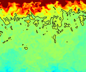
As a means of visualizing the instantaneous thermal field, figure 4 shows contours of  $c_p$ normalized by the cold wall value, which we denote $c_{p,cold}$, for the four transcritical cases. As the temperature ratio decreases, we observe a shift in location of the transition point of the Widom line towards the hot wall. Increased intensity of fluctuations in $c_p$ is visible for cases with larger temperature ratio.

Figure 4. Instantaneous contours of  $c_p$ for cases (a) TR3, (b) TR1.9, (c) TR1.4, and (d) TR1.3, normalized by $c_{p,cold}$, defined as $c_{p,w}$ at the cold wall. The half of the domain adjacent to the hot wall is shown. The $y$-axis gives $\zeta$ normalized by the channel half-height, displayed on a logarithmic scale. The solid blue line demarcates the location of the transition point of the Widom line, with $T = T_{WL}$. Contour levels and intervals are kept constant, with colour bar shown in (a).
For observations of how variations in temperature boundary conditions affect the resultant temperature field, figures 5 and 6 show temperature fluctuations near the cold and hot walls. Two different wall-normal distances are shown to capture the behaviour in both the viscous sublayer (with planes at  $\zeta ^* = 5$) and the logarithmic region (with planes at $\zeta ^* = 100$). Here, $\zeta ^*$ is the semi-local coordinate and is defined as $\zeta ^* \equiv \zeta \sqrt {\tau _w \bar {\rho }}/\bar {\mu }$. As a modification of $\zeta ^+$, $\zeta ^*$ has been used extensively in variable-property wall-bounded turbulence in order to account for the effect of local property variations on the magnitude of near-wall characteristic turbulent scales (Huang et al. Reference Huang, Coleman and Bradshaw1995).

Figure 5. Fluctuations of temperature ( $T'^{+} = T'/T_\tau$, where the prime notation denotes fluctuations from the Reynolds-averaged mean) at $\zeta ^* = 5$, for (a) TR3, cold wall, (b) TR3, hot wall, (c) TR1.3, cold wall, and (d) TR1.3, hot wall. Axes are normalized by the semi-local length scale $\bar {\mu } / \sqrt {\tau _w \bar {\rho }}$, and plots display the entire $x$–
$x$– $z$-extents of the computational domain. Contour intervals and levels are kept constant.

Figure 6. Fluctuations of temperature ( $T'^{+}$) at $\zeta ^* = 100$, for (a) TR3, cold wall, (b) TR3, hot wall, (c) TR1.3, cold wall, and (d) TR1.3, hot wall. Axes are normalized by the semi-local length scale $\bar {\mu } / \sqrt {\tau _w \bar {\rho }}$, and plots display the entire $x$–
$x$– $z$-extents of the computational domain. Colour is the same as used in figure 5.
In the viscous sublayer, the structure of the streaks is visibly distinct between the cold and hot walls. Similar qualitative characteristics in temperature fluctuations were also reported by Sengupta et al. (Reference Sengupta, Nemati, Boersma and Pecnik2017). When values are normalized by the friction temperature  $T_\tau$, we observe an increase in the relative intensity of temperature fluctuations near the hot wall at both reported $\zeta ^*$ distances for case TR1.3, due to the proximity of the hot wall temperature to $T_{WL}$.
There exists a sizeable body of literature studying near-wall velocity structures (especially for  $u'$), from which observations and associated theoretical predictions have been made. A key conclusion from previous studies is the spanwise spacing of $100$ wall plus units for near-wall streaks in $u'$ (Kline et al. Reference Kline, Reynolds, Schraub and Runstadler1967; Kim, Moin & Moser Reference Kim, Moin and Moser1987). Observations of the streak structures in temperature in figure 5 show similar spacing values of ${\sim }100$ when measured using semi-local units; these visual observations are confirmed using two-point spanwise correlations of temperature fluctuations, as plotted in figure 7. Departing from this trend is the hot wall of case TR3, which is characterized by a larger spacing approaching $400$ semi-local units. Deviations from the value of $100$ are consistent with the conclusions reached by Patel et al. (Reference Patel, Peeters, Boersma and Pecnik2015); the liquid-like structures at the cold wall tend to exhibit decreased spacing, while the gas-like structures at the hot wall tend to have increased spacing. We note also that with the high degree of correlation observed between $u'$ and $T'$ in the near-wall regime (Guo et al. Reference Guo, Yang and Ihme2018), many conclusions regarding structures in $T'$ can be compared directly with those from the near-wall $u'$ literature. Further details of transcritical velocity structures and statistics, including evidence supporting the presence of attached eddies and other comparisons with results from classical constant-property wall-bounded turbulence, are provided in Ma et al. (Reference Ma, Yang and Ihme2018).

Figure 7. Profiles of two-point spanwise correlations for temperature fluctuations,  $R_{TT}$, all at $\zeta ^* = 5$. Cold wall profiles are plotted with dashed lines, and hot wall profiles are plotted with solid lines.
For a more quantitative view of the apparent asymmetry in temperature fields, figure 8 displays probability density functions (p.d.f.s) of temperature in the viscous sublayer and in the logarithmic region. In the cold wall profiles, we observe pronounced skewness towards the hot wall temperature in the viscous sublayer. This behaviour is an indication of significant mixing of thermal energy between the two walls; similar behaviour in the density p.d.f. distributions was reported by Ma et al. (Reference Ma, Yang and Ihme2018). Profiles in the logarithmic region are less skewed (consistent with increasing isotropy in flow structures closer to the channel centre) and also display decreased overall variance compared to the viscous sublayer profiles. For the hot wall profiles, a skewness is again observed in the viscous sublayer towards the temperature of the opposite (cold) wall. However, distinct from the behaviour of the cold wall profiles, many of the hot wall profiles are observed to cluster near  $T_r = 1$ as a consequence of the proximity of $T_c$ to $T_{WL}$.

Figure 8. P.d.f.s of reduced temperature at all cases at  $\zeta ^* \simeq 5$ (solid lines) and at $\zeta ^* \simeq 100$ (dashed lines), for (a) cold wall and (b) hot wall. Hot wall profiles have been split into two subplots in order to alleviate visual congestion.
To examine the importance in fluctuations of thermodynamic quantities, figure 9 shows profiles for relative magnitudes of r.m.s. fluctuations in  $\rho$, $c_p$, $\mu$ and $\lambda$. Just as was observed for the instantaneous snapshots and the temperature p.d.f.s, a pronounced asymmetry between cold and hot wall values is observed in all cases except for case TR1, with much larger fluctuation magnitudes near the hot wall. All asymmetric cases with temperature ratio $> 1$ are also characterized by r.m.s. fluctuation values that are significantly larger than for the symmetric case TR1.

Figure 9. Profiles for r.m.s. quantities for (a) density  $\rho$, (b) constant-pressure specific heat capacity $c_p$, (c) dynamic viscosity $\mu$, and (d) thermal conductivity $\lambda$. The r.m.s. profile for a quantity $\phi$ is defined as $\phi _{rms} \equiv \sqrt { \overline {\phi '\phi '}}$. All profiles are normalized by Reynolds-averaged mean quantities.
Especially for cases with large temperature ratio (cases TR3 and TR1.9), the fluctuations in  $c_p$ are most significant and consistently exceed $50\,\%$ of the local mean value. This observation suggests the importance of capturing the behaviour of $c_p$ on characterizing the thermal boundary layer, a conclusion that was also noted by previous authors (Wan et al. Reference Wan, Zhao, Liu, Wang and Lei2020) and which we will utilize in § 3.4. We note that fluctuations in $\rho$, $\mu$ and $\lambda$ exceed $20\,\%$ of the mean value near the hot wall – with highly localized peak values for cases TR1.3 and TR1.4 – and are by no means negligible. Notably, cases TR3 and TR1.9 have fluctuation magnitudes $\gtrsim 10$% of the corresponding mean value across the majority of the channel for each of the four plotted quantities. Observations of these fluctuation profiles have important implications for the temperature characterization. With sufficiently large temperature ratio, fluctuations of all thermodynamic properties in transcritical turbulence cannot be neglected presumptively and require consideration in boundary layer modelling. This conclusion is in direct contrast to classical results. Constant-property turbulence by its nature has negligible thermodynamic fluctuation levels, and supersonic turbulent boundary layers (with significant density variation) generally follow Morkovin's hypothesis and are characterized by fluctuation magnitudes typically not exceeding 10–15 % of the mean value (Coleman, Kim & Moser Reference Coleman, Kim and Moser1995; Huang et al. Reference Huang, Coleman and Bradshaw1995).
3.2. Mean profiles
Figure 10 shows mean profiles of the decomposition of the heat flux terms into two contributions, the turbulent heat flux  $-\bar {\rho } \widetilde {v''h''}$ and the molecular heat flux $\overline {\lambda \,\partial T / \partial y}$. The tilde denotes Favre-averaged quantities, and the double prime denotes fluctuations from the Favre-averaged mean. The molecular heat fluxes exhibit similarity in behaviour among all cases. However, the same similarity is not observed for the turbulent heat fluxes, including in the near-wall thermal boundary layer (regions with large gradients in mean temperature, as can be observed in profiles of the mean temperature provided in figure 25a). The significant dissimilarity in turbulent heat flux profiles seen here was not observed in cases with lower temperature ratio values (Toki et al. Reference Toki, Teramoto and Okamoto2020).

Figure 10. Decomposition of the heat flux terms into (a) the molecular heat flux  $\overline {\lambda \,\partial T / \partial y}$ and (b) the turbulent heat flux $-\bar {\rho } \widetilde {v''h''}$. All cases are normalized by the cold wall molecular heat flux $(\overline {\lambda \,\partial T / \partial y})_{w,cold}$.
For the momentum transport, figure 11 displays the decomposition of the total mean stress into the viscous stress  $\overline {\mu \,\partial u / \partial y}$ and the Reynolds stress $-\bar {\rho } \widetilde {u''v''}$. In all cases, the profiles of viscous stress collapse well near the cold wall, while the asymmetry among different cases is evident moving towards the hot wall. It can be seen that as the temperature ratio decreases, the stress profile becomes more and more symmetric, with the Reynolds stress profile equalling zero closer to the channel centreline, and $\tau _{w,hot}$ increasing in magnitude to approach that of $\tau _{w,cold}$. Overall, similarity in the behaviour among Reynolds stress profiles is evident – a feature not observed in the turbulent heat flux profiles in figure 10.

Figure 11. Decomposition of the total momentum stress into (a) the viscous stress  $\overline {\mu \,\partial u / \partial y}$ and (b) the Reynolds stress $-\bar {\rho } \widetilde {u''v''}$. All cases are normalized by the cold wall viscous stress $(\overline {\mu \, \partial u / \partial y} )_{w,cold}$.
Despite the differences between the behaviours of the turbulent heat fluxes and Reynolds stresses, similarity is observed for the ratio of the turbulent and molecular components, as done in figure 12. The profiles provide a metric for the relative importance of each component for the momentum and energy transport as a function of  $\zeta ^*$. As observed, the dynamics of both the momentum and thermal fields are governed primarily by the molecular component for $\zeta ^* \lesssim 5$ and by the turbulent component for $\zeta ^* \gtrsim 30$. The presence of distinct spatial regimes and transport mechanisms supports early theory that led to the recognition of the logarithmic scaling of the velocity distribution, thus providing key insights towards the development of Townsend's hypothesis of equilibrium layers (Townsend Reference Townsend1961) and the Monin–Obukhov similarity theory (Monin & Obukhov Reference Monin and Obukhov1954). The observations made here, in addition to justifying the choice of $\zeta ^*$ used in studying the near-wall temperature fluctuations in § 3.1, will also be utilized for defining the extent of the temperature logarithmic region in § 3.3.

Figure 12. Ratios of turbulent and molecular components of (a) heat flux,  $-\bar {\rho } \widetilde {v''h''} / \overline {\lambda \,\partial T / \partial y}$, and (b) momentum stress, $-\bar {\rho } \widetilde {u''v''} / \overline {\mu \,\partial u / \partial y}$. Profiles are plotted against semi-local coordinate $\zeta ^*$. Cold wall profiles are plotted with dashed lines, and hot wall profiles are plotted with solid lines.
Before considering the near-wall mean temperature behaviour, it is informative to gain insight into the scales that govern the near-wall dynamics. The friction velocity and temperature are plotted in figure 13(a). From observations of  $u_\tau$ across both cold and hot walls, and in all conditions considered, variations by a factor of less than 2 are seen. The variability of the cold wall $T_\tau$ is somewhat larger, with overall variation of a factor of approximately 6, while the hot wall $T_\tau$ displays much larger variations of more than two orders of magnitude. We observe that for the hot walls, trends in both $u_\tau$ and $T_\tau$ have a noticeable non-monotonicity for cases with $T_{hot} \approx T_c$. This observation is rationalized by the significant gradients in thermodynamic properties near $T_{WL}$. Figure 13(b) compares the magnitude of the mean wall heat flux $q_w = |\lambda \,\partial T/\partial y|_w$, for each case and for the cold and hot walls. The overall trend of decreasing heat fluxes at both walls for smaller values of $T_{hot}$ is expected from observations of the mean temperature profiles in figure 25. Deviating from this trend, we observe a considerable increase in $q_{w,hot}$ for $T_{hot} / T_c = 1.03$ (corresponding to case TR1.3) that can be explained by the peak in $\lambda$ that occurs at $T_{WL}$ for weakly supercritical pressures (as observed in figure 1).

Figure 13. (a) Plots of friction velocities  $u_\tau$ and friction temperatures $T_\tau$, as a function of reduced hot wall temperature $T_{r,hot}$. Normalization in each line uses the values for case TR1. (b) Plots of magnitude of mean heat flux $q_w = | \lambda \,\partial T/\partial y|_w$ at hot and cold walls, plotted as a function of the reduced hot wall temperature $T_{r,hot}$. Normalization by the value found in case TR1 is used. In both plots, $T_{WL}$ is also plotted as a vertical dotted line.
Knowledge of the variation in characteristic scales given by figure 13 provides a foundation to investigate the temperature behaviour. Figure 14(a) shows the near-wall mean temperature profiles, normalized using the friction temperature  $T_\tau$. The cases each appear to display a region with linear slope as indication of the logarithmic region; this observation is also substantiated using the diagnostic function plotted in figure 14(b). If friction quantities by themselves were sufficient to describe the mean temperature dynamics, then all profiles would collapse into a single curve and thus satisfy a universal temperature law of the wall, in the form as presented by (1.1) but with $\zeta ^*$ replacing $\zeta ^+$. While this is not the case, the observed profiles provide insight into the ability of $T_\tau$ to describe accurately the near-wall scales for the temperature dynamics. The cold wall profiles collapse more tightly – with similar log region slopes and amount of vertical shift – than the hot wall profiles do; this indicates that $T_\tau$ at the cold walls performs relatively well as a normalization quantity. This good collapse of the cold wall profiles is expected; profiles at the cold walls are more similar in nature to classical constant-property results, with comparatively less effect of near-wall property gradients on the mean flow. In contrast, the hot wall profiles of cases TR3 and TR1.9 display noticeably smaller slopes and are shifted vertically downwards compared to the cold wall profiles and to all other hot wall profiles. This suggests that near the hot wall, $T_{\tau,TR3}$ and $T_{\tau,TR1.9}$ overestimate the true near-wall temperature scales. The opposite conclusion can be made for the hot wall profiles of TR1.3 and TR1.25; the log regions in these cases have slope values that are too large and profiles that are shifted vertically upwards.

Figure 14. Profiles for (a) normalized mean temperature  $\bar {\theta }^+$, and (b) the log law diagnostic function $\zeta ^* \,{\rm d} \bar {\theta }^+ / {\rm d} \zeta ^*$. For each profile, the diagnostic function approaches a constant value in the logarithmic region, corresponding to $1 / \kappa _T$ in (1.1). Dashed lines indicate cold wall profiles, and solid lines indicate hot wall profiles. All 12 curves (6 cases with 2 walls each) are displayed. Profiles are plotted versus the semi-local coordinate $\zeta ^*$.
These profiles of near-wall mean temperature serve as a baseline for the characterization efforts that follow. Additional mean profiles to illustrate the flow are provided in Appendix B.
3.3. Assessment of previous mean temperature theoretical work
As discussed in § 1, the mean temperature behaviour of the viscous sublayer is well characterized. For completeness, we show these profiles in § 3.2. In this subsection, we focus on the quantitative assessment of the performance of previous transformations from literature in characterizing the logarithmic region of the mean temperature profile for our simulations. Note that while we included case TR1 in plots and discussions up to this point as a reference case, we will not consider it for purposes of characterization and modelling.
Before beginning the assessment, the boundaries of the temperature log region must be defined properly. For the velocity log law, the log region is defined as being between  $\zeta ^* > 30$ and $\zeta /L_y < 0.3$; these bounds have been well-validated using data from both computational and experimental investigations (Pope Reference Pope2000).
The lower bound value of  $\zeta ^* = 30$ for the velocity log law is chosen based on observations from past studies that the direct effect of the molecular viscosity on the total viscous stress is negligible in the region further than ${\sim }30$ viscous length scales from the wall (Pope Reference Pope2000). From the observations and discussion associated with figure 12, it is seen that both the viscous stress and the molecular heat flux are negligible for our cases for $\zeta ^* \gtrsim 30$. Thus we choose to use the same value of $\zeta ^* = 30$ for the lower bound of the temperature log region. Observations of figure 14 support this choice for the cases under investigation, with a region of linear slope for all cases beginning at $\zeta ^* \approx 30$ and extending away from the wall.
For the upper bound of the temperature log region, modification of the velocity log law criterion ( $\zeta /L_y < 0.3$) is necessary. The criterion from the velocity log law stems from the fact that $\zeta = L_y$ is the location of the maximum of $\bar {u}$ in a symmetric channel. In our current investigation, it can be seen in figure 25(c) that the peak in $\bar {u}$ deviates significantly from $\zeta = L_y$ for several cases, making $\zeta = L_y$ an ill-suited choice in our current investigation. Instead, we choose $L_{y,max(\bar {u})}$ – the distance from the wall to the location of maximum $\bar {u}$ – as the relevant length scale for each case, as was also used to calculate $Re_{\tau, max(\bar {u})}$ in table 1. The modified upper bound for the temperature log region is thus $\zeta / L_{y,max(\bar {u})} < 0.3$. Values for the location of this temperature log region upper bound are provided in table 3.
Table 3. Distance from wall to location of maximum mean streamwise velocity,  $L_{y,max(\bar {u})} / L_y$, and the corresponding location of the upper bound of the temperature log region, $\zeta = 0.3\, L_{y,max(\bar {u})}$, in semi-local units.

With our clarification of the boundaries for the temperature log region, we proceed by reviewing previous transformations from literature. We quantify the performance of a transformation by (1) how the slopes of the temperature log region differ among cases, and (2) how well the shift parameter of the temperature log region is characterized. Here, the shift parameter of the temperature log region is defined to be the value of the transformed temperature at  $\zeta ^* = 30$, and can be interpreted as a measure of the vertical variation in the log region of the transformed temperature.
Note that the presented integrals are of the form
 \begin{equation} \int_{d_1}^{d_2} \psi(\varphi) \, {\rm d} \varphi, \end{equation}
with  $d_1$ and $d_2$ being the limits of the interval of integration and $\psi$ being the integrand. Throughout, $\varphi$ is used as an arbitrary dummy variable to represent a point within the interval of integration, with $\varphi \in [ d_1, d_2 ]$.
The first transformation from literature is a scalar analogy of the velocity van Driest (VD) transformation. Known as the temperature van Driest transformation, this transformation is given as
 \begin{equation} \bar{\theta}_{VD}^+{=} \int_0^{\bar{\theta}^+} \sqrt{\frac{\bar{\rho}}{\rho_w}}\, \frac{\overline{c_p}}{c_{p,w}} \,{\rm d} \varphi. \end{equation}
A version with constant  $c_p$ was discussed in Patel et al. (Reference Patel, Boersma and Pecnik2017), and a formulation with variable $c_p$ was discussed in Wan et al. (Reference Wan, Zhao, Liu, Wang and Lei2020). Both studies report unsatisfactory collapse of the temperature profiles, and each study attributes this result to the influence of near-wall property variations that are unaccounted for by the transformation. We plot the results of this transformation for our data in figure 15(a) and note that, in addition to the variation in the log region shift parameter, the slopes among different cases vary across a wide range. It is evident that accounting only for variations in $\bar {\rho }$ and $\overline {c_p}$ is not sufficient to fully describe the mean temperature profile. In contrast, Ma et al. (Reference Ma, Yang and Ihme2018) demonstrated good agreement with the established velocity log law correlation when using the velocity van Driest transformation on the $\bar {u}$ profile.

Figure 15. Profiles of (a) the temperature van Driest transformation, (b) the transformation proposed by Toki et al. (Reference Toki, Teramoto and Okamoto2020), and (c) the extended van Driest transformation proposed by Patel et al. (Reference Patel, Boersma and Pecnik2017) and Wan et al. (Reference Wan, Zhao, Liu, Wang and Lei2020). In the left-hand panels, dashed lines indicate cold wall profiles, and solid lines indicate hot wall profiles. Log region slopes and shift parameters are also plotted for each transformation. For each transformed profile, log region slope values are determined using the slope of the line of best fit through the temperature log region, and the shift parameter is given by the value of the profile at  $\zeta ^* = 30$ ( $\zeta ^+ = 30$ for the Toki et al. (Reference Toki, Teramoto and Okamoto2020) transformation).
A second transformation proposed by Toki et al. (Reference Toki, Teramoto and Okamoto2020) is derived using the mixing length hypothesis for both momentum and energy and also by assuming linear shear stress and heat flux. This transformation is written as
 \begin{equation} \tilde{\theta}_{Toki}^{*} = \int_0^{\tilde{\theta}^+} \sqrt{ \frac{\bar{\rho}}{\rho_w} }\, \frac{\widetilde{c_p}}{c_{p,w}} \,{\rm d} \varphi. \end{equation}
The results for this transformation are provided in figure 15(b). The Toki transformation shows a slight improvement over the van Driest transformation when observing the collapse of the slope. However, significant deviations from the reported slope value of  $2.8$ (provided in Toki et al. Reference Toki, Teramoto and Okamoto2020) are seen, especially for the hot wall of case TR3.
We now analyse the behaviour of the extended van Driest (eVD) transformation, first proposed by Patel et al. (Reference Patel, Boersma and Pecnik2017) and later extended to variable  $c_p$ conditions by Wan et al. (Reference Wan, Zhao, Liu, Wang and Lei2020). The derivation of the transformation begins from the low-Mach energy equation, with a final expression written as
 \begin{equation} \bar{\theta}_{eVD}^* = \int_0^{\zeta^*} \dfrac{1}{\dfrac{\alpha_t}{\bar{\mu}} + \dfrac{1}{Pr^*}} \,{\rm d}\varphi, \end{equation}
where the turbulent eddy conductivity is defined to be  $\alpha _t = (-\bar {\rho } \widetilde {v'' \theta ''}) / ({\rm d} \bar {\theta }/{{\rm d}y})$. The local Prandtl number is defined as $Pr^* = Pr_w (\overline {c_p} / c_{p,w}) (\bar {\mu } / \mu _w) / (\bar {\lambda } / \lambda _w) = \overline {c_p} \, \bar {\mu } / \bar {\lambda }$ and is plotted and discussed in Appendix B. Notably, while (3.2) and (3.3) are direct integral transformations for temperature, (3.4) is a spatial integral. The results of this transformation for our data are provided in figure 15(c). Though significant improvement in the collapse of the slope is achieved when compared to previous models, we observe a large spread in slope values of ${\sim }\pm 0.8$ (corresponding to an uncertainty percentage of approximately ${\pm }25\,\%$ from an average value of ${\sim }3.3$). Increasingly large slope values are found for the hot wall of cases with larger temperature ratios, with an especially large value for the hot wall of case TR3. This difficulty in collapse indicates that the governing physical processes of the near-wall temperature dynamics are not sufficiently accounted for at higher temperature ratios. Our current study seeks to address this issue in § 3.4.
An additional feature of the extended van Driest transformation is a mathematical description of the log region shift parameter by decomposing (3.4) into two portions:
 \begin{equation} \bar{\theta}_{eVD}^* = \bar{\theta}_{\mathcal{T},eVD}^* + \bar{\theta}_{\mathcal{P},eVD}^*, \quad \text{with} \ \bar{\theta}_{\mathcal{T},eVD}^* = \int_0^{\zeta^*} \frac{1}{\left( \dfrac{\alpha_t}{\bar{\mu}} + 1 \right) } \,{\rm d} \varphi. \end{equation}
One portion,  $\bar {\theta }_{\mathcal {T},eVD}^*$, sets $Pr^* = 1$ to remove variations in the viscous sublayer (and thus remove variation in the log region shift parameter) to isolate the log region slope. A second portion, $\bar {\theta }_{\mathcal {P},eVD}^*$, captures the different log region shift parameters of each case by removing the effect of the log region slope. Figure 16 shows this decomposition. With this formulation, the log region shift parameters given in figure 15(c) can be found by adding the asymptotic values of $\bar {\theta }_{\mathcal {P},eVD}^*$ to the log region shift parameter of $\bar {\theta }_{\mathcal {T},eVD}^*$. We expand upon this decomposition in our model development in § 3.4.

Figure 16. Profiles of the decomposition of the extended van Driest transformation proposed by Patel et al. (Reference Patel, Boersma and Pecnik2017) and Wan et al. (Reference Wan, Zhao, Liu, Wang and Lei2020) into (a) the portion that characterizes the log region slope,  $\bar {\theta }_{\mathcal {T},eVD}^*$, and (b) the portion that characterizes the log region shift parameter, $\bar {\theta }_{\mathcal {P},eVD}^*$. Dashed lines indicate cold wall profiles, and solid lines indicate hot wall profiles.
In these presented transformations, we observe significant non-universality in the value of log region slopes obtained. Difficulties in collapsing the slope values are especially pronounced near the hot wall for cases TR3 and TR1.9 (with  $T_{r,hot} = 2.58$ and $1.51$, respectively); these coincide with large values of $T_\tau$ and $q_w$, as shown in § 3.2 through the discussion associated with figure 13. We observe deviations from the general trend of hot wall slopes for cases TR1.3 and TR1.25 as a result of the proximity of the transition point of the Widom line; however, we do not observe the same degree of difficulty in collapse of slopes as in the hot walls of cases TR3 and TR1.9. Specifically for the log region shift parameter, a common theme that we observe is the larger shift parameter values found near the hot walls for cases TR1.3 and TR1.4 (with $T_{r,hot} = 1.03$ and $1.11$, respectively). This common observation can be rationalized by the proximity of these cases to $T_{WL}$ and the corresponding peak $Pr^*$ that occurs at this temperature. We note that in the transformations presented in this section, the log region shift parameter is either not predicted by the proposed mathematical transformation (for the van Driest and Toki transformations) or characterized a posteriori using the transformed DNS profiles (for the extended van Driest transformation).
3.4. Mean temperature characterization and modelling
From observations of the performance of currently available transformations in § 3.3, an improved transformation for the near-wall mean temperature profile would provide a characterization of the log region slope with higher accuracy. An improved transformation would also contain a predictive model for the log region shift parameter. If the log region shift parameter could be determined using only values known a priori, then the details of the temperature profile in the log region can be quantitatively predicted beforehand, increasing the applicability of the transformation to turbulence modelling. These are the goals that motivate our proposed transformation, which we derive next.
To consider the entire set of relevant physical processes, we begin with the energy equation (2.1c); after subtracting the transport of kinetic energy and then averaging over time and over homogeneous directions, we obtain
 \begin{equation} - \bar{\rho} \widetilde{v''h''} + \overline{\lambda\,\frac{{\rm d} \theta}{{\rm d} \zeta}} + \int_{0}^{\zeta} \overline{u_i\,\frac{\partial p}{\partial x_i}} \,{\rm d} \varphi + \int_{0}^{\zeta} \overline{\tau_{ij}\,\frac{\partial u_i}{\partial x_j}} \,{\rm d} \varphi \equiv \bar{q}, \end{equation}
where  $q$ represents the total heat flux. Note that in this equation, the turbulent heat flux term $- \bar {\rho } \widetilde {v''h''}$ and the molecular heat flux term $\overline {\lambda \,{\rm d} \theta / {\rm d} \zeta }$ are present, as well as two additional terms: the pressure work term $\int _{0}^{\zeta } \overline { u_i\,\partial p / \partial x_i } \,{\rm d}\varphi$ and the viscous dissipation of kinetic energy $\int _{0}^{\zeta } \overline {\tau _{ij}\,\partial u_i / \partial x_j } \,{\rm d}\varphi$. These integrals are evaluated from the wall to the desired $\zeta$ location. Notably, these last two terms are neglected by the energy equation of the low-Mach limit of the Navier–Stokes equations.
In simplifying the energy equation, we make two assumptions. The first is that the fluctuating molecular heat flux is negligible,  $|\bar {\lambda } \, {\rm d} \bar {\theta } / {\rm d} \zeta | \gg | \overline {\lambda ' \, {\rm d} \theta ' / {\rm d} \zeta }|$. Although observations of the r.m.s. fluctuations as seen in figure 9 have shown that such fluctuations of thermodynamic properties (including $\lambda$) can be significant, figure 17(a) shows that the contributions of the fluctuating heat flux are small when normalized by $\bar {q}$. Additionally and more importantly, the profiles decay to $0$ for $\zeta ^* > 30$. Because our primary focus is the characterization of the temperature log region, this first assumption is justified, and we approximate the molecular heat flux term as
 \begin{equation} \overline{\lambda\,\frac{{\rm d} \theta}{{\rm d} \zeta}} \approx \bar{\lambda}\,\frac{{\rm d} \bar{\theta}}{{\rm d} \zeta}. \end{equation}
Figure 17. Profiles of (a) fluctuating molecular heat flux  $\overline {\lambda ' \,{\rm d} \theta ' / {\rm d} \zeta }$, (b) pressure work $\int _{0}^{\zeta } \overline {u_i\,\partial p / \partial x_i} \,{\rm d} \varphi$, and (c) viscous dissipation of kinetic energy $\int _{0}^{\zeta } \overline {\tau _{ij}\,\partial u_i / \partial x_j} \,{\rm d} \varphi$. All terms have been normalized by the total mean heat flux $\bar {q}$, as defined in (3.6). Dashed lines indicate cold wall profiles, and solid lines indicate hot wall profiles.
As a second simplifying approximation, we neglect the pressure work term while keeping the viscous dissipation of kinetic energy. Figure 17(b) shows the pressure work, and figure 17(c) shows the viscous dissipation of kinetic energy. When assessing the absolute value of the relative magnitude across all cases, the pressure work is two orders of magnitude smaller than the other terms in consideration in figure 17, and thus does not provide a significant contribution to the overall heat flux. In contrast, the viscous dissipation contributes 5–10 % of the overall heat flux in certain cases. These contributions are most significant in the temperature log region for  $\zeta ^* > 30$. We thus neglect the fluctuating molecular heat flux and the pressure work but keep the viscous dissipation. With this simplification, we rewrite (3.6) as
 \begin{equation} - \bar{\rho} \widetilde{v''h''} + \bar{\lambda}\,\frac{{\rm d} \bar{\theta}}{{\rm d} \zeta} + \int_{0}^{\zeta} \overline{\tau_{ij}\,\frac{\partial u_i}{\partial x_j}} \,{\rm d} \varphi \approx \bar{q}. \end{equation}
Normalizing each term with the wall heat flux  $q_w = \rho _w u_\tau c_{p,w} T_\tau$ and rearranging leads to
 \begin{equation} \left( \frac{\alpha_t}{\bar{\mu}} + \frac{1}{Pr^*} \right) \frac{L_y}{Re_\tau^*} \sqrt{ \dfrac{\bar{\rho}}{\rho_w} }\,\frac{\overline{c_p}}{c_{p,w}}\,\frac{{\rm d} \bar{\theta}^+ }{{\rm d}\zeta} \approx \frac{\bar{q} - \displaystyle\int_{0}^{\zeta} \overline{\tau_{ij}\,\dfrac{\partial u_i}{\partial x_j}} \,{\rm d}\varphi}{q_w}, \end{equation}
where the turbulent eddy conductivity  $\alpha _t$, accounting for enthalpy fluctuations, is defined as
 \begin{equation} \alpha_t ={-}\frac{\bar{\rho} \widetilde{v''h''}}{\overline{c_p}\,\dfrac{{\rm d} \bar{\theta}}{{\rm d}y}}. \end{equation}
The potential of (3.9) in collapsing the  $\bar {\theta }$ profile rests on how well the quantity
 \begin{equation} \frac{{\rm d} \bar{\theta}^*}{{\rm d} \zeta^*} \equiv \frac{L_y}{Re_\tau^*} \sqrt{ \frac{\bar{\rho}}{\rho_w} }\,\frac{\overline{c_p}}{c_{p,w}}\,\frac{{\rm d} \bar{\theta}^+ }{{\rm d}\zeta} \end{equation}
collapses among different cases as a function of  $\zeta ^*$. Here, we introduce the ${\rm d} \bar {\theta }^* / {\rm d} \zeta ^*$ label following the notation used by Patel et al. (Reference Patel, Boersma and Pecnik2017). Following the definition in (3.11), we can rearrange the terms in (3.9) to obtain
 \begin{equation} \dfrac{{\rm d} \bar{\theta}^*}{{\rm d} \zeta^*} \approx \dfrac{\bar{q} - \displaystyle\int_{0}^{\zeta} \overline{\tau_{ij}\,\dfrac{\partial u_i}{\partial x_j}} \,{\rm d} \varphi}{q_w}\, \dfrac{1}{\dfrac{\alpha_t}{\bar{\mu}} + \dfrac{1}{Pr^*}} = \dfrac{1}{C_1}\, \dfrac{1}{\dfrac{\alpha_t}{\bar{\mu}} + \dfrac{1}{Pr^*}}, \end{equation}
as an approximate representation of (3.11), which will be used to develop a mathematical transformation to model the mean temperature. Here,  $C_1$ is given as
 \begin{equation} C_1 = \frac{q_w}{\bar{q} - \displaystyle\int_{0}^{\zeta} \overline{\tau_{ij}\,\dfrac{\partial u_i}{\partial x_j}} \,{\rm d} \varphi}. \end{equation}
 The profiles of  ${\rm d} \bar {\theta }^* / {\rm d} \zeta ^*$, as defined in (3.11), are plotted in figure 18(a). We observe significant spread in magnitudes of profiles among cases; in the temperature log region (defined by the discussion in § 3.3), relative magnitudes of cases span a factor of up to 3. Notably, the magnitude of profiles for the hot walls of cases TR3 and TR1.9 are consistent outliers. To correct for these observed discrepancies among profiles, we introduce two correction factors to be multiplied by ${\rm d} \bar {\theta }^* / {\rm d} \zeta ^*$ as given in (3.11):
 \begin{equation} \frac{{\rm d} \bar{\theta}^*}{{\rm d} \zeta^*}\,C_1 C_2, \end{equation}
with  $C_1$ as given by (3.13) and $C_2$ given as
 \begin{equation} C_2 = \frac{1}{\overline{c_p}}\,\frac{{\rm d} \bar{h}}{{\rm d} \bar{\theta}}. \end{equation}
As seen in figure 18(b), these two correction terms achieve significant improvement in the collapse of  ${\rm d} \bar {\theta }^* / {\rm d} \zeta ^*$, when compared with the uncorrected values in figure 18(a). The term $C_1$ corrects for the observed variation in total heat flux across cases. The term $C_2$ corrects for an implicit approximation made by the eddy conductivity definition in (3.10) – a more appropriate eddy conductivity would use the enthalpy gradient ${\rm d} \bar {h} / {{\rm d}y}$, instead of $\overline {c_p}\, {\rm d} \bar {\theta } / {{\rm d}y}$, in the denominator of the definition of $\alpha _t$. Note that the specific enthalpy differential for a real fluid is a function of two independent state variables – such as $T$ and $p$ – and can be written as
 \begin{equation} h = h(T,p) \rightarrow {\rm d}h = \left( \frac{\partial h}{\partial T} \right)_p \,{\rm d}T + \left( \frac{\partial h}{\partial p} \right)_T \,{\rm d}p = c_p \,{\rm d}T + \left( \frac{\partial h}{\partial p} \right)_T \,{\rm d}p. \end{equation}
Employing  ${\rm d}h = T\,{\rm d}s + (1/\rho )\,{\rm d}p$ leads to
 \begin{equation} \left( \frac{\partial h}{\partial p} \right)_T = T \left( \frac{\partial s}{\partial p} \right)_T + \frac{1}{\rho} ={-}T \left( \frac{\partial (1/\rho)}{\partial T} \right)_p + \frac{1}{\rho}, \end{equation}
where the Maxwell relation
 \begin{equation} \left( \frac{\partial s}{\partial p} \right)_T ={-} \left( \frac{\partial (1/\rho) }{\partial T}\right)_p \end{equation}
has been used. Substituting (3.17) into (3.16) leads to
 \begin{equation} {\rm d}h = c_p \,{\rm d}T + \frac{1}{\rho} \left(1 + \frac{T}{\rho} \left( \frac{\partial \rho}{\partial T} \right)_p \right) \,{\rm d}p, \end{equation}
thus showing that  ${\rm d}h \neq c_p \,{\rm d} \theta$ for a real fluid.

Figure 18. Profiles of (a)  ${\rm d} \bar {\theta }^* / {\rm d} \zeta ^*$, and (b) $C_1 C_2 \,{\rm d} \bar {\theta }^* / {\rm d} \zeta ^*$. Dashed lines indicate cold wall profiles, and solid lines indicate hot wall profiles.
The combination of  $C_1$ and $C_2$ has demonstrated their ability to provide a physics-motivated collapse of the profiles of (3.11). Our goal is to achieve an accurate transformation to represent (3.11), and in turn represent the mean temperature profile. Given the success of the correction factor procedure, we apply the same procedure to the approximate representation for ${\rm d} \bar {\theta }^* / {\rm d} \zeta ^*$ as given by (3.12) and obtain
 \begin{equation} \dfrac{C_2}{ \dfrac{\alpha_t}{\bar{\mu}} + \dfrac{1}{Pr^*} } = \dfrac{\dfrac{1}{\overline{c_p}}\, \dfrac{{\rm d} \bar{h}}{{\rm d} \bar{\theta}}}{ \dfrac{\alpha_t}{\bar{\mu}} + \dfrac{1}{Pr^*} }, \end{equation}
which serves as the basis of the integrand of our proposed transformation to represent the mean temperature profile.
With these corrections in place, we can now define a temperature transformation in the near-wall region by integrating (3.20) to obtain
 \begin{equation} \bar{\theta}^* \equiv \int_0^{\zeta^*} \dfrac{\dfrac{1}{\overline{c_p}}\,\dfrac{{\rm d} \bar{h}}{{\rm d} \bar{\theta}}}{ \dfrac{\alpha_t}{\bar{\mu}} + \dfrac{1}{Pr^*} } \,{\rm d} \varphi. \end{equation}
 Profiles of the full transformation  $\bar {\theta }^*$ as given in (3.21) are plotted in figure 19, along with the slope and shift parameter that best fit the logarithmic region of the profile. The slopes are all clustered nicely around a mean value of ${\sim }3.2$ (with a reduced range of ${\sim }\pm 0.56$ among all cases, corresponding to an improved uncertainty percentage range of approximately ${\pm }18\,\%$).

Figure 19. (a) Profiles of the full transformation, as given in (3.21). Dashed lines indicate cold wall profiles, and solid lines indicate hot wall profiles. (b) Slopes and shift parameters of each case, plotted against the temperature at the hot wall. For each transformed profile, log region slope values are determined using the slope of the line of best fit through the temperature log region, and the shift parameter is given by the value of the profile at  $\zeta ^* = 30$.
We observe a shift in the log region shift parameter that is seen in previous models and can be explained by  $Pr^*$ effects. Borrowing the procedure of Patel et al. (Reference Patel, Boersma and Pecnik2017) and Wan et al. (Reference Wan, Zhao, Liu, Wang and Lei2020), the final transformation $\bar {\theta }^*$ can be decomposed into two separate terms, as
 \begin{equation} \bar{\theta}^* = \bar{\theta}_{\mathcal{T}}^* + \bar{\theta}_{\mathcal{P}}^*. \end{equation}
One term,  $\bar {\theta }_{\mathcal {T}}^*$, characterizes the slope of the log region and assumes unity $Pr^*$:
 \begin{equation} \bar{\theta}_{\mathcal{T}}^* = \int_0^{\zeta^*} \dfrac{\dfrac{1}{\overline{c_p}}\,\dfrac{{\rm d} \bar{h}}{{\rm d} \bar{\theta}}}{ \dfrac{\alpha_t}{\bar{\mu}} + 1 } \,{\rm d} \varphi. \end{equation}
The second term,  $\bar {\theta }_{\mathcal {P}}^*$, contains effects of variable $Pr^*$ on the shift parameter of the log region, and is written as
 \begin{equation} \bar{\theta}_{\mathcal{P}}^* = \int_0^{\zeta^*} \left( \dfrac{ \dfrac{1}{\overline{c_p}}\,\dfrac{{\rm d} \bar{h}}{{\rm d} \bar{\theta}} }{ \dfrac{\alpha_t}{\bar{\mu}} + \dfrac{1}{Pr^*}} - \dfrac{ \dfrac{1}{\overline{c_p}}\,\dfrac{{\rm d} \bar{h}}{{\rm d} \bar{\theta}} }{ \dfrac{\alpha_t}{\bar{\mu}} + 1} \right) \,{\rm d} \varphi. \end{equation}
Figure 20(a) shows profiles of  $\bar {\theta }_{\mathcal {T}}^*$; with the removal of variations in log region shift parameter, we observe good collapse among profiles. To provide a modelled profile using an empirical fit, we integrate an ODE-based wall model equation for near-wall mean temperature (as an analogy of the near-wall mean velocity model equation of Kawai & Larsson Reference Kawai and Larsson2012):
 \begin{equation} \frac{{\rm d} \bar{\theta}_{\mathcal{T}}^* }{{\rm d}\zeta^*} = \frac{1}{1 + l_T^*}, \end{equation}
where the mixing length parameter  $l_T^*$ is given by
 \begin{equation} l_T^* = \frac{1}{\kappa_T^*}\,\zeta^* \left( 1 - \exp \left[ - \left( \frac{\zeta^*}{A} \right)^{2/b} \right] \right)^b. \end{equation}
Parameter choices used in figure 20(a) to best describe the data are  $\kappa _T^* = 2.90$, $A = 23$ and $b = 1$. Figure 20(b) shows profiles of $\bar {\theta }_{\mathcal {P}}^*$. The observation that $\bar {\theta }_{\mathcal {P}}^*$ reaches an asymptotic value for $\zeta ^* \gtrsim 30$ indicates that the variation in the shift parameter of the log region for $\bar {\theta }^*$ comes nearly exclusively from variations in ${\rm d} \bar {\theta }_{\mathcal {P}}^* / {\rm d} \zeta ^*$ for $\zeta ^* \lesssim 30$ (in the viscous sublayer and in the buffer layer). The log region shift parameter for $\bar {\theta }^*$ can now be described as the sum of (1) the log region shift parameter value for $\bar {\theta }_{\mathcal {T}}^*$, which is ${\sim }14$ for all cases, and (2) $\bar {\theta }_{\mathcal {P}}^* (\zeta ^* = 30)$.

Figure 20. Profiles of (a)  $\bar {\theta }_{\mathcal {T}}^*$, where the fitted curve is per (3.25), and (b) $\bar {\theta }_{\mathcal {P}}^*$. Dashed lines indicate cold wall profiles, and solid lines indicate hot wall profiles.
As mentioned previously, the ability to predict the shift parameter of the log region for  $\bar {\theta }^*$ has direct utility in turbulence modelling. In analysing the distribution of values for $\bar {\theta }_{\mathcal {P}}^* (\zeta ^* = 30)$, we observe a significant increase for wall temperatures near $T_{WL}$. We make the following observations and approximations.
(i) From the expression for $\bar {\theta }_{\mathcal {P}}^*$ given in (3.24), the value of ${\rm d} \bar {\theta }_{\mathcal {P}}^* / {\rm d}\zeta ^*$ at the wall ($\zeta ^* = 0$) can be estimated for all cases to be $Pr_w - 1$.
(ii) Given that
$Pr$ reaches a maximum at $T = T_{WL}$, an estimated theoretical maximum value of ${\rm d} \bar {\theta }_{\mathcal {P}}^* / {\rm d}\zeta ^*$ for $\zeta ^* = 0$ is $(Pr_{WL} - 1)$, where $Pr_{WL}$ is the value of $Pr$ evaluated at $T = T_{WL}$. A reasonable estimate for the integral of ${\rm d} \bar {\theta }_{\mathcal {P}}^* / {\rm d}\zeta ^*$ from $\zeta ^* = 0$ to $\zeta ^* = 30$ to obtain $\bar {\theta }_{\mathcal {P}}^* (\zeta ^* = 30)$ is $3 (Pr_{WL} - 1)$.(iii) At values of
$|T_w - T_{WL}| / T_{WL}$ exceeding unity, $Pr$ will approach the same value as found in an ideal gas, which we denote as $Pr_{ig}$. In this regime, a reasonable estimate for the integral of ${\rm d} \bar {\theta }_{\mathcal {P}}^* / {\rm d}\zeta ^*$ from $\zeta ^* = 0$ to $\zeta ^* = 30$ to obtain $\bar {\theta }_{\mathcal {P}}^* (\zeta ^* = 30)$ is $5 (Pr_{ig} - 1)$.


Figure 21, developed using these observations, shows our prediction of the values of  $\bar {\theta }_{\mathcal {P}}^* (\zeta ^* = 30)$, along with an exponential function that best fits the data. Although the exact value of the log region shift parameter would still require the evaluation of the expression in (3.24), this approximation provides a framework to estimate the value quantitatively with reasonable accuracy.

Figure 21. Values of  $\bar {\theta }_{\mathcal {P}}^* (\zeta ^* = 30)$, normalized by a maximum value, $3 (Pr_{WL} - 1)$, plotted against normalized temperature coordinate $|T_w - T_{WL}| / T_{WL}$. The fitted curve is an exponential function of the form $x_2 = a_1 \exp (-a_2 T_{input}^*) + a_3$, where $T_{input}^*$ and $x_2$ are the $x$- and $y$-axis quantities of the plot, respectively. Parameter values used to generate the curve shown are $a_1 = 1.06$, $a_2 = 4.5$ and $a_3 = -0.06$.
This concludes the derivation of our mean temperature transformation. Previous formulations began their model development by starting off with one or more simplifying assumptions – namely the low-Mach equations and hypotheses of linear heat flux/stress – that restrict the applicability and performance of the transformations. Instead, we consider, from the outset, all possible physical processes allowed by the energy equation.
In assessment of performance, our transformation offers reduced uncertainty in the value of log region slope. Note that the current transformation improves the collapse of the slope near the hot walls for cases TR3 and TR1.9 – cases that previous transformations have struggled with, likely due to the presence of steeper gradients in mean temperature (figure 25a), larger relative values of fluctuations (figure 9), real fluid considerations for the enthalpy, and larger heat flux and friction temperature values (figure 13). Additionally, we have presented a methodology to estimate the log region shift parameter a priori, thus providing a quantitative, predictive view for the near-wall mean temperature profile.
4. Conclusions
The results of DNS calculations for a fully developed transcritical turbulent channel flow at a reduced pressure  $p_r = 1.14$ are presented. The ratio of wall temperatures of the cases is varied up to a value of 3, resulting in four transcritical and two non-transcritical cases with density ratios of up to $O(20)$. For the transcritical cases, the asymmetric thermodynamic behaviour of the liquid-like and gas-like regimes, as well as the direct influence of the Widom line, strongly interact with the turbulence dynamics and heat transfer in the near-wall regime. The impact of the transcritical thermodynamics is also evident through a number of modifications to flow structures and statistics.
(i) Compared to classical boundary layer trends, the spanwise spacing of temperature structures is widened in the gas-like regime and contracted in the liquid-like regime.
(ii) Probability distributions of temperature fluctuations exhibit increased skewness, which is indicative of significant mixing between the hot and cold walls.
(iii) Enhanced turbulent fluctuations in the transcritical thermal field and in thermodynamic quantities are observed, with r.m.s. fluctuation levels reaching
${>}90\,\%$ of $\overline {c_p}$ and ${>}25\,\%$ of $\bar {\rho }$, $\bar {\mu }$ and $\bar {\lambda }$. Large turbulent magnitudes are seen especially near the hot wall as a consequence of the proximity of the transition point of the Widom line.


Although profiles of the momentum and thermal transport appear disparate in nature, the molecular and turbulent transport were each found to be the dominant mechanism in the same wall-normal region of both fields.
The previous characterization efforts for the near-wall mean temperature profile are examined, along with a quantitative assessment of their strengths and weaknesses. Difficulty in consistently characterizing the near-wall temperature dynamics is seen in conditions with large density ratios and the associated steep gradients in mean temperature, larger relative fluctuation magnitudes, real fluid considerations for the enthalpy, and increased heat flux and friction quantity magnitudes. In certain conditions, the viscous dissipation of kinetic energy is also found to be a non-negligible portion of the total heat flux. To address these findings, a new characterization is introduced and derived systematically. Results demonstrate improved collapse in the log region slope to within  ${\pm }18\,\%$ uncertainty. Following the procedure proposed by Patel et al. (Reference Patel, Boersma and Pecnik2017), the full transformation is split into two component terms. The first term, $\bar {\theta }_\mathcal {T}^*$, characterizes the log region slope and collapses well among all cases into a single, near-universal profile. The second term, $\bar {\theta }_\mathcal {P}^*$, characterizes the non-universal log region shift parameter that deviates significantly for different operating conditions. After a predictive framework is developed that models the log region shift parameter using the results of $\bar {\theta }_\mathcal {P}^*$, the near-wall mean temperature profile in the logarithmic region can be described fully as a modelled analytical profile. This theoretical framework, by capturing the impact of select physical processes on characterizing the turbulence dynamics, thus guides the development of more accurate turbulence models for wall-bounded transcritical flows.
Acknowledgements
J.G. would like to thank K.P. Griffin and N. Singh for helpful discussions.
Funding
This work was supported by the Stanford Graduate Fellowship through a Charles H. Kruger Graduate Fellowship (J.G.) and the Department of Energy Office of Science with award number DE-SC0021129 (J.G., M.I.). Resources supporting this work were provided by the NASA High-End Computing (HEC) Program through the NASA Advanced Supercomputing (NAS) Division of Ames Research Center (ARC).
Declaration of interests
The authors report no conflict of interest.
Appendix A. Grid resolution
To illustrate the grid resolution for the cases, we present grid analysis studies for  $\Delta x$ and $\Delta y$. Typical channel DNS resolution requirements are approximately equivalent for $x$ and $z$;
$z$;  $\Delta x > \Delta z$ in our set-up, so conclusions in our study about the resolution for $\Delta x$ are also applicable to requirements on $\Delta z$. Grid resolutions for each case are calculated and discussed for three different length scales: (1) Kolmogorov length scales $\eta _u$, (2) thermal Kolmogorov length scales $\eta _T$, and (3) viscous wall units (plus units).
Grid spacing curves for the Kolmogorov lengths are presented in figure 22 for  $\eta _u$ and $\eta _T$. Here, $\eta _u = ( \nu ^3 / \bar {\epsilon } )^{1/4}$ for the Kolmogorov length scale with turbulent dissipation rate $\bar {\epsilon } = \overline {\tau _{ij} \, \partial u_i'' / \partial x_j } / \bar {\rho }$, and $\eta _T = \eta _u / \sqrt {\overline {Pr}}$ for the thermal Kolmogorov length scale. Across the majority of the channel, $\Delta x \approx (2.5\text {--}7.0) \eta _u \approx (3.5\text {--}11) \eta _T$ and $\Delta y \approx (0.4\text {--}3.2) \eta _u \approx (0.5\text {--}8.3) \eta _T$ – these resolutions are similar to those used in previous studies (Patel et al. Reference Patel, Boersma and Pecnik2017; Wan et al. Reference Wan, Zhao, Liu, Wang and Lei2020). The larger outlying values of $\Delta x \simeq 12.7 \eta \simeq 37.3 \eta _T$ are localized to near the hot wall, where $\eta _u$ and $\eta _T$ are not the relevant scales to characterize the flow. Even so, everywhere in the channel domain, the grid spacing in the current study is in line with previous estimations that state that the majority of the turbulent dissipation occurs at scales larger than $15 \eta _u$ in channel flows (Moser & Moin Reference Moser and Moin1987).

Figure 22. Plots of grid spacing normalized by Kolmogorov scales. The  $\Delta x$ resolutions with Kolmogorov scales are normalized by (a) $\eta _u$ and by (b) $\eta _T$. The $\Delta y$ resolutions with Kolmogorov scales are normalized by (c) $\eta _u$ and by (d) $\eta _T$.
Using viscous wall units more appropriately characterizes the near-wall region, where viscous effects set the dominant turbulent length scales that need to be resolved. Across all cases, values of  $\{ \Delta x^+, \Delta y^+, \Delta z^+ \}$ are $\{7.0 \leq \Delta x^+ \leq 11.4, 0.29 \leq \Delta y^+ \leq 0.47, 4.7 \leq \Delta z^+ \leq 7.6 \}$ at the cold wall and $\{ 4.9 \leq \Delta x^+ \leq 25.1, 0.20 \leq \Delta y^+ \leq 1.0, 3.3 \leq \Delta z^+ \leq 16.7 \}$ at the hot wall; these values are comparable to those used in previous studies (Bae, Yoo & Choi Reference Bae, Yoo and Choi2005; Ma et al. Reference Ma, Yang and Ihme2018; Toki et al. Reference Toki, Teramoto and Okamoto2020).
To ensure that the relevant small scales are sufficiently resolved, figure 23 shows the streamwise momentum energy spectrum, and figure 24 shows the enthalpy energy spectrum; each spectrum has been premultiplied by the wavenumber to show the resolution of the near-wall inner peak. Plots for case TR3 are shown to assess the grid resolution for the largest values of heat transfer simulated across all cases. Plots for case TR1.3 are shown to assess the grid resolution when the Widom line occurs very close to the wall, resulting in steep gradients in thermodynamic properties in the near-wall regime. Contour plots of the other four cases (TR1.9, TR1.4, TR1.25 and TR1) have been omitted for brevity, as these cases are less stringent versions of cases TR3 and TR1.3 from a grid resolution perspective. For both momentum and enthalpy, at least three decades of premultiplied energy are resolved. As another important observation attesting to the well-resolvedness of the simulations, for all cases the pile-up of under-resolved dissipative energy at smaller wavelengths (where under-resolution of dissipative scales is expected to occur, if present) appears minimal for all  $\zeta ^*$ distances. Spanwise spectra yield similar observations and thus have been omitted.

Figure 23. Contour plots of pre-multiplied energy spectra for streamwise momentum fluctuations,  $k_x \varPhi _{\rho u u}$, where $k_x$ is the streamwise wavenumber, so that its inverse $1/k_x$ is the streamwise wavelength. The energy spectra values have been normalized using characteristic density scale $\bar {\rho }$ and characteristic velocity scale $u_\tau ^{*} = \sqrt {\tau _w / \bar {\rho }}$. The wavelength on the $x$-axis is normalized with friction length $\mu _w / \sqrt {\tau _w \rho _w}$. The $y$-axis gives the semi-local wall-normal distance $\zeta ^*$. Panel (a) shows contours for case TR3, and (b) shows contours for TR1.3. For each case, (i) displays contour plots near the cold wall, and (ii) displays contour plots near the hot wall.

Figure 24. Contour plots of pre-multiplied energy spectra for enthalpy fluctuations,  $k_x \varPhi _{hh}$, where $k_x$ is the streamwise wavenumber, so that its inverse $1/k_x$ is the streamwise wavelength. The energy spectra values have been normalized using a characteristic specific energy scale $u_\tau ^{*2} = \tau _w / \bar {\rho }$. The wavelength on the $x$-axis is normalized with friction length $\mu _w / \sqrt {\tau _w \rho _w}$. The $y$-axis gives the semi-local wall-normal distance $\zeta ^*$. Panel (a) shows contours for case TR3, and (b) shows contours for TR1.3. For each case, (i) displays contour plots near the cold wall, and (ii) displays contour plots near the hot wall.
From these findings, we conclude that the computational grid used for the current simulations satisfies the requirements to be of DNS resolution.
Appendix B. Additional momentum and thermal field mean profiles: $\bar {u}$, $\bar {T}$, $\bar {\rho }$ and $Pr^*$


We here present mean profiles for temperature (figure 25a), density (figure 25b), and streamwise velocity (figure 25c). Results are computed using Reynolds averaging, as Reynolds- and Favre-averaged mean profiles for temperature and velocity are nearly identical for all cases (not shown). Increasing asymmetry between the cold and hot walls is observed with increasing temperature ratio.

Figure 25. Reynolds-averaged profiles as a function of wall-normal coordinate  $y$, for (a) reduced temperature, (b) reduced density, and (c) mean streamwise velocity $\bar {u}$ normalized by the volume-averaged value $u_0$. In (c), the location of peak $\bar {u}$ is also provided as a vertical dotted line for each case.
To provide a quantitative evaluation of the relative importance of energy transport and storage mechanisms, the local Prandtl number  $Pr^*$ is plotted for each case in figure 26. The behaviour of $Pr^*$ among different cases is quite distinct, especially in the region near the hot wall. Because variations in $\bar {\mu }/\bar {\lambda }$ are negligible compared to variations in $\overline {c_p}$, $Pr^*$ captures closely the mean behaviour of $\overline {c_p}$. As a consequence, the locations of the peaks in $Pr^*$ essentially coincide with the locations of the transition points of the Widom line; for all cases whose temperature ranges straddle $T_{WL}$, the location of the transition point of the Widom line lies in the upper half of the channel ( $y/L_y \geq 0$). As noted by Toki et al. (Reference Toki, Teramoto and Okamoto2020), spatial property variations in transcritical fluids are associated with volume expansions that lead to differences in turbulent structures and transport mechanisms, when compared with the analogous features of constant-property turbulence. These differences result in observable discrepancies in velocity and temperature profiles. The quantity $Pr^*$ incorporates the effects of property variations on the temperature behaviour, shown through mathematical manipulation of the mean energy equation in § 3.4.

Figure 26. Profiles of local Prandtl number,  $Pr^* = \overline {c_p} \, \bar { \mu } / \bar { \lambda }$, for (a) the full channel, and (b) a zoomed-in view of the hot wall behaviour. Profiles in (b) are plotted against $\zeta ^*$.
As discussed in § 1, the behaviour of the mean temperature profile in the viscous sublayer is well-characterized as a linear function of wall-normal distance, with slope equal to  $Pr^*$. An observation of (3.21) and figure 20 shows that within the viscous sublayer, where we can approximate $\bar {\theta }^* \approx \bar {\theta }^+$ and $(1 / \overline {c_p}) ({\rm d} \bar {h} / {\rm d} \bar {\theta }) \approx 1$, the transformation indeed collapses to the relation
 \begin{equation} \bar{\theta}^+{=} Pr^* \zeta^*. \end{equation}
 We zoom in on this part of the near-wall region in figure 27. For most of the  $\zeta ^* < 5$ region, good collapse with (B1) is observed, in agreement with previous studies in both variable-property and constant-property turbulent flows.

Figure 27. Profiles of mean temperature normalized by semi-local Prandtl number,  $\bar {\theta }^+ / Pr^*$, versus $\zeta ^*$. Dashed lines are profiles near the cold wall, and solid lines are profiles near the hot wall.
Appendix C. Comparison of current transformation with constant-property results
To show that the current transformation is consistent with constant-property results and with Kader's correlation (Kader Reference Kader1981), we compare the results of the current simulation with data presented by Kim & Moin (Reference Kim and Moin1989). These reference data, which have demonstrated good agreement with Kader's correlation, are a set of three turbulent, incompressible, constant-property channels at  $Re_\tau = 180$ and at three different values of $Pr$: 0.1, 0.71 and 2.0. Comparisons of our final transformation (given by (3.21) and (3.23)) with the reference data are plotted in figure 28. Note that in the constant-property regime, $(1 / \overline {c_p} ) ( {\rm d} \bar {h} / {\rm d} \bar {\theta } ) = 1$. Overall, good collapse for $\bar {\theta }_{\mathcal {T}}^*$ is observed, demonstrating consistency of the current proposed transformation with constant-property results.

Figure 28. Profiles of (a)  $\bar {\theta }_{\mathcal {T}}^*$ and (b) the full transformation $\bar {\theta }^*$, along with comparison with reference data by Kim & Moin (Reference Kim and Moin1989) (shown with dotted lines). For our current calculation, dashed lines indicate cold wall profiles, and solid lines indicate hot wall profiles. Note that because Kim & Moin (Reference Kim and Moin1989) used an internal heating source to generate the passive scalar, the numerator in the integrands of both $\bar {\theta }_{\mathcal {T}}^*$ and $\bar {\theta }^*$ were multiplied by a factor $1 - y/L_y$ to account properly for the heat flux profile. The relatively low friction Reynolds number $Re_\tau = 180$ for the reference data limits the $\zeta ^*$ extent of the profiles.


 Open access