


1. Introduction
The aerodynamic efficiency of a finite wing, reflected by its lift-to-drag ratio (Mueller & DeLaurier Reference Mueller and DeLaurier2003), depends on its planform, aspect ratio, airfoil section and angle of attack. Aspect ratio is defined as  $AR = b/\bar {c}$, where $b$ and $\bar {c}$ are respectively the span and mean aerodynamic chord of the wing. The pressure difference between the lower and upper surfaces causes the flow to spill and curl at the ends of the wing to form ‘wing-tip vortices’, thereby lowering the aerodynamic efficiency compared with an end-to-end wing (Prandtl Reference Prandtl1918, Reference Prandtl1921). Prandtl (Reference Prandtl1918) proposed the lifting line theory for modelling inviscid flow past a finite wing via a horseshoe vortex that consists of a bound vortex and two trailing vortices. The lift is generated by the bound vortex. The trailing vortices, that model the wing-tip vortices, induce downwash on the wing resulting in an induced angle of attack, which tilts the local lift at each spanwise location leading to induced drag and overall loss of lift. The induced drag is inversely proportional to the aspect ratio of the wing. The theory was later modified to represent the wing by a large number of horseshoe vortices, each with a different length of bound vortex. All the bound vortices are coincident along the ‘lifting line’ (Prandtl Reference Prandtl1921). For a wing with a rectangular planform, the induced angle is maximum at the wing tip and decreases towards the wing root.
The evolution of flow past a nominally two-dimensional (2-D) end-to-end wing (EEW), with increase in  $Re$, has received considerable attention (Hoarau et al. Reference Hoarau, Braza, Ventikos, Faghani and Tzabiras2003; Bourguet et al. Reference Bourguet, Braza, Sevrain and Bouhadji2009; Deng, Sun & Shao Reference Deng, Sun and Shao2017; He et al. Reference He, Gioria, Perez and Theofilis2017; Pandi & Mittal Reference Pandi and Mittal2019). The steady flow looses stability beyond a certain $Re$, leading to vortex shedding. The wake undergoes transition from a two- to three-dimensional state with a further increase in $Re$ with the development of spanwise undulations in the primary vortices and streamwise flow structures (Hoarau et al. Reference Hoarau, Braza, Ventikos, Faghani and Tzabiras2003; Bourguet et al. Reference Bourguet, Braza, Sevrain and Bouhadji2009; Deng et al. Reference Deng, Sun and Shao2017; He et al. Reference He, Gioria, Perez and Theofilis2017; Pandi & Mittal Reference Pandi and Mittal2019). For example, the wake of an Eppler 61 airfoil, at a $10^{\circ }$ angle of attack, transitions to a three-dimensional state via the mode C instability and hairpin vortices at $Re = 1280.9$ (Pandi & Mittal Reference Pandi and Mittal2019). Linear stability analysis for a NACA 0015 airfoil shows mode C instability at $Re = 1082$ for $\alpha = 12.5^{\circ }$ and at $Re = 730$ for $\alpha = 15^{\circ }$ (Deng et al. Reference Deng, Sun and Shao2017). He et al. (Reference He, Gioria, Perez and Theofilis2017) reported short and long wavelength modes for three NACA airfoils (0009, 0015, 4415) via linear stability analysis at $Re = 600$ for $\alpha = 20^{\circ }$.
In contrast to a nominally 2-D EEW, there have been relatively fewer studies for low  $Re$ flow past a finite wing. Taira & Colonius (Reference Taira and Colonius2009) investigated flow past rectangular wings with aspect ratio $1 \le AR \le 4$, modelled as a flat plate, at $Re = 300$ and $500$ and $0^{\circ } \le \alpha \le 60^{\circ }$. Computations were carried out for the full span of the wing. In another study, Zhang et al. (Reference Zhang, Hayostek, Amitay, He, Theofilis and Taira2020) investigated flow past a wing with a NACA 0015 section for $0^{\circ } \le \alpha \le 30^{\circ }$ at $Re = 400$. Their computations were carried out on only one half-span of the wing. The ‘semi-aspect ratio’, defined as $sAR=b/{2\overline c}$, was varied in the range $1 \le sAR \le 6$. A symmetry boundary condition was imposed at the mid-span of the wing. In both the studies it was observed that the wing-tip vortex suppresses vortex shedding at low angles of attack in low aspect ratio wings. Hairpin vortices form at high angles of attack for low aspect ratio wings while vortex shedding is observed in relatively high aspect ratio wings. For example, flow is steady for $\alpha \le 12^{\circ }$ for the entire range of $sAR$ studied at $Re = 400$ (Zhang et al. Reference Zhang, Hayostek, Amitay, He, Theofilis and Taira2020). Hairpin vortices are observed for $sAR=1$, braid-like vortex structures for $sAR=2$ and vortex dislocations form for $sAR \ge 4$ (Zhang et al. Reference Zhang, Hayostek, Amitay, He, Theofilis and Taira2020). Pairs of counter-rotating vortices connect to form vortex loops near the wing tip (Zhang et al. Reference Zhang, Hayostek, Amitay, He, Theofilis and Taira2020). A similar connection of counter-rotating vortices has been reported in flow past a circular cylinder near a side wall (Mittal, Pandi & Hore Reference Mittal, Pandi and Hore2021). Unlike at large $Re$, the drag coefficient for the steady flow past a wing is found to be independent of aspect ratio. Furthermore, for the unsteady flow, it was found that the drag coefficient increases with increase in aspect ratio.
The Reynolds number for studies by Taira & Colonius (Reference Taira and Colonius2009) and Zhang et al. (Reference Zhang, Hayostek, Amitay, He, Theofilis and Taira2020) is relatively low where the flow past an EEW is two dimensional up to a relatively large angle of attack. Therefore, the three dimensionality in the flow is largely due to the finite wing effect. The present study is carried out at a relatively higher  $Re$ ( $=1000$) where the flow exhibits three dimensionality even for the EEW. In addition to the variation of aerodynamic force coefficients with $\alpha$, $sAR$ and $Re$, we also investigate the effect of these parameters on the flow. One such aspect is related to cellular shedding. It has been studied quite comprehensively for the flow past a circular cylinder, wherein the vortices are shed inclined to the axis of the cylinder owing to end conditions and form ‘cells’ along the span (Slaouti & Gerrard Reference Slaouti and Gerrard1981; Williamson Reference Williamson1989; Behara & Mittal Reference Behara and Mittal2010; Mittal et al. Reference Mittal, Pandi and Hore2021). The oblique angle of vortices depends on the thickness of the boundary layer on the side wall (Behara & Mittal Reference Behara and Mittal2010). The vortex shedding frequency remains uniform across a cell and changes from one cell to another. The cellular structure is affected by Reynolds number and the ratio of the span length to diameter of the cylinder (Gerich & Eckelmann Reference Gerich and Eckelmann1982; Williamson Reference Williamson1989; Konig, Eisenlohr & Eckelmann Reference Konig, Eisenlohr and Eckelmann1990; Behara & Mittal Reference Behara and Mittal2010; Mittal et al. Reference Mittal, Pandi and Hore2021). Owing to the difference in vortex shedding frequency, dislocations appear periodically at the boundaries of adjacent cells (Williamson Reference Williamson1989). They were referred to as ‘knots’ by Gerrard (Reference Gerrard1978) and ‘vortex splitting’ by Eisenlohr & Eckelmann (Reference Eisenlohr and Eckelmann1989). The dislocation frequency is related to the difference in vortex shedding frequency in adjacent cells (Williamson Reference Williamson1989; Behara & Mittal Reference Behara and Mittal2010). Mittal et al. (Reference Mittal, Pandi and Hore2021) reported three types of dislocations: fork-, connected fork- and mixed-type dislocations. Fork-type dislocations connect two vortices of the same polarity, from a cell with higher vortex shedding frequency, to one vortex of the same polarity in the adjacent cell with lower vortex shedding frequency. In the connected-fork type, in addition to fork-type structure, vortices of opposite polarity connect to form a ring-like vortex structure. The mixed-type dislocation exhibits characteristics of fork type and connected fork type at different time instants. Zhang et al. (Reference Zhang, Hayostek, Amitay, He, Theofilis and Taira2020) reported dislocations in the wake of a finite wing that undergo spanwise translation.
Another interesting aspect of flows at low  $Re$ is the spanwise distribution of the local force coefficients and its relationship with flow structures. The lifting line theory provides a reasonable approximation for flow past finite wings at large $Re$ (Anderson Reference Anderson2017). According to lifting line theory (Prandtl Reference Prandtl1918, Reference Prandtl1921), the sectional lift coefficient of a rectangular wing is maximum at the wing root and decreases monotonically across the span towards the wing tip. Bastedo & Mueller (Reference Bastedo and Mueller1985) performed experiments on rectangular wings at $Re=2\times 10^5$. The spanwise variation of the sectional lift coefficient is monotonic and is in very good agreement with predictions from the lifting line theory. Garmann & Visbal (Reference Garmann and Visbal2015) also reported a monotonic spanwise distribution of lift on a finite wing at $Re=2\times 10^4$. They reported that impingement of a streamwise vortex at a certain span location increases the effective angle of attack, thereby increasing the local sectional lift coefficient. Zhang et al. (Reference Zhang, Hayostek, Amitay, He, Theofilis and Taira2020) observed a non-monotonic spanwise variation of the local lift coefficient for a rectangular wing at $Re = 400$. Flow structures near the wing tip cause a local peak in local lift. Lee et al. (Reference Lee, Hsieh, Chang and Chu2012), in their study of flow past a finite flat plate at $Re = 100$ and $300$, found that three-dimensional flow structures are responsible for the generation of lift near the wing-tip region. We further explore the non-monotonic spanwise variation of local force coefficients in this study and the possible presence of streamwise vortex structures in the near wake of the wing.
There have been several efforts in the past to characterize the wing-tip vortex in terms of its strength and core radius. Garodz & Clawson (Reference Garodz and Clawson1991, Reference Garodz and Clawson1993) recorded tangential velocity in the outer core of the vortex generated by various aircrafts as they fly past a tower instrumented with hot-wire anemometers. They estimated the circulation of the wing-tip vortex and its radius by modelling it as a Hoffman–Joubert vortex (Hoffmann & Joubert Reference Hoffmann and Joubert1963). Edstrand et al. (Reference Edstrand, Sun, Schmid, Taira and Cattafesta2018) estimated the strength of the wing-tip vortex at various streamwise locations for  $Re=1000$ flow past a wing with a NACA 0012 section, via computation of circulation on a contour line of time-averaged streamwise vorticity ( $\omega _x = -0.8$). Zhang et al. (Reference Zhang, Hayostek, Amitay, He, Theofilis and Taira2020) utilized the same methodology for $Re=400$ flow past a wing with a NACA 0015 section by using a contour corresponding to $\omega _x = -1.5$. Both studies concluded that the strength of the wing-tip vortex decreases with an increase in streamwise distance from the wing. We employ two vortex models to study the variation of strength and the radius of the wing-tip vortex with $\alpha$ and $sAR$: Rankine vortex (Rankine Reference Rankine1877) and Lamb–Oseen vortex (Saffman Reference Saffman1995; Jacquin et al. Reference Jacquin, Fabre, Sipp and Coustols2005).
We investigate the incompressible flow past a rectangular wing with a NACA 0012 section. The Reynolds number, based on the chord, is  $Re=1000$. Simulations are carried out for half the span for $0.25 \le sAR \le 7.5$ and $0^{\circ } \le \alpha \le 14^{\circ }$. The symmetry of flow about the mid-span of the wing is verified by carrying out simulations for a full wing span for a few cases. Computations are also carried out for an EEW that spans the entire computational domain. These enable us to cull out the three-dimensional effects in the flow due to finiteness of the wing. The study addresses the following questions. (1) What are the modifications to the flow past an EEW due to the formation of wing-tip vortices on a finite wing and how do they vary with aspect ratio? (2) Is the vortex shedding cellular along the span? How does it vary with change in aspect ratio of the wing? What is the nature of dislocations that form between cells? (3) It is well known that at high $Re$ the drag coefficient decreases with an increase in aspect ratio of a finite wing. Is the variation similar for $Re=1000$? (4) How do the various flow structures affect the spanwise variation of the mean and root mean square (r.m.s.) of the aerodynamic force coefficients, and what is the effect of aspect ratio? (5) How does the spanwise variation of local aerodynamic force coefficients compare with the predictions from lifting line theory? (6) How does the strength of the wing-tip vortex change with the angle of attack and aspect ratio? What is the streamwise variation of the radius of the wing-tip vortex?
2. Governing flow equations and finite element formulations
Let  $\boldsymbol {\varOmega } \subset \mathbb {R} ^{n_{sd}}$ and $(0,T)$ be the spatial and temporal domains, respectively, where $n_{sd}$ is the number of space dimensions and let $\varGamma$ denote the boundary of $\varOmega$. The spatial and temporal coordinates are denoted by $\textbf {x}$ and $t$. The equations that govern the incompressible flow of fluid are
 \begin{gather} \rho \left(\frac{\partial \boldsymbol{u}}{\partial t} + \boldsymbol{u} \boldsymbol{\cdot} \boldsymbol{\nabla} \boldsymbol{u} \right) - \boldsymbol{\nabla} \boldsymbol{\cdot} \boldsymbol{\sigma} = 0 \quad \text{on} \ \varOmega \times \left( 0,T \right), \end{gather}
 \begin{gather} \boldsymbol{\nabla} \boldsymbol{\cdot} \boldsymbol{u} = 0 \quad \text{on} \ \varOmega \times \left( 0,T \right). \end{gather}
Here  $\rho$, $\boldsymbol {u},$ and $\boldsymbol {\sigma }$ are the density, velocity and stress tensor, respectively. For a Newtonian fluid, the stress tensor is
 \begin{equation} \boldsymbol{\sigma} ={-} p \boldsymbol{\mathsf{I}} + \boldsymbol{\mathsf{T}}, \quad \boldsymbol{\mathsf{T}} = 2 \mu \boldsymbol{\varepsilon} \left(\boldsymbol{u}\right), \quad \boldsymbol{\varepsilon} \left(\boldsymbol{u}\right) = \tfrac{1}{2} \left[\left(\boldsymbol{\nabla} \boldsymbol{u}\right) + \left(\boldsymbol{\nabla} \boldsymbol{u}\right)^{{\rm T}}\right], \end{equation}
where  $p$,
$p$,  $\boldsymbol{\mathsf{I}}$ and $\mu$ are the pressure, identity tensor and dynamic viscosity, respectively. The associated boundary conditions used for solving (2.1) and (2.2) are described in § 3.
A stabilized finite element formulation is utilized to solve the governing flow equations in the primitive variable form. The details of the formulation can be found in our earlier work (Tezduyar, Mittal & Shih Reference Tezduyar, Mittal and Shih1991; Mittal Reference Mittal2000, Reference Mittal2001; Behara & Mittal Reference Behara and Mittal2009). The terms that provide numerical stabilization to the computations are based on the streamline-upwind/Petrov–Galerkin (SUPG) and pressure-stabilizing/Petrov–Galerkin (PSPG) stabilizing techniques (Tezduyar et al. Reference Tezduyar, Mittal, Ray and Shih1992). The second-order accurate-in-time, Crank–Nicolson scheme is employed for time integration. The error estimates for the stabilized finite element method as applied to the advective–diffusive model can be found in the paper by Franca, Frey & Hughes (Reference Franca, Frey and Hughes1992). The analysis for the formulation as applied to the incompressible Navier–Stokes equations and the generalization of the method to higher-order equal-order-interpolation elements can be found in the work by Franca & Frey (Reference Franca and Frey1992). The interested reader can also refer to the work by Shakib & Hughes (Reference Shakib and Hughes1991) for the Fourier stability and accuracy analysis of this class of methods, both in the context of space–time and semi-discrete formulations. The finite element discretization results in nonlinear equations that are solved using the generalized minimal residual technique (Saad & Schultz Reference Saad and Schultz1986) in conjunction with diagonal preconditioners. The formulation is implemented on a distributed memory parallel system. Message passing interface (known as MPI) libraries have been used for interprocessor communication. For more details regarding the parallel implementation, the interested reader may refer to the work by Behara & Mittal (Reference Behara and Mittal2009).
3. Problem set-up and finite element mesh
3.1. Computational domain and boundary conditions
Flow past a rectangular wing of span length  $b$ and with a NACA 0012 section of chord length $c$ is considered. The Reynolds number, based on the chord of the wing, free-stream speed of the incoming flow and kinematic viscosity of fluid, is $1000$. A schematic of the problem set-up and computational domain is shown in figure 1. We simulate only one half of the span of a rectangular wing to reduce the requirement of computational resources. Symmetry flow conditions are imposed at the mid-span on the plane $ADHE$. The semi-aspect ratio of the wing is defined as $sAR = b/2{\bar {c}}$. The upstream ( $ABCD$) and downstream ( $EFGH$) boundaries are located at a distance of $L_{xu}$ and $L_{xd}$ from the leading edge of the airfoil. Here $L_y$ is the separation between the lateral boundary faces $CDHG$ and $ABFE$. These dimensions for the present study are $L_{xu} = 4.5c$, $L_{xd} = 15.5c$ and $L_y = 10c$. The spanwise extent of the computational domain is $L_z+b/2$. For each $sAR$, the value of $L_z$ is chosen so that the boundary face $BCGF$ is sufficiently far from the tip of the wing. Toppings & Yarusevych (Reference Toppings and Yarusevych2021) and Toppings, Kurelek & Yarusevych (Reference Toppings, Kurelek and Yarusevych2021) used $L_z = 0.5c$ in their experimental investigations for $1.25 \le sAR \le 2.75$ carried out at $Re = 1.25\times 10^{5}$. Here $L_z$ varies with $sAR$ in the present study to ensure that the computations are unaffected by the location of the lateral boundary. It is $2.75c$ for $sAR = 0.25$ while it is $14.5c$ for $sAR = 7.5$, which is the largest span considered in the study. A no-slip condition for velocity is imposed on the surface of the wing. An inflow with a uniform free-stream speed $U$ along the $x$ direction is prescribed on the upstream boundary face $ABCD$. At the downstream boundary face $EFGG$, corresponding to the outflow boundary, the stress vector is assigned a zero value. The component of velocity normal to the plane and the component of stress vector on the lateral boundary faces $ABFE$ and $CDHG$ are prescribed to zero value. To test the assumption of symmetry of the flow about the mid-span of the wing, a few simulations are carried out for a wing with full span. The details of the set-up as well as the comparison of the results from full- and half-span computations are presented in Appendix C. It is found that the flow features and time-averaged aerodynamic coefficients for the full span and half-span, with symmetry conditions imposed at the mid-span, are identical. Therefore all simulations are carried out using half-span. A few computations have also been carried out for an EEW where an airfoil spans the entire lateral extent of the computational domain. The span length of the wing for these computations is $5c$ and symmetry conditions are imposed on the lateral walls ( $ADHE$ and $BCGF$).

Figure 1. Flow past a finite wing: schematic of the computational domain along with the boundary conditions. One half of the wing span is considered and symmetry conditions are imposed at the plane  $ADHE$. It lies at mid-span of the wing and is shaded in the sketch for ease of identification.
3.2. Finite element mesh
The finite element mesh for the EEW is formed by stacking, along the span of the wing, several copies of the 2-D mesh around an airfoil. The 2-D mesh consists of a structured region around the airfoil and downstream of it to resolve the boundary layer, its separation and ensuing wake. The height of the first element lying on the surface of the airfoil is  $0.005c$. The mesh outside the structured zone is obtained via Delaunay triangulation. The combination of the structured and unstructured mesh is similar to that described in our earlier work for the Eppler airfoil (Pandi & Mittal Reference Pandi and Mittal2019). Such a mesh enables adequate resolution of the flow structures while keeping the number of unknowns to a reasonable level. A mesh convergence study is first carried out for the 2-D mesh. The flow at $Re=1000$ and $\alpha = 14^{\circ }$ is used as a test case. The details are presented in Appendix A.1. It is found that a mesh with $43\,474$ nodes and $86\,602$ triangular three-noded elements is adequate to resolve this flow. A view of the mesh close to the airfoil is shown in figure 2. This mesh consists of $250$ nodes on the surface of the airfoil. The lift and drag coefficients obtained from present computations with this mesh and those from the literature (Mittal & Tezduyar Reference Mittal and Tezduyar1994; Liu et al. Reference Liu, Li, Zhang, Wang and Liu2012; Kurtulus Reference Kurtulus2015; Meena, Taira & Asai Reference Meena, Taira and Asai2017; Di Ilio et al. Reference Di Ilio, Chiappini, Ubertini, Bella and Succi2018) for various $\alpha$ are presented in Appendix A.1. They are in very good agreement.

Figure 2. Flow past a finite wing: close-up view of the 2-D mesh  $M_{2D}^2$ (details are listed in table 1 of Appendix A.1) for NACA 0012 airfoil in the $xy$ plane at $\alpha = 14^{\circ }$.
The mesh for the EEW is generated by stacking  $N_z=160$ copies of the 2-D mesh for the airfoil. A convergence study, by utilizing an additional mesh with twice the number of elements along the span, is presented in Appendix A.2.1. The mesh for the finite wing is formed by stacking copies of two different 2-D meshes. As for the EEW, the mesh on the finite wing is formed by stacking copies of the 2-D mesh for the airfoil. An additional 2-D mesh is generated from the mesh around the airfoil by introducing nodes inside the region occupied by the airfoil. The number of nodes and elements of this mesh are $45\,760$ and $91\,421$, respectively. Copies of this 2-D mesh are stacked beyond the spanwise extent of the finite wing. Unlike in the mesh for EEW, the copies of the 2D mesh are not uniformly spaced along the span, but rather stacked in a manner such that they form a finer mesh towards the wing tip to adequately resolve the wing-tip vortex and the boundary layer at the face of the wing tip. The size of the element at the wing tip is $0.0035c$. The convergence study for the finite wing with $sAR = 5$ for $Re = 1000$ and $\alpha = 14^{\circ }$ is presented in Appendix A.2.2. Three meshes of varying spanwise resolution are utilized. It is found that the mesh with $186$ elements along the span of the wing provides adequate spatial resolution for the range of parameters in this work. Meshes for wings with other $sAR$ are generated to keep the same resolution along the span. We extend the convergence study for the finite wing with $sAR = 1.25$ for $Re = 1000$ and $\alpha = 5^{\circ }$ by utilizing two meshes (see Appendix A.2.3). Both meshes result in almost the same result and it is in excellent agreement with that reported by Edstrand et al. (Reference Edstrand, Sun, Schmid, Taira and Cattafesta2018). The details are presented in Appendix A.2.3.
3.3. Identification of vortex structures
One of the objectives of the present study is to identify the various flow structures and their interactions in the presence of a wing-tip vortex. Epps (Reference Epps2017) and Zhang et al. (Reference Zhang, Liu, Xian and Du2018) presented a brief review of several vortex identification methods. Some of the widely used methods are based on the  $Q$ (Hunt, Wray & Moin Reference Hunt, Wray and Moin1988), $\lambda _2$ (Jeong & Hussain Reference Jeong and Hussain1995) and $\varOmega$ criterion (Liu et al. Reference Liu, Wang, Yang and Duan2016). These are described in Appendix B. Our earlier studies (Pandi & Mittal Reference Pandi and Mittal2019; Mittal et al. Reference Mittal, Pandi and Hore2021) utilized $Q$ criterion to visualize the vortex structures. Mittal et al. (Reference Mittal, Pandi and Hore2021) showed that all three methods ( $Q$,
$Q$,  $\lambda _2$ and $\varOmega$) give identical vortical structures. A similar analysis is carried out in this study, using $Q$ and $\lambda _2$ criterion, for various flows and is presented in Appendix B. It is found that the $Q$ and $\lambda _2$ methods reveal identical flow structures. The $Q$ criterion is used for identification of vortices in this work.
4. End-to-end versus finite wing
4.1. Flow structures
The flow past an EEW is investigated at various angles of attack. The  $Q (=0.1)$ isosurface for the fully developed unsteady flow at a time instant corresponding to the peak value of lift coefficient is shown in figure 3 for various angles of attack. The vortices are coloured with the spanwise component of vorticity ( $\omega _z = \pm 2$). The flow stays steady for $\alpha \le 7^{\circ }$ and becomes unsteady thereafter via primary instability of the wake leading to vortex shedding. A similar observation was made by Kurtulus (Reference Kurtulus2015) and Di Ilio et al. (Reference Di Ilio, Chiappini, Ubertini, Bella and Succi2018) via a 2-D calculation. The shed vortices are parallel to the axis of the wing. They develop spanwise undulations causing the wake to transition from a two- to three-dimensional state via a mode C instability (Zhang et al. Reference Zhang, Fey, Noack, Konig and Eckelmann1995; Yildirim, Rindt & van Steenhoven Reference Yildirim, Rindt and van Steenhoven2013) for $\alpha > 12^{\circ }$. Pandi & Mittal (Reference Pandi and Mittal2019); Deng et al. (Reference Deng, Sun and Shao2017) reported a similar transition, but at different $Re$ and $\alpha$, for the Eppler 61 and NACA 0015 sections. As observed by Pandi & Mittal (Reference Pandi and Mittal2019) for an Eppler 61 airfoil, each wave of the mode C instability, along the span, evolves to a hairpin vortex (see the close-up view in figure 3c). The two limbs of each hairpin vortex are associated with a streamwise vorticity of opposite sign. Pandi & Mittal (Reference Pandi and Mittal2019) presented detailed features of the mode C instability in terms of the $RT$ symmetry ( $R$ denotes reflection about the wake axis and $T$ denotes translation in time) and time periodicity of the three-dimensional flow. The flow in the present study has the same characteristics. It exhibits neither odd- $RT$ nor even- $RT$ symmetry and has a time period of $2T$, where $T$ corresponds to the time period of primary vortex shedding. The flow at $\alpha = 14^{\circ }$ is regular and periodic along the span. The spanwise wavelength ( $\lambda _z$) estimated from the streamwise flow structure is $0.33c$. Hoarau et al. (Reference Hoarau, Braza, Ventikos, Faghani and Tzabiras2003) proposed the length scale for an airfoil, placed at an angle of attack $\alpha$, to be $d=c \sin \alpha$. The spanwise wavelength of the flow structures, based on this scaling, is $\lambda _z \sim 1.36d$ and is close to the value reported by Pandi & Mittal (Reference Pandi and Mittal2019) ( $1.12d \le \lambda _z \le 1.45d$), Deng et al. (Reference Deng, Sun and Shao2017) ( $1.35d \le \lambda _z \le 1.62d$) and He et al. (Reference He, Gioria, Perez and Theofilis2017) ( $1.63d \le \lambda _z \le 1.95d$) for other airfoils. Pandi & Mittal (Reference Pandi and Mittal2019) presented characteristics of various modes of instabilities that cause transition to three dimensionality in flow past airfoils and a circular cylinder, from past studies. It was shown that the onset Reynolds number and wavelength of the instability for the circular cylinder and airfoils are comparable if one uses a diameter as the length scale for the cylinder and $d = c\sin \alpha$ for the airfoil.

Figure 3. Flow past an EEW at  $Re = 1000$: $Q (= 0.1)$ isosurface for an instantaneous flow coloured with the spanwise component of vorticity ( $\omega _z = \pm 2$) for $\alpha =$ (a) $8^{\circ }$, (b) $12^{\circ }$ and (c) $14^{\circ }$. Also shown in (c) is a close-up view of the hairpin vortices. The spanwise extent of the domain is $5c$.
$5c$.
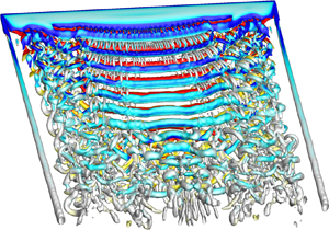
The difference in pressure between the upper and lower surfaces of the wing results in modification of the flow near the wing tip of a finite wing, causing the formation of a wing-tip vortex. This streamwise vortex interacts with the vortex shedding to further modify the flow. We compare the flow past a finite wing of  $sAR = 5$ with that past an EEW to understand the differences and their effect on aerodynamic coefficients at various $\alpha$. The $Q (=0.1)$ isosurface of instantaneous flow coloured with the spanwise component of vorticity ( $\omega _z = \pm 2$) for an $sAR = 5$ wing at various angles of attack is shown in figure 4. The wing-tip vortex suppresses the vortex shedding near the tip of the wing. In addition, it weakens the vortex shedding over the bulk of the span compared with that for the EEW. As a result, at $\alpha = 8^{\circ }$, the vortex shedding for the finite wing is quite weak compared with that of the EEW (see figures 3a and 4a).

Figure 4. Flow past the  $sAR = 5$ wing at $Re = 1000$: $Q (=0.1)$ isosurface for an instantaneous flow coloured with the spanwise component of vorticity ( $\omega _z = \pm 2$) for $\alpha =$ (a) $8^{\circ }$, (b) $10^{\circ }$, (c) $12^{\circ }$ and (d) $14^{\circ }$. The wing-tip vortex, central and end cells, dislocations, vortex splitting, vortex linkages and arch vortices are identified in the images. The inset in (d) shows the flow mirrored about the mid-span of the wing to visualize the arch vortices.
According to Helmholtz's theorem (Batchelor Reference Batchelor1967), a vortex must extend to the boundaries of the fluid or form a closed path. The spanwise vortices of an EEW extend to the lateral boundaries of the computational domain (see figure 3). However, owing to the wing-tip vortex, linkages form between vortices of opposite polarity near the tip of a finite wing. They are clearly seen in figure 4(b–d) for  $\alpha \ge 10^{\circ }$. Figure 5 shows the linkages via the $Q$ isosurface as well as a few vortex lines that pass through the core of an adjacent pair of counter-rotating vortices and connect to form a closed loop. We note that the linkages are not clear for $\alpha =8^{\circ }$ from the $Q$ isosurface (figure 4a). However, vortex lines in figure 5(a) clearly show the linkages even at this $\alpha$. Similar linkages have been reported for a finite wing (Zhang et al. Reference Zhang, Hayostek, Amitay, He, Theofilis and Taira2020) and flow past a circular cylinder near the side wall (Mittal et al. Reference Mittal, Pandi and Hore2021). Another flow feature observed at $\alpha = 14^{\circ }$ is the arch vortices in the mid-span region and at streamwise locations far downstream of the wing. These appear more clearly in images that show the flow for the full span of the wing. The inset in figure 4(d) shows a close-up view of the arch vortices for the full span. This image is constructed by mirroring the flow about the mid-span of the wing. A study to assess the effect of the symmetry boundary condition at the mid-span to constrain the flow is presented in Appendix C. The flow for the full span of the wing is computed for certain cases and compared with those for the half-span. It reveals that computations with half-span and full span lead to the same results. Arch vortices for $sAR = 1$ and $4$ are shown in the appendix. They are very similar to those reported in earlier studies for flow past a non-stationary wing (Visbal, Yilmaz & Rockwell Reference Visbal, Yilmaz and Rockwell2013; Rockwood et al. Reference Rockwood, Medina, Garmann and Visbal2019; Visbal & Garmann Reference Visbal and Garmann2019).

Figure 5. Flow past the  $sAR = 5$ wing at $Re = 1000$: $Q (=0.1)$ isosurface for an instantaneous flow coloured with the spanwise component of vorticity for $\alpha =$ (a) $8^{\circ }$ and (b) $10^{\circ }$. A few vortex lines that pass through the core of the adjacent pair of counter-rotating vortices connect to form a closed loop.
An interesting aspect of vortex shedding on a wing of finite span is the formation of cells. This has been studied in detail for bluff body flows (Gerrard Reference Gerrard1978; Eisenlohr & Eckelmann Reference Eisenlohr and Eckelmann1989; Williamson Reference Williamson1989; Behara & Mittal Reference Behara and Mittal2010; Mittal et al. Reference Mittal, Pandi and Hore2021). The variation of frequency of vortex shedding along the span is used to identify the number of cellular structures in the wake (Williamson Reference Williamson1989; Behara & Mittal Reference Behara and Mittal2010; Mittal et al. Reference Mittal, Pandi and Hore2021). The frequency of vortex shedding is constant within a cell. Similar to the flow of an EEW, the axis of the primary vortices shed from a wing of  $sAR = 5$ and $\alpha = 8^{\circ }$ is parallel to the span of the wing and the frequency of vortex shedding is the same at all spanwise locations, resulting in a single cell across the span. With an increase in angle of attack, the primary vortices are no longer parallel to the span of the wing. Furthermore, the vortex shedding occurs in two cells for $\alpha \ge 10^{\circ }$. We refer to the cell near the mid-span as the central cell and the one towards the wing tip as the end cell. The frequency of vortex shedding changes across the boundary of adjacent cells. A larger number of vortices, per unit time, are shed along one part of the span compared with other. Periodically in time, the extra vortex in the cell with a larger number of vortices connects with the neighbouring vortices in the adjacent cell leading to the formation of ‘knots’ (Eisenlohr & Eckelmann Reference Eisenlohr and Eckelmann1989) or ‘dislocations’ (Williamson Reference Williamson1989; Zhang et al. Reference Zhang, Hayostek, Amitay, He, Theofilis and Taira2020; Mittal et al. Reference Mittal, Pandi and Hore2021).
Dislocations can be of several kinds (Mittal et al. Reference Mittal, Pandi and Hore2021). For example, a pair of vortices of the same polarity in one cell may connect with a single vortex of the same polarity in an adjoining cell to form a fork-type ( $D_f$) dislocation. A modification to the fork-type dislocation was reported by Mittal et al. (Reference Mittal, Pandi and Hore2021) wherein vortices of opposite polarity form an additional linkage along with those in a fork-type dislocation. This is referred to as the connected fork-type dislocation. Another variant is the mixed-type dislocation that is of a fork type at one instant and a connected fork type at another instant (Mittal et al. Reference Mittal, Pandi and Hore2021). Vortex dislocations are marked in figure 4(b–d). Mixed-type dislocations are observed at $\alpha = 10^{\circ }$ while they are of fork type at $\alpha = 14^{\circ }$. The mixed-type dislocations have been observed earlier in bluff body flows. However, they are being reported for a finite wing for the first time. An interesting feature of the dislocations at $\alpha = 12^{\circ }$ is that the vortices split and reconnect in the far wake forming fork-type and reverse fork-type dislocations. As a result, a single cell in the near wake degenerates to two cells in the far wake. We note that this phenomenon has not been reported earlier in any flow.
4.2. Review of lifting line theory
We briefly review the lifting line theory for a finite wing and propose a small modification to apply it to relatively low  $Re$ flows. Consider a rectangular wing of span $b$ with no twist and the same airfoil section of chord length $c$ all along the span (see figure 1), placed in a uniform flow at an angle of attack, $\alpha$. We refer to $\alpha$ as the geometric angle of attack. The airfoil is assumed to be symmetric. The lifting characteristic of the wing is modelled by an infinite number of horseshoe vortices. The bound vortex of each horseshoe vortex lies along the quarter-chord line of the wing forming a ‘lifting line.’ The downwash induced by the vortices, estimated using the Biot–Savart law, results in tilting of the local lift vector at each spanwise station by $\alpha _i(z)$, referred to as the induced angle of attack. The effective angle of attack experienced by the local airfoil at each spanwise section is therefore $\alpha _{e}(z)=\alpha -\alpha _i(z)$. Assuming that the flow along the span is not significant, the local lift coefficient at each span location is estimated from the Kutta–Joukowski theorem as $C_l(z) = 2 \varGamma (z) / U c$, where $\varGamma (z)$ is the circulation at each spanwise section (Bertin Reference Bertin2002; Anderson Reference Anderson2017). Here $C_l(z)$ is also related to the effective angle of attack as $C_l(z) = \alpha _{e}(z)a_o$, where $a_o$ is the lift curve slope of the airfoil section. Equating the local lift coefficient obtained from these two approaches results in the following equation for circulation:
 \begin{equation} \alpha = \frac{{2 \varGamma(z)} }{{a_o U c}} + \frac{1 }{{4 {\rm \pi}U}} \int_{{-}b/2}^{b/2} \frac{{{\rm d}\varGamma}/{{\rm d}z} }{{z_o-z}} \,{\rm d}z. \end{equation}
 Using a transformation  $z = -b/2\cos \theta$, $0 \le \theta \le {\rm \pi}$, the spanwise variation of circulation is approximated using a Fourier sine series with $N$ coefficients: $\varGamma (\theta ) = 2 b U \sum _{1}^{N} {A_n~{\rm sin}~n\theta }$. Substitution of this approximation of $\varGamma$ in (4.1) and rearranging the terms results in the following equation that can be utilized to estimate the Fourier coefficients for $\varGamma (\theta )$:
 \begin{equation} \alpha = \frac{{2 b} }{{a_oc}} \sum _{1}^{N} {A_n\sin n\theta} + \sum_{1}^{N} nA_n\frac{\sin n\theta}{\sin\theta}. \end{equation}
 A collocation method is used to generate  $N$ equations at the same number of discrete spanwise locations. The collocation points are distributed all along the span. However, their density increases towards the wing tip. The resulting Fourier coefficients are utilized to estimate the spanwise distribution of the coefficient of lift ( $C_l(\theta ) = 4 b U c \sum _{1}^{N} {A_n\sin n\theta }$), the total lift coefficient for the finite wing ( $C_L = A_1 {\rm \pi}b c$) and the total induced drag coefficient (Bertin Reference Bertin2002; Anderson Reference Anderson2017):
 \begin{equation} C_{Di} = \frac{{C_L}^2 }{{{\rm \pi} AR}} \left(1 + \sum_{2}^{N} n \left(\frac{A_n}{A_1}\right)^2 \right). \end{equation}
In the classical lifting line theory, the slope of the variation of the local lift coefficient with angle of attack is assumed to be  $2{\rm \pi} \,{\rm rad}^{-1}$ for a thin airfoil (Bertin Reference Bertin2002; Anderson Reference Anderson2017). Unlike at large $Re$, the lift curve slope ( $a_o$) for the airfoil section at $Re = 1000$ is much lower. We estimate $a_o$ from direct numerical simulations at various $\alpha$ for an EEW, and utilize this estimated value in (4.1) and (4.2) to obtain the coefficients of a finite wing.
4.3. Force coefficients
Figure 6 shows the variation of time-averaged aerodynamic force coefficients and aerodynamic efficiency, with  $\alpha$, for an EEW and $sAR = 5$ wing at $Re = 1000$. As expected, the lift coefficient of a finite wing is lower than that for the EEW at each $\alpha$. It is inline with lifting line theory (Prandtl Reference Prandtl1921) wherein the finite wing, unlike an EEW, experiences a reduction in the effective angle of attack at each spanwise section. The prediction from the lifting line theory, with a small modification to account for the low $Re$ flow, is also shown in figure 6(a). Compared with flows at high $Re$ (Winkelmann et al. Reference Winkelmann, Barlow, Saini, Anderson and Jones1980; Sheldahl & Klimas Reference Sheldahl and Klimas1981), the lift curve slope at $Re = 1000$ is much lower. Consistent with the observations of Taira & Colonius (Reference Taira and Colonius2009) and Zhang et al. (Reference Zhang, Hayostek, Amitay, He, Theofilis and Taira2020), unlike at high $Re$, as indicated by the $C_L-\alpha$ curve, the flow does not exhibit stall at low $Re$. The drag coefficient shown in figure 6(b) from the lifting line theory is the sum of $\overline {C_D}$ for the EEW and the estimate of the induced drag coefficient for the finite wing. The induced drag is due to the tilting of the local lift vector. Also shown in the figure is the time-averaged drag coefficient from the computations for the viscous flow for the EEW as well as the $sAR=5$ finite wing. Contrary to the prediction from the lifting line theory, the present results show that the drag coefficient for the finite wing is lower than that for the EEW. Computations have also been carried out to obtain the steady flow by leaving out the unsteady terms in the governing equations. It is found that the drag coefficient for the EEW and $sAR=5$ wing are quite comparable; the values for the EEW are marginally higher. Furthermore, they are both lower than those for the time-averaged flow. The higher difference in the drag coefficient for the unsteady flow, between the finite wing and EEW, is primarily because of reduced vortex shedding activity in the finite wing owing to the wing-tip vortex. We investigate this further in a later section in the paper. The loss in lift for the finite wing outweighs the decrease in drag leading to its overall decrease in aerodynamic efficiency compared with the EEW, as shown in figure 6(c).

Figure 6. Flow past an EEW and  $sAR = 5$ wing at $Re = 1000$: variation of the time averaged (a) $\overline {C_L}$, (b) $\overline {C_D}$ and (c) $\overline {C_L}/\overline {C_D}$ with angle of attack. The data obtained using lifting line theory (LLT) (Prandtl Reference Prandtl1921) are plotted in each image. The best linear fit for the lift coefficient of an EEW is shown in (a) via the dashed green line.
Figure 7(a) shows the spanwise variation of the local lift coefficient for the time-averaged flow for different  $\alpha$. Also shown in the figure is the distribution from the lifting line theory (Prandtl Reference Prandtl1921). As per the lifting line theory, the local lift coefficient on a wing with a rectangular planform is maximum at the wing root and decreases monotonically towards the wing tip. The lift distribution from the computations at $Re=1000$ is in good agreement with that from the lifting line theory for $\alpha \le 8^{\circ }$. However, a non-monotonic variation is revealed for $\alpha \ge 10^{\circ }$. A local maximum is seen near the wing-tip region for $\alpha \ge 12^{\circ }$. A similar observation was made by Zhang et al. (Reference Zhang, Hayostek, Amitay, He, Theofilis and Taira2020) for flow at large $\alpha$ at $Re = 400$. We attribute the non-monotonic distribution of $\overline {C_l}$ to streamwise vortices that alter the distribution of circulation along the span. This is explained later in § 7 via a discrete vortex model. The spanwise variation of $\overline {C_d}$ is shown in figure 7(b). Also plotted is the prediction from the lifting line theory. It is obtained by adding the induced drag coefficient at each section from the tilting of the local lift vector to the drag coefficient for the EEW. The figure brings out the limitation of the lifting line theory in prediction of drag at low $Re$.
$Re$.

Figure 7. Flow past the  $sAR = 5$ wing at $Re = 1000$: spanwise variation of the time-averaged sectional force coefficient (a) $C_l$ and (b) $C_d$ at various $\alpha$. The sectional force coefficient distribution from the simulation is compared with theoretical data obtained using lifting line theory (LLT).
5. Effect of aspect ratio
5.1. Flow structures
We investigate the effect of  $sAR$ at two representative angles of attack: $\alpha = 8^{\circ }$ and $14^{\circ }$. Vortex shedding is quite weak at $\alpha =8^{\circ }$ for the EEW. The wing-tip vortex on a finite wing weakens it further by reducing the suction on the upper surface of the wing, thereby reducing the adverse pressure gradient. As a result, the flow for $sAR \le 4$ at $\alpha = 8^{\circ }$ is devoid of vortex shedding. Vortex shedding is quite strong at $\alpha =14^{\circ }$ and its interaction with the wing-tip vortex results in interesting flow features. To further understand the interplay between the vortex shedding and wing-tip vortex, we explore the strength and structure of the wing-tip vortex later in the paper. The $Q$ isosurface of instantaneous flow for various $sAR$ is presented in figure 8. Vortex shedding is suppressed in the region close to the wing tip; the flow achieves a steady state for $sAR \le 0.25$ (figure 8a) while shedding is observed away from the wing tip for larger $sAR$. Vortex shedding for $sAR=0.5$ occurs via hairpin vortex structures (figure 8b). These hairpin vortices are different than those that appear in the wake of the EEW as a result of the mode C instability (figure 3c). The hairpin vortices resulting from the mode C instability, also reported by Pandi & Mittal (Reference Pandi and Mittal2019), have a significantly smaller spanwise wavelength compared with those for an $sAR=0.5$ wing. Similar hairpins are seen for a finite wing, away from the wing tip, albeit for high $sAR$ (see inset of figure 8g). The interaction of the hairpin vortices with the wing-tip vortex for $sAR=0.5$ as it convects downstream results in undulations and the formation of linkages. The structure of the linkage is highlighted in the inset in figure 8(b) that shows a close-up view of the flow mirrored about the mid-span of the wing. The flow for $sAR = 0.5$ was also computed for the full span of the wing. It is found that the flow retains symmetry about the mid-span and is identical to the flow for the half-span. Vortex linkages for $sAR \ge 2$ have a very different structure compared with that for $sAR=0.5$. As shown in figures 5 and 8(d–g), they form between spanwise vortices of opposite polarity and do not link them with the wing-tip vortices. The linkages for $sAR=1$ have attributes that are common to a low and high $sAR$ wing. They are shown in the close-up view in figure 8(c) and marked via broken lines and form in the near wake to link spanwise vortices of opposite polarity. As in the case of $sAR = 0.5$, they form an additional linkage with the wing-tip vortex as they convect downstream. Arch vortices form in the far wake near the plane of symmetry for $sAR \ge 1$. Unlike a hairpin vortex whose limbs are aligned streamwise (Zhang et al. Reference Zhang, Hayostek, Amitay, He, Theofilis and Taira2020), the limbs of an arch vortex are in the cross-flow direction (Visbal et al. Reference Visbal, Yilmaz and Rockwell2013; Rockwood et al. Reference Rockwood, Medina, Garmann and Visbal2019; Visbal & Garmann Reference Visbal and Garmann2019). The wake consists of one cell for $sAR \le 2$. Two cells are observed for $sAR \ge 3$ with a fork-type dislocation (described later in the paper) at their boundary. The vortex dislocation forms at the same spanwise location, at different time instants, for $sAR = 3$. However, it is generated at different spanwise locations for $sAR \ge 4$.

Figure 8. Flow past a finite wing at  $\alpha =14^{\circ }$ and $Re = 1000$: $Q (=0.1)$ isosurface for an instantaneous flow coloured with the spanwise component of vorticity ( $\omega _z = \pm 2$) for $sAR =$ (a) $0.25$, (b) $0.5$, (c) $1$, (d) $2$, (e) $3$, ( f) $4$ and (g) $7.5$. Various flow features such as central and end cells, dislocations, hairpin vortices, vortex linkages and arch vortices are identified in the images. The insets in (b) that show hairpin vortex and linkage for $sAR=0.5$ are with the flow mirrored about the mid-span of the wing.
5.2. Force coefficients and comparison with lifting line theory
The variation of the time-averaged lift and drag coefficient with  $sAR$ is plotted in figures 9(a) and 9(b), respectively. For reference, the coefficients for the EEW along with the estimates from lifting line theory for the finite wing are also shown. We note that the lifting line theory cannot be expected to yield good predictions for low sAR wings owing to the intrinsic three dimensionality of the flow. The lift coefficient increases with an increase in $sAR$ and approaches the value for an EEW. The drag coefficient, predicted by the viscous computations, shows a very interesting trend with an increase in $sAR$. As per the lifting line theory, it decreases with an increase in $sAR$ due to a decrease in induced drag. However, the viscous computations for the finite wing reveal a non-monotonic variation of the time-averaged drag coefficient with an increase in $sAR$ (see figure 9b). It decreases with an increase in $sAR$ for $sAR \le 0.5$ and increases thereafter. Furthermore, for all $sAR$, it is smaller than that for the EEW. To explore this curious behaviour, we study the pressure and viscous contributions. It is found that the lift is primarily due to the pressure distribution and has very little contribution from viscous force (not shown here). The contributions from both the components is significant for drag and are shown in figure 9(c). Viscous force is the dominant contributor to drag for low $sAR (=0.25)$. Its contribution decreases while the pressure contribution increases with an increase in $sAR$. This explains the non-monotonic variation of $\overline {C_D}$ with $sAR$. The steady increase in the pressure contribution with $sAR$ causes the net drag coefficient to increase for $sAR > 0.5$, unlike the prediction from lifting line theory. We note that the wing-tip vortex reduces the suction on the upper surface near the wing tip. This leads to a reduced adverse pressure gradient and, thereby, reduced flow separation compared with an EEW. The fraction of wing span affected by the wing-tip vortex reduces with an increase in $sAR$, thereby causing a reduction in its effect. We explore the effect of a wing-tip vortex on vortex shedding. Figure 10(a) shows the spanwise variation of $\overline {v'v'}$ at ( $x/c=2.74$, $y/c=0.051$) for various $sAR$ along with that for an EEW. The Reynolds stress is significantly smaller near the wing tip for all $sAR$, indicating suppression of vortex shedding at those locations due to the wing-tip vortex. The net unsteadiness across the span, for each $sAR$, is estimated via spanwise integration of the Reynolds stress as ${\widetilde {v'v'}}=({\int _{0}^{b/2} \overline {v'v'}(z) \,{\rm d}z})/({\int _{0}^{b/2} \,{\rm d}z})$. Its variation with $sAR$ is shown in figure 10(b). We note that $\widetilde {v'v'}$ increases with an increase in $sAR$ and approaches the value for an EEW, signifying the increasing strength of vortex shedding with an increase in $sAR$. The trend is similar to the variation of drag coefficient with $sAR$ (figure 9b).

Figure 9. Flow past a finite wing at  $\alpha =14^{\circ }$ and $Re = 1000$: variation of the time averaged (a) $C_L$ and (b) $C_D$ with $sAR$ along with the prediction from lifting line theory for $C_L$ and $C_D$. Also shown in (c) is the variation of time averaged pressure ( $C_{Dp}$) and the viscous component ( $C_{Dv}$) of drag coefficient with $sAR$. The sectional $\overline{C_l}$ for steady and time-averaged flows is compared in (d).

Figure 10. Flow past a finite wing at  $\alpha = 14^{\circ }$ and $Re = 1000$: spanwise variation of (a) $\overline {v'v'}$ sampled at ( $x/c=2.74$, $y/c=0.051$) for various $sAR$. The net unsteadiness in the wake ( $\widetilde {v'v'}$), estimated via spanwise integration of $\overline {v'v'}$, is plotted in (b). Also shown in (a,b) is the data for the EEW.
The spanwise variation of sectional lift coefficient for the time-averaged flow for  $\alpha =14^{\circ }$ is shown in figure 9(d) for several $sAR$. As is observed for $sAR=5$ (see figure 7a), peak $\overline {C_l}$ is not at the root but close to wing tip for all $sAR$. The non-monotonic spanwise variation in $\overline {C_l}$ is due to the streamwise vortices that are formed near the wing-tip region. Images of the flow demonstrating the same are shown later in the paper. The peak $\overline {C_l}$ increases with an increase in $sAR$ for $sAR > 0.5$; $\overline {C_l}$ at the wing root also increases with an increase in $sAR$. Figure 9(d) shows the $\overline {C_l}$ distribution for the steady flow, computed by dropping the unsteady terms in the governing equations. We note that, compared with the steady flow, $\overline {C_l}$ is higher for the unsteady flow indicating that vortex shedding enhances $\overline {C_l}$. The higher unsteadiness for the EEW compared with the finite wing is also the reason for larger $\overline {C_D}$ for the former, as shown in figure 6(b). A further observation is that $\overline {C_l}$ for the steady flow at the wing root is quite similar for all the $sAR$ shown in the figure. Therefore, a larger increase of $\overline {C_l}$ for higher $sAR$ for the unsteady flow is indicative of a stronger vortex shedding. This is consistent with the observation from figure 8. Contrary to the prediction from lifting line theory, the peak $\overline {C_l}$ for the steady flow is also not at the wing root but at a location close to that for the unsteady flow. We will address this in a later section.
6. Cellular shedding and vortex dislocations
6.1. Frequency of vortex shedding
The number of cells in the wake can be identified from the frequency of vortex shedding measured at probes located at various locations along the span (Williamson Reference Williamson1989; Behara & Mittal Reference Behara and Mittal2010; Mittal et al. Reference Mittal, Pandi and Hore2021). The frequency is constant within a cell. The varying frequencies from multiple cells leave an imprint in the time histories of aerodynamic forces integrated along the span. The time histories of lift coefficient for various  $sAR$ along with their frequency spectra are presented in figure 11. For reference, the plots for the EEW are shown as well. The frequency is non-dimensionalized with the free-stream speed and a length scale corresponding to $d =c\sin \alpha$ (Hoarau et al. Reference Hoarau, Braza, Ventikos, Faghani and Tzabiras2003). The flow is steady for $sAR = 0.25$ and the associated lift coefficient is invariant with time (not shown in the figure). Single cell shedding for $sAR \le 2$ and two cell shedding is observed for $sAR \ge 3$ (see figure 8). The difference in the frequencies of central and end cells lead to low frequency modulation in the time histories (figure 11a). The Strouhal number for the two frequencies are referred to as $St_C$ and $St_E$, respectively, and are marked in figure 11(b). The frequency of vortex shedding has also been estimated from the time variation of the cross-flow component of velocity at various span locations in the near wake at ( $x/c=1.25, y/c=-0.068$). The frequencies so measured are identical to those marked in figure 11(b). The flow is explored in more detail later in the paper. The fluctuation in lift coefficient is largest for the EEW and decreases with a decrease in $sAR$.

Figure 11. Flow past a finite wing at  $\alpha =14^{\circ }$ and $Re = 1000$: (a) time histories of $C_L$ for the EEW and finite wing of various $sAR$, and (b) their frequency spectra. The Strouhal number corresponding to the dominant frequency for each spectrum is marked in the figure.
The variation of  $St_C$ and $St_E$ with $sAR$ is shown in figure 12(a). Here $St_C$ increases with an increase in $sAR$ and approaches the $St$ for the EEW. The vortex shedding frequency in the end cell is smaller than in the central cell. The difference in $St_C$ and $St_E$ is related to the beat frequency in the time signals of force coefficients and the probes lying at the boundary of the cells (Williamson Reference Williamson1989; Mittal et al. Reference Mittal, Pandi and Hore2021). It increases with an increase in $sAR$ up to $sAR=5$ beyond which it saturates to a constant value. Both $St_C$ and $St_E$ reach close to their respective saturated values at $sAR=5$. The variation of $St_C$ and $St_E$ with $\alpha$ is explored for the $sAR = 5$ wing; see figure 12(b). Also plotted is the $St$ for the EEW. Vortex shedding is very weak at $\alpha =8^{\circ }$ for the finite wing; the flow is close to steady near the wing tip (see figure 4a). Nevertheless, the Strouhal number is close to that for the EEW at this $\alpha$. The vortex shedding at $\alpha =10^{\circ }$ is relatively stronger and occurs in two cells (see figure 4b). The frequency of vortex shedding in the central cell, near the root, is close to that for the EEW; it is smaller in the end cell. A very interesting phenomenon is observed at $\alpha =12^{\circ }$. The near wake exhibits shedding in a single cell (figure 4c). However, vortex splitting downstream in the wake leads to two cells of vortex shedding in the far wake. Therefore, probes located in the near wake ( $x/c = 1.25, y/c = -0.068$) show a single cell with the same frequency of shedding along the span ( $St_C=0.159$), but indicate two cell shedding in the far wake ( $x/c = 11.62$, $y/c = -0.026$) ( $St_E=0.159, St_C=0.145$). We note that the $St$ shown in figure 12(b) for $\alpha = 12^{\circ }$ is in the near wake where the shedding is in a single cell. The central cell experiences a decrease in shedding frequency in the downstream wake. Unlike at other $\alpha$, $St_C$ is smaller than $St_E$. The frequency of occurrence of dislocation, the difference in $St_E$ and $St_C$, increases with an increase in $\alpha$.

Figure 12. Flow past a finite wing at  $Re = 1000$: variation of non-dimensional vortex shedding frequency in the central cell ( $St_C$) and end cell ( $St_E$) with (a) $sAR$ for $\alpha = 14^{\circ }$ and (b) $\alpha$ for $sAR = 5$. The $St$ for EEW is also marked. The frequency is estimated from probes placed along the span in the near wake at ( $x/c = 1.25$, $y/c = -0.068$).
The dislocations in two cell vortex shedding are of a varied kind depending on the combination of  $sAR$ and $\alpha$. They are of mixed type ( $D_{f-fc}$) (Mittal et al. Reference Mittal, Pandi and Hore2021), fork type ( $D_f$) (Williamson Reference Williamson1989; Mittal et al. Reference Mittal, Pandi and Hore2021) and a mix of fork ( $D_f$) and reverse fork type ( $D_{rf}$) reported for the first time in the present study. Figure 13 shows a summary of the various states of flow in the $sAR\unicode{x2013}\alpha$ plane. The classification is based on the type of dislocations and number of cells in the flow. The parameters for which the flow achieves a steady state is also shown. The boundaries of the various regimes are indicative extents where a similar flow structure is expected. The hatched region in the figure shows the regime for which the dislocation is generated at various spanwise locations. These features are described in detail in the following sections.

Figure 13. Flow past a finite wing: classification of the flow in the  $sAR\unicode{x2013}\alpha$ plane on the basis of the number of cells, type of dislocation and its formation along the span. The boundaries of the various regions are not exact, but indicative in nature and are based on the cases for which computations have been carried out and marked by hollow symbols. The cases for which a full-span simulation is initiated from the solution from half-span, by reflecting it about the mid-span, are highlighted using solid symbols. The dislocations, for two cell shedding, are generated at the same spanwise location except in the hatched zone where they are formed at different spanwise locations at different time instants. Here $D_f$, $D_{fc}$ and $D_{rf}$ indicate fork-type, connected fork-type and reverse fork-type dislocations.
6.2. Mixed-type dislocation ( $D_{f-fc}$) generated at the same spanwise location: $sAR = 5$, $\alpha = 10^{\circ }$


Dislocations occur at the boundary of cells with a different vortex shedding frequency. We present an example of flow wherein the dislocation is always generated at the same spanwise location. We estimate  $\widetilde {St}_v$ from each time period of the time history of the cross-flow component of velocity at various spanwise locations in the near wake ( $x/c = 1.25$, $y/c = -0.0068$). We note that $\widetilde {St}_v$ is the unsteady vortex shedding frequency estimated from each time period while that shown in figure 12 is from the fast Fourier transform of the entire time history of the unsteady signal. The spatio-temporal variation of $\widetilde {St}_v$ is presented in figure 14(a). Vortex dislocations can be identified from a spatial change in the local vortex shedding frequency, $\widetilde {St}_v$ (Mittal et al. Reference Mittal, Pandi and Hore2021). Behara & Mittal (Reference Behara and Mittal2010) further observed that the appearance of vortex dislocations coincides with local minima in $\widetilde {St}_v$ followed by its sharp rise. Three dislocations, $D_1$, $D_2$ and $D_3$, are marked in figure 14(a). They appear at $t = 175.23$, $196.23$ and $217.33$, respectively, at the same spanwise location. The time period of formation of the dislocations is ${\sim }21$ time units and corresponds to a frequency of $0.0476$. The frequency of appearance of dislocations can also be estimated from the beat frequency in the time signal near the junction of the cells (Williamson Reference Williamson1989; Mittal et al. Reference Mittal, Pandi and Hore2021). The beat frequency estimated from the time history of the cross-flow component of velocity is $0.0458$, and is in good agreement with the estimate from the variation of $\widetilde {St}_v$.

Figure 14. Flow past the  $sAR = 5$ wing at $\alpha =10^{\circ }$ and $Re = 1000$: (a) spatio-temporal variation of $\widetilde {St}_v$ obtained using a probe placed at $x/c = 1.25$ and $y/c = -0.068$. The $Q (=0.1)$ isosurface for an instantaneous flow coloured with the spanwise component of vorticity ( $\omega _z = \pm 2$) at two time instants is presented in (b,c). Fork-type ( $D_f$) and connected fork-type ( $D_{fc}$) dislocation is marked in (b,c). Results are shown for (b) $t = 178.386$, (c) $t = 180.886$.
Images of the isosurface of  $Q$ coloured with the spanwise component of vorticity are presented in figure 14(b,c) at two time instants. The dislocation is of a fork type at $t = 178.386$ (figure 14b). At $t = 180.886$ (figure 14c), a linkage between vortices of opposite polarity results in the formation of a ring-type vortex structure in addition to a fork-type dislocation. Mittal et al. (Reference Mittal, Pandi and Hore2021) referred to this as the mixed-type dislocation in their investigation of flow past a cylinder in the presence of a side wall. To the best of our knowledge, this type of dislocation is being reported for the first time in the wake of wings.
6.3. Fork-type ($D_f$) dislocation generated at varying spanwise locations: $sAR =5$, $\alpha = 14^{\circ }$


Dislocations are formed at varying spanwise locations for  $sAR \ge 4$ at $\alpha = 14^{\circ }$ (see figure 13). The spatio-temporal variation of $\widetilde {St}_v$ for $sAR = 5$ is shown in figure 15(a). Dislocations formed at various time instants are marked in the figure as $D_1-D_6$. Each occurrence is at a different spanwise location between $z/c=0.89$ to $1.9$. The time period between successive occurrence also varies. The average dislocation frequency is estimated to be $0.091$. It is in good agreement with the beat frequency ( $=0.092$) estimated from the time signal of the cross-flow component of velocity in the near wake. The instantaneous flow is shown in figure 15(b–e). The first two images show dislocation $D_1$ as it convects downstream, while the other two images show $D_3$. Both $D_1$ and $D_3$ are of a fork type ( $D_f$) and appear at different spanwise locations resulting in a time-varying span length of the end and central cells. However, once generated, each dislocation convects along the same spanwise location. Unlike in the present study, the dislocation at lower $Re (= 400)$ undergoes a spanwise movement as it convects (Zhang et al. Reference Zhang, Hayostek, Amitay, He, Theofilis and Taira2020).

Figure 15. Flow past the  $sAR = 5$ wing at $\alpha = 14^{\circ }$ and $Re = 1000$: (a) spatio-temporal variation of $\widetilde {St}_v$ obtained using a probe placed at $x/c = 1.25$ and $y/c = -0.068$. The $Q (=0.1)$ isosurface for an instantaneous flow coloured with the spanwise component of vorticity ( $\omega _z = \pm 2$) at various time instants is presented in (b–e). Also marked are the dislocation $D_1$ in (b–c) and $D_3$ in (d–e). Results are shown for (b) $t = 60.176$, (c) $t = 61.842$, (d) $t = 77.994$, (e) $t = 79.298$.
6.4. Fork ($D_f$) and reverse fork-type ($D_{rf}$) dislocations due to vortex splitting and reconnection: $sAR = 5$, $\alpha = 12^{\circ }$


Unlike for other flows,  $\alpha =12^{\circ }$ exhibits formation of dislocations in the far wake ( $x/c \sim 8$). The spatio-temporal variation of $\widetilde {St}_v$ for a probe in the near wake shows a single cell shedding while it shows the appearance of dislocations rather close to the wing root in the far wake. Figure 16(a) shows that the vortex shedding frequency at the wing root shows periodic variations with time while it is approximately constant with time, over the outer span. The instantaneous flow presented in figure 16(b) shows that the vortices are released from the wing at an oblique angle in the wake. They tend to align themselves parallel to the wing, especially near the wing root, as they convect downstream. In the process they undergo splitting and reconnection leading to a dislocation in the far wake. A reverse fork-type dislocation ( $D_{rf}$), on the far right, is marked in the image. The dislocation forms when two vortices of the same polarity in the end cell connect to a vortex of the same polarity in the adjoining cell. Some of the vortices marked in the near wake in this panel are identified in figure 16(c) at a later time as they convect downstream. While the dislocation seen in figure 16(b) is washed out of the frame at a later time, a new dislocation appears in figure 16(c) as a result of splitting and reconnection of vortices as shown. Also, a fork-type dislocation ( $D_{f}$) forms in the later part of the wake. The convection of the vortices and the dislocations lead to the state shown in figure 16(d). Dislocation $D_{f}$ is washed out, while $D_{rf}$ moves in the far wake.

Figure 16. Flow past the  $sAR = 5$ wing at $\alpha = 12^{\circ }$ and $Re = 1000$: (a) spatio-temporal variation of $\widetilde {St}_v$ obtained using a probe placed at $x/c = 1.25$ and $y/c = -0.068$. The $Q (=0.05)$ isosurface for an instantaneous flow coloured with the spanwise component of vorticity ( $\omega _z = \pm 1$) at various time instants is presented in (b–d). The vortex splitting and reconnections are illustrated using coloured solid lines. The filled black circles show the inter-connection between the vortices. Here $D_f$ and $D_{rf}$ refer to fork-type and reverse fork-type dislocations, respectively. Results are shown for (b) $t = 189.61$, (c) $t = 192.61$,(d) $t = 200.61$.
6.5. Role of cellular shedding in spanwise variation of r.m.s. of aerodynamic coefficients
We explore the effect of cellular shedding observed for  $sAR \ge 3$ (see figure 8) on the unsteadiness of flow via spanwise variation of the r.m.s. of the lift and drag coefficient and $\overline {u'v'}$ component of Reynolds stress in the near wake. The same is shown in figure 17 along with the flow for $sAR=2$ and $4$ associated with a single cell and two cells, respectively. The r.m.s. coefficients and $\overline {u'v'}$ are maximum close to the wing root for $sAR=2$. However, the unsteadiness in the flow is closer to the wing tip than the wing root for $sAR=4$. For example, $C_{l_{rms}}$ achieves a maxima at $z/c\sim 2.6$. We note the nearly parallel shedding for $sAR=2$ and varying oblique angle of the vortices in the near wake for $sAR=4$. The spanwise minima in the unsteadiness for $sAR=4$ occurs at the location where the oblique angle of the shed vortices is maximum. The unsteadiness near the wing tip is very weak for both $sAR$.

Figure 17. Flow past a  $\alpha = 14^{\circ }$ wing at $Re = 1000$: (a,b) spanwise variation of sectional r.m.s. of lift and drag coefficient, (c,d) $Q (=0.1)$ isosurface for an instantaneous flow coloured with the spanwise component of vorticity ( $\omega _z = \pm 2$) and (e, f) $\overline {u'v'}$ component of Reynolds stress on the $y\unicode{x2013}z$ plane at $x/c = 3.5$. The quantities are for $sAR = 2$ (left) and $sAR = 4$ (right).
7. Streamwise vortices
Figures 7 and 9(d), that show the spanwise variation of sectional aerodynamic coefficients, reveal a significant departure of the present results from the predictions of lifting line theory. We attribute the difference to the presence of other streamwise vortices in addition to the wing-tip vortices. Figure 18(a,b) shows the instantaneous flow at  $\alpha = 12^{\circ }$ and $14^{\circ }$ for the $sAR = 5$ wing. Superimposed on these images is the $Q$ isosurface for the time-averaged flow at respective $\alpha$. Both flows show strong wing-tip vortices. The time-averaged flow reveals additional streamwise vortices. The prominent ones are a result of the vortex linkages as they convect downstream in the wake. Figure 19 shows the $Q$ isosurface for a time-averaged flow for various $sAR$ at $\alpha = 14^{\circ }$. The streamwise vortices are stronger near the wing-tip region and weaker towards the wing root.

Figure 18. Flow past the  $sAR = 5$ wing at $Re = 1000$: $Q (= 0.1)$ isosurface for an instantaneous flow coloured with the streamwise component of vorticity ( $\omega _x = \pm 1$, blue-white-red) for $\alpha =$ (a) $12^{\circ }$ and (b) $14^{\circ }$. Also superimposed is the $Q$ iso-surface for time-averaged flow coloured with streamwise component of vorticity ( $\omega _x = \pm 1$, cyan-white-yellow) in each figure.

Figure 19. Flow past a finite wing at  $\alpha = 14^{\circ }$ and $Re = 1000$: $Q (=0.01)$ isosurface for a time-averaged flow coloured with the streamwise component of vorticity ( $\omega _x = \pm 2$) for $sAR =$ (a) $0.5$, (b) $1$, (c) $3$ and (d) $5$.
$5$.
7.1. Do streamwise vortices exist in a steady flow?
Figure 9(d) shows that, unlike the prediction from lifting line theory presented in figure 7(a), the sectional lift coefficient for the steady flow also shows a peak closer to the wing tip and not at the wing root. A natural question that arises is: ‘Is the steady flow also associated with streamwise vortices other than wing-tip vortices?’ The  $Q$ isosurface, coloured with the streamwise component of vorticity, is shown in figure 20 for the steady flow for the $sAR=5$ wing at various $\alpha$. The flow is obtained by dropping the unsteady terms from the flow equations. The time-averaged and steady flows are very similar for $\alpha \le 8^{\circ }$ (not shown here) as the vortex shedding is relatively weak; the wing-tip vortices are the only prominent streamwise vortices. Additional streamwise vortices appear near the wing tip at larger $\alpha$. As seen from figure 20, they increase in number, originate from a larger length of the span and become stronger with an increase in $\alpha$. At $\alpha =14^{\circ }$ they virtually occupy the entire span (figure 20c). Interestingly, for a wing with larger $sAR$ (for example, $sAR=7.5$, shown in figure 20d), the spanwise extent of the generation of streamwise vortices is similar to that for $sAR=5$ (figure 20c).

Figure 20. Flow past the  $sAR = 5$ wing at $Re = 1000$: $Q (=0.01)$ isosurface for a steady flow coloured with the streamwise component of vorticity ( $\omega _x = \pm 2$) for $\alpha =$ (a) $10^{\circ }$, (b) $12^{\circ }$, (c) $14^{\circ }$. Also presented in (d) is the flow of the $sAR = 7.5$ wing at $\alpha = 14^{\circ }$.
7.2. Effect of streamwise vortices on spanwise lift distribution
We attempt to explain the local maximum observed in the spanwise distribution of the sectional lift coefficient by using a discrete model of the streamwise vortices. Figure 21(a,b) shows the cores of streamwise vortices corresponding to the steady and time-averaged flows for  $\alpha = 14^{\circ }$ and the $sAR = 5$ wing. Also shown in this schematic is the bound vortex on the wing. The circulation of each streamwise vortex is estimated by carrying out line integration of the velocity field along a closed curve, enclosing the vortex, in the $y\unicode{x2013}z$ plane at $x/c=3.5$. To enable a good estimate, the closed curve is chosen to be as large as possible while ensuring that it does not include adjacent vortices. The circulation is non-dimensionalized using the free-stream speed and chord of the airfoil. The streamwise component of vorticity in the $y\unicode{x2013}z$ plane at $x/c = 3.5$ is presented in figure 21(d,e) for the steady and time-averaged flows, respectively. A streamwise vortex with a component of its vorticity pointing in the positive $x$ direction is considered positive and is marked in red in the schematics shown in figure 21(a,b). The circulation of each vortex ‘ $i$’ is denoted by $\varGamma _i$ with the index increasing from the wing tip towards the mid-span. The indices for all the major streamwise vortices are marked in figure 21(a–e) and their respective $\varGamma _i$ plotted in figure 21(f, g); $\varGamma _1$, for example, denotes the strength of the wing-tip vortex. Also shown in figure 21(f, g) is the circulation, $\varGamma _z$, along the bound vortex. It is estimated at various spanwise locations via line integration of the velocity field on a closed curve in the $x\unicode{x2013}y$ plane that encloses the airfoil section. We utilize a circle whose centre is located at the mid-chord of the airfoil. The value of $\varGamma _z$ estimated on various circular curves with radius $0.51c-1c$ is very close. The sign convention is indicated in figure 21(c). We recall that $\varGamma _z$ is related to the sectional lift coefficient via the Kutta–Joukowski theorem for 2-D flows (Bertin Reference Bertin2002; Anderson Reference Anderson2017). A reasonable match is seen between $\varGamma _z$ and $C_l/2$ for both the time-averaged and steady flows except in the region of the wing tip, where, expectedly, the flow is highly three dimensional.

Figure 21. Flow past the  $sAR = 5$ wing at $\alpha = 14^{\circ }$ and $Re = 1000$: schematic showing the bound vortex and core of streamwise vortices including the wing-tip vortex for a (a) steady and (b) time-averaged flow. The wing surface is shown in a grey colour and the bound vortex in a solid black line. The sign convention for the circulation around the bound vortex is also shown in (c). Streamwise component of vorticity on the $y\unicode{x2013}z$ plane at $x/c = 3.5$ is shown for asteady flow in (d) and a time-averaged flow in (e). Shown in ( f,g) is the spanwise variation of circulation ( $\varGamma _z$) in the $x\unicode{x2013}y$ plane enclosing the airfoil section along with the sectional lift coefficient ( $C_l$) for the steady and time-averaged flows, respectively. Also shown in the same plot is the circulation of streamwise vortices $\varGamma _i$ and the strength of the bound vortex ( $\varGamma _b$).
Using the discrete vortex model, as shown in figure 21(a,b), we estimate the strength of the bound vortex at a spanwise location  $z_i$ by the expression $\varGamma _b(z_i) = \sum _{j=1}^{i}(-\varGamma _j)$. The same is shown in figure 21( f,g). For both, steady and time-averaged flows, $\varGamma _b(z_i)$ shows qualitatively the same behaviour as $\varGamma _z$ and $C_l/2$ confirming that the local peak in the spanwise variation of the sectional lift coefficient is due to streamwise vortices. Figure 21(a,b) shows that the streamwise vortices that are fairly evenly spread over the span of the wing in a steady flow relocate away from the root of the wing for the time-averaged flow, leading to an increased interaction and vortex strength. In general, the strength of vortices in the time-averaged flow is larger than in the steady flow. For example, $\varGamma _1$ and $\varGamma _2$ for the time-averaged flow are larger compared with the steady flow, even though their locations are quite comparable.
8. Wing-tip vortex
8.1. Strength of wing-tip vortex
We explore the dependence of the strength of the wing-tip vortex with angle of attack and aspect ratio of the wing. The circulation is estimated by carrying out integration along a closed curve lying in the  $y\unicode{x2013}z$ plane at $x/c=3.5$. The effect of the spatial extent of the curve on $\varGamma$ is assessed for the time-averaged flow at $\alpha =14^{\circ }$ and presented in Appendix D. Isovorticity curves ( $\overline {\omega _x}=C$) are utilized to carry out the integration. It is found that a curve corresponding to a value of $|C| \le 0.1$ provides a good estimate of $\varGamma$. The same has been utilized in this study. Figure 22(a) shows the variation of circulation, corresponding to the steady and time-averaged flows for the $sAR=5$ wing, with angle of attack. Here $\varGamma$ increases with an increase in $\alpha$. The variation is linear for the steady flow. However, the slope of the curve changes at $\alpha =8^{\circ }$; it is larger for the variations beyond $\alpha =8^{\circ }$. We recall that the streamwise vortices, other than the wing-tip vortices, become prominent beyond $\alpha =8^{\circ }$ (see figure 20). We attribute this change in slope of $\varGamma -\alpha$ variation to the appearance of additional streamwise vortices across the wing span. For the time-averaged flow, the linear variation up to $\alpha =8^{\circ }$ is followed by a nonlinear increase of $\varGamma$ with $\alpha$. In this regime the strength of the wing-tip vortex for the time-averaged flow is higher than that of the steady flow. This is also seen from figure 21( f,g) for $\alpha =14^{\circ }$. The effect of the aspect ratio of the wing on the strength of the wing-tip vortex is presented in figure 22(b) for $\alpha = 8^{\circ }$ and $14^{\circ }$. For $\alpha =8^{\circ }$, the vortex strength increases with an increase in $sAR$ up to $sAR=2$ and does not show any significant change beyond it. The variation in $\varGamma$ is more significant at $\alpha =14^{\circ }$. It increases with $sAR$ up to $sAR=5$ and does not show any appreciable increase beyond it. For each $sAR$, the strength of the wing-tip vortex for the time-averaged flow is larger than that for the steady flow.

Figure 22. Flow past a wing at  $Re = 1000$: variation of strength of the wing-tip vortex, $\varGamma$, with (a) $\alpha$ for $sAR = 5$ and (b) $sAR$ for $\alpha = 8^{\circ }$ and $14^{\circ }$. Here $\varGamma$ is non-dimensionalized using a free-stream speed and chord of the airfoil.
8.2. Model of wing-tip vortex
We utilize two models to estimate the radius of the wing-tip vortex: Rankine vortex (Rankine Reference Rankine1877) and Lamb–Oseen vortex (Saffman Reference Saffman1995; Jacquin et al. Reference Jacquin, Fabre, Sipp and Coustols2005). The core of a Rankine vortex is modelled by a forced vortex of strength  $\varGamma$ and radius $R$ while the outer zone is approximated by a free vortex. The Lamb–Oseen vortex is an exact solution of the Navier–Stokes equation. The velocity across the vortex decreases exponentially beyond its core of radius $R$. The tangential velocity distributions for the Rankine and Lamb–Oseen vortex are, respectively,
 \begin{gather} V_{\theta_{fo}} = \frac{\varGamma r}{2{\rm \pi} R^2}; V_{\theta_{fr}} = \frac{\varGamma}{2 {\rm \pi}r}; \end{gather}
 \begin{gather} V_{\theta_{LO}} = \frac{\varGamma}{2{\rm \pi} r}(1-e^{{-}r^2/R^2}). \end{gather}
A schematic of the two models is shown in figure 23(a). The models are applied to the time-averaged flow past the  $sAR = 5$ wing at $\alpha = 14^{\circ }$. Figure 23(b,c) shows the velocity distribution in the $y\unicode{x2013}z$ plane along lines parallel to the $y$ and $z$ axes and passing through the core of the wing-tip vortex at two streamwise locations $x/c = 3.5$ and $10$, respectively. Also shown in the figures, with broken lines, is the velocity distribution from the models given by (8.1) and (8.2). The value of $\varGamma$ is estimated from the computations (see figure 22). The value of $R$ is estimated from each of the two models as shown in figure 23(b,c) for the best approximation to the velocity profiles from direct time integration. Here $R$ is estimated using this procedure for various streamwise locations. The streamwise variation of $R$ alongside the best fit is shown in figure 23(d). We note that both the models yield virtually the same value of $R$. It increases linearly with an increase in $x/c$. A similar variation is also seen for the steady flow (not shown here). It is found that $R$ is larger for the time-averaged flow compared with the steady flow. Figure 24(a,b) shows the variation of $R$, at $x/c = 3.5$, with $\alpha$ and $sAR$, respectively. Here $R$ increases with an increase in the angle of attack. For a fixed $\alpha$, $R$ increases with an increase in $sAR$ up to $sAR=2$, beyond which it does not change with any further increase in $sAR$.

Figure 23. Flow past a finite wing for  $Re = 1000$: schematic of the Rankine (forced-free) vortex and Lamb–Oseen vortex model where $R$,
$R$,  $\varGamma$, $o'$,
$o'$,  $V_{\theta _{fo}}$, $V_{\theta _{fr}}$ and $V_{\theta _{LO}}$ represents the radius of the vortex, strength of the wing-tip vortex, core of the vortex, velocity for the Rankine (forced-free) vortex and Lamb–Oseen vortex, respectively. The variation of velocity distribution across the wing-tip vortex for a time-averaged flow of an $sAR = 5$ wing at $\alpha = 14^{\circ }$ is shown in (b) $x/c = 3.5$ and (c) $x/c = 10$. Also shown in broken lines are the curve obtained using the theoretical expressions. The variation of $R/c$, obtained using the Rankine and Lamb–Oseen vortex, with $x/c$ along with best linear fit is presented in (d).

Figure 24. Flow past a wing at  $Re = 1000$: variation of $R/c$ estimated at $x/c = 3.5$ with (a) $\alpha$ for an $sAR = 5$ wing and (b) $sAR$ at $\alpha = 8^{\circ }$ and $14^{\circ }$.
9. Conclusions
An incompressible flow past a rectangular wing with a NACA 0012 airfoil section for  $Re=1000$ has been investigated via a stabilized finite element method. Computations for an EEW for various angles of attack reveal transition of the wake. While the flow is steady at low angles of attack, vortex shedding commences at $\alpha \sim 8^{\circ }$. The flow becomes three dimensional for $\alpha$ beyond $12^{\circ }$ via the mode C instability that evolves to hairpin vortex structures. Simulations for a finite wing have been carried out for one half of the wing. The semi-aspect ratio and angle of attack considered in the study is $0.25 \le sAR \le 7.5$ and $0^{\circ } \le \alpha \le 14^{\circ }$. The suitability of symmetry conditions at the mid-span has been demonstrated via computations for the wing of the full span.
A finite wing is associated with wing-tip vortices that interact with vortex shedding leading to rich structures. The strength of the wing-tip vortex increases with an increase in  $\alpha$. At each $\alpha$, it increases with an increase in $sAR$ up to a certain aspect ratio, beyond which it achieves an almost constant value. Flow past an EEW has been compared with that on a finite wing for various $sAR$ and $\alpha$. Vortex shedding is suppressed along the entire span of the wing at $\alpha = 8^{\circ }$ for $sAR \le 4$. Weak vortex shedding is observed away from the wing tip while it continues to be suppressed near it for $sAR = 5$. The range of sAR for which the flow is steady is smaller at larger angles of attack. At $\alpha = 14^{\circ }$, the flow is steady for $sAR \le 0.25$. Hairpin vortices are shed at the mid-span for sAR = 0.5. They interact with the wing-tip vortices from the starboard and port sides of the wing, as they convect downstream, creating undulations and form linkages between them. The strength of vortex shedding in the mid-span region increases with an increase in $sAR$. However, the region near the wing tips continues to be devoid of shedding. As a result, the spanwise vortices of opposite polarity join to form linkages in the outboard region. The linkages for the $sAR = 0.5$ and $sAR \ge 2$ are qualitatively different. A mix of the two types of linkages is observed for $sAR = 1$. The interactions also result in the formation of arch vortices in the mid-span region for $sAR \ge 1$. The hairpin vortex structures, associated with mode C instability in the EEW (Pandi & Mittal Reference Pandi and Mittal2019), are not observed for low $sAR$. However, they appear in the central cell for higher $sAR$. It is to be noted that the hairpin vortices associated with $sAR = 0.5$ are different than those at higher $sAR$. The former are not due to the mode C instability and have a significantly larger spanwise wavelength.
Unlike for an EEW, where the axes of shed vortices are parallel to the wing and frequency of shedding is constant across the span, vortex shedding on a finite wing is oblique and cellular. For example, two cells form along the span of the wing for  $sAR \ge 3$ at $\alpha = 14^{\circ }$. The vortex shedding frequency in the central cell, that lies in the mid-span region, approaches that for the EEW. It is lower in the end cell that spans the outboard region of the wing. A dislocation demarcates the cells, with differing vortex shedding frequency. Various types of dislocations are observed for different combinations of $\alpha$ and $sAR$. These are the classical fork-type (Williamson Reference Williamson1989), connected fork-type (Mittal et al. Reference Mittal, Pandi and Hore2021) and the mixed-type (Mittal et al. Reference Mittal, Pandi and Hore2021) dislocations. In certain cases, the dislocations are generated at the same spanwise location at different times, while in others the dislocations appear at different spanwise locations with respect to time. However, in all cases, their convection is primarily streamwise with almost no spanwise movement. An additional type of dislocation, that is being reported for the first time, has been observed for $\alpha = 12^{\circ }$ for the $sAR=5$ wing. It is a consequence of splitting and reconnection of vortices as they convect away from the wing. The vortex shedding frequency in the very near wake is constant along the span. However, two cells are observed in the moderate to far wake downstream of the reconnection of vortices. These dislocations form fork-type and reverse fork-type connections in the vortices between the central and end cells.
The results from the computations are compared with the predictions from the lifting line theory. Unlike in the classical lifting line theory, where the lift curve slope for an airfoil is estimated for an inviscid flow, it is estimated from computations for the EEW at  $Re=1000$ in the present work. A surprising finding, for low $Re$, is that the drag coefficient for the finite wing is lower than that for the EEW. This is contrary to the prediction from the lifting line theory, according to which the drag coefficient for the finite wing should be higher owing to the induced drag. The present analysis reveals that the spillage of the flow at the wing tip reduces the peak suction on the upper surface, thereby resulting in a lower adverse pressure gradient. This leads to weaker vortex shedding and a lower pressure drag for the finite wing, compared with the EEW. The increase in unsteadiness in the flow is quantified by the increase in $\widetilde {v'v'}$ in the wake integrated over the span. Furthermore, since the effect of spillage reduces with an increase in aspect ratio of the wing, the drag coefficient increases with an increase in $sAR$ for $sAR>0.5$, unlike the prediction from lifting line theory. As expected, the force coefficients for the finite wing approach the values for an EEW with an increase in $sAR$.
The spanwise variation of the time-averaged sectional lift coefficient for  $\alpha \ge 10^{\circ }$ is found to be non-monotonic. Unlike the prediction from lifting line theory that predicts a maxima at the wing root, its maximum value is near the wing-tip region. Analysis of the flow reveals streamwise vortices in addition to the wing-tip vortex. They are observed in the steady flow as well. The wing-tip vortices are stronger for the unsteady flow as compared with the steady flow. The increase in their strength, with an increase in $\alpha$, is linear for the steady flow and nonlinear for the unsteady flow. The number and strength of vortices increases with an increase in the angle of attack. A discrete vortex model is utilized to relate the strength of the streamwise vortices to the spanwise variation of sectional lift coefficient. It is concluded that the non-monotonic spanwise variation of lift coefficient is caused by the streamwise vortex structures. It would be interesting to follow their evolution with an increase in $Re$ in a future study. The Rankine (forced-free) and Lamb–Oseen vortex model has been proposed for the wing-tip vortex. The radius of the vortex increases linearly with streamwise location. At a fixed streamwise location the radius is fairly constant for $sAR \ge 2$.
The fluctuating component of the sectional force coefficients also show an interesting variation along the span. They are maximum near the wing root for  $sAR \le 2$ when there is only one cell of vortex shedding and the vortices are shed parallel to the wing axis. However, their maxima is achieved at an outboard location on the wing for $sAR \ge 3$ that are associated with two cells of shedding and the oblique angle of the shed vortices, with respect to the wing axis, varies with time and along the span. The load distribution on the wing has an implication on the design of its structure and, therefore, its weight.
Acknowledgements
All the computations were performed using the high performance computational (HPC) facility at Indian Institute of Technology Kanpur (IITK), established with the assistance of Department of Science and Technology (DST), India. We also acknowledge the help from Mr Yuvraj in computation of some of the preliminary results and the lively discussions.
Declaration of interests
The authors report no conflict of interest.
Appendix A. Mesh convergence
A.1. Mesh in two dimensions
The spatial convergence of the finite element mesh in two dimensions is investigated at  $\alpha = 14^{\circ }$ and $Re = 1000$. Table 1 lists the three finite element meshes considered. The number of points on the surface of the airfoil are $200$, $250$ and $300$ for meshes $M_{2D}^1$, $M_{2D}^2$ and $M_{2D}^3$, respectively. The time integration of governing flow equations are carried out using a time step size $\Delta t = 0.002$. The time-averaged force coefficients along with their fluctuations obtained using three meshes are in good agreement. The difference in the lift and drag coefficients for meshes $M_{2D}^1$ and $M_{2D}^2$ is $1.7\,\%$ and $0.8\,\%$, respectively. The corresponding values for meshes $M_{2D}^2$ and $M_{2D}^3$ are $0.35\,\%$ and $0.65\,\%$, respectively. As the difference between meshes $M_{2D}^2$ and $M_{2D}^3$ is relatively low, we proceed with $M_{2D}^2$. To study the effect of time step size, computations are carried out on mesh $M_{2D}^2$ using $\Delta t = 0.001$. The difference in the lift and drag coefficients for $\Delta t = 0.002$ and $0.001$ is $0.14\,\%$ and $0.04\,\%$, respectively. This shows that mesh $M_{2D}^2$ and $\Delta t = 0.002$ provides adequate spatial and temporal resolution for $Re = 1000$. The results computed on mesh $M_{2D}^2$ are compared with the data from past studies for a NACA 0012 airfoil at $Re=1000$ for various $\alpha$. Figure 25(a,b) shows the variation of time-averaged lift and drag coefficients with angle of attack along with the data from earlier studies (Mittal & Tezduyar Reference Mittal and Tezduyar1994; Liu et al. Reference Liu, Li, Zhang, Wang and Liu2012; Kurtulus Reference Kurtulus2015; Meena et al. Reference Meena, Taira and Asai2017; Di Ilio et al. Reference Di Ilio, Chiappini, Ubertini, Bella and Succi2018). Very good agreement is observed between the results from various studies.
Table 1. Flow past a NACA 0012 airfoil at  $\alpha = 14^{\circ }$ and $Re = 1000$ in two dimensions: details of the finite element mesh along with the computed time-averaged coefficients and fluctuations.


Figure 25. Flow past a NACA 0012 airfoil at  $Re=1000$: comparison of time-averaged (a) lift and (b) drag coefficients with the data from earlier studies (Mittal & Tezduyar Reference Mittal and Tezduyar1994; Liu et al. Reference Liu, Li, Zhang, Wang and Liu2012; Kurtulus Reference Kurtulus2015; Meena et al. Reference Meena, Taira and Asai2017; Di Ilio et al. Reference Di Ilio, Chiappini, Ubertini, Bella and Succi2018). The data reported in the present study is obtained using mesh $M_{2D}^2$.
A.2. Mesh in three dimensions
A.2.1. End-to-end wing
Copies of mesh  $M_{2D}^2$ are stacked uniformly along the span to generate a mesh in three dimensions for the EEW. The span of the wing is $L_z=5 c$. Computations are carried out at $\alpha = 14^{\circ }$ and $Re = 1000$. Two meshes are considered: mesh $M_{3D}^1$ with $N_z=160$ and $M_{3D}^2$ with $320$ copies along the span. The details of the meshes as well as the results from the computations are listed in table 2. Also shown in the table is the spanwise wavelength of the three-dimensional vortex structures. The results from both the meshes are in very good agreement reflecting the adequacy of mesh $M_{3D}^1$ that is associated with an element size of $\Delta z \sim 0.031c$ along the span.
Table 2. Flow past an EEW of span  $L_z = 5c$ at $\alpha = 14^{\circ }$ and $Re = 1000$: details of the finite element meshes along with the computed time-averaged coefficients and fluctuations. Also listed is the spanwise wavelength of the three-dimensional flow structures. Here $N_z$ is the number of copies of mesh $M_{2D}^2$ stacked uniformly along the span.

A.2.2. Finite wing: $sAR = 5$

The mesh convergence study is extended to a finite wing with  $sAR = 5$ at $\alpha = 14^{\circ }$ and $Re = 1000$. The finite element mesh for a finite wing is generated by stacking mesh $M_{2D}^2$ on the wing and another mesh, $M_{2Dout}^2$, outside the span of the wing. Here $M_{2Dout}^2$ is identical to $M_{2D}^2$ outside the airfoil section, but contains additional grid points inside. It consists of $45\,760$ nodes and $91\,421$ elements. Unlike for the EEW, the 2-D mesh for the finite wing is stacked non-uniformly along the span. The element size $\Delta z$ is approximately $0.031c$ at the wing root and $0.0035 c$ near the wing tip. Three meshes with $N_z$ copies of the 2-D meshes, out of which $N_{wing}$ lie on the wing, are utilized for the convergence study. The details of the meshes along with the results obtained with them are listed in table 3. The difference in lift and drag coefficients for meshes $M_{3D}^3$ and $M_{3D}^4$ is $0.47\,\%$ and $0.27\,\%$, respectively. The corresponding values for the difference between values for meshes $M_{3D}^4$ and $M_{3D}^5$ are $0.34\,\%$ and $0.23\,\%$, respectively. The results from all the three meshes are in very good agreement. This is further highlighted in figure 26, which shows the chordwise variation of time-averaged coefficients for surface pressure and skin friction on the wing at a span location corresponding to $z/c = 1.75$. All the simulations in the present study for the finite wing with $sAR=5$ are carried out with mesh $M_{3D}^4$. The mesh for other $sAR$ is obtained by maintaining a similar spanwise resolution.
Table 3. Flow past the  $sAR = 5$ wing at $\alpha = 14^{\circ }$ and $Re = 1000$: time-averaged aerodynamic coefficients and their fluctuations obtained using three finite element meshes. Here $N_z$ denotes the number of copies of a 2-D mesh stacked along the lateral extent of the computational domain. Of these, $N_{wing}$ is the number of sections that lie on the wing.


Figure 26. Flow past the  $sAR = 5$ wing at $\alpha = 14^{\circ }$ and $Re = 1000$: chordwise distribution of time-averaged (a) $C_p$ and (b) $C_f$ distribution on the wing surface at $z/c = 1.75$ obtained using three different finite element meshes.
A.2.3. Finite wing: $sAR = 1.25$

The effect of the mesh is investigated for a finite wing with  $sAR = 1.25$ at $\alpha =5^{\circ }$ and $Re = 1000$. The lateral boundary of $sAR=1.25$ is located at a distance of $L_z=3c$ from the tip of the wing, while it is $10c$ for the $sAR=5$ wing (see figure 1). The procedure to generate the mesh is similar to that of $sAR = 5$ but with fewer copies of the 2-D meshes $M_{2D}^2$ and $M_{2Dout}^2$ along the spanwise dimension. Two meshes are considered. These meshes have the same 2-D mesh and differ in the number of 2-D sections stacked along the span. The details of the two meshes along with the results obtained from computations utilizing them are listed in table 4. The computations yield a steady flow. The results obtained from the two meshes are virtually identical. The lift and drag coefficients from the present study are in excellent agreement with those reported by Edstrand et al. (Reference Edstrand, Sun, Schmid, Taira and Cattafesta2018) ( $C_L=0.158$, $C_D=0.125$), confirming the adequacy of the present methodology and mesh to resolve the flow satisfactorily.
Table 4. Flow past the  $sAR = 1.25$ wing at $\alpha = 5^{\circ }$ and $Re = 1000$: aerodynamic coefficients obtained using two finite element meshes. Here $N_z$ denotes the number of copies of a 2-D mesh stacked along the lateral extent of the computational domain. Of these, $N_{wing}$ is the number of sections that lie on the wing.

Appendix B. Vortex identification criteria
Several methods have been proposed in the past to identify vortex cores in a flow. Some of the popular methods are the  $Q$,
$Q$,  $\lambda _2$ and $\varOmega$ criterion proposed by Hunt et al. (Reference Hunt, Wray and Moin1988), Jeong & Hussain (Reference Jeong and Hussain1995) and Liu et al. (Reference Liu, Wang, Yang and Duan2016). The velocity gradient tensor is decomposed as $\boldsymbol {\nabla } \boldsymbol {u}=\boldsymbol {\omega } + \boldsymbol {S}$, where $\boldsymbol {\omega }=\tfrac {1}{2} [\boldsymbol {\nabla } \boldsymbol {u} - (\boldsymbol {\nabla } \boldsymbol {u})^{\rm T}]$ and $\boldsymbol {S}=\tfrac {1}{2} [\boldsymbol {\nabla } \boldsymbol {u} + (\boldsymbol {\nabla } \boldsymbol {u})^{\rm T}]$ are respectively skew symmetric and symmetric. We further define two scalars: $Q = \tfrac {1}{2} [\boldsymbol {\omega }_{ij}\boldsymbol {\omega }_{ij}-\boldsymbol {S}_{ij}\boldsymbol {S}_{ij}]$ and $\varOmega = \boldsymbol {\omega }_{ij} \boldsymbol {\omega }_{ij}/(\boldsymbol {S}_{ij} \boldsymbol {S}_{ij} + \boldsymbol {\omega }_{ij} \boldsymbol {\omega }_{ij})$. According to the $Q$ criterion, an eddy is identified by a positive value of $Q$. Let $\lambda _1$ , $\lambda _2$ and $\lambda _3$ be the eigenvalues of the symmetric matrix $\boldsymbol {\omega }^2+\boldsymbol {S}^2$ such that $\lambda _1$ is the largest and $\lambda _3$ the smallest eigenvalue. In the $\lambda _2$ method, negative values of $\lambda _2$ are utilized to identify the minimum pressure in a plane normal to the axis of the vortex. Here $\varOmega$ represents the ratio of vorticity to the rate of deformation. According to the $\varOmega$ method, a vortex corresponds to a value of $\varOmega \ge 0.5$. We compare $Q$ and $\lambda _2$ methods for various flows at $\alpha = 14^{\circ }$. The isosurfaces of $Q$ (left) and $\lambda _2$ (right) obtained for an instantaneous flow are presented in figure 27. In each image the isosurface is coloured with the spanwise component of vorticity ( $\omega _z = \pm 2$). The flow shown on the top row is for an EEW while the middle row for $sAR = 5$. Shown on the bottom row is the vortex structure for a steady flow for $sAR = 5$. The two methods virtually give the same flow structures for all the cases.

Figure 27. Flow past a wing at  $\alpha = 14^{\circ }$: vortex structures analysed using $Q (=0.1)$ (a,c,e) and $\lambda _2 (=-0.1)$ (b,d, f) criterion. The instantaneous flow of a (a,b) EEW and (c,d) $sAR = 5$ wing. Also shown in (e, f) is the isosurface for a steady flow of an $sAR = 5$ wing. The isosurface is coloured with the spanwise component of vorticity ( $\omega _z = \pm 2$) in each image.
Appendix C. Effect of symmetry boundary conditions at mid-span
The effect of applying symmetry boundary conditions at the mid-span, to utilize only one half of the wing for savings in computational resources, is assessed by carrying out a few computations for the full span. The fully developed unsteady flow computed with half the wing span is mirrored about the wing root and used as an initial condition for computations with the full wing. Three cases are chosen: ( $\alpha, AR$) = ( $12^{\circ }, 10$), ( $14^{\circ }, 2$) and ( $14^{\circ }, 8$). Figure 28 shows the instantaneous $Q$ isosurface for the three cases. In all cases the flow retains its symmetry about the mid-span. To further assess the difference between the results from the half-span and full-span computations, figure 28(b) shows the flow from the two computations at the same phase in the two halves of the image. We note that all the features of the flow such as vortex splitting, arch vortices and linkages are identical in the two sets of results; similar to the case with force coefficients (not shown here).

Figure 28. Flow past the full span of a finite wing at  $Re = 1000$: $Q (= 0.1)$ isosurface coloured with the spanwise component of vorticity ( $\omega _z = \pm 2$) for ( $\alpha$, $AR$/
$AR$/ $sAR$) = (a) ( $12^{\circ }$, $10/5$), (b) ( $14^{\circ }$, $2/1$) and (c) ( $14^{\circ }$, $8/4$). The flow in (b) is superimposed with the solution obtained from the simulation with half-span.
Appendix D. Evaluation of contours for estimating circulation
The effect of the contour chosen to estimate the circulation of a streamwise vortex is evaluated. Figure 29(a) shows the time-averaged streamwise vorticity ( $\omega _x$) in the $y\unicode{x2013}z$ plane at $x/c = 3.5$ for the wing-tip vortex of a finite wing with $sAR = 5$ at $\alpha = 14^{\circ }$ and $Re=1000$. Various curves corresponding to a constant value of $\omega _x$ are identified. These curves are utilized to carry out line integration of the velocity field to estimate circulation. The curve corresponding to $\omega _x = -0.003$ is replaced by the curve (dashed red line) for the integration. The study is extended to wings of other $sAR$. The estimate of $\varGamma$ for various contours and $sAR$ is summarized in figure 29(b). As expected, the choice of contour has a very significant impact on the estimate of $\varGamma$. A contour that is sufficiently far from the core of the vortex should be utilized for a good estimate. We note from figure 29(b) that a contour corresponding to $\omega _x=-0.1$ provides a reasonably good estimate.

Figure 29. Flow past a wing at  $\alpha = 14^{\circ }$ and $Re=1000$: (a) streamwise vorticity field ( $\omega _x$) for the wing-tip vortex for the time-averaged flow for $sAR=5$ at $x/c= 3.5$. The largest contour used for estimating circulation is marked by the broken line in a red colour. (b) Variation of strength ( $\varGamma$) of the wing-tip vortex with $sAR$ estimated using curves corresponding to isocontours of $\omega _x$.


 Open access