


1. Introduction
It is generally recognized that high-Reynolds-number wall-bounded turbulence is filled with coherent motions of disparate scales, which are responsible for energy transfer and the fluctuation generation of turbulence. Until now, the most elegant conceptual model describing these energy-containing motions has been the attached-eddy model (Townsend Reference Townsend1976; Perry & Chong Reference Perry and Chong1982). It hypothesizes that the logarithmic region is occupied by an array of randomly distributed and self-similar energy-containing motions (or eddies) with their roots attached to the near-wall region (see figure 1). During recent decades, a growing body of evidence that supports the attached-eddy hypothesis has emerged rapidly, e.g. Hwang (Reference Hwang2015), Hwang & Sung (Reference Hwang and Sung2018), Cheng et al. (Reference Cheng, Li, Lozano-Durán and Liu2020b), Hwang, Lee & Sung (Reference Hwang, Lee and Sung2020), to name a few. The reader is referred to a recent review work by Marusic & Monty (Reference Marusic and Monty2019) for more details. Throughout the paper, the terms ‘eddy’ and ‘motion’ are exchangeable. It should be noted that the terms ‘wall-attached motions’ and ‘wall-attached eddies’ used in the present study refer to not only the self-similar eddies in the logarithmic region, but also the very-large-scale motions (VLSMs) or superstructures, as some recent studies have shown that VLSMs are also wall-attached, despite their physical characteristics not matching the attached-eddy model (Hwang & Sung Reference Hwang and Sung2018; Yoon et al. Reference Yoon, Hwang, Yang and Sung2020).

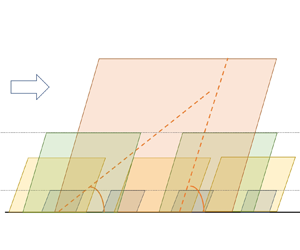
Figure 1. A schematic of the attached-eddy model: (a)  $x$–
$x$– $y$ plane view, and (b) $y$–
$y$– $z$ plane view. Each parallelogram in (a) and circle in (b) represents an individual attached eddy. Here, $x$,
$x$,  $y$ and $z$ denote the streamwise, wall-normal and spanwise directions, respectively. Also, $y_s^+$ ( $=100$) and $y_e^+$ ( $=0.2h^+$) denote the lower and upper bounds of the logarithmic region, respectively (Jiménez Reference Jiménez2018; Baars & Marusic Reference Baars and Marusic2020a; Wang, Hu & Zheng Reference Wang, Hu and Zheng2021); $y_o^+$ is the outer reference height; $\Delta y^+$ is the local grid spacing along the wall-normal direction; and $\alpha _m$ and $\alpha _s$ are the mean and individual SIA of attached eddies, respectively. These two diagrams are merely conceptual sketches, and the eddy population density is not in accordance with that of Perry & Chong (Reference Perry and Chong1982).
Previous studies have established that the energy-containing eddies populating the logarithmic and outer regions bear characteristic streamwise inclination angles (SIAs) due to the mean shear (see figure 1a). As early as the 1970s, Kovasznay, Kibens & Blackwelder (Reference Kovasznay, Kibens and Blackwelder1970) found that the large-scale structures in the outer intermittent region of a turbulent boundary layer have a moderate tilt in the streamwise direction. On the other hand, for the eddies in the logarithmic region of wall turbulence, the wall-attached  $\varLambda$-vortex was used by Perry & Chong (Reference Perry and Chong1982) to illustrate them. According to Adrian, Meinhart & Tomkins (Reference Adrian, Meinhart and Tomkins2000), these $\varLambda$-vortices are apt to cluster along the flow direction and form an integral whole (generally called vortex packets). Further observations in channel flows (Christensen & Adrian Reference Christensen and Adrian2001) demonstrated that the heads of $\varLambda$-vortices among the vortex packets tend to slope away from the wall in a statistical sense, with SIAs between $12^{\circ }$ and $13^{\circ }$. Most additional studies have shown a similar result, and it is accepted widely that the approximate SIAs of eddies are in the range $10^{\circ }$– $16^{\circ }$ (Boppe, Neu & Shuai Reference Boppe, Neu and Shuai1999; Christensen & Adrian Reference Christensen and Adrian2001; Carper & Porté-Agel Reference Carper and Porté-Agel2004; Marusic & Heuer Reference Marusic and Heuer2007; Baars, Hutchins & Marusic Reference Baars, Hutchins and Marusic2016). Besides, the SIA is also found to be Reynolds-number-independent (Marusic & Heuer Reference Marusic and Heuer2007).
However, the SIA estimated by experimentalists using the traditional statistical approach is indeed the mean structure angle (Marusic & Heuer Reference Marusic and Heuer2007; Deshpande, Monty & Marusic Reference Deshpande, Monty and Marusic2019). The common procedure to obtain the SIA is based on the calculation of the cross-correlation between the streamwise wall-shear stress fluctuation ( $\tau _x'$) and the streamwise velocity fluctuation ( $u'$) at a wall-normal position in the log region ( $y_o$). The cross-correlation can be expressed as
 \begin{equation} R_{\tau_x' u'}(\Delta x)=\frac{\langle\tau_x'(x)\,u'(x+\Delta x,y_o)\rangle}{\sqrt{\left\langle\tau_x'^{2}\right\rangle\left\langle u^{\prime 2}\right\rangle}}, \end{equation}
where  $\langle\, \cdot\, \rangle$ represents the ensemble temporal and spatial average, and $\Delta x$ is the streamwise delay. The SIA can be estimated by
 \begin{equation} \alpha_m=\arctan\left(\frac{y_o}{\Delta x_{p}}\right), \end{equation}
where  $\Delta x_{p}$ denotes the streamwise delay corresponding to the peak in $R_{\tau _x' u'}$. Considering that an array of wall-attached eddies with distinct wall-normal heights can convect simultaneously past the reference position $y_o$, $\alpha _m$ in (1.2) should be regarded as the mean angle of these eddies. Hence the subscript $m$ in (1.2) refers to ‘mean’.
To estimate the SIAs of the largest wall-attached eddies, Deshpande et al. (Reference Deshpande, Monty and Marusic2019) introduced a spanwise offset between the near-wall and logarithmic probes to isolate these wall-attached motions in the log region. They found that their SIAs are approximately  $45^{\circ }$. This observation is consistent with several theoretical analyses. For example, Moin & Kim (Reference Moin and Kim1985) and Perry, Uddin & Marusic (Reference Perry, Uddin and Marusic1992) proposed that for flows with two-dimensional mean flows, the characteristic angles of the energy-containing eddies should follow the direction of the principal rate of mean strain. More specifically, their SIAs should be $45^{\circ }$ for a zero-pressure-gradient turbulent boundary layer (Perry et al. Reference Perry, Uddin and Marusic1992). Marusic (Reference Marusic2001) found that the mean SIA of the induced turbulence field by attached eddies is akin to the experimental measurements if the hierarchical attached eddies tilt away from the wall with individual SIA $45^{\circ }$ and organize like the vortex packets observed in numerical and laboratory experiments.
Reviewing the work of predecessors, it can be found that the SIAs of attached eddies at a given length scale are ambiguous. Traditional measurements are applicable only for the assessment of the mean SIA (Brown & Thomas Reference Brown and Thomas1977; Boppe et al. Reference Boppe, Neu and Shuai1999; Marusic & Heuer Reference Marusic and Heuer2007). Moreover, the technique adopted by Deshpande et al. (Reference Deshpande, Monty and Marusic2019) can isolate only the largest wall-attached motions in the logarithmic region. Considering the characteristic scale of an individual attached eddy as its wall-normal height, as per the attached-eddy model (Townsend Reference Townsend1976; Perry & Chong Reference Perry and Chong1982), it is self-evident that it is of great importance to assess the SIAs of attached eddies with any heights in the logarithmic region, for not only the completeness of attached-eddy hypothesis, but also the accuracy of turbulence simulations (Marusic Reference Marusic2001; Carper & Porté-Agel Reference Carper and Porté-Agel2004). In the present study, we aim to achieve this goal by leaning upon the modified spectral stochastic estimation (SSE) proposed by Baars et al. (Reference Baars, Hutchins and Marusic2016), and dissecting the direct numerical simulations (DNS) database spanning broad-band Reynolds numbers. We will also discuss the relationship between the mean SIA and the scale-based SIA.
2. DNS database and methodology to calculate the SIA
2.1. DNS database
The DNS database adopted in the present study has been validated extensively by Jiménez and co-workers (Del Álamo & Jiménez Reference Del Álamo and Jiménez2003; Del Álamo et al. Reference Del Álamo, Jiménez, Zandonade and Moser2004; Hoyas & Jiménez Reference Hoyas and Jiménez2006; Lozano-Durán & Jiménez Reference Lozano-Durán and Jiménez2014). Four cases, at  $Re_\tau =545$, 934, 2003 and 4179, are used and named Re550, Re950, Re2000 and Re4200, respectively ( $Re_{\tau }=hu_{\tau }/\nu$, where $h$ denotes the channel half-height, $u_{\tau }$ the wall friction velocity and $\nu$ the kinematic viscosity). All these data are provided by the Polytechnic University of Madrid. Details of the parameter settings are listed in table 1. Note that the relatively smaller computational domain size of Re4200 may influence the estimation of SIAs of the attached eddies populating the upper part of the logarithmic region. This limitation will be discussed in § 3 and the Appendix.
Table 1. Parameter settings of the DNS database. Here,  $L_x$, $L_y$ and $L_z$ are the sizes of the computational domain in the streamwise, wall-normal and spanwise directions, respectively. Also, $\Delta x^+$ and $\Delta z^+$ denote the streamwise and spanwise grid resolutions in viscous units, respectively; $\Delta y_{min}^+$ and $\Delta y_{max}^+$ denote the finest and coarsest resolutions in the wall-normal direction, respectively; $N_F$ and $Tu_{\tau }/h$ indicate the number of instantaneous flow fields and the total eddy turnover time used to accumulate statistics, respectively.

2.2. Spectral stochastic estimation
According to the inner–outer interaction model (Marusic, Mathis & Hutchins Reference Marusic, Mathis and Hutchins2010), large-scale motions would exert footprints on the near-wall region, i.e. the superposition effects. Baars et al. (Reference Baars, Hutchins and Marusic2016) demonstrated that this component (denoted as  $u_{L}^{\prime +}(x^{+}, y^{+}, z^{+})$) can be obtained by the SSE of the streamwise velocity fluctuation at the logarithmic region $y_o^+$, namely by
 \begin{equation} u_{L}^{\prime +}\left(x^{+}, y^{+}, z^{+}\right)=F_{x}^{{-}1}\left\{H_{L}\left(\lambda_{x}^{+}, y^{+}\right) F_{x}\left[u_{o}^{\prime +}\left(x^{+}, y_{o}^{+}, z^{+}\right)\right]\right\}, \end{equation}
where  $u_{o}^{\prime +}$ is the streamwise velocity fluctuation at $y_o^+$ in the logarithmic region, and $F_x$ and $F_x^{-1}$ denote the fast Fourier transform (FFT) and the inverse FFT in the streamwise direction, respectively. Here, $H_L$ is the transfer kernel, which evaluates the correlation between $\widehat {u'}(y^+)$ and $\widehat {u_o'}(y_o^+)$ at a given length scale $\lambda _{x}^{+}$; it can be calculated as
 \begin{equation} H_{L}\left(\lambda_{x}^{+},y_o^{+}\right)=\frac{\left\langle\widehat{u'}\left(\lambda_{x}^{+}, y^{+}, z^{+}\right) \overline{\widehat{u_o'}}\left(\lambda_{x}^{+}, y_{o}^{+}, z^{+}\right)\right\rangle}{\left\langle\widehat{u_o'}\left(\lambda_{x}^{+}, y_{o}^{+}, z^{+}\right) \overline{\widehat{u_o'}}\left(\lambda_{x}^{+}, y_{o}^{+}, z^{+}\right)\right\rangle}, \end{equation}
where  $\widehat {u'}$ is the Fourier coefficient of $u'$, and $\overline {\widehat {u'}}$ is the complex conjugate of $\widehat {u'}$. Here, $y^+$ is set as $y^+=0.3$, and the outer reference height $y_o^+$ varies from $100$ to the outer region $0.7h^+$ according to the wall-normal grid distribution. Once $u_L^{\prime +}$ is obtained, the superposition component of $\tau _x^{\prime +}$ can be calculated by definition (i.e. ${\partial u_L^{\prime +}}/{ \partial y^+}$ at the wall) and denoted as $\tau _{x,L}^{\prime +}(y_o^+)$.
Analogously, to eliminate the effects from the wall-detached eddies with random orientations, which contribute significantly to the streamwise velocity fluctuations at  $y_o^+$, we can also use the near-wall streamwise velocity fluctuation in the viscous layer $y^+$ to reconstruct the wall-coherent streamwise velocity fluctuation in the logarithmic region $y_o^+$ by SSE (Adrian Reference Adrian1979), i.e.
 \begin{equation} u_{W}^{\prime +}\left(x^{+}, y_o^{+}, z^{+}\right)=F_{x}^{{-}1}\left\{H_{W}\left(\lambda_{x}^{+}, y^{+}\right) F_{x}\left[u^{\prime +}\left(x^{+}, y^{+}, z^{+}\right)\right]\right\}, \end{equation}
where  $u_{W}^{\prime +}$ is the wall-coherent component of $u_{o}^{\prime +}$. The wall-based transfer kernel $H_W$ can be calculated as
 \begin{equation} H_{W}\left(\lambda_{x}^{+},y_o^{+}\right)=\frac{\left\langle\widehat{u_o'}\left(\lambda_{x}^{+}, y_o^{+}, z^{+}\right) \overline{\widehat{u'}}\left(\lambda_{x}^{+}, y^{+}, z^{+}\right)\right\rangle}{\left\langle\widehat{u'}\left(\lambda_{x}^{+}, y^{+}, z^{+}\right) \overline{\widehat{u'}}\left(\lambda_{x}^{+}, y^{+}, z^{+}\right)\right\rangle}. \end{equation}
 Figure 2(a) shows the variation of  $\langle u_{W}^{\prime 2+} \rangle$ as a function of $y_o/h$ in the case Re2000. The full-channel data are included for comparison. It can be seen that $\langle u_{W}^{\prime 2+} \rangle$ follows roughly the logarithmic decay for $0.09\le y_o/h\le 0.2$, i.e. the logarithmic region. To quantify the logarithmic decay systematically, we define the indicator function $\varXi =y(\partial \langle u^{\prime 2+} \rangle /\partial y)$, and display its variations in figure 2(b). Comparing with the full-channel data, a comparatively well-defined plateau is observed for $\langle u_{W}^{\prime 2+} \rangle$. The logarithmic variance of $\langle u_{W}^{\prime 2+} \rangle$ shown in figure 2 is the consequence of the additive attached eddies (Townsend Reference Townsend1976), and can be expressed as
 \begin{equation} \langle u_{W}^{\prime 2+} \rangle=C_2-C_1\ln(y_o/h), \end{equation}
where  $C_2$ and $C_1$ are two constants, and $C_1$ is approximately equal to 0.54. Actually, the magnitude of the slope of the logarithmic decaying is affected by the Reynolds number, the configuration of the wall turbulence, the methodology for isolating the signals carried by the attached eddies, and the effects of the VLSMs. The indicator function $\varXi$ of the full-channel data shown in figure 2(b) suggests that the logarithmic region of case Re2000 is not fully developed, as the slope value of the logarithmic decaying is smaller than the Townsend–Perry constant $1.26$ reported in high-Reynolds-number experiments (Marusic et al. Reference Marusic, Monty, Hultmark and Smits2013), and close to the magnitude of $C_1$ observed here. Furthermore, Baars & Marusic (Reference Baars and Marusic2020b) reported that $C_1=0.98$ in turbulent boundary layers by analysing the streamwise velocity fluctuations carried by the attached eddies in the logarithmic region, while Hu, Yang & Zheng (Reference Hu, Yang and Zheng2020) and Hwang et al. (Reference Hwang, Lee and Sung2020) showed that $C_1=0.8$ and 0.37 in channel flows, respectively. Hu et al. (Reference Hu, Yang and Zheng2020) adopted a scale-based filter to extract the streamwise velocity fluctuations associated with the attached eddies in the logarithmic region, and did not take into account their imperfect coherence with the near-wall flow at each scale. The wall-based transfer kernel $H_W$ in (2.4) employed here can achieve this. Hwang et al. (Reference Hwang, Lee and Sung2020) utilized the three-dimensional clustering method to identify the wall-attached structures in a channel flow. The differences among these decomposition methodologies may be the reason why the magnitude of $C_1$ for turbulent channel flows reported by Hu et al. (Reference Hu, Yang and Zheng2020) and Hwang et al. (Reference Hwang, Lee and Sung2020) is not identical to that of the present study. Besides, it is noted that the effects of VLSMs are also retained in $\langle u_{W}^{\prime 2+} \rangle$, and their impacts on the logarithmic decaying are non-negligible. By the way, the methodology introduced in § 2.3 to estimate the SIAs of attached eddies at a single scale can effectively diminish the effects originating from the VLSMs (see figure 4). In summary, these observations demonstrate that $u_{W}'$ can be considered as approximately the streamwise velocity fluctuations carried by the multi-scale wall-attached eddies. We will focus on the statistics in the logarithmic region in the following sections.

Figure 2. (a) Variations of the statistic  $\langle u_{W}^{\prime 2+} \rangle$ as a function of $y_o/h$, with the full-channel data $\langle u^{\prime 2+} \rangle$ included for comparison. (b) Variations of the indicator function $\varXi$ as functions of $y_o/h$. The red line in (a) denotes the logarithmic decaying (2.5) with $C_1=0.54$. The data is taken from the case Re2000.
2.3. Methodology to isolate targeted eddies
Apparently, the SIAs of attached eddies at a single scale ( $\alpha _s$) cannot be pursued by (1.1)–(1.2). It is worth noting that in (1.1)–(1.2), the input parameter and signals are $y_o$, $\tau _x'$ and $u'(y_o)$. Thus to obtain an accurate $\alpha _s$, $y_o$ should be set reasonably, and $\tau _x'$ and $u'(y_o)$ should also be processed properly, to characterize the properties of the attached eddies at the targeted scale. Our new approach is based on this understanding.
According to the hierarchical distribution of the multi-scale attached eddies in high-Reynolds-number wall turbulence (see figure 1(b), also figure 14 of Perry & Chong Reference Perry and Chong1982),  $\tau _{x,L}^{\prime +}(y_o^+)$ represents the superposition contributed from the wall-attached motions with their height larger than $y_o^+$. Thus, the difference value $\Delta \tau _{x,L}^{\prime +}(y_o^+)=\tau _{x,L}^{\prime +}(y_o^+)-\tau _{x,L}^{\prime +}(y_o^++\Delta y^+)$ can be interpreted as the superposition contribution generated by the wall-attached eddies with their wall-normal heights between $y_o^+$ and $y_o^++\Delta y^+$. Here, $y_o^++\Delta y^+$ is the location of the wall-normal grid cell adjacent to that at $y_o^+$, as $\Delta y^+$ is the local grid spacing along the wall-normal direction, in viscous units, determined by the simulation set-ups. A similar numerical framework has been verified by our previous study (Cheng & Fu Reference Cheng and Fu2022). Correspondingly, the difference value $\Delta u_{W}^{\prime +}(y_o^+)=u_{W}^{\prime +}(y_o^+)-u_{W}^{\prime +}(y_o^++\Delta y^+)$ is the streamwise velocity fluctuation carried by attached eddies populating the region between $y_o^+$ and $y_o^++\Delta y^+$. In this way, the SIAs of these eddies can be assessed by
 \begin{equation} \alpha_s(y_m)=\arctan\left(\frac{y_m}{\Delta x_{p}}\right), \end{equation}
where  $y_m=({y_o+(y_o+\Delta y)})/{2}$, and $\Delta x_{p}$ is the streamwise delay associated with the peak of the cross-correlation
 \begin{equation} R_{LW}(\Delta x)=\frac{\langle\Delta \tau_{x,L}^{\prime +}(x,y_o^+)\,\Delta u_{W}^{\prime +}(x+\Delta x,y_o^+)\rangle}{\sqrt{\left\langle\Delta \tau_{x,L}^{\prime 2+}\right\rangle\left\langle \Delta u_{W}^{\prime 2+}\right\rangle}}. \end{equation}
 As the statistical characteristics of an individual attached eddy being self-similar with its wall-normal height as per the attached-eddy hypothesis (Townsend Reference Townsend1976),  $y_m$ is just the characteristic scale of the wall-attached motions within $y_o^+$ and $y_o^++\Delta y^+$. Figure 3 shows the variations of $\Delta y^+$ as functions of $y_o^+$ in the logarithmic region for all cases. It can be seen that the maximum values of $\Delta y^+$ are less than 7 in the case Re4200. In this regard, treating $y_m$ as the mean height of the attached eddies populating the region between $y_o$ and $y_o+\Delta y$ is reasonable, as the zone between $y_o$ and $y_o+\Delta y$ is narrow compared to the spanning of the logarithmic region. The new procedure isolates the attached eddies at a given scale from the rest of the turbulence. The cross-correlation, i.e. (2.7), gets rid of the influences originated from other scales, and preserves the phase information of the wall-attached motions with wall-normal height $y_m$.

Figure 3. Variations of  $\Delta y^+$ as functions of $y_o^+$ in the logarithmic region for all cases.

Figure 4. Streamwise premultiplied spectra of  $\Delta \tau _{x,L}'$, $\Delta u_{W}'$, $\tau _{x}'$ and $u'$ for (a) $y_o=0.1h$, and (b) $y_o=0.2h$, in the case Re2000. Each spectrum is normalized with its maximum value. The vertical dashed lines are plotted to highlight the corresponding $\lambda _x/h$ of the maximum values of the premultiplied spectra of $\Delta \tau _{x,L}'$ and $\Delta u_{W}'$.
Finally, the critical assumptions of the present approach and its realization merit a discussion. Our methodology is based on the hierarchical distribution of the attached eddies, and the hypothesis that the characteristic velocity scales carried by the attached eddies with different wall-normal heights are identical with their scale interactions omitted. That is, the attached eddies in each hierarchy contribute equally to the streamwise wall-shear fluctuations on the wall surface and the streamwise turbulence intensity in the lower bound of the logarithmic region. Only in this way, both  $\Delta \tau _{x,L}^{\prime +}$ and $\Delta u_{W}^{\prime +}$ reflect approximately the characteristics of the attached eddies at $y_m$. In fact, these assumptions are also the key elements when developing the attached-eddy model (Townsend Reference Townsend1976; Perry & Chong Reference Perry and Chong1982; Woodcock & Marusic Reference Woodcock and Marusic2015; Yang, Marusic & Meneveau Reference Yang, Marusic and Meneveau2016; Mouri Reference Mouri2017; Yang & Lozano-Durán Reference Yang and Lozano-Durán2017), and some of them may be valid only in high-Reynolds-number wall turbulence. For example, the hierarchical distribution of the multi-scale attached eddies is prominent at high-Reynolds-number turbulence (De Silva, Marusic & Hutchins Reference De Silva, Marusic and Hutchins2016; Cheng et al. Reference Cheng, Li, Lozano-Durán and Liu2019; Marusic & Monty Reference Marusic and Monty2019). However, when the DNS data listed in table 1 are utilized to study the characteristics of the attached eddies, the finite Reynolds number effects and the intricate scale interactions would take effect inevitably. Besides, the VLSMs, which cannot be depicted by the attached-eddy model, would also impose non-trivial impacts (Perry & Marusic Reference Perry and Marusic1995; Baars & Marusic Reference Baars and Marusic2020a; Hwang et al. Reference Hwang, Lee and Sung2020). Accordingly, the subtraction between $u_{W}^{\prime +}(y_o^+)$ and $u_{W}^{\prime +}(y_o^++\Delta y^+)$ cannot achieve a sharp cut-off at the targeted scale in the spectral space, and hereby the spectrum of $\Delta u_{W}^{\prime +}(y_o^+)$ would be comparatively small but not negligible at the smaller and larger scales of the targeted one. The finiteness of $\Delta y^+$ is another factor, which is worth attention in some scenarios. Due to the limitations of numerical simulation, $\Delta y^+$ is a finitely small quantity. When assessing the SIA of the attached eddies at a given wall-normal height, treating $y_m^+$ as their characteristic scales (therefore neglecting the effects of the narrow band between $y^+$ and $y^++\Delta y^+$) is acceptable, because $\Delta y^+$ is rather small compared to the spanning of the whole logarithmic region. The linear growth of the typical length scales of $\Delta \tau _{x,L}^{\prime +}$ and $\Delta u_{W}^{\prime +}$ shown in figure 6(b) can verify this validity. On the other hand, when the spectral characteristics of $\Delta u_{W}^{\prime +}$ are considered, $\Delta u_{W}^{\prime +}$ should be interpreted as the additive outcomes of the attached eddies with their wall-normal heights within $y^+$ and $y^++\Delta y^+$, strictly speaking. Under these circumstances, the spectral energy distribution that corresponds to the self-similar attached eddies within this range should be observed to peak around the dominant wavelength, and vary continuously and locally. The results shown in figure 5 confirm our proposition. Details will be discussed in the next section.

Figure 5. Premultiplied one-dimensional streamwise spectra of  $\Delta u_{W}'$ around (a) $y_o=0.05h$, (b) $y_o=0.1h$, in Re2000. The horizontal dashed lines represent the plateaus or peaks of the spectra. The vertical lines are plotted to highlight the self-similar regions of each spectrum.

Figure 6. (a) Variations of  $R_{\Delta u_{W,p}'\,\Delta u_{W,p}'}$ as functions of $\Delta x/h$ for two selected $y_o$. (b) Variations of $\Delta s/h$ as functions of $y_m^+$ for $\Delta \tau _{x,L,p}^{\prime +}$ and $\Delta u_{W,p}^{\prime +}$. The line in (b) denotes the linear variation $2\Delta s=10.8y_m$. The data is taken from the case Re2000.
3. Results
Before investigating the SIAs of attached eddies, it is important to study the characteristic scales of  $\Delta \tau _{x,L}'$ and $\Delta u_{W}'$ first. Figures 4(a,b) show their streamwise premultiplied spectra at $y_o=0.1h$ and $y_o=0.2h$, respectively, for Re2000. The spectra of $\tau _{x}'$ and $u'$ of the full-channel data are also included for comparison. Each spectrum is normalized with its maximum value. It can be seen that the spectra of $\Delta \tau _{x,L}'$ and $\Delta u_{W}'$ are roughly coincident, and peak at $\lambda _x=2.1h$ for $y=0.1h$, and $\lambda _x=4.2h$ for $y=0.2h$, respectively. By contrast, the spectra of $\tau _{x}'$ and $u'$ do not share similar spectral characteristics. It is noted that $\Delta u_{W}^{\prime 2}$ and $\Delta \tau _{x,L}^{\prime 2}$ account for very little energy of the full-channel signals at the same wall-normal positions. For example, $\Delta u_{W}^{\prime 2}$ at $y_o=0.1h$ and $0.2h$ occupies 0.0034 $\%$ and 0.002 $\%$ of $u^{\prime 2}$ at the corresponding positions, whereas $\Delta \tau _{x,L}^{\prime 2}$ for $y_o=0.1h$ and $0.2h$ occupies 0.012 $\%$ and 0.0045 $\%$ of $\tau _{x}^{\prime 2}$, respectively. Moreover, comparing with the spectra of the full-channel data, the spectra of $\Delta u_{W}'$ decay rapidly when $\lambda _x\geq 4h$ (see figure 4), which indicates that the effects of VLSMs on $\Delta u_{W}'$ are rather limited.
Figure 5 shows the streamwise premultiplied spectra of  $\Delta u_{W}'$ around $y_o=0.05h$ and $y_o=0.1h$. Each spectrum is normalized by the energy of $\Delta u_{W}'$ at a given $y_m$. Clear plateau regions can be observed around the spectral peaks. For $y_o=0.05h$, the region is $18\le \lambda _x/y_m \le 30$, and for $y_o=0.1h$ it is $17\le \lambda _x/y_m \le 31$ , which corresponds to the $k_x^{-1}$ region in the spectrum predicated by the attached-eddy model, and can be considered as the spectral signatures of the attached eddies (Perry & Chong Reference Perry and Chong1982; Perry, Henbest & Chong Reference Perry, Henbest and Chong1986; Hwang et al. Reference Hwang, Lee and Sung2020; Deshpande, Monty & Marusic Reference Deshpande, Monty and Marusic2021). Besides, the spectra shown here resemble the spectrum of the type A eddies hypothesized by Marusic & Perry (Reference Marusic and Perry1995), i.e. the energy fraction captured by the attached-eddy model. These observations support the proposition that the $\Delta u_{W}'$ signals are the streamwise velocity fluctuations carried by the self-similar attached eddies predominantly. Moreover, they also indicate that the streamwise length scales of the dominant eddies increase with $y_o$, as the self-similar range is not altered significantly with increasing $y_o$.
To investigate further the scale characteristics of  $\Delta \tau _{x,L}'$ and $\Delta u_{W}'$, we consider the autocorrelation function of $\Delta u_{W,p}^{\prime +}$ (the signals that are extracted from the spectral peaks shown in figure 5, i.e. filtered $\Delta u_{W}'$ with wavelength larger than $17y_m$, but smaller than $31y_m$), which takes the form
 \begin{equation} R_{\Delta u_{W,p}'\Delta u_{W,p}'}(\Delta x,y_o)=\frac{\langle\Delta u_{W,p}^{\prime}\left(x, y_o, z\right)\Delta u_{W,p}^{\prime}\left(x+\Delta x, y_o, z\right)\rangle }{\langle\Delta u_{W,p}^{\prime 2}\left(x, y_o, z\right)\rangle}, \end{equation}
and the counterpart of  $\Delta \tau _{x,L}^{\prime +}$ can be defined similarly. Figure 6(a) shows the variations of $R_{\Delta u_{W,p}'\Delta u_{W,p}'}$ as functions of $\Delta x/h$ for two selected $y_o$ values. The larger $y_o$, the broader is $R_{\Delta u_{W,p}'\Delta u_{W,p}'}$. As a measure of the typical length scale, we employ $\Delta s/h$, which is the streamwise delay corresponding to $R_{\Delta u_{W,p}'\Delta u_{W,p}'}=0.05$ or $R_{\Delta \tau _{x,L,p}'\Delta \tau _{x,L,p}'}=0.05$ (here, 0.05 is an empirical small positive threshold). Figure 6(b) shows the variations of $2\Delta s/h$ as functions of $y_m/h$ for $\Delta \tau _{x,L,p}^{\prime +}$ and $\Delta u_{W,p}^{\prime +}$. For both $\Delta \tau _{x,L,p}^{\prime +}$ and $\Delta u_{W,p}^{\prime +}$, $2\Delta s/h$ increases linearly with $y_m/h$ throughout most of the logarithmic region. This observation is consistent with the attached-eddy hypothesis, which states that the length scales of the attached eddies grow linearly with their wall-normal heights (Hwang Reference Hwang2015; Marusic & Monty Reference Marusic and Monty2019). Moreover, both the streamwise length scales of $\Delta \tau _{x,L,p}^{\prime +}$ and $\Delta u_{W,p}^{\prime +}$ follow $2\Delta s=10.8y_m$ (considering the symmetry of the autocorrelation function with respect to $\Delta x=0$, $2\Delta s$ truly represents the streamwise length scale of the signals). This scale characteristic agrees well with some previous studies. For example, Baars, Hutchins & Marusic (Reference Baars, Hutchins and Marusic2017) showed that the streamwise/wall-normal aspect ratio of the wall-attached eddy structure is $\lambda _x/y=14$ in turbulent boundary layers, which is close to the result here. Hwang et al. (Reference Hwang, Lee and Sung2020) reported that the spectra of the self-similar wall-attached structures agree with the attached-eddy hypothesis at $\lambda _x=12y$, which is consistent with the estimation of the present study. All these observations indicate that $\Delta \tau _{x,L}^{\prime +}$ and $\Delta u_{W}^{\prime +}$ are representative of the attached eddies at a certain wall-normal height, though the minor influences of VLSMs still exist, and treating $y_m^+$ as their characteristic scales is reasonable.
In summary, all the observations mentioned above indicate that  $\Delta \tau _{x,L}'$ and $\Delta u_{W}'$ are the outcomes of the energy-containing motions with the wall-normal heights approximately equal to $y_m$, and the cross-correlation, i.e. (2.7), truly reflects the phase difference between the streamwise velocity fluctuations carried by these motions and their footprints in the near-wall region. Other wall-normal positions and DNS cases yield similar results and are not shown here for brevity.
Figure 7(a) shows the variations of  $R_{LW}$ as functions of the streamwise delay for some selected wall-normal positions in the case Re2000. Since the streamwise length scales of the energy-containing motions are increased with their normal heights (see figure 4), $R_{LW}$ becomes wider about the peak with increasing $y_o$. We can identify $\Delta x_{p}$ obviously from the cross-correlation profiles, and the SIAs of the attached eddies at a given wall-normal height can be calculated according to (2.6). Figure 7(b) plots the variations of the normalized $R_{LW}$ as functions of $\Delta x/y_m$ for some selected $y_o$ in the case Re2000. The $R_{LW}$ distributions are normalized with their maximum values $R_{LW,max}$. It can be seen that the profiles of $R_{LW}/R_{LW,max}$ for different wall-normal heights coincide well with each other, which indicates the self-similar characteristics of the energy-containing motions in the logarithmic region. We have checked that the correlations calculated from the raw data, i.e. $R_{\tau _x' u'}$ in (1.1), cannot coincide if normalized in this manner. Again, it demonstrates that the new methodology is capable of capturing the main properties of the attached eddies.

Figure 7. (a) Variations of  $R_{LW}$, i.e. the cross-correlation between $\Delta \tau _{x,L}^{\prime +}(y_o^+)$ and $\Delta u_{W}^{\prime +}(y_o^+)$, as functions of $\Delta x/h$ for some selected $y_o$ values in the case Re2000. (b) Variations of the normalized $R_{LW}$ as functions of $\Delta x/y_m$ for some selected $y_o$ values in the case Re2000. The $R_{LW}$ profiles are normalized with their maximum values in (b). The vertical dashed lines in (a) are plotted to highlight the maximum values of $R_{LW}$ and their corresponding $\Delta _x/h$.
Figure 8 plots the variations of  $\alpha _s$ as functions of $y_m^+$ for all cases; approximately, $\alpha _s$ increases from $27^{\circ }$ for Re550, to $40^{\circ }$ for Re4200. For a given case, $\alpha _s$ changes little spanning the logarithmic region except for the upper part of the logarithmic region in Re4200. Deshpande et al. (Reference Deshpande, Monty and Marusic2019) isolated the large wall-attached structures in a DNS of turbulent boundary layer at $Re_{\tau }\approx 2000$, and found the corresponding SIAs to be $32^{\circ }$ (see figure 4(a) of their paper). Their observation is consistent with the results of the present study. However, Deshpande et al. (Reference Deshpande, Monty and Marusic2019) calculated only the SIAs of the largest wall-attached motions in the logarithmic region, due to the limitation of the methodology adopted in their study, whereas we make a thorough investigation on the SIAs of attached eddies with any wall-normal heights in the logarithmic region. Moreover, Deshpande et al. (Reference Deshpande, Monty and Marusic2019) reported that the SIAs of the large wall-attached motions identified in a wind-tunnel boundary layer with $Re_{\tau }=14000$ are approximately $50^{\circ }$. They ascribed the result difference between DNS and experiment to the limited streamwise scale range owing to the DNS domain size selected for analysis. Our results reveal that the Reynolds number effects play a non-negligible role in the formation of SIAs of attached eddies. To the authors’ knowledge, this is the first time that the Reynolds number dependence of SIAs of the wall-attached motions at a given length scale has been shown clearly. Finally, it should be noted that $\alpha _s$ of Re4200 decreases rapidly for $y_m^+>500$ (not shown here). This diversity is due to the small computational domain size along the streamwise direction in this database. Thus in the discussion below, the statistics of $\alpha _s$ in the range $y_m^+>500$ in Re4200 will not be taken into account. The sensitivity of the presented results to the number of instantaneous flow fields employed for accumulating statistics is examined in the Appendix.

Figure 8. Variations of  $\alpha _s$ as functions of $y_m^+$ for all cases. The red dashed lines denote the mean $\alpha _s$ across the logarithmic region of each case.
Figure 9(a) shows the mean  $\alpha _s$ ( $\alpha _{s,m}$) distribution in the range of the logarithmic region as a function of the friction Reynolds number. It can be seen that the SIA may reach the theoretical prediction angle $45^{\circ }$ (Perry et al. Reference Perry, Uddin and Marusic1992) when $Re_{\tau } \sim O(10^4)$. The results of DNS of a turbulent boundary layer and wind-tunnel experiment of Deshpande et al. (Reference Deshpande, Monty and Marusic2019) roughly agree with the tendency. The minor differences may result from the distinct configurations of the wall-bounded turbulence.

Figure 9. (a) Variations of the mean  $\alpha _s$ ( $\alpha _{s,m}$) statistic in the range of logarithmic region as a function of the friction Reynolds number; the experimental results of turbulent boundary layers (Deshpande et al. Reference Deshpande, Monty and Marusic2019) are also included for comparison. (b) Variations of $\alpha _{m}$ and $\alpha _{SSE,m}$ as functions of $y_o^+$ for Re2000. The solid black line in (a) denotes the theoretical prediction angle $45^{\circ }$, and the dashed line in (a) indicates the asymptotic behaviour of $\alpha _{s,m}$.
4. Discussion
4.1. Effects of near-wall and detached motions
To clarify the effects of near-wall and detached motions on the SIA assessment, we calculate the mean SIA based on the predictive signals, i.e.
 \begin{equation} \alpha_{SSE,m}=\arctan\left(\frac{y_o}{\Delta x_{p}}\right), \end{equation}
where  $\Delta x_{p}$ is the streamwise delay associated with the peak of the cross-correlation
 \begin{equation} R_{\tau_{x,L}' u_W'}(\Delta x)=\frac{\langle\tau_{x,L}'(x)\,u_W'(x+\Delta x,y_o)\rangle}{\sqrt{\left\langle\tau_{x,L}^{\prime 2}\right\rangle\left\langle u_W^{\prime 2}\right\rangle}}. \end{equation}
 Figure 9(b) shows the variations of  $\alpha _{SSE,m}$ as a function of $y_o^+$ for Re2000, and the statistics of $\alpha _{m}$ are also included for comparison. We can see that the $\alpha _{SSE,m}$ distribution is very closed to that of $\alpha _{m}$. It highlights the fact that the phase information embedded in the raw signals $u'(y_o^+)$ and $\tau _{x}'$ is preserved by SSE. It also suggests that the near-wall and wall-detached motions, which cannot be captured by SSE, have a negligible impact on the magnitudes of SIA.
4.2.  $\alpha _s$ versus $\alpha _m$


Reviewing the approach to obtain the  $\alpha _m$ (i.e. (1.1)–(1.2)), the proposition that $\alpha _m$ is the mean SIA of attached eddies manifests in three aspects. ( $1$) the generation of $\tau _{x}'$ is not only the outcome of the near-wall motions, but also the footprints of all the wall-attached eddies (Cho, Hwang & Choi Reference Cho, Hwang and Choi2018; Cheng et al. Reference Cheng, Li, Lozano-Durán and Liu2020a). ( $2$) In the logarithmic region, $u'$ results from a sum of random contributions from the wall-attached eddies with distinct characteristic length scales (Yang et al. Reference Yang, Marusic and Meneveau2016), and a portion of contributions from the wall-detached eddies (Baars & Marusic Reference Baars and Marusic2020b). ( $3$) Here, $y_o$ is a wall-normal position located in the logarithmic region and chosen arbitrarily. As mentioned above, an array of wall-attached eddies with distinct wall-normal heights can convect simultaneously past this reference position.
Here, an additive SIA is calculated to highlight the relationship between  $\alpha _s$ and $\alpha _m$, namely,
 \begin{equation} \alpha_{add}=\arctan\left(\frac{y_s}{\Delta x_{p}}\right), \end{equation}
where  $y_s^+=100$ is the lower boundary of the logarithmic region, and $\Delta x_{p}$ is the streamwise delay associated with the peak of the cross-correlation
 \begin{equation} R_{add}(\Delta x)=\frac{\langle(\tau_{x,L}^{\prime +}(x,y_s^+)-\tau_{x,L}^{\prime +}(x,y_o^+)) (u_{W}^{\prime +}(x+\Delta x,y_s^+)-u_{W}^{\prime +}(x+\Delta x,y_o^+))\rangle}{\sqrt{\left\langle(\tau_{x,L}^{\prime +}(x,y_s^+)-\tau_{x,L}^{\prime +}(x,y_o^+))^{2}\right\rangle\left\langle (u_{W}^{\prime +}(x ,y_s^+)-u_{W}^{\prime +}(x,y_o^+))^{2}\right\rangle}}, \end{equation}
where the reference position  $y_o^+$ varies from $y_s^++\Delta y^+$ (equal to 104) to $0.7h^+$. Figure 10(a) shows the variations of $\alpha _{add}$ as a function of $y_o^+$ for Re2000. It can be seen that $\alpha _{add}$ decreases from $37.8^{\circ }$ to $14^{\circ }$ as $y_o^+$ increases, which corresponds to $\alpha _{s} (y_m^+=102)$ and $\alpha _{m} (y_o^+=100)$, respectively. In other words, $\alpha _{add}$ converges from the SIAs of attached eddies with wall-normal height approximately $100$ in viscous units to the mean SIA at $y_o^+=100$. This observation can be explained through the prism of the hierarchical attached eddies in high-Reynolds-number wall turbulence. The increase of $y_o^+$ indicates that $\tau _{x,L}^{\prime +}(y_s^+)-\tau _{x,L}^{\prime +}(y_o^+)$ and $u_{W}^{\prime +}(y_s^+)-u_{W}^{\prime +}(y_o^+)$ are contributed by more and more wall-attached eddies with their normal heights larger than $y_s^+$, and gradually become equal to $\tau _{x,L}^{\prime +}(y_s^+)$ and $u_{W}^{\prime +}(y_s^+)$, respectively, when $y_o^+$ approaches $h^+$. Thus $R_{add}$ would also converge gradually to $R_{\tau _{x,L}' u_W'}$ in (4.2), and $\alpha _{add}$ converges to $\alpha _{m}$ and $\alpha _{SSE,m}$ concurrently.

Figure 10. (a) Variations of the additive SIA  $\alpha _{add}$ as a function of $y_o^+$ for Re2000. (b) The mean SIAs $\alpha _m$ as functions of $y_o^+$ for all cases.
Additionally, this study helps us to understand the variation tendency of  $\alpha _{m}$. Figure 10(b) plots the variations of $\alpha _{m}$ for all cases. It is observed clearly that $\alpha _{m}$ increases continuously with $y_o^+$. Taking Re2000 as an example, $\alpha _{m}$ increases from $14^{\circ }$ for $y_s^+$ to $15.3^{\circ }$ for $y_e^+$. Increasing $y_o^+$ implies that fewer and fewer wall-attached eddies contribute to $u'$. In this way, $\alpha _{m}$ would converge to $\alpha _{s}$ as $y_o^+$ increases, albeit more slowly.
4.3. Scale-dependent inclination angles of wall-attached eddies
An alternative approach for calculating the scale-dependent inclination angle (SDIA) has been reported by Baars et al. (Reference Baars, Hutchins and Marusic2016). The following are the primary processes and outcomes. The scale-specific phase between  $u'$ at $y^+$ and $y_o^+$ can be estimated as
 \begin{equation} \varPhi( \lambda_{x})=\arctan\left\{\frac{\operatorname{Im}\left[\phi_{u_{o}' u_{}'}\left(\lambda_{x},y^+,y_o^+\right)\right]}{\operatorname{Re}\left[\phi_{u_{o}' u_{}'}\left(\lambda_{x},y^+,y_o^+\right)\right]}\right\}, \end{equation}
where Im $(\,\cdot\, )$ and Re $(\,\cdot\, )$ denote the imaginary and real parts of $\phi _{u_{o}' u_{}'}$, namely, the numerator of (2.2). The scale-dependent streamwise shift can be calculated as
 \begin{equation} l(\lambda_{x})=\frac{\varPhi( \lambda_{x})\,\lambda_{x}}{2{\rm \pi}}. \end{equation}
Accordingly, the SDIA can be estimated as
 \begin{equation} \alpha_{sd}(\lambda_{x})=\arctan\left(\frac{y_o-y}{l(\lambda_{x})}\right). \end{equation}
A positive  $\alpha _{sd}$ value corresponds to a spatially forward-leaning structure.
Figure 11 shows the SDIAs as functions of  $\lambda _{x}/y_o$ for three selected wall-normal positions in the case Re2000. For $\lambda _{x}/y_o>18$, the SDIAs of the large-scale motions are shown to be approximately equal to $14^{\circ }$. (in fact, this is not the real SIA of the large-scale wall-attached structures, according to the study of Deshpande et al. Reference Deshpande, Monty and Marusic2019.) However, for the smaller length scales, the SDIAs tend to be negative and vary rapidly with $\lambda _{x}/y_o$. This is the range of self-similar structures reported by previous studies, especially those with $\lambda _x/y_o=14$ (Baars et al. Reference Baars, Hutchins and Marusic2017; Baidya et al. Reference Baidya2019). Similar results have also been reported by Baars et al. (Reference Baars, Hutchins and Marusic2016) (see figure 5 of their paper). It indicates that the phase spectrum shown in figure 11 cannot be interpreted with any physical relevance at these scales, as the scale-specific phases of them are random indeed. The contamination from the detached eddies with random orientations could be the source of this problem. This is the main purpose of the present study, i.e. to eliminate the corruption caused by the wall-detached motions and measure appropriately the SIAs of the wall-attached eddies at a certain wall-normal height.

Figure 11. Variations of the scale-dependent inclination angles for three selected wall-normal positions in the case Re2000. The vertical line denotes  $\lambda _{x}/y_o=14$.
5. Concluding remarks
In the present study, we develop a methodology to assess the streamwise inclination angles of the wall-attached eddies at a given wall-normal height in turbulent channel flows, by coupling the spectral stochastic estimation with the attached-eddy hypothesis. Our results show, for the first time, that the SIAs of the attached eddies are Reynolds-number-dependent in low and medium Reynolds numbers, and tend to be consistent with the theoretical prediction (i.e.  $\alpha _{s}=45^{\circ }$) as Reynolds number increases. We further reveal that the mean SIA reported by vast previous studies are the outcomes of the additive effect contributed by multi-scale attached eddies.
The attached-eddy model has been the guidance for the reconstruction of the velocity field in wall turbulence (Perry & Marusic Reference Perry and Marusic1995; Baidya et al. Reference Baidya, Philip, Hutchins, Monty and Marusic2017; Chandran et al. Reference Chandran, Baidya, Monty and Marusic2017). Hierarchical vortex packets that consist of  $\varLambda$-vortices with $\alpha _{s}=45^{\circ }$ are distributed on the wall surface to mimic the attached eddies. The present results suggest that a lower SIA of representative structures might be helpful for a more accurate reconstruction when the Reynolds number is not high enough. Moreover, within the state-of-the-art wall-modelled large-eddy simulation (WMLES) framework, one may estimate the instantaneous $\tau _{x}$ based on the velocities carried by the log region eddies (Fu et al. Reference Fu, Karp, Bose, Moin and Urzay2021; Fu, Bose & Moin Reference Fu, Bose and Moin2022). The Reynolds number dependence of SIAs of these eddies should be accounted for by an advanced model in this sense.
Acknowledgements
We would like to thank Professor Jiménez for making the DNS data available. We also express our gratitude to the reviewers of this paper for their kind and constructive comments.
Funding
L.F. acknowledges the fund from CORE as a joint research centre for ocean research between QNLM and HKUST, and the fund from Guangdong Basic and Applied Basic Research Foundation (no. 2022A1515011779).
Declaration of interests
The authors report no conflict of interest.
Appendix. Statistic sensitivity to $N_F$

The influences of the number of instantaneous flow fields for accumulating statistics are examined. Figure 12 shows the effect of  $N_F$ on the statistic $\alpha _s$ for the cases Re2000 and Re4200. Alteration of the statistical samples mainly affects the relative standard deviations (RSDs) of the results. To be specific, when $N_F$ increases from $48$ to $94$, RSD decreases from $3.9\,\%$ to $3.3\,\%$ for Re2000; but for Re4200, RSD decreases from $6.5\,\%$ to $3.7\,\%$ when $N_F$ increases from $20$ to $40$. Given the fact that the case Re4200 has limited domain size, raising $N_F$ can effectively reduce the wiggles in the outputs. Nevertheless, the mean value of $\alpha _s$ in the logarithmic region seems to be insensitive to $N_F$.

Figure 12. Plots of  $\alpha _s$ as functions of $y_m^+$ for the cases Re2000 and Re4200 with different $N_F$. The dashed lines denote the mean value of $\alpha _s$ in the logarithmic region.


 Open access