


1. Introduction
Across the world's oceans, variations in seawater temperature and salinity stratify the water column, producing conditions where density disturbances can propagate as internal waves. A key aim in physical oceanography is the untangling of processes responsible for the global cascade of energy from planetary-scale mechanical energy inputs (wind and the tides), to dissipation at the Kolmogorov scale. The generation and subsequent degeneration of these internal waves is a key process in this global cascade (Lamb Reference Lamb2014; Sarkar & Scotti Reference Sarkar and Scotti2017).
Internal solitary waves (ISWs) are a particular form of internal waves that have amplitude comparable to the pycnocline thickness, and often the overall depth of the water column (e.g. Grue et al. Reference Grue, Jensen, Rusås and Sveen1999). They are characterised by a balance of nonlinear steepening and wave dispersion, and as a result are able to travel large distances without significant change of form or magnitude. ISWs are found commonly across the world's oceans, and they maintain high levels of research interest due to their effectiveness in transporting energy and scalar properties (Helfrich & Melville Reference Helfrich and Melville2006), and for mixing in the ocean (e.g. Huang et al. Reference Huang, Chen, Zhao, Zheng, Zhou, Yang and Tian2016; Boegman & Stastna Reference Boegman and Stastna2019). Typically, internal waves are generated on density interfaces in stably stratified fluids by barotropic motion over topography such as sills, slopes and the shelf edge (e.g. Grue Reference Grue2005; da Silva, Buijsman & Magalhaes Reference da Silva, Buijsman and Magalhaes2015; Rayson, Jones & Ivey Reference Rayson, Jones and Ivey2019), with the evolution of the barotropic internal tide motion into far-field mode-1 and higher-mode ISWs being determined by nonlinear steepening mechanisms (Rayson et al. Reference Rayson, Jones and Ivey2019).
Whilst ISWs can travel considerable distance over a flat bottom without change of form, under certain conditions, such as when shoaling, their form can change considerably. As they do so, dissipation produced by the motion of breaking waves, both in the benthic boundary layer (BBL) and the pycnocline, is identified as a key process in the global cascade of energy from global-scale mechanical forcing to dissipation (St Laurent et al. Reference St Laurent, Simmons, Tang and Wang2011; Sarkar & Scotti Reference Sarkar and Scotti2017). Yet, these breaking processes remain poorly parameterised and understood (Lamb Reference Lamb2014; Boegman & Stastna Reference Boegman and Stastna2019). Breaking ISWs are also known to induce considerable vertical mixing of heat, nutrients and other scalar properties. Benthic ecosystems such as coral reefs benefit from upwelling of cold, nutrient-rich deep waters as a result of internal bores produced by the ISWs (Green et al. Reference Green, Jones, Rayson, Lowe, Bluteau and Ivey2019), whilst the change to the thermal environment these waves produce may increase reef resilience to climate change (Reid et al. Reference Reid, DeCarlo, Cohen, Wong, Lentz, Safaie, Hall and Davis2019).
In the field, ISWs of depression shoaling over gentle slopes have frequently been observed evolving into a train of ISWs of elevation (e.g. Orr & Mignerey Reference Orr and Mignerey2003; Shroyer, Moum & Nash Reference Shroyer, Moum and Nash2009; St Laurent et al. Reference St Laurent, Simmons, Tang and Wang2011). Although these same geophysically realistic slopes are typically difficult to replicate in the laboratory, or in numerical models, laboratory experiments in an 18 m wave tank identified the formation of boluses propagating up-slope from the evolution of periodic waves propagating over gentle slopes (Wallace & Wilkinson Reference Wallace and Wilkinson1988). Additionally, Xu & Stastna (Reference Xu and Stastna2020) recently identified the role of boundary layer instability in fissioning waves propagating over realistic slopes in a high resolution model. When shoaling, energy transported by the ISWs has been observed to dissipate at rates at least 100 times background levels (Lien et al. Reference Lien, Tang, Chang and D'Asaro2005), and is used to enhance turbulent mixing (Moum et al. Reference Moum, Farmer, Smyth, Armi and Vagle2003). ISWs induce currents and turbulence at the BBL, enhanced by the shoaling process, which drive sediment re-suspension and transport (Bogucki, Dickey & Redekopp Reference Bogucki, Dickey and Redekopp1997; Boegman & Stastna Reference Boegman and Stastna2019; Deepwell et al. Reference Deepwell, Sapède, Buchart, Swaters and Sutherland2020; Zulberti, Jones & Ivey Reference Zulberti, Jones and Ivey2020).
Sedimentary transport processes induced by very large episodic shoaling ISWs in the South China Sea have been linked to large sedimentary structures, such as sub-aqueous sand dunes over 16 m in amplitude and 350 m in wavelength (Reeder, Ma & Yang Reference Reeder, Ma and Yang2011), with important implications for coastal structures. Ma et al. (Reference Ma, Yan, Hou, Lin and Zheng2016) observed flow structures up-slope of the turning point where ISWs of depression change polarity and where convergence of wave-induced oscillatory currents produced sand waves. Such waves were associated with asymmetrical up-slope transport of sediment and consequent asymmetrical dune form and migration by currents under these ISWs of elevation. Boluses associated with the front of ISWs that have broken are associated with enhanced up-slope sediment and nutrient transport, both as a result of strong up-slope velocities and fluid transport, and re-suspension by a rotor at the leading edge of the bolus (Hosegood, Bonnin & van Haren Reference Hosegood, Bonnin and van Haren2004). Such field observations document the complexity of real-world dynamics, providing evidence for the existence of dynamical features identified in laboratory and numerical modelling (e.g. Boegman & Stastna Reference Boegman and Stastna2019). However, due to practical and technological constraints field observations cannot obtain the suite of measurements with high temporal and spatial resolution that allow idealised modelling studies to fully understand the underlying fluid dynamics. For this reason, some studies (Walter et al. Reference Walter, Brock Woodson, Arthur, Fringer and Monismith2012; Masunaga et al. Reference Masunaga, Fringer, Yamazaki and Amakasu2016; Davis et al. Reference Davis, Arthur, Reid, Rogers, Fringer, DeCarlo and Cohen2020) combine field observations with semi-idealised two-dimensional (2-D) models at the field scale to attempt to build a more complete picture of the dynamics. However, fully idealised, laboratory-scale experimental and modelling studies are also capable of sweeping parameter spaces, identifying trends and regimes that represent specific dynamical characteristics.
Numerous efforts have been made to study the breaking processes of shoaling mode-1 ISWs of depression on a linear slope in laboratory experiments (e.g. Michallet & Ivey Reference Michallet and Ivey1999; Boegman, Ivey & Imberger Reference Boegman, Ivey and Imberger2005; Sutherland, Barrett & Ivey Reference Sutherland, Barrett and Ivey2013), and numerical models (e.g. Aghsaee, Boegman & Lamb Reference Aghsaee, Boegman and Lamb2010; Arthur & Fringer Reference Arthur and Fringer2014; Nakayama et al. Reference Nakayama, Sato, Shimizu and Boegman2019; Xu & Stastna Reference Xu and Stastna2020). These studies have created a coherent classification scheme for the key breaking processes, namely plunging, collapsing, surging and fission, as the waves shoal (Boegman et al. Reference Boegman, Ivey and Imberger2005; Aghsaee et al. Reference Aghsaee, Boegman and Lamb2010; Sutherland et al. Reference Sutherland, Barrett and Ivey2013; Lamb Reference Lamb2014; Nakayama et al. Reference Nakayama, Sato, Shimizu and Boegman2019). Analogous to studies on surface wave breaking, these studies used an adapted internal wave Iribarren number ( $Ir$) as the ratio between wave steepness ( $S_w$) and slope steepness ( $s$) (Boegman et al. Reference Boegman, Ivey and Imberger2005; Sutherland et al. Reference Sutherland, Barrett and Ivey2013), and an internal wave Reynolds number (Nakayama et al. Reference Nakayama, Sato, Shimizu and Boegman2019) to delineate the classifications. In these studies, the validity of 2-D simulations for identifying breaker classification has been shown, with good agreement with corresponding laboratory experiments (e.g. Aghsaee et al. Reference Aghsaee, Boegman and Lamb2010). However, in all of these studies, attention has been restricted to a three-layer stratification of a homogeneous surface and bottom layer, separated by a thin pycnocline, resembling an idealised three-layer ocean. Within the literature, authors have adopted different analytical functions to represent generically the ocean stratification, to describe the variation of density $\rho$, with depth, $z$. For example, recent work by Rayson et al. (Reference Rayson, Jones and Ivey2019) and Manderson et al. (Reference Manderson, Rayson, Cripps, Girolami, Gosling, Hodkiewicz, Ivey and Jones2019) has shown that stratification on the Australian NW Shelf can be represented well by a double hyperbolic function. Here, we adopt a hyperbolic tangent function that has been widely used in numerical and laboratory modelling studies (e.g. Maderich, Van Heijst & Brandt Reference Maderich, Van Heijst and Brandt2001; Allshouse & Swinney Reference Allshouse and Swinney2020; Vieira & Allshouse Reference Vieira and Allshouse2020),
 \begin{equation} \rho(z)=\rho_2 + \Delta \rho\tanh\left(\frac{z - z_{pyc}}{h_{pyc}}\right), \end{equation}
where  $\rho _2$ is the density of the lower layer, $\Delta \rho$ the change in density through the water column, $z_{pyc}$ the depth of the centre of the pycnocline and $h_{pyc}$ the pycnocline half thickness.
The idealised three-layer (hereafter named the thin tanh profile) system represents a lower limit of  $h_{pyc}$. Yet, stratification varies across the globe, with associated variability in $h_{pyc}$, from 50 m in the Labrador Sea (total depth not provided) approaching the three-layer idealised system, to 459 m in the East China Sea, where density varies linearly with depth over the full water column (Vieira & Allshouse Reference Vieira and Allshouse2020). With such a variation in pycnocline thickness in the real ocean, it is reasonable to question what impact changing stratification may have on the shoaling dynamics. In simulations with a pycnocline centred at the mid-depth, Vieira & Allshouse (Reference Vieira and Allshouse2020) found internal wave bolus size and transport distance to be larger where pycnocline thickness was larger, whilst Arthur, Koseff & Fringer (Reference Arthur, Koseff and Fringer2017) investigated the effect of pycnocline thickness on shoaling energetics and mixing. However, no studies to date have investigated the effect of this on the shoaling dynamics of ISWs in the context of breaker type.
In this paper, the effect of different forms of stratification on ISW shoaling is studied. This is the first time such an investigation has been undertaken where the form of stratification is varied. Combined use of laboratory experiments and numerical simulations is made to investigate the propagation of a mode-1 ISW of depression propagating over a uniformly sloping solid boundary. Three different kinds of stratification are considered (figure 1b), namely, (i) a system like that studied previously in the literature consisting of a thin, linearly stratified pycnocline sandwiched between homogeneous layers, here referred to as ‘thin tanh stratification’, (ii) a stratification consisting of a homogeneous bottom layer and an approximately linearly stratified top layer, here referred to as ‘surface stratification’ as the density gradient is close to the surface and (iii) a water column in which the density varies linearly with depth throughout the full water depth, here referred to as ‘broad tanh stratification’ due to the large value of  $h_{pyc}$. It is found that the form of the stratification affects both the breaking characteristics of the waves as they shoal and the wave induced BBL, each of which, in turn, affects rates of energy transfer and sediment transport. Moreover, in the broad tanh profile case, it is shown that billows resulting from Kelvin–Helmholtz instabilities can occur on surging breakers. This is the first time such dynamics has been reported in the literature. The combined use of laboratory experiments and 3-D simulations to compare with 2-D simulations is used to validate the use of 2-D simulations for classifying wave breakers in the broad tanh and surface stratifications.

Figure 1. (a) Schematic diagram of laboratory experiment used throughout this study, and (b) profiles from each of the three stratification types used in the corresponding numerical models (solid lines), overlaid with an example stratification profile measured in the laboratory (blue points).
The paper is organised as follows. In §§ 2 and 3 the experimental and numerical methods are described, respectively. In § 4, the overall effect of stratification on breaker type is described followed by a description of the dynamics of each of the breaker types observed in the surface stratification and broad tanh stratification systems. Finally, a discussion of these results, and their relevance to the ocean scale, is given in § 5, with a conclusion in § 6. An appendix on weakly nonlinear theory places this work in the context of the theoretical framework.
2. Experimental methods
2.1. Laboratory set-up
The experiments were carried out in a wave tank 7 m long, 0.4 m wide and 0.6 m high with a removable vertical gate situated 0.6 m from one end of the flume separating it into two sections (see figure 1a). This gate when inserted sat 0.03 m from the base of the tank, separating the main flume ( $x>0$) and the wave generating region ( $x<0$). A rigid acrylic slope was installed with varying height $H_s$, and base length 1.5 m to form a sloping boundary at the opposite end of the channel to the gate.
The background stratification of the main part of the flume consisted of two layers of miscible brine solution, and represents the surface stratification system. The lower layer was a homogeneous layer of prescribed density  $\rho _2 = 1045.5\pm 0.5$ kg m $^{-3}$ with a target depth (once the tank was fully filled) of $h_2 = 0.23$ m, whilst the upper layer was linearly stratified with depth, towards a surface density of $\rho _1 = 1025\pm 1$ kg m $^{-3}$, and target thickness of $h_1 = 0.07$ m. Densities $\rho _1$ and $\rho _2$ were measured using a hydrometer, and micro-conductivity sensors were used to determine the depths of each layer and the overall water column structure (see § 2.2 and Carr, Davies & Hoebers (Reference Carr, Davies and Hoebers2015) for further details). This stratification was set up through the initial filling of the lower layer with $\rho _2$ density brine, and filling the top linearly stratified layer using the double-bucket and filling sponge system. Two buckets were set up in hydrostatic balance, with $\rho _2$ brine in a mixer bucket, and fresh water of density $\rho _0 = 999$ kg m $^{-3}$ in a feeder bucket. Brine was slowly drained from the mixer bucket through an array of sponges to ensure laminar flow into the main tank, and therefore prevent mixing into the lower layer. As the mixer bucket drained, water from the feeder bucket (which was connected to the mixer bucket via a valve) was drawn through, diluting the brine solution. The tank was filled to a prescribed depth in this manner. The depth of the mixer and feeder buckets in the present set-up limited the thickness of the stratified layer, thus preventing experiments being carried out for the broad tanh profile stratification.
To generate a mode-1 ISW, the gate was inserted, and through a single sponge behind the gate, a further volume of  $\rho _1$ density brine added, causing a downwards displacement of the pycnocline and linearly stratified layer behind the gate. The volume of brine added behind the gate was varied to alter wave amplitude, and was determined by the change in total fluid depth, measured before and after filling behind the gate. The total fluid depth after filling behind the gate was fixed at $H= 0.3$ m throughout the study. Due to practical constraints, the density of the lower layer ( $\rho _2$) and that added behind the gate ( $\rho _1$) differed slightly from prescribed values between runs, but the values were measured before the initiation of each run.
The experiment was initiated by the vertical removal of the gate, which by producing a discontinuity and displacement of the pycnocline resulted in the generation of a mode-1 ISW. To aid comparison with numerical studies, and to avoid free surface effects (which are non-negligible at the laboratory scale) a rigid Styrofoam lid was placed on top of the water column prior to initiation of the experiment (Grue et al. Reference Grue, Jensen, Rusås and Sveen2000; Carr et al. Reference Carr, Fructus, Grue, Jensen and Davies2008b).
A total of 13 experiments were carried out for five different starting volumes propagating over three different slopes (with steepness  $s = 0.4, 0.2$ and $0.067$). This gave a range of wave amplitudes of 0.022–0.104 m, and corresponding incident wave steepness $S_w = 0.029 - 0.162$, where $S_w = A_w / L_w$, and $A_w$ and $L_w$ were the incident wave's amplitude and wavelength, respectively (details of how these measures were made are given in § 2.2). The parameters for each wave are shown in table S1, and a summary for the waves presented in figures 5, 4, 7, 6 and 13 is presented in table 1.
Table 1. Summary table of parameters for example experiments and simulations presented in the figures of this paper. Classifications denoted as follows: R = reflected, F = fission, S = surging, C = collapsing, P = plunging, IS = surging with instabilities on bolus (bracketed classification indicating some elements of that breaking dynamics present);  $Re_w = cA/\nu$.

2.2. Flow measurement and visualisation
Once filled, the density profile of the main tank (e.g. figure 1b) was measured using high precision micro-conductivity probes (Munro & Davies Reference Munro and Davies2006), with the surface and bottom densities fixed as measurements of the lower layer and mixing bucket, respectively, made using a hydrometer. These sensors were moved vertically through the water column along a rigid rack and pinion traverse system fitted with a potentiometer to simultaneously measure travel distance (which was converted to depth). Density profiles were measured for the downcast only, and each cast was repeated at least three times to ensure consistency. To match the density profile of the numerical model, the hyperbolic tangent profile (1.1) was fitted to the laboratory measurements. For the laboratory experiments,  $z_{pyc}$ and $h_{pyc}$ were $0.072 \pm 0.019$m and $0.033 \pm 0.013$ m respectively.
The tank was described within a Cartesian coordinate system ( $x$,
$x$,  $y$,
$y$,  $z$) (hereafter the world coordinate system, WCS), where the $x$ and $z$ directions denote the horizontal direction of wave propagation (from right to left) and vertical direction against gravity respectively. The WCS origin was chosen so that $x = 0$ is at the horizontal location of the removable gate, and $z = 0$ was at the surface of the water column.
The continuous synoptic velocity and vorticity fields (( $u$,
$u$,  $w$) and $\omega$ respectively) in a given two-dimensional vertical slice ( $x$,
$x$,  $z$) of the flow was quantified and visualised using particle image velocimetry (PIV) in the DigiFlow software package (Dalziel et al. Reference Dalziel, Carr, Sveen and Davies2007). In order to carry out this PIV, a vertical section in the mid-plane of the tank was illuminated by a continuous collimated light sheet from an array of light boxes placed beneath the transparent base of the tank, and three fixed digital video cameras recorded the motions within the light sheet. The cameras (UNIQ UP-1830CL-12B) were set up outside the tank, synchronised in time and positioned to have overlapping fields of view. They were centred in the vertical direction on the pycnocline to avoid distortion and perspective errors, and maximise visibility of the BBL. The cameras recorded at 30 f.p.s. at $1024 \times 1024$ pixels resolution, and were labelled from 1 to 3, with 1 and 3 being, respectively, the cameras closest to and furthest from the top of the slope. Fluid motion was viewed through the movement of light-reflecting neutrally buoyant tracer particles within the vertical light sheet (e.g. figure 13b). These tracer particles were made of inert ‘pliolite’ $150 - 300\,\mathrm {\mu }$m in diameter, and had neutral buoyancy over the density range throughout the water column. Past experiments found the settling velocities of these particles to be two orders of magnitude lower than the wave-induced vertical velocities (Dalziel et al. Reference Dalziel, Carr, Sveen and Davies2007). PIV was then carried out in DigiFlow using the most recent algorithm (2017a) with window size and spacing of $18\times 18$, and $12\times 12$ pixels squared, respectively.
Wave properties were measured using the method described in Carr et al. (Reference Carr, Stastna, Davies and van de Wal2019) (their figure 2). The time series function of DigiFlow, which tracks changes of pixel values in a given column, row or defined line over time, was used to measure wave speed and amplitudes. Tracing of the streamline coinciding with the pycnocline is possible through these time series due to the high concentration of seeding particles that collects at the density interface. Due to practical considerations, it was not always possible to trace the exact same streamline based on height between runs, however, the closest available streamline to the pycnocline centre was always chosen. Horizontal time series (constructed by stacking a given row of pixels at each frame) from the row corresponding to the maximum streamline displacement allowed wave speed to be measured by calculating the gradient of the line that tracked the wave trough. This method allowed for the identification of regions of the tank where the wave was influenced by the slope, as the gradient being measured became nonlinear at this point (and the wave speed non-constant). Vertical time series (constructed from a given column of pixels from each frame) were also used to measure wave amplitude; the maximum displacement of a chosen streamline, with this process repeated at three vertical cross-sections in order to measure variance. Wavelength was determined by calculating the wavelength for a Dubreil–Jacotin–Long (DJL) wave with an amplitude corresponding to the experimental determination. The DJL equation is a nonlinear, elliptic eigenvalue problem for the isopycnal displacement  $\eta (x,z)$,
 \begin{equation} \nabla^2\eta + \frac{N^2(z-\eta)}{c^2}\eta = 0, \end{equation}
where  $N^2(z-\eta )$ is the square of the buoyancy frequency evaluated at the height of the isopycnal far upstream $z-\eta (x, z)$ (the upstream height), and c is the wave propagation speed. The equation was solved by a pseudospectral method with a version of the software used publicly available at https://github.com/mdunphy/DJLES.
In a frame of reference moving with the wave  $\rho (x-ct,z)=\bar {\rho }(z-\eta )$, where $\bar {\rho }$ is the background density profile. Thus, given $\eta$, a wavelength can be estimated by finding the location of the maximum isopycnal displacement (e.g. the location of the wave crest), and following the isopycnal from this point until the vertical distance from the upstream height is halved. Doubling the horizontal distance of this point from the wave crest provides the estimated wavelength. Fully nonlinear DJL solutions have previously been shown to be in good agreement with laboratory waves (Luzzatto-Fegiz & Helfrich Reference Luzzatto-Fegiz and Helfrich2014).
3. Numerical model
Simulations were carried out with the pseudospectral code SPINS (Subich, Lamb & Stastna Reference Subich, Lamb and Stastna2013) using the same set-up and generation mechanism as the laboratory experiments in two dimensions. Instead of a physical gate, a hyperbolic smoothing function produced the numerical step in density. To account for this difference, the width of the gate region was 0.3 m in the model (compared with 0.6 m in the laboratory). The code has been thoroughly validated in a number of different configurations (including boundary layer instabilities (e.g. Harnanan, Stastna & Soontiens Reference Harnanan, Stastna and Soontiens2017), internal wave generation, internal solitary wave propagation and interaction with topography (e.g. Deepwell et al. Reference Deepwell, Stastna, Carr and Davies2017)) and is available for download through its online manual at https://wiki.math.uwaterloo.ca/fluidswiki/index.php?title=SPINS_User_Guide.
The model solves the stratified Navier–Stokes equations
 $$\begin{gather} \frac{\partial \boldsymbol{u}}{\partial t} + \boldsymbol{u} \boldsymbol{\cdot} \boldsymbol{\nabla} \boldsymbol{u} ={-}\frac{1}{\rho_0} \boldsymbol{\nabla} P + \nu \nabla^2 \boldsymbol{u} -\frac{\rho g}{\rho_0} \hat{k} , \end{gather}$$
 $$\begin{gather}\boldsymbol{\nabla} \boldsymbol{\cdot} \boldsymbol{u} = 0, \end{gather}$$
 $$\begin{gather}\frac{\partial \rho}{\partial t} + \boldsymbol{u} \boldsymbol{\cdot} \boldsymbol{\nabla} \rho = \kappa \nabla^2 \rho, \end{gather}$$
where  $\boldsymbol {u}$ is the velocity, $P$ is the pressure, $\rho$ is the density and $\rho _0$ is some reference density of the fluid (here, $\rho _0 = 1026$ kg m $^{-3}$). The physical parameters are gravity $g$ (set at $9.81$ m s $^{-2}$, the shear viscosity $\nu$ (set at $10^{-6}$ m $^2$ s $^{-1}$, chosen to be consistent with the physical value) and scalar diffusivity $\kappa$ (set at $10^{-7}$ m $^2$ s $^{-1}$). The unit vector in the vertical direction is denoted by $\hat {k}$. No-slip boundary conditions were applied at the flat upper, and mapped lower boundaries to satisfy model requirements. A mapped Chebyshev grid is employed in the vertical, implying a clustering of points near both the upper and lower boundaries that scales with the number of points in the vertical squared, and that vertical resolution improves over the slope. Free-slip boundary conditions were applied at the vertically oriented left and right ends of the computational domain, the grid spacing of which was regularly spaced. Grid resolution was 4096 points in the $x$ and 256 grid points in the $z$ coordinate, giving ${\textrm {d}\kern0.7pt x} = 1.7$ mm (for simulations in the 7 m tank, this reduces to ${\textrm {d}\kern0.7pt x} = 3.5$ mm in the extended tank length simulations), and away from the slope, $\textrm {d}z$ varies between 0.124 mm in the BBL and 1.8 mm near mid-depth.
A total of 59 model runs were carried out for this study spanning a range of values of wave and slope steepness (figure 2, table S1), of which 12 were in the broad tanh profile stratification, 14 in the previously explored thin tanh profile stratification and 33 were from the surface stratification regime. A range of slope steepness values were investigated for each stratification, with a range of wave amplitudes (and therefore wave steepness) in each stratification. For investigations on slopes where  $s<0.2$, simulations were carried out with an extended numerical domain which allowed the slope to reach the surface. In these experiments, the total domain length was $( 5.5 + H/s)$ m ( $5.5$ m being the distance waves propagated before meeting the slope in a standard $7$ m long tank). In the numerical model, the bottom boundary follows the form of Lamb & Nguyen (Reference Lamb and Nguyen2009)
 \begin{equation} z = s \left(\text{itanh}(x, L_x - L_s, d) - \text{itanh}(x, L_x, d)\right), \end{equation}
where
 \begin{equation} \text{itanh}(x, a, d) = \frac{1}{2} \left(x - a + d \ln \left(2 \cosh \left(\frac{x - a}{d}\right)\right)\right), \end{equation}
where  $d$ represents a characteristic distance for the transition from 0 to a constant slope of 1, and $L_s$ the length of the slope. The function smooths the transition from the flat bed to the slope, which is necessary for the spectral code, but small values for $d$ (0.01–0.03) make the topography practically similar to the laboratory slope.

Figure 2. ISW breaker types (colour coded) as a function of wave steepness ( $A_{w}/L_{w}$) and slope steepness ( $s$). Shown for (a) the thin tanh stratification with data from the present numerical study (large filled circles), alongside those from the studies of Nakayama et al. (Reference Nakayama, Sato, Shimizu and Boegman2019) (X) and Aghsaee et al. (Reference Aghsaee, Boegman and Lamb2010) (+); (b) numerical results (large filled circles) and laboratory results (large filled squares) in the surface stratification; and (c) numerical results in the broad tanh stratification. F, C, P, S and IS denote fission, collapsing, plunging surging and surging with instabilities on the bolus, respectively. Labelled markers represent the example cases presented in corresponding figures, where L, R and C indicate the left-hand, right-hand or centre columns of the corresponding figures, respectively. Black lines indicate delineations between breaking regimes from Aghsaee et al. (Reference Aghsaee, Boegman and Lamb2010), with dotted black lines indicating locations where these delineations no longer apply in the new stratification.
A further three simulations in the broad tanh profile stratification (simulations 8R, 9L, 9C) were extended into three dimensions using  $Ny = 64$ points in the transverse over $Ly = 0.128$ m. Free-slip boundary conditions were applied at the transverse ends of the computation domain, and grid spacing was regular. These simulations were restarted from their corresponding 2-D simulation just prior to the emergence of instabilities when 3-D effects become important. Each output field was expanded to three dimensions, with a small random perturbation added to each of the velocity fields in order to trigger any 3-D instabilities.
It has been shown in previous works that excellent agreement can be obtained between the laboratory and numerical model techniques (see Carr et al. Reference Carr, Stastna, Davies and van de Wal2019; Deepwell et al. Reference Deepwell, Sapède, Buchart, Swaters and Sutherland2020), and will be further shown here (e.g. figures 4–7)
4. Results
The effect of stratification on the shoaling characteristics of ISWs is presented in this section. Four different types of shoaling, namely, fission, surging, collapsing and plunging, which have previously been identified in the literature in the thin tanh profile stratification (Sutherland et al. Reference Sutherland, Barrett and Ivey2013), are investigated for different stratification types (thin and broad tanh profiles, and surface stratification). To aid comparison, slope and wave steepness are held fixed (within practical limits) in the displayed collapsing (§ 4.3), plunging (§ 4.4) and surging in the broad tanh profile stratification (§ 4.5) examples shown, whilst the surging wave example (§ 4.2) in the surface stratification is for the same slope (see table 1 for a summary of parameters for the example waves). A combination of numerical results and laboratory measurements is given. For reference, two internal wave Reynolds numbers are shown in supplementary table 1, available at https://doi.org/10.1017/jfm.2021.1049, namely  $Re = cH/\nu$ and $Re_w = cA/\nu$ (also shown in table 1), where $\nu$ is the kinematic viscosity of the fluid. Note that these parameters differ in an important respect from their respective counterparts in (i) Diamessis & Redekopp (Reference Diamessis and Redekopp2006) and (ii) Boegman & Ivey (Reference Boegman and Ivey2009) and Nakayama et al. (Reference Nakayama, Sato, Shimizu and Boegman2019) through the inclusion of the measured wave speed $c$ and not the linear long wave speed, $c_0$. Although the adoption of $c_0$ as the characteristic external velocity scale in the definitions of wave Reynolds number is attractive in order to specify a prescribed wave, $c_0$ is commonly taken to be given by the two-layer formula, which is only appropriate for the thin pycnocline stratification. In order to preserve generality across all density configurations, the local values of $Re$ (table S1 only) and $Re_w$ (tables 1 and S1) (defined using the measured wave speed, $c$) are adopted.
In each of the three stratification types studied here, the range of wave and slope properties span the domains in  $S_w / s$ space studied by Aghsaee et al. (Reference Aghsaee, Boegman and Lamb2010) (see figure 2). Figure 2 shows how the breaker type for a given wave and slope steepness changes in each stratification, in line with previous work on mode-1 ISWs by Aghsaee et al. (Reference Aghsaee, Boegman and Lamb2010), and on mode-2 ISWs (see Carr et al. (Reference Carr, Stastna, Davies and van de Wal2019) and references therein), the classification of breaking types is presented in terms of $s$ and $S_w$. Classification of wave breaker type was performed visually based on the following criteria. Breakers were classified as fissioning where the incoming wave fissioned into one or more ISWs of elevation travelling up-slope. Breakers were classified as surging where the incoming wave evolves into a single surge of fluid up-slope, without significant formation of global instability. Collapsing breakers were classified where a global instability forms and the resulting vortex arrests the propagation of the wave trough, such that the pycnocline on the rear of the wave ‘collapses’. Finally, breakers were classified as plunging where the top of the rear face of the wave overtakes the trough of the wave before significant global instability has formed. The boundary between each wave breaker type is transitional, however, classifications have been given based on the dominant dynamics.
Figure 2(a) shows that the numerical model employed here is in excellent agreement, in the thin tanh profile stratification, with the results of Aghsaee et al. (Reference Aghsaee, Boegman and Lamb2010) for the majority of parameter space investigated. However, at the highest wave steepnesses investigated in this study, plunging waves would be predicted by extending the delineations of Aghsaee et al. (Reference Aghsaee, Boegman and Lamb2010), but instead collapsing waves are identified based on the simulations and experiments. This indicates a possible need to adjust the definitions of the delineations to apply at steeper slopes.
In the surface stratification regime (figure 2b), waves in the fission, surging and collapsing regimes continue to break as would be predicted by the Aghsaee et al. (Reference Aghsaee, Boegman and Lamb2010) classification for a thin tanh profile stratification. However, waves that fall within the predicted plunging regime instead shoal as collapsing type breakers (figure 2b). This appears to be due to the density gradient throughout the upper layer in the surface stratification regime impeding the formation of overturning of the rear face of the wave (see § 4.4). Laboratory results in this stratification are in good agreement with corresponding numerical results.
The broad tanh stratification case (figure 2c) changes the classification scheme further, with only two regimes being observed, namely fission and surging. In this stratification, on slopes steeper than the critical steepness for fission ( $s = 0.5 S_w + 0.1$), breaker type is independent of $Ir$, unlike in the other stratifications. This appears to be due to the stabilising effect of the density gradient at the lower boundary suppressing the formation of vortex shedding and global instability (see § 4.5).
4.1. Wave on approach
In both the thin tanh and the surface stratifications waves propagate above the flat bed portion of the domain as large amplitude ISWs of depression, with small amplitude trailing waves, which on approaching the slope are considerably downstream of the leading solitary wave (figure 3a,b). The passage of such ISWs has been shown to form an unsteady boundary layer jet in the direction of wave motion (adverse to the local flow) (Bogucki et al. Reference Bogucki, Dickey and Redekopp1997; Carr & Davies Reference Carr and Davies2006; Diamessis & Redekopp Reference Diamessis and Redekopp2006). This boundary layer jet,(associated with a separation bubble, and hereafter designated a flow reversal) forms soon after the passage of the ISW and can be identified in figures 3(a) and 3(b) by the thin layer of positively signed (red) horizontal velocity at the bed under the rear half of the wave. Its existence is due to the adverse pressure gradient formed as the fluid at the rear of the wave decelerates (Carr & Davies Reference Carr and Davies2006). This reverse flow is observed along the flat bed in all simulations, with increasing strength as wave amplitude increases. However, in all these cases, the flow remains laminar and near-bed vortices (which can exist over the flat bed (Carr, Davies & Shivaram Reference Carr, Davies and Shivaram2008a)) do not form.

Figure 3. Typical wave form propagating right to left over the flat bed portion of the tank in the (a) thin tanh profile, (b) surface and (c) broad tanh stratifications. Plots show the numerically computed horizontal velocity field ( $u$) as background, overlaid with isopycnals (in black).
The waveform is qualitatively in good agreement with the theoretical DJL waveform for the surface and thin tanh stratifications, both in the model and laboratory. However, in the surface stratification regime, for larger waves in the numerical model and laboratory, some instability in the rear of the wave core exists (figure 3b), representing the transition towards a trapped core regime. These cores are described as ‘leaky’, as fluid is continually lost from the rear of the wave, but become stable on approach to the slope. Wave steepness is dependent on amplitude, with increasing steepness with wave amplitude until a critical amplitude, beyond which steepness begins to reduce again, as the wave broadens. These results are closely matched between the numerical results and DJL theory (not shown here).
Waves in the broad tanh stratification have an undular bore profile, rather than the solitary waves observed in the other stratification types. This can be explained by the fact that the nonlinear ( $\alpha$) term in the Korteweg–de Vries (KdV) equation is nearly zero, preventing the leading-order balance between nonlinear and dispersive terms in the KdV description (Horn, Imberger & Ivey Reference Horn, Imberger and Ivey2001). For a longer domain a modified balance is possible, provided one uses a higher-order extension such as the Gardner equation (Helfrich & Melville Reference Helfrich and Melville2006) which contains a higher-order nonlinear term whose coefficient would be non-zero. This detailed reclassification is beyond the present manuscript, and provides an avenue for future work. As a result, ISWs are prevented from forming (figure 15b), instead producing an undular bore profile with alternating regions of positive and negative horizontal velocity at the bottom and upper boundaries, which enhances the flow reversal usually found at the rear of the wave. Under certain conditions (e.g. experiment 8R), this boundary layer flow reversal becomes unstable and produces a shed vortex whilst the wave propagates over the flat bed.
4.2. Surging
In this section, the numerical simulation of a surging wave in the surface stratification case (experiment 5L) with wave steepness of  $S_w=0.0217$ propagating over the middle slope ( $s=0.2$) is presented, alongside the corresponding laboratory experiment (experiment 5R) (figures 4 and 5). Surging was observed for very small amplitude waves, with comparatively long wavelengths, resulting in a very low wave steepness. Due to the very small amplitude of these waves, flow velocities are also very small.

Figure 4. Time sequences of raw images showing light intensity (in false colour) for experiment 5R of the surging example (corresponding to same velocity images as in figure 5e–h). Black arrows in (c,d) indicate the location of the head of the bolus. Time interval between images is  $\Delta t = 5$ s. Note that images are made up of images from two cameras merged to form a single image. Corresponding movie of the experiment (supplementary movie 1) is provided for additional clarity.

Figure 5. Time sequences showing numerical simulation 5L (a–d) and corresponding experiment 5R (e–h) of the surging example. The colour scheme displays horizontal velocity,  $u$, and in the numerical simulations $u$ is overlaid with isopycnals (in black). Black arrows in (g,h) indicate the location of the head of the bolus. Time interval between images is $\Delta t = 5$ s. Note that experimental images are made up of images from two cameras merged to form a single image. Corresponding movie of the simulation is provided in supplementary movie 2.
As the wave propagates over a slope, the propagation speed slows, as the water depth decreases. However, during this process, as the water depth is different at different parts of the wave, the front face of the wave shallows, becoming parallel to the slope, forcing water down-slope from beneath it, whilst the rear face steepens, as the wave speed here remains faster than the trough (figures 4b, 5b,f, supplementary movie 1). At the point of maximum steepening, boundary layer reverse flow catches up with the wave trough and intensifies (figures 4c and 5c,g). In doing so, this bolus of lower layer fluid surges through the rear face of the wave and up-slope as a single bolus of fluid with negative vorticity at the head, and a region of positive vorticity at the bed (figures 4d and 5d,h). This bolus, and the associated vorticity field, results in resuspension of material at the bed, seen as a peak in light intensity in raw images (figure 4c,d). The process occurs high up the slope, as the small wave amplitude means the trough of the wave interacts with the slope only after propagating along it for a considerable distance. Intensification of the boundary layer reverse flow is a dominant mechanism for this form of wave breaker. This dynamics is seen across all three types of stratification. Dynamics in the laboratory is in strong agreement with the corresponding simulation, and is in strong agreement with past studies of the thin tanh profile stratification (Boegman et al. Reference Boegman, Ivey and Imberger2005; Aghsaee et al. Reference Aghsaee, Boegman and Lamb2010; Sutherland et al. Reference Sutherland, Barrett and Ivey2013; Nakayama et al. Reference Nakayama, Sato, Shimizu and Boegman2019).
4.3. Collapsing
In this section, the numerical simulation of the collapsing wave in the surface stratification regime (experiment 7L) with wave steepness of  $S_w=0.131$ propagating over the middle slope ( $s=0.2$) is presented alongside the corresponding laboratory experiment (experiment 7R) (figures 6 and 7). In the thin tanh counterpart case, the work of Aghsaee et al. (Reference Aghsaee, Boegman and Lamb2010) suggests a plunging wave would be anticipated (see figure 2a, green data points compared with figure 2b).

Figure 6. Time sequences of raw images showing light intensity (in false colour) for experiment 7R of the collapsing example (corresponding to same velocity images in figure 7e–h). Black arrows in (b–d) indicate the location of the head of the boundary layer vortex. Time interval between images is  $\Delta t = 2$ s. Note that images are made up of images from two cameras merged to form a single image. Corresponding movie of the experiment is provided in supplementary movie 3.

Figure 7. Same as figure 5, but for the collapsing wave example, numerical simulation 7L (a–d), and corresponding laboratory experiment 7R (e–h). Black arrows in (f–h) indicate the location of the head of the boundary layer vortex. Time interval between images is  $\Delta t = 2$s. Corresponding movie of the simulation is provided in supplementary movie 4.
As the wave approaches the slope, as described in § 4.2 the front face of the wave flattens against the slope, becoming parallel to it and forcing the lower layer fluid down-slope out from underneath it whilst the rear face steepens (figures 6a,b and 7a–b,e–f). This produces a region of strong down-slope velocity beneath the wave trough, and front face of the wave. Meanwhile, the boundary layer reverse flow moves up-slope along with the wave's rear face, intensifying as it moves into shallower water (figures 6b and 7b,f). Under these conditions, shear at the top of the flow reversal is known to produce vortices through the process of global instability (Diamessis & Redekopp Reference Diamessis and Redekopp2006; Carr et al. Reference Carr, Davies and Shivaram2008a). These vortices, which can extend high up into the water column (Diamessis & Redekopp Reference Diamessis and Redekopp2006), can be an effective means of fluid and sediment mixing from the near-bottom layer to higher in the water column (Bogucki & Redekopp Reference Bogucki and Redekopp1999; Stastna & Lamb Reference Stastna and Lamb2002). The vortices serve to distort the trough of the wave and the lower parts of the wave's rear face in such a manner that the pycnocline collapses on itself (figures 7c,g and 6c). After causing the pycnocline to collapse, the vortex propagates up-slope along the bottom boundary as a bolus, bringing with it a parcel of denser lower layer fluid (figures 7d,h and 6d), and resuspension of material from the bed (seen in figure 6(c,d), as a region of high light intensity). The dominant mechanism in this form of breaking wave is the intensification of the boundary layer reverse flow producing the boundary layer vortex. This dynamics is in strong agreement with collapsing shoaling waves in the thin tanh profile stratification, both in this present study and in past studies using the thin tanh profile stratification (Aghsaee et al. Reference Aghsaee, Boegman and Lamb2010; Sutherland et al. Reference Sutherland, Barrett and Ivey2013; Nakayama et al. Reference Nakayama, Sato, Shimizu and Boegman2019).
4.4. Plunging
In this section, a numerical simulation of the plunging wave in the thin tanh profile stratification (experiment 8L) is presented for comparison with the comparable wave examples in the surface and broad tanh profile stratifications. The example wave propagating over the middle slope ( $s=0.2$), with $S_w = 0.154$ is equivalent to Simulation 51 of Aghsaee et al. (Reference Aghsaee, Boegman and Lamb2010) and designated therein as the plunging breaker type, scaled to the wave tank used in the present experiments.

Figure 8. Same as figure 5, but for numerical simulation 8L (a–e), representing the plunging dynamics in the thin tanh profile stratification, and numerical simulation 8R (f–j) representing the same wave in the broad tanh profile stratification. Time interval between images is  $\Delta t = 0.8$ s and $5$ s for the left- and right-hand columns, respectively. Corresponding movies of the simulations are provided in supplementary movies 5 and 6.
In the thin tanh stratification, plunging is observed as described in past studies (e.g. Aghsaee et al. Reference Aghsaee, Boegman and Lamb2010; Sutherland et al. Reference Sutherland, Barrett and Ivey2013; Nakayama et al. Reference Nakayama, Sato, Shimizu and Boegman2019) (figure 8a–e). Unlike in the surging and collapsing regimes, plunging is dominated by a dynamics occurring on the pycnocline, rather than BBL dynamics which goes on to impact the pycnocline. In this case, as with the collapsing and surging waves, steepening of the rear face of the wave continues as the wave shoals (figure 8a,b), but at a faster rate than in those waves, with lower layer fluid being lifted upwards and then advected in the same direction as the wave as it reaches the pycnocline. At a critical point, the horizontal velocity exceeds the local wave speed, and a bulge of lower layer fluid at the top of the rear face of the wave protrudes forward above the trough of the wave (figure 8c), and therefore above the upper layer fluid. The resulting convective instability produces an anvil shaped feature that plunges forward (figure 8d,e), and spreads whilst undergoing Rayleigh–Taylor instability as it does so.
Comparison of experiments 7L and 8L shows that stratification throughout the upper layer in the surface stratification regime appears to impede the formation of the overturning and surging forward of the rear face of the wave. Where this does occur, it is sufficiently late in the breaking process that the collapsing dynamics has already become dominant and, as such, the wave is classified as a collapsing breaker.
4.5. Surging in the broad tanh profile stratification
In this section, numerical simulations of a surging wave in the broad tanh profile stratification (experiment 8R) is presented (figure 8f–j). The example wave propagates over the middle slope ( $s=0.2$), with leading wave steepness of $S_w=0.152$.
In the broad tanh profile stratification, the surging breaker type is observed across the full range of wave steepness investigated where the slope is steeper than that required to sustain fission-type breakers (figure 2c). Where collapsing-type breakers are observed in the surface stratification regime (cf. figure 2b,c), in the broad tanh stratification regime, intensification of the boundary layer reverse flow is not sufficient to trigger vortex shedding and global instability. This is due to the destabilising horizontal velocity gradient in the boundary layer remaining small in comparison with the stabilising effect of stratification. As the wave shoals, steepening is able to occur, since  $h_1 \neq h_2$ (figure 8f,g). As it does so the density gradient across the pycnocline also increases (as the pycnocline is reduced in thickness) at the front of the bore-like feature that is shown to form (figure 8g,h). Resulting from this, a single bolus of fluid travels up-slope (figure 8i,j), similar to that observed in the previously described surging cases. This dynamics is comparable to the surging dynamics seen in the surface and thin tanh stratifications, with the defining characteristics of formation of a single bolus, and lack of global instability characteristic of collapsing breakers. However, the nonlinear steepening of the pycnocline as the wave hits the slope and coherence of the formed bolus represent a newly revealed dynamics unique to surging waves in the broad tanh profile stratification.
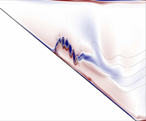
Under certain conditions, as the bolus propagates up-slope, billows resulting from Kelvin–Helmholtz instabilities form along the upper surface (figure 8j). The Richardson number,  $Ri$, is a useful indicator of whether shear instability can (but not necessarily will) occur. It is given as the ratio of stabilising buoyancy and destabilising shear, namely, $Ri = N^2 / (\textrm {d}u/\textrm {d}z)^2$ , where $N^2 = -({g}/{\rho _0})({\textrm {d} \rho }/{\textrm {d}z})$. The case $Ri < 1/4$ can be shown to be a critical value, below which shear instabilities can form and grow (Miles Reference Miles1961). Note, however, that the presence of regions in which the value of $Ri$ is less than this critical value does not indicate that instabilities will definitely form, and their formation may depend on additional criteria (Fructus et al. Reference Fructus, Carr, Grue, Jensen and Davies2009). It was observed that, as wave steepness (and therefore wave-induced velocities) increased, the upper surface of the bolus initially formed approximately perpendicular to the slope, but for waves with increasing incident wave steepness, this upper surface curled around, growing in length along the down-slope direction (figure 9a,c,e). This upper surface was unstable where it formed, and at low wave steepnesses billows formed at the tip only. As the upper surface length grew, the bolus was able to sustain a greater number of billows. Simultaneously, as can be seen in figure 9, the region of the flow for which $Ri < 1/4$ increases, suggesting that shear instability is responsible for these features. The bolus that forms without billows (figure 9a,b) lacks a region where $Ri < 1/4$, whilst the region where $Ri < 1/4$ grows with correspondingly stronger billow formation (figure 9c–f).

Figure 9. Comparison of Richardson number (b,d,f),  $Ri$, in broad tanh profile stratification simulations with increasing $S_w$ for numerical simulations 9L (a,b, $S_w = 0.03$), 9C (c,d, $S_w = 0.12$) and 8R (e,f, $S_w = 0.15$). Panels (a,c,e) show horizontal velocity, $u$ overlaid with isopycnals for the same simulation 5 s later (once any instability has formed). Vertical scale exaggerated for clarity. Corresponding movie of simulation 9C is provided in supplementary movie 7.
The finding that collapsing breaker types cannot be formed in this broad tanh profile stratification can be attributed to the stabilising effect of stratification at the bottom boundary, suppressing shear instabilities that would otherwise produce the global instability characteristic of the collapsing breaker form. Crucially, the density gradient (and therefore the buoyancy frequency term of  $Ri$) at the boundary is increased in this stratification (i.e. $\delta \rho > 0$), acting to increase $Ri$ and stabilise the fluid, and preventing shear instabilities from growing. Bottom shear stress additionally does not experience a considerable peak as the wave shoals for this stratification, as is observed in other wave breaking events (figure 14d). The shear instabilities resemble instabilities described by Xu, Subich & Stastna (Reference Xu, Subich and Stastna2016) for the boluses formed by ISWs of elevation shoaling onto a shelf.
Past studies have identified the stable surging breaker in a similar stratification for both laboratory and numerical experiments (Venayagamoorthy & Fringer Reference Venayagamoorthy and Fringer2007; Arthur et al. Reference Arthur, Koseff and Fringer2017; Allshouse & Swinney Reference Allshouse and Swinney2020; Vieira & Allshouse Reference Vieira and Allshouse2020, e.g.). In those works, as pycnocline thickness increased, bolus transport increased (Allshouse & Swinney Reference Allshouse and Swinney2020; Vieira & Allshouse Reference Vieira and Allshouse2020) and mixing efficiency also increased (Arthur et al. Reference Arthur, Koseff and Fringer2017). For low wave steepnesses, these simulations are in good agreement with those past studies for comparable pycnocline thickness. However, this study systematically shows that, in the parameter space where collapsing and plunging breaker types would be found in the thin tanh profile stratification, the surging breakers in the broad tanh profile stratification become unstable.
4.5.1. Three-dimensional simulations
In this section, 3-D numerical simulations of the surging waves in the broad tanh profile stratification presented in § 4.5 are investigated (figures 10 and 11) to test the validity of the 2-D simulations for a stratification where laboratory data are not available.
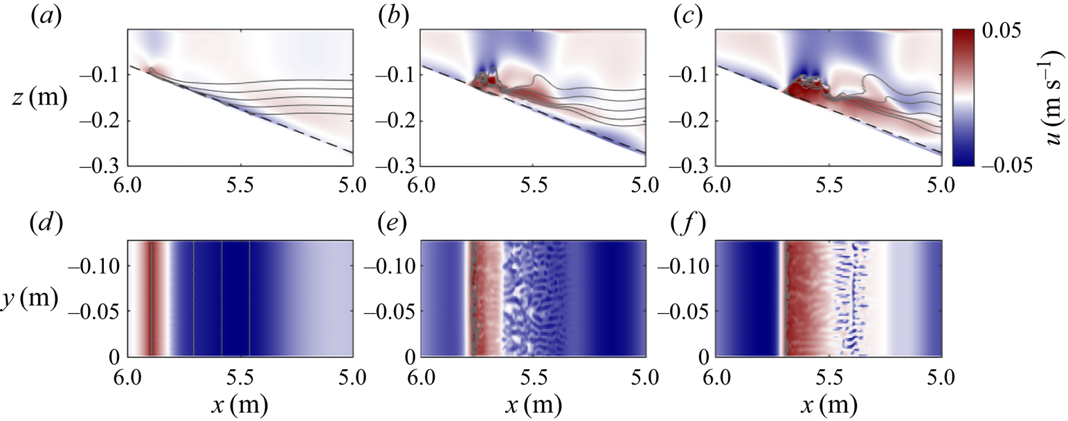
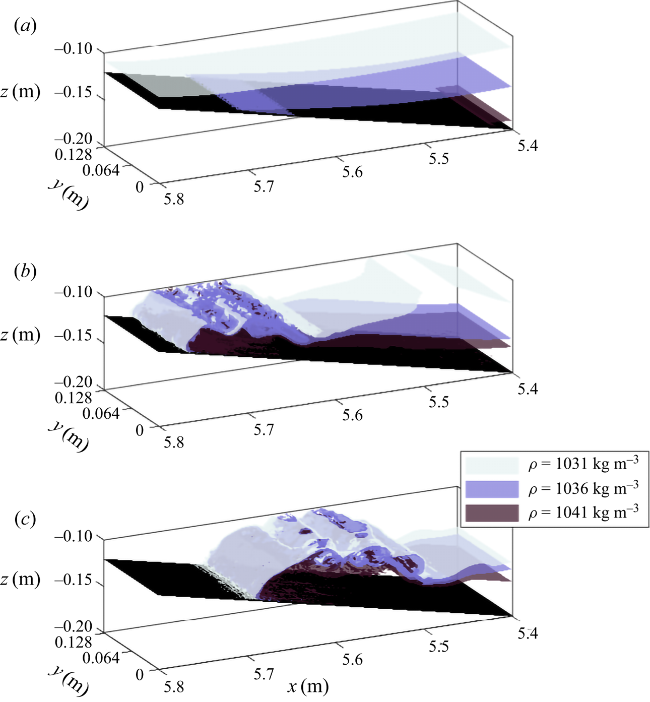
For the lowest incident wave steepness simulation (9L), the dynamics is in line with that seen in the 2-D simulations. Lateral variability only develops after the bolus forms, primarily in the form of small flow features characteristic of lobe-cleft instability at the head of the bolus (figures 10d and 11a). As in the 2-D simulations, as wave steepness increases, further instabilities form, primarily in the form of billows resulting from Kelvin–Helmholtz instabilities on upper surface of the bolus formed (figure 10a–c). As such, the overall flow dynamics is well captured by the previous 2-D simulations, in line with Xu, Stastna & Deepwell (Reference Xu, Stastna and Deepwell2019). However, in the 3-D simulations, the extent of lateral variability of these features increases (figure 11b,c). Not only are these in the form of more prominent features characteristic of lobe-cleft instabilities on the bolus head (figure 10e,f), but with additional transverse features forming as the billows resulting from Kelvin–Helmholtz instabilities are formed (figure 11b,c).
4.6. Fission
In this section, numerical simulation 12L in the surface stratification regime is presented for the wave with wave steepness of  $S_w=0.0871$ in an extended domain propagating over the shallowest slope ( $s=0.03$). This dynamics is in good agreement with fission described in past studies (e.g. Aghsaee et al. Reference Aghsaee, Boegman and Lamb2010; Xu & Stastna Reference Xu and Stastna2020).

Figure 12. Same as figure 5, but for numerical simulation 12L (a–e), representing the fission dynamics in the surface stratification, and numerical simulation 12R (f–j) representing the same wave and dynamics in the broad tanh profile stratification. Time interval between images is  $\Delta t = 10$ s. Vertical scale exaggerated for clarity. Corresponding movies of the simulations are provided in supplementary movies 8 and 9, respectively.
In these numerical simulations, as the wave propagates over the slope the rear face slowly steepens, and the pycnocline at the rear of the wave is displaced upward from its resting level (figure 12a). In the lower layer beneath this upward displacement, the boundary layer flow reversal gradually grows in magnitude and height (figure 12b). This evolves into a bolus at the lower boundary, and an associated wave of elevation forms, which propagates forward through the wave of depression (figure 12b). As the rear of this wave of elevation clears the rear face of the incident wave, a second ISW of elevation forms, which again overtakes the incident wave (figure 12c,d). In these numerical simulations, the BBL dynamics and formation of a bolus are dominant processes in the transition from an ISW of depression to a train of ISWs of elevation, processes not reflected in weakly nonlinear theory (WNL) theory. In the thin tanh profile similar dynamics is observed to the surface stratification case presented, and in this case, this process is repeated so that a train of five small waves of elevation undergo fission and travel up-slope.
The slope of steepness  $s=0.03$ could not be replicated in the laboratory where the slope reached the surface, since doing so would require a $15.5$ m long tank. However, in one laboratory experiment a shoaling ISW propagating over a slope of $s=0.067$, prior to reflection, displayed fission dynamics in the BBL (figure 13) with a train of boundary layer reverse flows forming, each associated with particle resuspension and as a result increased light intensity (figure 13a).

Figure 13. Snapshot of experiment 13L, showing the emergence of fission dynamics in the BBL as the (a) raw experimental image in false colour scheme, and (b) horizontal velocity plot, as in previous figures. Black arrows in (a) indicate the location of the head of each boundary layer vortex. Note that experimental images are made up of images from two cameras merged to form a single image. Corresponding movie of the experiment is provided in supplementary movie 10.
In the broad tanh profile stratification case (figure 12f–j), the wave approaches the slope propagating as a train of periodic waves. As in the thin tanh and surface stratification regimes, slow changes to the KdV terms allow for gradual adjustment of the wave to changing depth (figure 12f,g). Behind the passage of the first depression wave, the same boundary layer feature forms and moves forward in the wave, before breaking ahead as a wave of elevation (figure 12h–j). This wave travels up-slope as a single parcel of fluid, but unlike in the thin tanh profile and surface stratification cases, repeated waves of elevation are not produced (figure 12j), since pursuing waves in the undulating bore disrupt the process.
5. Discussion
5.1. Relevance at the ocean scale
The majority of slopes investigated in this study far exceed typical slopes in the coastal ocean ( $s\approx 0.001$) and lakes ( $s\approx 0.01$). However, the shallower slopes here fall within the margin for average continental slopes ( $s=0.03-0.07$) (Cacchione, Pratson & Ogston Reference Cacchione, Pratson and Ogston2002). Consistent with past studies at the laboratory scale (Aghsaee et al. Reference Aghsaee, Boegman and Lamb2010; Nakayama et al. Reference Nakayama, Sato, Shimizu and Boegman2019; Xu & Stastna Reference Xu and Stastna2020), all waves propagating over these realistic slopes form fission breakers. This process of ISWs of depression evolving into a train of ISWs of elevation has been widely observed in the field (e.g. Orr & Mignerey Reference Orr and Mignerey2003; Shroyer et al. Reference Shroyer, Moum and Nash2009; St Laurent et al. Reference St Laurent, Simmons, Tang and Wang2011) in conditions resembling the thin tanh profile and surface stratification cases investigated here. This process was responsible for inducing dissipation 1–2 orders of magnitude higher than background levels (St Laurent et al. Reference St Laurent, Simmons, Tang and Wang2011).
Due to scaling differences, it is difficult to compare rates of dissipation and mixing in relation to the field. Instead, here, the rates of mixing and dissipation and bottom stress are compared between breaker types in figure 14, to identify which waves are expected to induce the greatest amount of mixing and dissipation, and to make inferences about sediment re-suspension. Estimates of energy conversions calculated by SPINS (Deepwell Reference Deepwell2018) (based on the sorting algorithm of Winters et al. Reference Winters, Lombard, Riley and D'Asaro1995) were processed using Matlab code publicly available at https://github.com/ddeepwel/SPINSmatlab.

Figure 14. Time series of energy dissipated, energy used for mixing and maximum bed stress in positive and negative directions ( $+ t_x$ and $-t_x$, respectively, for each of the numeric simulations 5L (surging), 7L (collapsing), 8L (plunging), 8R (broad tanh profile stratification surging with instability) and 12L (fission) respectively. Data normalised by initial total available energy for energy dissipated and energy to mixing, and by average bed stress over $t = 10 - 20$ s (representing the fully formed wave propagating over the flat bed). Blue crosses represent the times at which frames were plotted in the respective figures.
Energy converted through mixing into background potential energy is given as
 \begin{equation} \phi_m = \phi_d - \phi_i, \end{equation}
where  $\phi _d$ is the rate of change of background potential energy, and $\phi _i$ the rate of conversion from internal energy to potential energy through diffusion. For comparison between simulations with varying initial energetic configurations, mixing and dissipation are presented as percentages of the initial available energy.
The viscous force on the bottom boundary due to fluid motion is  $\boldsymbol {t} = \tau _{ij} n_j$, and the along-bottom (shear) component of that force the dot product with the unit tangent vector
 \begin{equation} t_x = \boldsymbol{t} \boldsymbol{\cdot}(\hat{s}_x,\hat{s}_y). \end{equation}
From this, bed shear stress can be calculated as
 \begin{equation} t_x = \dfrac{\nu \rho_0}{1+h'(x)^2} \left[ 2h'(x)\left(\frac{\partial w}{\partial z} - \frac{\partial u}{\partial x}\right) + (1-h'(x)^2)\left(\frac{\partial u}{\partial z} - \frac{\partial w}{\partial x}\right) \right], \end{equation}
where  $h'$ is the derivative of the bottom depth, $h$.
$h$.
As a general picture, wave energy is dissipated at a low, constant rate on approach to the slope, indicating the waves are stable on approach. As waves reach the slope, and begin to break, the rate of dissipation increases, before gradually levelling off again to a lower rate than on approach. There is very little mixing prior to the onset of breaking, again indicating the wave is stable on approach in most cases, and even after breaking, most energy converted goes to dissipation, rather than to mixing. In the surface stratification regime, the surging and fission breakers upon reaching the slope and breaking do not dissipate energy at a considerably higher rate than the wave on approach, and very little energy is converted to mixing (figure 14a,e). Occurrence of Taylor–Rayleigh and global instabilities in the plunging and collapsing breaker waves respectively are likely responsible for enhanced rate of dissipation as the wave breaks (figure 14b,c). The breaking of ISWs by plunging is anticipated to be dominated by convective instability, whilst ISW breaking by collapsing is anticipated to be shear dominated. Higher mixing efficiencies are anticipated for flows dominated by convection-driven mixing than shear-driven mixing (Ivey et al. Reference Ivey, Bluteau, Gayen, Jones and Sohail2021), however, overall rates of mixing were much higher for the collapsing wave than the plunging wave, with approximately  $14\,\%$ and $4\,\%$ of initial available energy going to irreversible mixing, respectively (despite comparable dissipation). To what extent the mixing is affected by variation of stratification, rather than by changing breaker type would be an interesting area of future study.
The dissipation profile of the surging breaker in the broad tanh profile stratification is very similar to that seen in the surface stratification system (figure 14d), although the presence of Kelvin–Helmholtz instabilities brings about considerably higher mixing after  $t=90$ s. These results indicate the impact of both stratification and breaker type on the transport of energy and mixing by shoaling ISWs. Waves that dissipate energy more slowly are anticipated to transport energy further up-slope. These results are restricted to the 2-D simulations; investigation of mixing in 3-D simulations is beyond the scope of the current paper. Past studies have indicated wave breaking is qualitatively similar in two and three dimensions during the approach to the slope, breaking event, and beginning of the surge up-slope, with differences forming as lateral variability and instabilities (which form only in 3-D simulations) cause billows on the bolus to break down (Arthur & Fringer Reference Arthur and Fringer2014; Xu et al. Reference Xu, Stastna and Deepwell2019). These 3-D effects typically occur away from the leading wave or bolus, and so, although important to mixing, are unlikely to impact the leading behaviour of the wave (Xu et al. Reference Xu, Stastna and Deepwell2019). The presence of lobe-cleft instabilities, and lateral variability at the site of Kelvin–Helmholtz billow generation in 3-D simulations indicates that the underestimation of dissipation and overestimation of mixing would be strongest at the highest wave steepnesses in the broad tanh profile stratification.
Bed stress indicates the degree of sediment re-suspension brought about by the shoaling wave, compared with that as the wave travels over a flat bed. The bolus formed in the surface stratification surging breaker causes relatively high stress, which is anticipated to be associated with high sediment re-suspension and transport up-slope (figure 14a). This is in stark contrast with that seen in the broad tanh profile case (figure 14d), where wave-induced velocities in general are much smaller, and the increase in bed stress as the wave shoals and bolus forms is negligible. This indicates the key importance of stratification type in understanding shoaling-induced sediment transport, even where the dynamics is qualitatively similar. However, Xu et al. (Reference Xu, Subich and Stastna2016) showed that, in 3-D simulations, the bolus formed by shoaling ISW of elevation produced more bed stress than in 2-D simulations due to the formation of lobe-cleft instabilities. This indicates the need for 3-D simulations to effectively estimate bed stress.
In the real-world ocean, background flow (and in particular background shear) plays an important role in the shoaling process (Rayson et al. Reference Rayson, Jones and Ivey2019; Jones et al. Reference Jones, Ivey, Rayson and Kelly2020). Therefore, there is a need for future investigations into shoaling to incorporate these effects.
6. Conclusion
The combination of laboratory experiments and numerical modelling is used here to investigate how the dynamics of shoaling ISWs is affected by the form of the background stratification in which they propagate, for otherwise identical initial conditions. In the thin tanh profile stratification, our numerical experiments are in good agreement with both past numerical studies (Aghsaee et al. Reference Aghsaee, Boegman and Lamb2010; Nakayama et al. Reference Nakayama, Sato, Shimizu and Boegman2019), and past laboratory studies in similar stratification regimes (Sutherland et al. Reference Sutherland, Barrett and Ivey2013). Within the parameter space previously investigated by Aghsaee et al. (Reference Aghsaee, Boegman and Lamb2010) ( $s = 0.01 - 0.3, S_w = 0.0125 - 0.186$), the shoaling dynamics in a thin tanh profile stratification produced in this study was as anticipated for given $s$ and $S_w$. Although the results of Sutherland et al. (Reference Sutherland, Barrett and Ivey2013) were unable to delineate fission-type breakers (as such waves were not observed in the laboratory experiments), these results also follow the Iribarren number-based classifications of past studies for surging, collapsing and plunging breakers in the thin tanh profile stratification.
Laboratory experiments are an effective means of ensuring the validity of numerical model results, and allow a description of the physical breaking processes, whilst numerical models offer a more complete suite of observations of the dynamics, with the opportunity to investigate density, velocity, vorticity, dissipation and stresses, as well as their derivatives. In this new surface stratification regime, the laboratory experiments are in strong agreement with the results of the numerical experiments. This result, alongside agreement with past studies of shoaling ISWs in the thin tanh profile stratification, gives good confidence in the validity of the numerical model used for this study.
Confidence in the validity of the numerical model for this study allowed its extension further into a new broad tanh profile stratification. The formation of a bolus as a wave in the broad tanh profile stratification is well documented in previous numerical and laboratory studies (e.g. Venayagamoorthy & Fringer Reference Venayagamoorthy and Fringer2007; Allshouse & Swinney Reference Allshouse and Swinney2020; Vieira & Allshouse Reference Vieira and Allshouse2020). Vieira & Allshouse (Reference Vieira and Allshouse2020) studied the formation of coherent boluses as waves in a range of similar broad tanh profile stratification where total pycnocline thickness varied, and the stratification in this study represents an extreme of pycnocline thickness. The bolus observed in the broad tanh profile stratification surging-type breakers correspond in polarity to the vortices described by Vieira & Allshouse (Reference Vieira and Allshouse2020), and are of the same form as described previously (Venayagamoorthy & Fringer Reference Venayagamoorthy and Fringer2007). Here, the formation of Kelvin–Helmholtz instabilities along the upper boundary of these boluses are reported for the first time, features previously described for the boluses formed by shoaling ISWs of elevation (Xu et al. Reference Xu, Subich and Stastna2016). Whilst transverse variability and lobe-cleft instabilities form on these boluses, the leading-order behaviour is broadly the same in 2-D simulations as in 3-D simulations (similar to that previously observed by Xu et al. Reference Xu, Stastna and Deepwell2019). These Kelvin–Helmholtz instabilities induce considerable mixing (figure 14d). In other stratification forms, such steep waves would yield other breaking types (figure 2), and the resulting surging bolus therefore would not form.
As the pycnocline thickness increases, and therefore progressively covers a wider part of the water column (the upper layer and then the BBL), the range of shoaling dynamics the wave can take decreases; convective overturning of the plunging breaker type, and collapsing breaker types which arise due to shear instability at the bottom boundary, are both impeded by stratification stabilising the flow above and below the pycnocline respectively. In the surface stratification, the presence of a density gradient throughout the upper layer inhibits the ability for the wave to plunge forward. Instead, the collapsing breaker type is prevalent across the regimes identified in the thin tanh stratification as plunging and collapsing by Aghsaee et al. (Reference Aghsaee, Boegman and Lamb2010). Meanwhile, in the broad tanh profile stratification, the density gradient at the bed also prevents the occurrence of shear-induced global instability and vortices that are responsible for collapsing dynamics when the lower layer is homogeneous. The up-slope bolus produced in the broad tanh profile stratification, where the wave is steep enough, is found to support Kelvin–Helmholtz instabilities on the upper boundary. This is a new dynamics observed here, and not observed in other stratifications, where bolus formation would be prevented by the faster formation of collapsing or plunging breaker types. Previous studies have identified that as pycnocline thickness increases, so too do bolus size and transport (Allshouse & Swinney Reference Allshouse and Swinney2020; Vieira & Allshouse Reference Vieira and Allshouse2020). The extreme of pycnocline thickness in the broad tanh profile stratification therefore can be anticipated to produce larger boluses than in the thinner pycnocline stratifications, thus enabling the observed instabilities to form.
It should be borne in mind that several previous studies with thin tanh profiles have identified the influence of internal wave Reynolds number in the classification of breaking ISWs on uniform slopes (see Nakayama et al. (Reference Nakayama, Sato, Shimizu and Boegman2019) for a recent summary). For reasons presented earlier, such findings are difficult to compare with the classifications for the broad tanh and surface stratification profiles in the present investigation, primarily because of the different wave speed scales required to formulate the relevant Reynolds number. In the studies here, however, values of the internal wave Reynolds numbers based upon the measured wave speed are relatively small (see table 1) compared with those based upon the (external) long wave speed  $c_0$ in the thin tanh studies summarised by Nakayama et al. (Reference Nakayama, Sato, Shimizu and Boegman2019). It is noted that the wave amplitude $A_w$ appears in both $S_w$ and $Re_w$ and there is insufficient evidence in the data to justify ascribing changes in the behaviour of the shoaling waves to Reynolds number effects. Further investigations of this aspect should be pursued for the broad tanh and surface stratification density configurations studied here (by changing the model viscosity, for example).
The SPINS numerical model has previously been successfully used in conjunction with laboratory experiments, and here is shown to be in good agreement with past studies (both numerical and laboratory) in the thin tanh profile system, and in the new surface stratification, is in good agreement with the laboratory experiments. As previously identified (Xu et al. Reference Xu, Stastna and Deepwell2019), the leading-order behaviour of these waves is well captured by 2-D simulations. These results show the importance of representing the stratification of a system in laboratory-scale experiments and models, whilst at the ocean scale, recognising that the form of the stratification may be key to correctly parameterising breaking dynamics, and the rates of mixing, dissipation and sediment dynamics associated with each breaker type. To most effectively represent the real world, further research should investigate the impacts of complex stratifications, for example the double hyperbolic function (see Rayson et al. (Reference Rayson, Jones and Ivey2019) and Manderson et al. (Reference Manderson, Rayson, Cripps, Girolami, Gosling, Hodkiewicz, Ivey and Jones2019)). Furthermore, it is recognised that the field observations of Jones et al. (Reference Jones, Ivey, Rayson and Kelly2020) suggest that background flow can be important in the character of the breaking and shoaling process, and further modelling studies to investigate such effects would be very valuable.
Supplementary material and movies
Supplementary material and movies are available at https://doi.org/10.1017/jfm.2021.1049.
Acknowledgements
Y. Whitchelo is thanked for carrying out preliminary experiments at the University of Dundee as part of her undergraduate studies at the University of St Andrews. Technical assistance in the Novak Laboratory at Newcastle University was provided by D. Dick, S. Patterson and P. Watson and is gratefully acknowledged. This research made use of the Rocket High Performance Computing service at Newcastle University. Professor J. Grue is thanked for useful discussions on this topic at the 4th Norway-Scotland Waves Symposium, which inspired this study. Three anonymous reviewers are thanked for contributions to this manuscript.
Funding
This work was supported by the Natural Environment Research Council (NERC) funded ONE Planet Doctoral Training Partnership (S.H.E., grant number [NE/S007512/1]).
Declaration of interests
The authors report no conflict of interest.
Data availability statement
The data that support the findings of this study are openly available at https://doi.org/10.25405/data.ncl.c.5619616.
Author contributions
S.H.E. performed and analysed the numerical simulations and experiments, wrote the original draft and was responsible for visualisation. M.C. supervised the project, and was responsible for the experimental methodology, resource provision and funding acquisition. M.S. was responsible for the DJL and WNL simulations/calculations, and for providing the numerical model (SPINS). All authors contributed to study conceptualisation and design, and reviewed and edited the manuscript.
Appendix A. Weakly nonlinear theory
While the focus of this manuscript is on large waves for which perturbation theoretic approaches may not give quantitatively accurate information (Lamb & Yan Reference Lamb and Yan1996), we provide a brief summary of KdV theory for the context of the shoaling behaviour. This theory has been used for a variety of purposes in the literature, most pertinently to classify shoaling (Nakayama et al. Reference Nakayama, Sato, Shimizu and Boegman2019). A discussion of the validity of the KdV approach for the large amplitude ISWs of interest here can be found in Grue et al. (Reference Grue, Jensen, Rusås and Sveen1999).
The KdV theory expands the equations in terms of two small parameters, the wave amplitude (or nonlinear parameter) and aspect ratio (or dispersion parameter). The structure of the perturbation velocity and buoyancy fields is assumed to be separable, with the vertical structure,  $\phi (z)$, determined by the solution of a linear eigenvalue problem
 \begin{equation} \phi_{zz} + \frac{N^2(z)}{c_0^2} \phi=0, \end{equation}
where  $\phi (0)=\phi (H)=0$. Here, $c_0$ is the linear, long wave phase speed for each mode, and in this study focus is on mode-1 waves, or those waves with the largest value of $c_0$ for a given stratification.
The temporal and horizontal structure,  $B(x,t)$, of the velocity field is governed by the KdV equation
 \begin{equation} B_t={-}c_0B_x+\alpha B B_x + \beta B_{xxx}, \end{equation}
where subscripts denote partial derivatives, and the nonlinearity,  $\alpha$, and dispersion, $\beta$, parameters are determined from the eigenvalue problem via integration (Lamb & Yan Reference Lamb and Yan1996; Helfrich & Melville Reference Helfrich and Melville2006). Assuming the stratification is fixed, as waves shoal they effectively move into an environment with different relative strengths of the nonlinear and dispersive terms in the KdV equation. Figure 15 shows the linear long wave speed, the nonlinearity and dispersion parameters for the three stratifications used in this study. The depths shown range from the total depth away from the slope to a $50\,\%$ reduction of the total depth. It can be seen that the nonlinearity parameter experiences the largest changes, followed by the propagation speed, with relatively smaller changes in the dispersion parameter. In particular, the nonlinearity parameter is zero away from the slope for the broad stratification. This means that solitary waves cannot be computed from KdV theory, and indeed this is confirmed by the exact DJL theory (not shown). As waves shoal, WNL predicts that they slow down and the dispersion parameter decreases for all three stratifications. However, the change in the nonlinearity parameter suggests that the broad stratification will yield qualitatively different behaviour than the two others, and the $\alpha < 0$ condition indicates that upon shoaling the wave will immediately begin transitioning to a wave of elevation. The exact manifestation of this difference will only become evident through time-dependent numerical simulations.

Figure 15. The coefficients of KdV theory for the three stratifications discussed for simulations as a function of total depth: (a) the linear long wave speed  $c_0$, (b) the nonlinearity coefficient $\alpha$, and (c) the dispersion coefficient $\beta$.


 Open access