


1. Introduction
Models arising in fluid dynamics are often based on the Euler equations and are generally difficult to analyse both at the mathematical and numerical level. As a consequence, the derivation of simplified models is important. But despite this, the design of efficient/validated numerical schemes for such models remains complex, even for the simplified model. The presence of the free surface coupled with the nonlinearities complicates the numerical analysis of such models. Even if some discrete stability properties can be proved (consistency, invariant domains…), some of them, e.g. discrete entropy inequalities, are hardly accessible and in most cases the proof of the convergence of the numerical scheme is out of reach.
A possible approach to validate numerical codes is to compare the results of these codes in configurations for which it is possible to describe the solution exactly using the usual functions. Such solutions are named analytical solutions. In the literature, some examples of analytical solutions for the equations studied here are proposed. One of the most famous concerns a shallow water flow over a parabolic bed (Thacker Reference Thacker1981). An extension of this solution has been proposed by Matskevich & Chubarov (Reference Matskevich and Chubarov2019) and we present here two other extensions. MacDonald et al. (Reference MacDonald, Baines, Nichols and Samuels1995a,Reference MacDonald, Baines, Nichols and Samuelsb) describe a family of analytical solutions with bottom friction, hydraulic jumps and various open-channel cross-sections. Other series of solutions for hydrostatic free surface Euler equations are proposed by Boulanger, Bristeau & Sainte-Marie (Reference Boulanger, Bristeau and Sainte-Marie2013) and references therein.
This paper proposes a new series of analytical solutions that allow us to validate the efficiency of the numerical tools developed for the approximation of the incompressible Euler system with a free surface. These analytical solutions can be adapted to two-dimensional shallow water type models or to models where the velocity is distributed along the vertical direction. Some of the proposed solutions include
(i) wet/dry interfaces;
(ii) the hydrostatic assumption;
(iii) a variable density (the density depends on a tracer concentration).
Figure 1 presents a simplified distribution of the proposed analytical solutions and the corresponding model. The indications Bowl, Hyperbolic or Tank refer to the shape of the basin and  $\S$ precedes the section number to be referred to.

Figure 1. Links between the analytical solutions proposed and the models considered. With indication of the shape of the domain (Bowl, Tank, Hyperbolic) and the section where they are presented.
To validate the numerical implementation of the boundary conditions, we have analytical solutions in a cubic tank with open boundaries and in a semi-open domain with a hyperbolic topography and open boundary. In such cases we have access to the value of all variables and, if necessary, all derivatives of these variables at the boundary.
It is important to notice that these analytical solutions correspond to possible physical configurations, even if they are expressed over simple geometrical domains. To compare them to a laboratory experience or a numerical simulation, it is necessary to be able to impose suitable boundary conditions, which is practicable without difficulties in a numerical simulation but can become more complex in a laboratory experiment.
All the graphics presented is this document represent the exact analytical solutions, but we are able to obtain a good approximation of them by using the Freshkiss3D simulation code (Freshkiss3d 2017) by imposing only the geometry of the domain and the corresponding initial and boundary conditions. With these analytical solutions, it is possible to test simulation codes and to obtain convergence curves when increasing the numerical scheme order and the mesh resolution, see for example Allgeyer et al. (Reference Allgeyer, Bristeau, Froger, Hamouda, Jauzein, Mangeney, Sainte-Marie, Souillé and Vallée2019).
This paper is organized as follows. In § 2 we present the notations and the various forms of the Euler systems used in this paper. In § 3 we propose two extensions of the solution proposed by Thacker (Reference Thacker1981) in a parabolic bowl in the case of the hydrostatic Euler model. Firstly, an extension of the analytical solution with a curved surface in order to have a velocity distributed along the vertical direction. Secondly, an extension of the analytical solution with a planar surface including variable density. In § 4, we consider a domain with a hyperbolic topography for which we can exhibit some solutions for the hydrostatic and the non-hydrostatic Euler model. In § 5, we present a cubic tank domain that permits us to test the boundary conditions for the hydrostatic and the non-hydrostatic Euler model.
2. The Euler system
2.1. Free surface Euler model
Let us first describe below the mass and momentum equations with associated boundary conditions for which we will propose analytical solutions. We assume in this part that the density is constant. We consider the three-dimensional Euler system describing a free surface gravitational flow moving over a bottom topography  $z_b(x,y)$ (unit: m) with constant density
 \begin{gather} \boldsymbol{\nabla} \boldsymbol{\cdot} {\boldsymbol{U}} = 0, \end{gather}
 \begin{gather}\frac{\partial {\boldsymbol{U}}}{ \partial t} + \boldsymbol{\nabla} \boldsymbol{\cdot} ( {\boldsymbol{U}}\otimes {\boldsymbol{U}}) +\frac{1}{\rho_0} \boldsymbol{\nabla} p = \boldsymbol{g} , \end{gather}
where  ${\boldsymbol {U}}(t,x,y,z)=(u,v,w)^\textrm {T}$ is the velocity (unit: $\textrm {m}\ \textrm {s}^{-1}$), $p$ is the fluid pressure (unit: Pa), $\rho _0$ is the density (unit: $\textrm {kg}\ \textrm {m}^{-3}$) assumed to be constant and ${\boldsymbol {g}}= ( 0,0,-g)^\textrm {T}$ represents the gravity force (unit: $\textrm {m}\ \textrm {s}^{-2}$) (where XT is the transpose of X). The quantity nabla denotes $\boldsymbol {\nabla } = ({\partial }/{\partial x}, {\partial }/{\partial y}, {\partial }/{\partial z})^\textrm {T}$. We consider a free surface flow (see figure 2), therefore we assume
 \begin{equation} z_b(x,y)\leqslant z\leqslant \eta(t,x,y) := h(t,x,y)+z_b(x,y), \end{equation}
with  $h(t,x,y)$ the water depth (unit: m) and $\eta(t, x, y)$ the free surface elevation (unit: m).

Figure 2. Flow domain with water height  $h(t,x,y)$, free surface $\eta (t,x,y)$ and bottom $z_b(x,y)$.
2.2. Boundary conditions
At the free surface, the kinematic boundary condition is
 \begin{equation} \frac{\partial \eta}{\partial t} + u_s \frac{\partial \eta}{\partial x} + v_s \frac{\partial \eta}{\partial y} -w_s = 0, \end{equation}
whereas at the bottom we have the no-penetration condition
 \begin{equation} u_b \frac{\partial z_b}{\partial x} + v_b \frac{\partial z_b}{\partial y} -w_b = 0, \end{equation}
where  $U_s=(u_s,v_s,w_s)^\textrm {T}=(u(t,x,y,\eta ),v(t,x,y,\eta ),w(t,x,y,\eta ))^\textrm {T}$, $U_b= (u_b,v_b,w_b)^\textrm {T} =(u(t,x,y,z_b),v(t,x,y,z_b),w(t,x,y,z_b))^\textrm {T}$ with $\eta =\eta (t,x,y)$, $z_b=z_b(x,y)$.
The dynamic boundary condition at the free surface is given by
 \begin{equation} p_s=p(t,x,y,\eta) = p^a(t,x,y). \end{equation}
where  $p_s$ represents the pressure at the free surface and $p^a$ is the atmospheric pressure.
The system (2.1)–(2.6) has to be completed with initial and boundary conditions at the lateral boundaries (inflow, outflow or wall type) that are not detailed here but will be defined for each analytical solution.
2.3. Hydrostatic models
Hydrostatic models consist of neglecting the vertical acceleration of the fluid i.e.
 \begin{equation} \frac{\partial {w}}{\partial {t}} + u\frac{\partial {w}}{\partial {x}} + v\frac{\partial {w}}{\partial {y}} + w\frac{\partial {w}}{\partial {z}} \approx 0. \end{equation}
Hence, the hydrostatic Euler system writes
 \begin{gather} \boldsymbol{\nabla}\boldsymbol{\cdot} {\boldsymbol{U}} = 0, \end{gather}
 \begin{gather}\frac{\partial {\boldsymbol{u}}}{ \partial t} + \boldsymbol{\nabla}_{x,y} \boldsymbol{\cdot} ({\boldsymbol{u}}\otimes {\boldsymbol{u}}) + \frac{\partial ({\boldsymbol{u}} w)}{\partial z} + \frac{1}{\rho_0} \boldsymbol{\nabla}_{x,y} p = 0 , \end{gather}
 \begin{gather}\frac{\partial p}{\partial z} ={-} \rho_0 g, \end{gather}
where  $\boldsymbol {u}(t,x,y,z) = (u,v)^\textrm {T}$ is the horizontal velocity, $\boldsymbol {\nabla }_{x,y}$ corresponds to the projection of $\boldsymbol {\nabla }$ on the horizontal plane, i.e. $\boldsymbol {\nabla }_{x,y} = ({\partial }/{\partial x},{\partial }/{\partial y} )^\textrm {T}$. These equations are completed with the boundary conditions (2.4), (2.5) and (2.6). The vertical momentum equation leads then to the hydrostatic pressure
 \begin{equation} p(t,x,y,z) = p^a(t,x,y) + \rho_0 g (\eta -z). \end{equation}
These hydrostatic models are very often used for the study of geophysical flows, see Brenier (Reference Brenier1999) and Grenier (Reference Grenier1999), such as landslides, glaciers or tsunamis (e.g. Fernandez-Nieto et al. Reference Fernandez-Nieto, Garres-Diaz, Mangeney and Narbona-Reina2016; Allgeyer et al. Reference Allgeyer, Bristeau, Froger, Hamouda, Jauzein, Mangeney, Sainte-Marie, Souillé and Vallée2019) for justifications of such models.
2.4. Passive tracer or variable density
We can consider that the fluid contains a passive tracer  $\phi (t,x,y,z)$ governed by a transport equation
 \begin{equation} \frac{\partial \phi}{\partial t} +\boldsymbol{U}\boldsymbol{\cdot}\boldsymbol{\nabla} \phi = 0. \end{equation}
Equation (2.12) with  $\rho =\rho _0$ implies that this tracer has no impact on the flow.
But we can also consider a fluid where the density is a function of the tracer concentration  $\phi$ i.e. $\rho =\rho (\phi )$ (typically, $\phi$ can represent the temperature or the salinity of the fluid). The function $\rho(\phi)$ being given, the hydrostatic Euler system with variable density writes
 \begin{gather} \boldsymbol{\nabla}\boldsymbol{\cdot} {\boldsymbol{U}} = 0, \end{gather}
 \begin{gather}\frac{\partial \rho}{\partial t} + \boldsymbol{\nabla}\boldsymbol{\cdot} (\rho{\boldsymbol{U}}) = 0, \end{gather}
 \begin{gather}\frac{\partial (\rho \boldsymbol{u})}{ \partial t} + \boldsymbol{\nabla}_{x,y} \boldsymbol{\cdot} (\rho \boldsymbol{u}\otimes {\boldsymbol{U}}) + \boldsymbol{\nabla}_{x,y} p = 0, \end{gather}
 \begin{gather}\frac{\partial p}{\partial z} ={-} \rho g. \end{gather}
The system (2.13)–(2.15) is completed with the boundary conditions (2.4), (2.5), (2.6).
Notice that (2.13) and (2.14) with  $\rho =\rho (\phi )$ give (2.12). But through the density variations in (2.15) and (2.16) the variations of the tracer concentration $\phi (t,x,y,z)$ modify the flow.
3. Parabolic bowl
This first set of analytical solutions we propose are extensions of the solutions introduced by Thacker (Reference Thacker1981). The solution initially proposed by Thacker corresponds to the solution of shallow water equations i.e. a hydrostatic flow where the horizontal velocity ( $u, v$) does not depend on the vertical coordinate $z$. Thacker's approach requires a parabolic shape of the basin and its solution implies treating wet/dry interfaces. We propose here two extensions of Thacker's solutions, the first one having a velocity distributed along the vertical axis, and the second one dealing with a variable density flow. For both of them, the bottom topography is given by
 \begin{equation} z_b(x,y)=\alpha\frac{r^2}{2}, \end{equation}
with  $\alpha >0$ and $r=\sqrt {x^2+y^2}$.
3.1. Hydrostatic Euler model and parabolic topography
We propose here an extension of Thacker's solutions with a curved surface Thacker (Reference Thacker1981) where components of the velocity are functions of the  $z$ variable. The following proposition gives an analytical solution for the hydrostatic Euler model presented in § 2.3:
Proposition 3.1 For some  $t_0\in \mathbb {R}$, $(\alpha ,\beta ,\gamma )\in \mathbb {R}_{+*}^3$, such that $\gamma < 1$ let us consider the functions $h,u,v,w,p$ defined for $t\geqslant t_0$ by
 \begin{gather} h(t,x, y) = \max \left\lbrace 0,\frac{1}{r^2}f\left(\frac{r^2}{\gamma \cos(\omega t)-1}\right) \right\rbrace, \end{gather}
 \begin{gather}u(t,x,y,z) =x \left( \beta \left(z-z_b-\frac{h}{2}\right)+\frac{ \omega \gamma \sin(\omega t)}{2(1-\gamma \cos(\omega t))} \right), \end{gather}
 \begin{gather}v(t,x,y,z) = y\left( \beta \left(z-z_b-\frac{h}{2}\right)+\frac{\omega \gamma \sin(\omega t)}{2(1- \gamma \cos(\omega t))} \right), \end{gather}
 \begin{gather} w(t,x,y,z) ={-}\beta (z-z_b)^2 + \left( \beta h - 2 \varGamma - \beta \alpha r^2 + \frac{\beta}{2} \left( x \frac{\partial h}{\partial x} + y \frac{\partial h}{\partial y} \right) \right)(z-z_b)\nonumber\\ \hspace{-11.6pc}-\frac{\alpha r^2}{2} (\beta h - 2 \varGamma), \end{gather}
 \begin{gather} p(t,x,y,z) = g(\eta-z),\end{gather}
with  $\omega =\sqrt {4\alpha g}$, $\varGamma = -{\omega \gamma \sin (\omega t)}/{2\varLambda }$, $\varLambda = \gamma \cos (\omega t)-1$ and the function $f$ given by
 \begin{equation} f(z)={-}\frac{4g}{\beta^2}+\frac{2}{\beta^2}\sqrt{4g^2+c z+\beta^2 \alpha g (\gamma^2-1)z^2}, \end{equation} $c$ being a non-positive constant.
Then  $h$,
$h$,  $u$,
$u$,  $v$,
$v$,  $w$ and $p$ as defined previously satisfy the three-dimensional hydrostatic Euler system (2.8) and (2.9) completed with the boundary conditions (2.4), (2.5) and (2.6) with $p^a=cst$.
Note that, in (3.2), the maximum is computed at  $(t,x,y,z)$, given to ensure the positivity of the water depth.
Proof. The construction of this solution is inspired by Thacker's work (Thacker Reference Thacker1981). In order to extend the Thacker solution, we first observe that
 \begin{equation} \int_{z_b}^{z_b+h} \varphi(t,x,y) \left(z-z_b - \frac{h}{2}\right) \textrm{d}z = 0, \end{equation}
for all function  $\varphi (t,x,y)$. Thus, if we add a term having the form
 \begin{equation} \varphi(t,x,y) \left(z-z_b - \frac{h}{2}\right), \end{equation}
to the components of the horizontal velocity field, this does not modify a large number of the properties such as the mass conservation. However, some adjustments are necessary to meet all the requirements imposed by (2.1) and (2.2) and allowing us to define the expression of  $\varphi (t,x,y)$. Asymptotically, when $\beta$ goes to zero, the proposed analytical solution converges to the one proposed by Thacker.
The proof of Proposition 3.1 is based on the verification that the proposed expressions for  $h,u,v,w$ and $p$ are solutions of the equations
 \begin{gather} \frac{\partial h}{\partial t}+ \frac{\partial}{\partial x} \int_{z_b}^{z_b+h} u\,\textrm{d} z+ \frac{\partial}{\partial y} \int_{z_b}^{z_b+h} v \,\textrm{d} z=0, \end{gather}
 \begin{gather}\frac{\partial u}{\partial t}+u \frac{\partial u}{\partial x}+v\frac{\partial u}{\partial y}+w\frac{\partial u}{\partial z}+ g \frac{\partial (h+z_b)}{\partial x}=0, \end{gather}
 \begin{gather}\frac{\partial v}{\partial t}+u \frac{\partial v}{\partial x}+v\frac{\partial v}{\partial y}+w\frac{\partial v}{\partial z}+ g \frac{\partial (h+z_b)}{\partial x}=0, \end{gather}
where (3.10) comes from an integration over the vertical axis of the divergence free condition coupled with the two kinematic boundary conditions (2.4) and (2.5).
The details of the computation are given only for (3.10). A more complete computation will be carried out for the two-dimensional case in the proof of Corollary 3.2.
From (3.2) and the definition of  $f(z)$ given in (3.7), we can verify that, on the set where $h(t,x,y)>0$, we have
 \begin{equation} \frac{\partial h}{\partial t} = \frac{\gamma \omega \sin(\omega t)}{(\gamma \cos(\omega t)-1)^2}f'(), \end{equation}
with the notation  $f() =f({r^2}/({\gamma \cos (\omega t)-1}))$. From (3.4), we obtain
 \begin{equation} \int_{z_b}^{z_b+h} u\,\textrm{d}z =\frac{hx\omega \gamma \sin(\omega t)}{2(1-\gamma \cos(\omega t))} , \quad \int_{z_b}^{z_b+h} v \,\textrm{d}z =\frac{hy\omega \gamma \sin(\omega t)}{2(1-\gamma \cos(\omega t))}. \end{equation}
Since
 \begin{equation} \frac{\partial h}{\partial x} ={-} \frac{2 x f()}{r^4}+ \frac{2 x f'()}{r^2 (\gamma \cos(\omega t) - 1))}, \end{equation}
we have
 \begin{equation} \frac{\partial}{\partial x} \int_{z_b}^{z_b+h} u \, \textrm{d} z =\frac{\omega \gamma \sin(\omega t)}{2(1-\gamma \cos (\omega t))}\left[ \frac{f()}{r^2} -\frac{2 x^2 f()}{r^4}+\frac{2 x^2 f'()}{r^2}\right], \end{equation}
and
 \begin{equation} \frac{\partial}{\partial y} \int_{z_b}^{z_b+h} v \, \textrm{d} z =\frac{\omega \gamma \sin(\omega t)}{2(1-\gamma \cos (\omega t))}\left[ \frac{f()}{r^2} -\frac{2 y^2 f()}{r^4}+\frac{2 y^2 f'()}{r^2}\right]. \end{equation}
We deduce that
 \begin{equation} \frac{\partial}{\partial x} \int_{z_b}^{z_b+h} u \, \textrm{d} z+ \frac{\partial}{\partial y} \int_{z_b}^{z_b+h} v\, \textrm{d} z = \frac{\omega \gamma \sin(\omega t)}{(1-\gamma \cos (\omega t))^2} f'(), \end{equation}
and (3.10) is satisfied.
In figure 3, the shape of the free surface of the analytical solution is plotted at different time instants. In Allgeyer et al. (Reference Allgeyer, Bristeau, Froger, Hamouda, Jauzein, Mangeney, Sainte-Marie, Souillé and Vallée2019), convergence curves towards the analytical solution are obtained with the numerical code Freshkiss3d (2017).

Figure 3. Analytic solution for three-dimensional axisymmetric parabolic bowl (see Proposition 3.1): free surface at  $t=0$ (red), $t=T/4$ (dark grey), $t=T/2$ (blue), with the period $T$ defined by $T=2 {\rm \pi}/\omega$ and for parameters set to $h_0=1\ \textrm {m}$, $\alpha =2\ \textrm {m}^{-1}$, $\beta =1\ \textrm {m}^{-1}\ \textrm {s}^{-1}$, $\gamma =0.3$, $c=-1\ \textrm {s}^{-4}$, $L=1$ m.
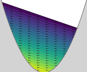
In figure 4, we present an axial section of the analytical solution at four time instants ( $t=0, T/6, T/3, T/2$) for parameter set $h_0=1\ \textrm {m}$, $\alpha = 2 \ \textrm {m}^{-1}$, $\beta = 1 \ \textrm {m}^{-1}\ \textrm {s}^{-1}$, $\gamma =0.3$, $c=-1 \ \textrm {s}^{-4}$, $L=1\ \textrm {m}$. The arrows represent the velocity field and the colour shading gives the velocity norm.

Figure 4. Analytic solution for three-dimensional axisymmetric parabolic bowl (see Proposition 3.1): velocity field and norm at  $t=0 , T/6, 2T/6, T/2$, in $(x,y=0,z)$ slice plane with the period $T$ defined by $T=2 {\rm \pi}/\omega$ and for parameters set to $h_0=1$ m, $\alpha =2\ \textrm {m}^{-1}$, $\beta =1 \ \textrm {m}^{-1}\ \textrm {s}^{-1}$, $\gamma =0.3$, $c=-1 \ \textrm {s}^{-4}$, $L=1$ m.
The analytical solution proposed in Proposition 3.1 can be also expressed in a two-dimensional  $(x,z)$-domain and the following corollary holds:
Corollary 3.2 The analytical solution depicted in Proposition 3.1 can be written in the two-dimensional case. With obvious notations and  $\beta >0$, we choose $\gamma \leqslant 2g/(\beta \omega )$, $c>0$, and we consider the functions $h,u,w,p$ defined for $t\geqslant t_0$ by
 \begin{gather} h(t,x) = \max \left\lbrace 0,f\left(x-\frac{\gamma}{\omega} \sin(\omega t) \right) \right\rbrace, \end{gather}
 \begin{gather}u(t,x,z) = \beta \left( z-z_b-\frac{h}{2}\right)+\gamma \cos(\omega t) , \end{gather}
 \begin{gather}w(t,x,z) = \alpha \beta x z - \frac{\alpha^2 \beta}{2} x^3 - \frac{\alpha \beta}{2} x h(t,x) + \frac{\beta}{2} \left(z-\frac{\alpha }{2}x^2\right) \frac{\partial h}{\partial x} +\alpha \gamma x \cos(\omega t), \end{gather}
 \begin{gather}p(t,x,z) = g(\eta-z), \end{gather}
with  $\omega =\sqrt {\alpha g}$, a bottom topography defined by
 \begin{equation} z_b(x)=\frac{\alpha}{2} x^2, \end{equation}
and a function  $f$ given by
 \begin{equation} f(z) ={-}\frac{4 g}{\beta^2} + \frac{2}{\beta^2}\sqrt{4 g^2 + \beta^2c^2 - \beta^2(\omega z + c)^2}. \end{equation}
Then,  $h,u,w,p$ as defined previously satisfy the two-dimensional hydrostatic Euler system completed with the boundary conditions (2.4), (2.5) and (2.6) with $p^a=cst$.
Proof. It is enough to verify that the expressions for  $u$,
$u$,  $w$ and $h$ are solutions of the following equations:
 \begin{gather} \frac{\partial h}{\partial t}+ \frac{\partial}{\partial x} \int_{z_b}^{z_b+h} u(x,z) \,\textrm{d} z=0, \end{gather}
 \begin{gather}\frac{\partial u}{\partial t}+u \frac{\partial u}{\partial x}+w\frac{\partial u}{\partial z}+ g \frac{\partial (h+z_b)}{\partial x}=0, \end{gather}
where  $w$ is then given thanks to the incompressibility condition by
 \begin{equation} w(t,x,z) ={-}\frac{\partial}{\partial x}\int_{z_b}^z u\,\textrm{d}z. \end{equation}
From (3.19) and the definition of  $f(z)$ given in (3.24), we can verify that, on the set where $h(t,x)>0$, we have
 \begin{equation} \frac{\partial h}{\partial t} ={-}\gamma \cos(\omega t) f'\left(x-\frac{\gamma}{\omega} \sin(\omega t) \right). \end{equation}
From (3.20) and using (3.8) we find
 \begin{equation} \int_{z_b}^{z_b+h} u(x,z) \, \textrm{d} z = h \gamma \cos(\omega t). \end{equation}
And since
 \begin{equation} \frac{\partial h}{\partial x} =f'\left(x-\frac{\gamma}{\omega} \sin(\omega t) \right), \end{equation}
Equation (3.25) is satisfied.
In order to verify (3.26), we start from the definition of  $u(t,x,z)$ leading to
 \begin{equation} \frac{\partial u}{\partial t} = \frac{\beta \gamma \cos (\omega t)}{2} f'() -\gamma \omega \sin(\omega t), \end{equation}
and
 \begin{equation} u\frac{\partial u}{\partial x} ={-}\beta \left( 4 \alpha x + \frac{1}{2} f'() \right) \left[\beta \left( z-2\alpha x^2-\frac{1}{2}f()\right)+\gamma \cos(\omega t)\right], \end{equation}
with the notation  $f()= f(x-({\gamma }/{\omega }) \sin \omega t)$. Moreover, we have
 \begin{equation} w\frac{\partial u}{\partial z} = \beta\left(4 \alpha \beta x z - 8 \alpha^2 \beta x^3 - 2\alpha \beta x f() + \beta \left(\frac{z}{2}-\alpha x^2\right) f'()+4\alpha \gamma x \cos(\omega t)\right). \end{equation}
And the pressure term gives
 \begin{equation} g \frac{\partial (h + z_b)}{\partial x} = gf'()+4 g \alpha x. \end{equation}
Summing the last four expressions, all the terms without  $f()$ or $f'()$ are equal to $4 g \alpha x$ whereas the terms containing $f()$ only are equal to zero. The terms containing only $f'()$ are equal to $g-({\beta \gamma }/{2})\cos \omega t$, and the terms containing $f()\cdot f'()$ equal ${\beta ^2}/{4}$. Now, we have to observe that (3.24) gives
 \begin{equation} f'\left(x-\frac{\gamma}{\omega} \sin(\omega t) \right) ={-}\frac{2 \omega(\omega x - \gamma \sin(\omega t))}{\sqrt{4 g^2 - 2 c \beta^2 - \beta^2 (\omega^2 x-2\gamma \omega \sin(\omega t)+ \gamma^2 \sin^2(\omega t))}}. \end{equation}
Since
 \begin{equation} f(\xi)\cdot f'(\xi) ={-}\frac{4 g}{\beta^2} f'()-\frac{4 \omega^2}{\beta^2}\xi, \end{equation}
the expressions for  $h,u$ and $w$ inserted in (3.26) lead to $2 g\alpha x - \omega ^2 x$, and this term vanishes under the condition $\omega =\sqrt {2 g \alpha }$.
3.2. Hydrostatic Euler equation with variable density
The analytical solution proposed here is based on the analytical solution presented by Thacker (Reference Thacker1981) when the free surface remains planar. The initial Thacker solution is valid for the two-dimensional Saint-Venant system and also for the three-dimensional incompressible and hydrostatic Euler system with constant density. The extension proposed in the following proposition gives an analytical solution for the hydrostatic Euler system with variable density (2.13)–(2.15):
Proposition 3.3 For any non-negative function  $\rho : s\mapsto \rho (s)$ and for some $(\alpha ,\eta ,a,h_0)\in \mathbb {R}^2\times \mathbb {R}_+^2$, let us consider the functions $h,u,v,w,p, \phi$ defined for $(x,y)\in [-L/2, L/2]^2$, $t\geqslant t_0$ by
 \begin{equation} \left.\begin{gathered} h(t,x,y) = \max\left\{0,h_0- \alpha \frac{\left(x -\eta\cos(\omega t)\right)^2 + \left(y - \eta\sin(\omega t)\right)^2}{2}\right\}, \\ u(t,x,y,z) ={-}\eta\omega\sin(\omega t),\\ v(t,x,y,z) = \eta\omega\cos(\omega t),\\ w(t,x,y,z) ={-}\alpha\eta\omega\left(x\sin(\omega t) - y\cos(\omega t)\right), \\ p(t,x,y,z) = p^a(t) + \int_z^{h+z_b} \rho (\phi(t,x,y,z_1))\,\textrm{d}z_1,\\ \phi(t,x,y,z) = a \left( h+z_b - z\right), \end{gathered}\right\}\end{equation}
with  $\omega =\sqrt {\alpha g}$. We recall that the topography is given by $z_b(x,y)= ({\alpha }/{2}) r^2$. Then, $h,u,v,w,p$ and $\phi$ as defined previously satisfy the three-dimensional hydrostatic Euler system with variable density (2.13)–(2.15) completed with the kinematic boundary conditions (2.4) and (2.5).
A three dimensional representation of the free surface solution proposed in proposition3.3 is given in figure 5. A plot of the analytical solution (in the plane  $y=0$) at several time instants is given in figure 6, where we can observe that the density isovalue lines remain parallel to the planar surface.

Figure 5. Analytical solution of radially symmetric parabolic bowl with variable density (see Proposition 3.3), three-dimensional planar surface: free surface at  $t=0$ (red), $t=T/4$ (dark grey), $t=T/2$ (blue), with the period $T$ defined by $T=2 {\rm \pi}/\omega$ and for parameters set to $\eta =0.1 \ \textrm {m}$, $h_0=0.1 \ \textrm {m}$, $a=1$, $\alpha =1 \ \textrm {m}^{-1}$, $L=4 \ \textrm {m}$.

Figure 6. Analytical solution of radially symmetric parabolic bowl with variable density (see Proposition 3.3): free surface, velocity vectors and tracer for  $t=0, T/6, 2T/6, T/2$, in $(x,y=0,z)$ slice plane with the period $T$ defined by $T=2 {\rm \pi}/\omega$ and for parameters set to $\eta =0.1 \ \textrm {m}$, $h_0=0.1 \ \textrm {m}$, $a=1$, $\alpha =1 \ \textrm {m}^{-1}$, $L=4 \ \textrm {m}$.
Situations where  ${\partial \rho }/{\partial z} \geqslant 0$ can be encountered in practice (upwellings, Rayleigh–Bénard instabilities,…). The analytical solutions given in Proposition 3.3 exhibit situations where ${\partial \rho }/{\partial z}$ remains non-negative with time; of course such solutions are unstable in the sense that they cannot be reproduced neither by laboratory experiments nor captured at the discrete level.
Proof. Starting from Thacker's solution with constant density (Thacker Reference Thacker1981), we have only to verify that the chosen expression for the density  $\rho (t,x,y,z) = a(\eta (t,x,y)-z)$ does not modify this solution. We have $\partial _z p = - \rho (t,x,y,z) g$ due to the hydrostatic hypothesis. If we note $\eta =\eta (t,x,y) = h(t,x,y)+z_b(x,y)$, $\rho (t,x,y,z) = \phi (\eta (t,x,y)-z)$ and $p(t,x,y,\eta (t,x,y)) = p^a(t)$, for $\phi \in C^1({\mathbb {R}})$ we have
 \begin{align} \boldsymbol{\nabla}_{x,y} p &= g\boldsymbol{\nabla}_{x,y} \int_z^{\eta} \rho(t,x,y,\xi) \,\textrm{d}\xi\nonumber\\ &= g\boldsymbol{\nabla}_{x,y} \int_z^{\eta} \phi(\eta-\xi) \,\textrm{d}\xi\nonumber\\ &=g \int_z^{\eta} \boldsymbol{\nabla}_{x,y} \phi(\eta-\xi) \,\textrm{d}\xi +g\phi(0) \boldsymbol{\nabla}_{x,y} \eta \nonumber\\ &=g \int_z^{\eta} \phi'(\eta-\xi) \boldsymbol{\nabla}_{x,y} \eta \,\textrm{d}\xi +g \phi(0)\boldsymbol{\nabla}_{x,y} \eta \nonumber\\ &=g \boldsymbol{\nabla}_{x,y} \eta \int_{\eta-z}^0 \phi'(s) \,\textrm{d}s +g \phi(0) \boldsymbol{\nabla}_{x,y} \eta \quad \text{with}\ s=\eta -\xi\nonumber\\ &=g \phi(\eta-z) \boldsymbol{\nabla}_{x,y} \eta \nonumber\\ &=g \rho(t,x,y,z) \boldsymbol{\nabla}_{x,y} \eta. \end{align}
If we consider the momentum equation (2.15), using the previous evaluation of the pressure term, we can conclude that  $u$ is the solution of (2.9) that corresponds to the momentum equation with constant density.
But generally, this expression for the density does not verify the conservation equation (2.14)
 \begin{equation} \partial_t \rho + \boldsymbol{\nabla}\boldsymbol{\cdot} (\rho U) =0. \end{equation}
In the proposed analytical solution, since  $u$ and $w$ are independent of $x$ and $z$, then we have
 \begin{align} \partial_t \rho + \boldsymbol{u} \boldsymbol{\cdot} \boldsymbol{\nabla}_{x,y} \rho + w \partial_z \rho &= \phi'(\eta-z) \partial_t \eta + \phi'(\eta-z) \boldsymbol{u}\boldsymbol{\cdot}\boldsymbol{\nabla}_{x,y} \eta - \phi'(\eta-z) w \nonumber\\ &=\phi'(\eta-z) (\partial_t \eta + \boldsymbol{u}\boldsymbol{\cdot}\boldsymbol{\nabla}_{x,y} \eta - w ) =0, \end{align}
since at the free surface the kinematic boundary condition gives  ${\partial _t \eta + \boldsymbol {u}\boldsymbol {\cdot }\boldsymbol {\nabla }_{x,y} \eta - w = 0}$.
The analytical solution depicted in Proposition 3.3 admits a two-dimensional version.
Corollary 3.4 With obvious notations, the functions  $h,u,w,p,\phi$ defined for $t\geqslant t_0$ by
 \begin{equation} \left.\begin{gathered} h(t,x) = \max\left\{0,h_0- \alpha \frac{\left(x -\eta\cos(\omega t)\right)^2 }{2}\right\}, \\ u(t,x,z) ={-}\eta\omega\sin(\omega t),\\ w(t,x,z) ={-}\alpha x \eta\omega \sin(\omega t), \\ p(t,x,z) = p^a(t) + \int_z^{h+z_b} \rho (\phi(t,x,z_1))\,\textrm{d}z_1,\\ \phi(t,x,z) = a \left( \eta - z\right), \end{gathered}\right\}\end{equation}
with a bottom topography defined by  $z_b(x)=\alpha x^2/2$ and with the kinematic boundary conditions (2.4) and (2.5) satisfy the two-dimensional version of the hydrostatic Euler system with variable density (2.13)–(2.16) for any $(a, \alpha , \eta , h_0)\in \mathbb {R}^3 \times \mathbb {R}_+$.
Proof. The proof is the same as for Proposition 3.3 and is not detailed here.
4. Hyperbolic topography
In this section, we are interested in characterizing the shallow water analytical solutions of the Euler system. More precisely, we show that, under a reasonable hypothesis, we can find all the solutions of the Euler free surface equations whose horizontal velocity does not depend on  $z$. More precisely, we exhibit the analytical solutions of the system (2.1) and (2.2) completed with the boundary conditions (2.4), (2.5) and (2.6) having a velocity field of the form $u=\bar {u}(t,x,y)$ and $v= \bar {v}(t,x,y)$. Moreover, it is possible to deduce the shallow water analytical solutions of the hydrostatic Euler equations (2.8) and (2.9). At the numerical level, these solutions give access to analytical solutions of the free surface Euler equations with an open boundary and wet/dry interfaces.
4.1. Non-hydrostatic Euler equations
Proposition 4.1 For some  $( \alpha , \beta , c_0) \in {{\mathbb {R}}^+}^3$, $( b_0, t_0) \in {\mathbb {R}}^2$, $t_1\in \mathbb {R}_+^*$, $\theta \in [0, 2{\rm \pi} ]$, let us consider the functions $h, u, v, w$ and $p$ defined for $t \geqslant t_0$, $(x,y)\in {{\mathbb {R}}^+}^2$ and $z \in [z_b(x,y), \eta (t,x,y)]$ by
 \begin{equation} \left.\begin{gathered} h(t,x,y) = \max\left\{0, \alpha f(t) - b_0 - z_b(x,y)\right\}, \\ u(t,x,y,z) = f(t) (x \cos\theta +y \sin\theta +\beta) \cos\theta, \\ v(t,x,y,z) = f(t) (x \cos\theta +y \sin\theta +\beta) \sin\theta, \\ w(t,x,y,z) ={-}f(t) (z+b_0) ,\\ p(t,x,y,z) = p^{a,0}(t) + f^2(t)(\eta^2-z^2) + \left(2 b_0 f^2(t) + g\right) (\eta-z), \end{gathered}\right\} \end{equation}
where  $f(t)=1/(t-t_0+t_1)$, $p^{a,0}(t)$ is a given function and the topography is defined by
 \begin{equation} z_b(x,y)=\frac{c_0}{x \cos\theta +y \sin\theta+\beta}-b_0. \end{equation}
 Then  $h, u, v$ and $p$ as defined previously satisfy the Euler system (2.1) and (2.2) completed with the boundary conditions (2.4), (2.5) and (2.6).
Remark 4.2 In Proposition 4.1, we have to deal with an open boundary, the associated boundary conditions to impose can be obtained by considering the value of the analytical expressions of the solution on the corresponding domain boundary.
Proof. The proof relies on simple computations that are detailed hereafter. For the sake of simplicity, the computations are carried out in two dimensions  $(x,z)$ corresponding to $\theta = 0$.
Assuming  $u=\bar {u}(t,x)$, the divergence free condition (2.1) coupled with (2.5) gives
 \begin{equation} w ={-}z\frac{\partial \bar{u}}{\partial x} + \frac{\partial (z_b\bar{u})}{\partial x}, \end{equation}
and the two components of (2.2) give
 \begin{gather} \frac{\partial \bar{u}}{\partial t} + \bar{u}\frac{\partial \bar{u}}{\partial x} + \frac{\partial p}{\partial x}=0, \end{gather}
 \begin{gather}-z\left( \frac{\partial^2 \bar{u}}{\partial x\partial t} + \bar{u} \frac{\partial^2 \bar{u}}{\partial x^2} - \left(\frac{\partial \bar{u}}{\partial x}\right)^2\right) + \frac{\partial^2 (z_b\bar{u})}{\partial x\partial t} + \bar{u}\frac{\partial^2 (z_b\bar{u})}{\partial x^2} - \frac{\partial \bar{u}}{\partial x}\frac{\partial (z_b\bar{u})}{\partial x} + \frac{\partial p}{\partial z} ={-}g. \end{gather}
From (4.4), (4.5) and (2.6), we deduce that the pressure  $p$ satisfies
 \begin{equation} p(t,x,\eta)=p^{a,0}(t),\quad\mbox{and}\quad\frac{\partial^2 p}{\partial x\partial z} = \frac{\partial^3 p}{\partial z^3}=0, \end{equation}
therefore, the pressure  $p$ has necessarily the form
 \begin{equation} \bar{p} = p^{a,0}(t) + \frac{a(t)}{2} \left( \eta^2 - z^2 \right) + b(t) \left( \eta - z \right), \end{equation}
where  $a=a(t)$ and $b=b(t)$ are two functions to be determined.
Hence, the shallow water solutions of the incompressible Euler system with a free surface are characterized by
 \begin{gather} \frac{\partial h}{\partial t} + \frac{\partial (h\bar{u})}{\partial x} = 0, \end{gather}
 \begin{gather}\frac{\partial \bar{u}}{\partial t} + \bar{u}\frac{\partial \bar{u}}{\partial x} + \left(a(t)\eta + b(t)\right)\frac{\partial \eta}{\partial x} = 0, \end{gather}
 \begin{gather}\frac{\partial^2 \bar{u}}{\partial x\partial t} + \bar{u}\frac{\partial^2 \bar{u}}{\partial x^2} - \left(\frac{\partial \bar{u}}{\partial x}\right)^2 ={-}a(t), \end{gather}
 \begin{gather}\frac{\partial^2 (z_b\bar{u})}{\partial x\partial t} + \bar{u}\frac{\partial^2 (z_b\bar{u})}{\partial x^2} - \frac{\partial \bar{u}}{\partial x}\frac{\partial (z_b\bar{u})}{\partial x} = b(t)-g. \end{gather}
Now, subtracting from (4.10) the derivative of (4.9) with respect to the variable  $x$ gives
 \begin{equation} 2 \left(\frac{\partial \bar{u}}{\partial x}\right)^2 = a(t) - \frac{\partial}{\partial x}\left(\left(a(t)\eta + b(t)\right)\frac{\partial \eta}{\partial x}\right). \end{equation}
 Likewise, subtracting (4.10) multiplied by  $z_b$ from (4.11) gives
 \begin{equation} \frac{\partial \bar{u}}{\partial t} \frac{\partial z_b}{\partial x} + \bar{u}^2\frac{\partial^2 z_b}{\partial x^2} + \bar{u}\frac{\partial \bar{u}}{\partial x}\frac{\partial z_b}{\partial x} + a(t)z_b = b(t)-g. \end{equation}
The solution  $\eta =\eta (t,x)$ of (4.9) can be obtained explicitly if we assume $a(t)>0$ and then $h(t,x)$ is given by
 \begin{equation} h(t,x) ={-}z_b(x)-\frac{b(t)}{a(t)} + \frac{1}{a(t)}\sqrt{ a(t) \left( F_1(t) - \bar{u}^2 - 2\int^x \partial_t \bar{u} \,\textrm{d}s \right)}, \end{equation}
where  $t\mapsto F_1(t)$ is any function such that $F_1(t)\geqslant \bar {u}^2+2\int ^x \partial _t \bar {u} \,\textrm {d}s$.
A solution of the derivative of (4.10) with respect to the variable  $x$ is given by
 \begin{equation} \bar{u}(t,x)=\frac{u_1(x)}{t-t_0+t_1}. \end{equation}
Let us assume that (4.15) holds true. Inserting (4.15) into (4.8), we can write this equation formally in the form
 \begin{equation} \frac{\partial (h u_1)}{\partial x} + \frac{t-t_0+t_1}{u_1} \frac{\partial (h u_1)}{\partial t}=0, \end{equation}
then we apply the characteristic method following  $t'(x) = ({t-t_0+t_1})/{u_1}$ leading to $t(x) = (t-t_0+t_1) \int ^x ({1}/{u_1(s)})\,\textrm {d}s$ and we can exhibit a formal expression for $h(x,t)$ of the form
 \begin{equation} h(t,x)=\frac{F_0\left( (t-t_0+t_1)\exp\left({-\displaystyle\int^x \dfrac{\textrm{d}s}{u_1(s)}}\right)\right)}{u_1(x)}, \end{equation}
where  $\xi \mapsto F_0(\xi )$ is any function.
Likewise, inserting the expression for  $\bar {u}$ given by (4.15) into (4.14) gives another expression for $h(t,x)$ with
 \begin{align} h(t,x) &={-}z_b(x)-\frac{b(t)}{a(t)}\nonumber\\ &\quad + \frac{1}{a(t)(t-t_0+t_1)}\sqrt{a(t)\left( (t-t_0+t_1)^2 F_1(t) - u_1^2(x) + 2\int^x u_1(s)\,\textrm{d}s \right)}. \end{align}
Now, inserting the expression (4.15) into (4.10) implies that necessarily
 \begin{equation} a(t) = \frac{a_0}{(t-t_0+t_1)^2}, \end{equation}
with  $a_0\in \mathbb {R}$. Similarly, inserting the expression (4.15) into (4.11) allows us to obtain the expression for $b(t)$ of the form
 \begin{equation} b(t) = g+\frac{2 b_0}{(t-t_0+t_1)^2}, \end{equation}
with  $b_0\in \mathbb {R}$.
Thus, (4.18) gives
 \begin{align} h(t,x) &={-}z_b(x)-\frac{b_0}{a_0} - \frac{g}{a_0}(t-t_0+t_1)^2 \nonumber\\ &\quad + \frac{1}{\sqrt{a_0}}\sqrt{(t-t_0+t_1)^2 F_1(t) - u_1^2(x) +2\int^x u_1(s)\,\textrm{d}s}. \end{align}
The two expressions for  $h(t,x)$, namely (4.17) and (4.21), are compatible only if the primitive function associated with ${1}/{u_1(x)}$ is a logarithmic function of $x$, leading to
 \begin{equation} u_1(x) = \gamma x + \beta, \end{equation}
with  $(\beta ,\gamma ) \in \mathbb {R}^2$. Inserting (4.22) into (4.10) gives that
 \begin{equation} \gamma^2+\gamma = a . \end{equation}
Now, from (4.18) we can set  $- u_1^2(x) +2\int ^x u_1(s)\,\textrm {d}s = C$ in order to have $h(t,x)+z_b(x)$ only depending on time $t$ i.e.
 \begin{equation} \frac{\partial \eta}{\partial x} = 0. \end{equation}
This property inserted into (4.9) gives  $\gamma = 1$, and using (4.23), $a_0=2$.
Finally, we have obtained that
 \begin{equation} u_1(x) = x+\beta, \end{equation}
and  $h=z_b(x)+F_\eta (t)$. These two expressions inserted in (4.8) give
 \begin{equation} \left\{\begin{array}{@{}l} z_b(x) = \dfrac{c_0}{x+\beta} - b_0\\ h(t,x) = \dfrac{\alpha}{t-t_0+t_1} - \dfrac{c_0}{x+\beta} \end{array}\right. \end{equation}
These expressions are valid only if  $h(t,x)\geqslant 0$. Thus, the expressions (4.25), (4.26) and (4.15) give a proof of Proposition 4.1 in the two-dimensional ( $x,z$) setting (when $\theta = 0$).
Corollary 4.3 If we assume that all the solutions of (4.10) can be written in the form (4.15), Proposition 4.1 gives all the solutions of the free surface Euler equations in which  $u$ and $v$ do not depend on $z$.
$z$.
Figure 7 shows the velocity field at times  $t=0, 0.05, 0.1$ and $0.15$ seconds for a given set of the parameters values ( $\alpha =0.5 \ \textrm {m}\ \textrm {s}$, $\beta = 0.1\ \textrm {m}$, $b_0=0.4\ \textrm {m}$, $t_0-t_1=2$ s, $c_0=1.2 \ \textrm {m}^{2}$). The solution proposed in Proposition 4.1 is not a solution of the hydrostatic formulation of the equation, but we can easily deduce a hydrostatic analytical solution by reversing the direction of the velocity field. This result is described in the following section.

Figure 7. Analytical solution for hyperbolic topography (see Proposition 4.1): velocity norm and vectors at  $t=0$, 0.05, 0.1 and $0.15$ s in $(x,y=0,z)$ for parameters set to $\alpha =0.5 \ \textrm {m}\ \textrm {s}$, $\beta = 0.1 \ \textrm {m}$, $b_0=0.4 \ \textrm {m}$, $t_0-t_1=2$ s, $c_0=1.2 \ \textrm {m}^{2}$.
4.2. Hydrostatic Euler equations
If we consider the hydrostatic Euler system (2.8) and (2.9), the following result holds:
Proposition 4.4 For some  $( \alpha , \beta , c_0, t_0) \in {{\mathbb {R}}^+}^3$, $(b_0,t_o) \in {\mathbb {R}}^2$, $t_1\in \mathbb {R}_+^*$, $\theta \in [0, 2{\rm \pi} ]$, let us consider the functions $h, u, v, w$ and $p$ defined for $t \geqslant t_0$ by
 \begin{equation} \left.\begin{gathered} h(t,x,y) = \max\{0,\alpha f(t) - b_0 - zb(x,y)\}, \\ u(t,x,y,z) ={-}(x \cos\theta +y \sin\theta +\beta) \cos\theta/f(t), \\ v(t,x,y,z) ={-}(x \cos\theta +y \sin\theta +\beta) \sin\theta/ f(t), \\ w(t,x,y,z) = (b_0+z)/ f(t),\\ p(t,x,y,z) = p^{a,0}(t)+p^{a,1}(t,x,y) + g (\eta-z), \end{gathered}\right\} \end{equation}
where  $f(t)=t-t_0+t_1$, the bottom topography given by $z_b(x,y)={c_0}/(x \cos \theta +y \sin \theta +\beta)-b_0$ and $p^{a,0}(t)$ a given function with also
 \begin{equation} p^{a,1}(t,x,y) ={-}\left((x \cos\theta +y \sin\theta)^2+2 \beta (x \cos\theta +y \sin\theta)\right)/f(t)^2. \end{equation}
Then,  $h, u, v, p$ as defined previously satisfy the hydrostatic Euler system (2.8) and (2.9) completed with the boundary conditions (2.4), (2.5) and (2.6).
Proof. The main idea of the proof is to observe that the analytical solution proposed in Proposition 4.1 satisfies
 \begin{equation} \frac{\partial {w}}{\partial {t}} = u\frac{\partial {w}}{\partial {x}} + v\frac{\partial {w}}{\partial {y}} + w\frac{\partial{w}}{\partial {z}}={-}\frac{b_0+z}{ f(t)^2}. \end{equation}
It is sufficient to reverse the direction of the components of the velocity to cancel the non-hydrostatic part of the third momentum equation. Compared to Proposition 4.1, with opposite values of  $u$ and $v$, the water depth increases in time. We have then to find the pressure term allowing us to satisfy exactly the two other momentum equations.
Figure 8 shows the velocity fields at times  $t=0$, 0.1, 0.2 and $0.3$ s for a given set of parameter values ( $\alpha =0.5 \ \textrm {m}\ \textrm {s}$, $\beta = 0.1\ \textrm {m}$, $b_0=0.4\ \textrm {m}$, $t_0-t_1=2 \ \textrm {s}$, $c_0=1.2 \ \textrm {m}^{2}$).

Figure 8. Decreasing bathymetry in  $1/x$: velocity norm and vectors at $t=0$, 0.1, 0.2 and $0.3$ s in $(x,y=0,z)$ for the parameter set $\alpha =1 \ \textrm {m}\ \textrm {s}$, $\beta = 0.1\ \textrm {m}$, $b_0=-1 \ \textrm {m}$, $t_0-t_1=2 \ \textrm {s}$, $c_0=1.2 \ \textrm {m}^{2}$.
5. Tank
We consider in this section that the domain is a cubic tank with lateral artificial boundary conditions. The free surface remains horizontal and decreases linearly with time. With this hypothesis, we can exhibit some exact solutions of the Euler equations, under the hydrostatic assumption or in the non-hydrostatic case.
These analytical solutions permit us to test the implementation of the boundary conditions on artificial boundaries in a simulation code. Indeed, the solutions are exact in all the domain, including the boundaries and we can then compute all the derivatives of these solutions at the boundaries. For example, if we want to test a condition such that  $U\cdot n =\psi$ on a boundary, $\psi$ being a given function, we can impose $U\cdot n =U_{a}\cdot n$ where $U_{a}$ is the analytical solution which is given here.
5.1. Euler equations with hydrostatic hypothesis
Considering the hydrostatic Euler system given in section 2.3 in a tank such that  $(x,y)\in [-L/2, L/2]^2$, the two following propositions hold:
Proposition 5.1 For some  $t_0\in \mathbb {R}$, $t_1\in \mathbb {R}_+^*$, $(\alpha ,\beta )\in \mathbb {R}_+^2$ such that $\alpha \beta >L$, let us consider the functions $h,u,v,w,p$ defined for $t\geqslant t_0$ by
 \begin{equation} \left.\begin{gathered} h(t,x, y) = \alpha f(t), \\ u(t,x,y,z) = \beta\left( (z-z_b)-\frac{\alpha}{2} f(t) \right)+ f(t) (x\cos^2\theta +y \sin^2\theta ), \\ v(t,x,y,z) = \beta\left( (z-z_b)-\frac{\alpha}{2}f(t)\right)+ f(t)(x \cos^2\theta + y\sin^2\theta ), \\ w(t,x,y,z) = f(t)(z_b-z), \\ p(t,x,y,z) = p^a(t,x,y) + g(\eta-z), \end{gathered}\right\} \end{equation}
where  $f(t)=1/(t-t_0+t_1)$, $p^a(t,x,y)=p^{a,1}(t)$, with $p^{a,1}(t)$ a given function and with a flat bottom $z_b(x,y)=z_{b,0}=cst$.
Then  $h,u,v,w,p$ as defined previously satisfy the three-dimensional hydrostatic Euler system (2.8) and (2.9) completed with the boundary conditions (2.4), (2.5) and (2.6). The appropriate boundary conditions for $x,y = \pm L/2$ are also determined by the expressions of $h,u,v,w$ given above.
The vertical acceleration – corresponding to the right-hand side of (2.7) – in this analytical solution is equal to  $2z/(t-t_0+t_1)^2<2h^3/\alpha ^2$. The hydrostatic hypothesis is justified only for values of $h$ small enough, which corresponds to the shallow water regime.
Proof. First, we observe that
 \begin{equation} \frac{\partial h}{\partial t} = \frac{-\alpha }{(t-t_0+t_1)^2}, \end{equation}
and
 \begin{equation} \frac{\partial (hu)}{\partial x} = \frac{\alpha \sin^2(\theta)}{(t-t_0+t_1)^2} , \quad \frac{\partial (h v)}{\partial y} = \frac{\alpha \cos^2(\theta)}{(t-t_0+t_1)^2} . \end{equation}
Then, taking the sum of the last three terms, the mass conservation equation is satisfied.
For the second equation, we need to verify that
 \begin{equation} \frac{\partial u}{\partial t}+\frac{\partial u^2}{\partial x}+\frac{\partial (uv)}{\partial y}+\frac{\partial (uw)}{\partial z}+ g \frac{\partial (h+z_b)}{\partial x}=0. \end{equation}
We can observe that  $u = v$, moreover $h$ and $z_b$ do not depend on $x$. Then we have to check
 \begin{equation} \frac{\partial u}{\partial t}+\frac{\partial u^2}{\partial x}+\frac{\partial u^2}{\partial y}+\frac{\partial uw}{\partial z}=0, \end{equation}
with  $w$ given thanks to the incompressibility condition by
 \begin{equation} w(t,x,y,z) ={-}\frac{\partial}{\partial x}\int_{z_b}^z u\,\textrm{d}z -\frac{\partial}{\partial y}\int_{z_b}^z v\,\textrm{d}z. \end{equation}
Since we have
 \begin{gather} \frac{\partial u}{\partial t} ={-}\frac{\alpha \beta}{2} f'(t) + f'(t)(x \cos^2(\theta)+y \sin^2(\theta)),\end{gather}
 \begin{gather} \frac{\partial u^2}{\partial x}= 2 u f(t) \cos^2(\theta), \quad \frac{\partial u^2}{\partial y} = 2 u f(t) \sin^2(\theta), \end{gather}
and
 \begin{equation} \frac{\partial (u w)}{\partial z} ={-}u f(t) + \beta f(t)(z_b-z), \end{equation}
then, using the property  $f'(t) = -f^2(t)$ and taking the sum of (5.7), (5.8a,b) and (5.9), we can easily verify that (5.5) holds true since
 \begin{align} \frac{\partial u}{\partial t}+\frac{\partial u^2}{\partial x}+\frac{\partial u^2}{\partial y}+\frac{\partial uw}{\partial z} &=f(t)\left(\frac{\alpha \beta}{2} f(t)- f(t)(x \cos^2(\theta)+y \sin^2(\theta)) -\beta(z-z_b)+u \right)\nonumber\\ &=0. \end{align}
Remark 5.2 Notice that the solution proposed in Proposition 5.1 can be written in the two-dimensional  $(x,z)$ case by simply choosing $\theta =0$.
Figure 9 represents the free surface elevation at different time instants ( $t=0.0\ \textrm {s}, 0.5\ \textrm {s}, 1\ \textrm {s}, 1.5\ \textrm {s}, 2.0\ \textrm {s}$) for $\alpha = 5 \ \textrm {m}\ \textrm {s}$, $\beta = 0 \ \textrm {s}^{-1}$ $L=10 \ \textrm {m}$, $t_0=0 \ \textrm {s}$ and $t_1 = 1 \ \textrm {s}$. The form of the free surface elevation is similar in Propositions 5.1 and 5.3.

Figure 9. Draining of a tank: free surface every  $0.5 \ \textrm {s}$ from initial time, for parameters set to $\alpha =5 \ \textrm {m}\ \textrm {s}$, $\beta = 0 \ \textrm {s}^{-1}$, $t_0 =1 \ \textrm {s}$, $t_1 =1 \ \textrm {s}$ and $L =10 \ \textrm {m}$.
5.2. Euler equations without hydrostatic hypothesis
Considering the Euler system (2.1) and (2.2) in a tank such that  $(x,y)\in [-L/2, L/2]^2$, the following proposition holds:
Proposition 5.3 For some  $\alpha \in \mathbb {R}_+$, $(t_0,\gamma ,\delta )\in \mathbb {R}^3$, $t_1\in \mathbb {R}_+^*$, $\theta \in ]0,2{\rm \pi} [/\lbrace {\rm \pi}\rbrace$ let us consider the functions $h,u,v,w,p$ defined for $t\geqslant t_0$ by
 \begin{equation} \left.\begin{gathered} h(t,x,y) = \alpha f(t), \\ u(t,x,y,z) = f(t) \left( x \cos\theta + y \sin\theta \right) + \gamma (z-z_b) + \delta, \\ v(t,x,y,z) = f(t) \left( x \cos\theta + y \sin\theta \right) \tan \dfrac{\theta}{2} + \frac{1-\cos\theta}{\sin\theta} \gamma (z-z_b)- \frac{\delta}{\tan\theta}, \\ w(t,x,y,z) = f(t) \left(z_b- z\right), \\ p(t,x,y,z) = p^{a,0}(t) + g(h-(z-z_b))+ \left( h^2 - (z-z_b)^2 \right)f(t)^2 , \end{gathered}\right\} \end{equation}
where  $f(t)=1/(t-t_0+t_1)$, $h_0=h(t_0,x,y)=\alpha /t_1$, $p^{a,0}(t)$ is a given function and with a flat bottom $z_b(x,y)=z_{b,0}=cst$.
Then,  $h,u,v,w,p$ as defined previously satisfy the three-dimensional Euler system (2.1) and (2.2) completed with the boundary conditions (2.4), (2.5) and (2.6). The appropriate boundary conditions for $x,y=\pm L/2$ are also determined by the expressions of $h,u,v,w,p$ given above.
Notice that the velocities  $u$,
$u$, $v$ and $w$ are linear in $x$,
$x$,  $y$ or $z$.
$z$.
Proof. The results are based on two observations. First, the function  $f$ is such that $f'(t) = -f^2(t)$. Second, using the trigonometric formula
 \begin{equation} \cos \theta = \frac{1 - \tan^2 \left(\dfrac{\theta}{2} \right)}{1 + \tan^2 \left(\dfrac{\theta}{2} \right)}, \quad \sin \theta = \frac{2 \tan \left(\dfrac{\theta}{2} \right)}{1 + \tan^2 \left(\dfrac{\theta}{2} \right)}, \end{equation}
we can observe that
 \begin{equation} \cos \theta + \sin \theta \tan \left(\frac{\theta}{2} \right) =1. \end{equation}
This formula (5.13) will be used many times in the proof.
We can easily compute that
 \begin{equation} \frac{\partial u}{\partial x} = f(t) \cos \theta ,\quad \frac{\partial v}{\partial y} = f(t) \sin \theta \tan \frac{\theta}{2}, \quad \frac{\partial w}{\partial z} ={-}f(t), \end{equation}
leading to  $\boldsymbol {\nabla }\boldsymbol {\cdot } U =0$ using formula (5.13). For the first momentum equation, we have to verify that the solution is such that
 \begin{equation} \frac{\partial u}{\partial t} + u\frac{\partial u}{\partial x} + v\frac{\partial u}{\partial y}+ w\frac{\partial u}{\partial z} + \frac{1}{\rho_0}\frac{\partial p}{\partial x} = 0. \end{equation}
We can observe that  ${\partial p}/{\partial x} = 0$ since the functions $f$,
$f$,  $z_b$ and $h$ do not depend on $x$. For the other terms, we have
 \begin{gather} \frac{\partial u}{\partial t} ={-}(x \cos\theta +y \sin \theta) f^2(t), \quad u\frac{\partial u}{\partial x} = u f(t) \cos\theta, \end{gather}
 \begin{gather} v\frac{\partial u}{\partial y} = v f(t) \sin \theta ,\quad w\frac{\partial u}{\partial z} = \gamma f(t) (z_b-z). \end{gather}
Then,
 \begin{align} u\frac{\partial u}{\partial x} +v\frac{\partial u}{\partial y}+ w\frac{\partial u}{\partial z} &=f(t) \left(u(2 \cos \theta + \sin \theta \tan \left( \frac{\theta}{2} \right) -1) + v \cos \theta + \gamma (z_b-z)\right)\nonumber\\ &=f(t) \left[\vphantom{\left( \frac{\theta}{2} \right)}f(t) x \cos^2 \theta + f(t) y \sin\theta \cos \theta + \gamma (z-z_b) \cos \theta\right.\nonumber\\ &\quad + \delta \cos \theta+ f(t) x \cos \theta \sin \theta \tan \left( \frac{\theta}{2} \right) +f(t) y \sin^2\theta \tan \left( \frac{\theta}{2} \right)\nonumber\\ &\quad \left.\vphantom{\left( \frac{\theta}{2} \right)} +(1-\cos \theta ) \gamma (z-z_b) - \delta \cos \theta + \gamma (z_b-z)\right]. \end{align}
We can observe that the terms depending on  $\delta$ and $\gamma$ are equal to $0$. For the terms in $x$, we have
 \begin{equation} f^2(t) \left(\cos \theta \left(\cos \theta +\sin \theta \tan \left( \frac{\theta}{2} \right) \right) \right) = f^2(t) \cos \theta, \end{equation}
and for the terms in  $y$
$y$
 \begin{equation} f^2(t)\sin \theta \left(\cos \theta +\sin \theta \tan \left( \frac{\theta}{2} \right) \right) = f^2(t) \sin \theta. \end{equation}
Combining all these results, we conclude that the first momentum equation is verified.
The computation for the second momentum equation is very similar. For the third momentum equation, the computation is easier since  $w$ does not depend on $x$ and $y$. We have only to compute
 \begin{equation} \frac{\partial w}{\partial t} ={-}f^2(z_b-z), \quad w\frac{\partial w}{\partial z} ={-} f^2(t) (z_b-z), \quad \frac{\partial p}{\partial z} ={-}g + 2 f^2(t) (z_b-z), \end{equation}
and the result is proved.
Remark 5.4 If we consider a viscous fluid governed by the Navier–Stokes equations, the stress tensor  $\varSigma = \mu (\boldsymbol {\nabla } U + (\boldsymbol {\nabla } U)^\textrm {T})$ (where $\mu$ is the viscosity coefficient (unit: Pa s)) is then equal to zero and the proposed solution is also a solution of the Navier–Stokes equations. From the computational point of view, it is an interesting property since when simulating such a solution of the Navier–Stokes system, all the components of the stress tensor $\varSigma$ have to remain zero.
For  $\theta =0$ the flow is only in the direction of $x$ and we can consider only a two-dimensional version of the solution in $(x,z)$ coordinates. Nevertheless, the angle $\theta$ does not represent the direction of the flow in the $(x,y)$ plane.
In figure 10 we present a vertical profile of the analytical solution. With the given data,  $h(t) = 5/(t+1)$, we have at initial time, $h(0) = 5 \ \textrm {m}$ and at $t=1 \ \textrm {s}$, $h(1) = \frac {5}{2} \ \textrm {m}$. For $x>0$ (right part of the figure), the pressure is hydrostatic and increases linearly with the depth whereas for $x<0$ (left part of the figure), the pressure includes a non-hydrostatic component (quadratic in $z-z_b$).

Figure 10. Analytical solution for the draining of a tank (see Proposition 5.3: non-hydrostatic pressure (left,  $x<0$) and hydrostatic pressure (right $x>0$), at $t=0$, $0.5$ and $1$ s, in $(x,y=0,z)$ plane with parameters set to $\gamma = 0 \ \textrm {s}^{-1}$, $\delta = 0 \ \textrm {m}\ \textrm {s}^{-1}$, $\theta = 0$, $\alpha =5 \ \textrm {m}\ \textrm {s}$, $t_0 =1 \ \textrm {s}$, $t_1 =1\ \textrm {s}$, $p^{a} =0 \ \textrm {m}^2\ \textrm {s}^{-2}$, $z_b =0 \ \textrm {m}$ and $L =10 \ \textrm {m}$. Dashed line represents pressure profile.
5.3. Non-hydrostatic Euler equations with passive tracer
Considering the Euler system given in § 2.1 by (2.1) and (2.2) including the tracer (2.12) and formulated in a tank such that  $(x,y)\in [-L/2, L/2]^2$, the following proposition holds:
Proposition 5.5 For some  $\alpha \in \mathbb {R}_+$, $t_0\in \mathbb {R}$, $t_1\in \mathbb {R}_+^*$, $\phi _0\in \mathbb {R}$, $\theta \in [0,2{\rm \pi} ]/\lbrace {\rm \pi}\rbrace$ let us consider the functions $h,u,v,w,p,\phi$ defined for $t\geqslant t_0$ by
 \begin{equation} \left.\begin{gathered} h(t,x,y) = \alpha f(t), \\ u(t,x,y,z) = f(t) \left( x \cos\theta + y \sin\theta \right), \\ v(t,x,y,z) = f(t) \left( x \cos\theta + y \sin\theta \right) \tan \dfrac{\theta}{2} , \\ w(t,x,y,z) = f(t) \left(z_b- z\right),\\ p(t,x,y,z) = p^{a,0}(t) + g(h-(z-z_b))+ \left( h^2 - (z-z_b)^2 \right)f(t)^2 ,\\ \phi(t,x,y,z) = \frac{\phi_0}{L} (x \cos\theta + y \sin\theta) \frac{z-z_b}{h_0}, \end{gathered}\right\} \end{equation}
where  $f(t)=1/(t-t_0+t_1)$, $h_0=h(t_0,x,y)=\alpha /t_1$, $p^{a,0}(t)$ a given function and with a flat bottom topography $z_b(x,y)=z_{b,0}=cst$.
Then,  $h,u,v,w,p$ and $\phi$ satisfy the three-dimensional Euler system (2.1) and (2.2) completed with the boundary conditions (2.4), (2.5) and (2.6) and the tracer equation (2.12). The appropriate boundary conditions for $x,y=\pm L/2$ are also determined by the expressions of $h,u,v,w,p$ given above.
Proof. The proof relies on very simple computations since it is enough to verify that these functions are solutions of the equations of Euler given in section 2.1. The computations are very similar to those detailed in the proof of Proposition 5.3 for the mass and momentum equations. We focus here only on the transport equation (2.12) and we use mainly the property presented in (5.13). We have
(i) ${\partial \phi }/{\partial t} =0,$
(ii)
$u({\partial \phi }/{\partial x}) = ({\phi _0}/{L} )\cos \theta (({z-z_b})/{h_0})f(t) (x \cos \theta + y \sin \theta ),$(iii)
$v({\partial \phi }/{\partial y}) = ({\phi _0}/{L}) \sin \theta (({z-z_b})/{h_0})f(t) (x \cos \theta + y \sin \theta ) \tan ( {\theta }/{2} ) ,$(iv)
$w({\partial \phi }/{\partial z}) = ({\phi _0}/{L})(({z-z_b})/{h_0})f(t) (x \cos \theta + y \sin \theta )$.


Then
 \begin{align} &\frac{\partial \phi}{\partial t}+ u\frac{\partial \phi}{\partial x} + v\frac{\partial \phi}{\partial y}+w\frac{\partial \phi}{\partial z} \nonumber\\ &\quad =\frac{\phi_0}{L} \frac{z-z_b}{h_0}f(t) \left( \cos \theta +\sin \theta \tan \left( \frac{\theta}{2} \right) -1 \right) (x\cos \theta+ y \sin\theta) = 0. \end{align}
In figure 11, we present a vertical profile (for  $y=0$), at times $t=0$, $t=0.5$ and $t=1\text{s}$, of the analytical solution corresponding to the proposition 5.5. In figure 12, we present a horizontal profile (for $z=h_0/2$) of the same analytical solution for two given values of the parameter $\theta$.

Figure 11. Draining of a tank (non-hydrostatic case): velocity norm and streamlines at  $t=0$, 0.5, 1.0 s, in $(x,y=0,z)$ slice plane for parameters set to $\theta = 0$, $\alpha = \ \textrm {m}\ \textrm {s}$, $t_1 =1 \ \textrm {s}$, $p^{a} =0 \ \textrm {m}^{-2}\ \textrm {s}^{-2}$, $z_b =0 \ \textrm {m}$ and $L =10 \ \textrm {m}$.

Figure 12. Draining of a tank (non-hydrostatic case): velocity norm and vectors at initial time in  $(x,y,z=h_0/2)$ slice plane with $\alpha =5\ \textrm {m}\ \textrm {s}$, $t_1 =1 \ \textrm {s}$, $p^{a} =0 \ \textrm {m}^2\ \textrm {s}^{-2}$, $z_b =0 \ \textrm {m}$ and $L =10 \ \textrm {m}$.
Corollary 5.6 The analytical solution depicted in Proposition 5.5 is also the solution of the Euler system with a passive tracer – having a concentration  $\phi$ – governed by a transport diffusion equation
 \begin{equation} \frac{\partial \phi}{\partial t} + U\boldsymbol{\cdot}\boldsymbol{\nabla} \phi - \mu_\phi \Delta \phi =0. \end{equation}
In this case, we need to consider additional boundary conditions given by
 \begin{equation} \mu_\phi\left. \boldsymbol{\nabla} \phi \right|_s \boldsymbol{\cdot} {\boldsymbol{n}}_s = \mu_\phi \phi_0(x \cos\theta + y \sin\theta)/(L h_0), \end{equation}
and
 \begin{equation} \mu_\phi\left. \boldsymbol{\nabla} \phi \right|_b \boldsymbol{\cdot} {\boldsymbol{n}}_b ={-}\mu_\phi \phi_0(x \cos\theta + y \sin\theta)/(L h_0), \end{equation}
where subscript  $s$ (respectively $b$) refers to the free surface (respectively bottom).
Acknowledgements
The authors thank the reviewers who allowed us to improve the presentation of this document.
Funding
The authors acknowledge the Inria Project Lab ‘Algae in Silico’ for its financial support. The work presented in this paper was supported in part by the ANR Mimosa (ANR-14-CE01-0012) and ERC contract ERC-CG-2013-PE10-617472 SLIDEQUAKES.
Declaration of interests
The authors report no conflict of interest.


 Open access