


1. Introduction
The Richtmyer–Meshkov (RM) instability (RMI) (Richtmyer Reference Richtmyer1960; Meshkov Reference Meshkov1972) occurs when fluid layers are impulsively accelerated in a direction normal to the interfaces between the layers, leading to the growth of any perturbations. The RMI is seen as a primary cause of inefficiency in attempts to produce energy via inertial confinement fusion (Lindl et al. Reference Lindl, Amendt, Berger, Glendinning, Glenzer, Haan, Kauffman, Landen and Suter2004). The capsule and fuel form a material interface, and compression driven by intense X-rays causes the propagation of a shock across this boundary, leading to the mixing of the fuel and capsule material and reducing fusion yield. The instability has also been proposed as an important mechanism by which the mixing of fuel and oxidant in hypersonic aero-engines can be increased (Marble, Hendricks & Zukoski Reference Marble, Hendricks and Zukoski1989).
The RMI after reshock has been studied extensively over the years. Following are some of the most recent investigations. Initial perturbation effects on the RMI of an inclined plane have recently been explored using numerical simulations by Reilly et al. (Reference Reilly, McFarland, Mohaghar and Ranjan2015) and Mohaghar, McFarland & Ranjan (Reference Mohaghar, McFarland and Ranjan2022). Time-resolved particle image velocimetry (PIV) of multi-mode RMI, focused on measuring the growth exponent of the mixing layer width, was performed by Sewell et al. (Reference Sewell, Ferguson, Krivets and Jacobs2021). Analytical scalings of the reshocked RMI have been developed by Campos & Wouchuk (Reference Campos and Wouchuk2016). A novel oil droplet method was used to extract simultaneous density and velocity measurements of an SF6 gas curtain undergoing RMI (Prestridge et al. Reference Prestridge, Rightley, Vorobieff, Benjamin and Kurnit2000). Simultaneous planar laser-induced fluorescence (PLIF) and PIV experiments have also explored initial condition effects on RMI growth that show a strong dependence on initial conditions, with Balasubramanian et al. (Reference Balasubramanian, Orlicz, Prestridge and Balakumar2012) proposing a dimensionless length scale to parameterize this initial condition dependence. Large eddy simulations (LES) of RMI at reshock have been performed with the stretched-vortex subgrid model, allowing estimates of Schmidt number (Sc) effects (Hill, Pantano & Pullin Reference Hill, Pantano and Pullin2006). The influence of different initial perturbation spectrum scalings has been explored by Groom & Thornber (Reference Groom and Thornber2020), showing the growth rate exponent having a strong dependence on the initial scaling. Simulations have been performed, supporting a series of laser-driven experiments on the National Ignition Facility at Lawrence Livermore National Laboratory, that incorporate high energy density effects into the simulation of the RMI showing non-negligible effects on small-scale mixing by the increased energy transport via thermal electrons (Bender et al. Reference Bender2021). Simultaneous high-speed measurements of reshocked RMI have been collected by Carter et al. (Reference Carter, Pathikonda, Jiang, Felver, Roy and Ranjan2019), where the analysis focused on the exploration of integral quantities. A comprehensive review of the state of the art of RMI studies is presented by Zhou (Reference Zhou2017a,Reference Zhoub).
Here, the focus will be on the evolution of spectral quantities, i.e. the scalar and kinetic energy spectra and the terms in their respective transport equations. For brevity, kinetic energy here refers to fluctuating kinetic energy. Integral quantities such as mixing width and mixedness are important metrics that have been used over the years in experiments and numerical simulations. The state-of-the-art diagnostics utilized in the present experiments allow a detailed study of spectral quantities and their evolution.
The study of scale-to-scale energy transport in fluid mechanics has a rich history. Particle image velocimetry experiments exploring two-dimensional energy and enstrophy transfer have been performed by Rivera et al. (Reference Rivera, Daniel, Chen and Ecke2003). Turbulent mixing zone integrated scale-to-scale energy transfer specific to RMI turbulence was investigated through simulation by Liu & Xiao (Reference Liu and Xiao2016) exploring the scale-to-scale flux. Johnson (Reference Johnson2020) investigated scale-to-scale flux using a filter-based approach to identify mechanisms driving contributions to the total flux. Structure function transport equations for inhomogeneous turbulence were developed by Gatti et al. (Reference Gatti, Chiarini, Cimarelli and Quadrio2020). The spectral energy cascade in channel flow was investigated by Andrade et al. (Reference Andrade, Martins, Mompean, Thais and Gatski2018). Variable density turbulence Karman–Howarth–Monin equations were developed by Lai, Charonko & Prestridge (Reference Lai, Charonko and Prestridge2018). Energy fluxes and spectra for laminar vs turbulent flow were investigated by Verma et al. (Reference Verma, Kumar, Kumar, Barman, Chatterjee and Samtaney2018). Scale space energy density for inhomogeneous turbulence has been explored by Hamba (Reference Hamba2018). The integrated kinetic energy spectrum and density fluctuation spectrum in the RMI were studied by Schilling, Latini & Don (Reference Schilling, Latini and Don2007) and Tritschler et al. (Reference Tritschler, Olson, Lele, Hickel, Hu and Adams2014) using data from numerical simulations. Numerical experiments have explored some of the terms in the transport of kinetic energy in wavenumber space such as in Cook & Zhou (Reference Cook and Zhou2002) for the Rayleigh–Taylor instability (RTI) case and in Thornber & Zhou (Reference Thornber and Zhou2012) for the RMI case, while a similar experimental study of the combined scalar and kinetic fields has not been performed to date. Energy transfer within a reshocked gas curtain was studied by Zeng et al. (Reference Zeng, Pan, Sun and Ren2018) calculating the integrated homogeneous flux of kinetic energy. Here, the focus is on the transport of scalar energy; however, a similar behaviour of the flux is observed.
Investigations of scalar mixing, both active and passive, have been the subject of intense study. For idealized turbulent mixing and arbitrary Schmidt number mixing, Corrsin (Reference Corrsin1957, Reference Corrsin1964) developed scaling relations. Passive scalar mixing in shock–turbulence interactions was explored through simulations (Gao, Bermejo-Moreno & Larsson Reference Gao, Bermejo-Moreno and Larsson2020). Low Schmidt number turbulent spectra were generated by Yeung & Sreenivasan (Reference Yeung and Sreenivasan2013) and then low Schmidt number mixing with a mean gradient was further explored by Yeung & Sreenivasan (Reference Yeung and Sreenivasan2014). Structure functions at low Schmidt number with a mean gradient were investigated by Iyer & Yeung (Reference Iyer and Yeung2014). A spectral theory of scalar fields mixed by turbulence was assembled by Gibson (Reference Gibson1968). Generalized scale-to-scale budget equations for anisotropic scalar turbulence as a function of Schmidt number were explored by Gauding et al. (Reference Gauding, Wick, Pitsch and Peters2014). The probability distribution of passive scalars in grid generated turbulence was investigated by Jayesh & Warhaft (Reference Jayesh and Warhaft1991) with the skewness and kurtosis of diffusing scalars being modelled by Schopflocher & Sullivan (Reference Schopflocher and Sullivan2005). Scaling exponents for active scalars were developed by Constantin (Reference Constantin1998). Incompressible Rayleigh–Taylor (RT) turbulent mixing was investigated by Boffetta & Mazzino (Reference Boffetta and Mazzino2017). Anomalous scalings of active scalars in homogeneous turbulence were developed by Ching & Cheng (Reference Ching and Cheng2008). Kinetic and scalar structure function scaling laws for RMI turbulence have been investigated through simulations and theory by Zhou et al. (Reference Zhou, Ding, Cheng and Luo2023). The Batchelor spectrum of passive scalar isotropic turbulence was discussed by Donzis, Sreenivasan & Yeung (Reference Donzis, Sreenivasan and Yeung2010). The difference between active vs passive scalar turbulence scaling has been explored by Celani et al. (Reference Celani, Cencini, Mazzino and Vergassola2002, Reference Celani, Cencini, Mazzino and Vergassola2004). Moving to spatially developing turbulence, passive scalar statistics were measured by Paul, Papadakis & Vassilicos (Reference Paul, Papadakis and Vassilicos2018). Applying self-similar scaling to RT turbulence, growth rates and scaling relations were found by Ristorcelli & Clark (Reference Ristorcelli and Clark2004). Schmidt number effects in compressible turbulent mixing have been elucidated by Ni (Reference Ni2015). The scalar energy spectrum has been explored in a number of experimental studies. Weber et al. (Reference Weber, Haehn, Oakley, Rothamer and Bonazza2014) and Reese et al. (Reference Reese, Oakley, Navarro-Nunez, Rothamer, Weber and Bonazza2014) looked at the evolution of the scalar spectrum for the currently considered initial condition (IC) after a single shock and found a small but growing wavenumber range with a  $-\frac {5}{3}$ Kolmogorov scaling. Previous high-speed PLIF experiments (Noble et al. Reference Noble, Herzog, Ames, Oakley, Rothamer and Bonazza2020a,Reference Noble, Herzog, Rothamer, Ames, Oakley and Bonazzab) using this IC lacked direct measurement of the velocity field so they were not suitable to extract individual production and transport terms. This is remedied in the present work, where the production and flux terms can be separately evaluated. Here, we will present an argument that the canonical isotropic homogeneous turbulent scaling of Gibson (Reference Gibson1968) may be applicable to inhomogeneous anisotropic RMI turbulence when the non-equilibrium effective Sc is used in place of the material Sc that controls equilibrium scaling.
2. Experiment details
Experiments are conducted in a  $9.1$ m long, vertical, downward-firing shock tube with a square internal cross-section (25.4 cm on a side). The facility is described in detail by Anderson et al. (Reference Anderson, Puranik, Oakley, Brooks and Bonazza2000), while figure 1 of Noble et al. (Reference Noble, Herzog, Ames, Oakley, Rothamer and Bonazza2020a) shows a diagrammatic layout of the shock tube and test section specifically. The process for generating the current IC is described in detail by Noble et al. (Reference Noble, Herzog, Ames, Oakley, Rothamer and Bonazza2020a). This IC has been used in previous studies in this facility (Reese et al. Reference Reese, Oakley, Navarro-Nunez, Rothamer, Weber and Bonazza2014; Weber et al. Reference Weber, Haehn, Oakley, Rothamer and Bonazza2014; Noble et al. Reference Noble, Herzog, Ames, Oakley, Rothamer and Bonazza2020a,Reference Noble, Herzog, Rothamer, Ames, Oakley and Bonazzab). The high-speed (HS) series is composed of 20 individual experiments, while the single-shot (SS) series is composed of 71 individual experiments. Parameters for both experiments are presented in table 1. For the HS simultaneous PLIF and PIV (HS) experiments, a pulse-burst laser system is used to create a pulse train of 10 ms duration at a repetition rate of 20 kHz. The system amplifies the output of an Nd:YVO $_{4}$ oscillator laser in diode-pumped Nd:YAG amplification stages. The second and fourth harmonics at 532 and 266 nm, respectively, are used in the experiments with an average total energy of 80 mJ per pulse. The pulse train is focused by a spherical and a cylindrical lens to create a diverging laser sheet that spans the entire width of the shock tube, 1 m above the end wall of the tube. The 266 nm laser sheet excites the acetone present in the light gas mixture causing it to fluoresce while the 532 nm sheet is Mie scattered by ${\rm TiO}_2$ particles with a nominal diameter of 300 nm injected above, below and in the centre of the mixing layer. A HS camera (Phantom V1840) with a $1\ \mathrm {\mu }{\rm s}$ exposure is used to capture the resulting fluorescence signal while a second HS camera (Photron Fastcam SA-Z) captures the resulting Mie-scattered light. Figure 1 shows the required field of view for the PIV camera to allow a similar PIV resolution between HS and SS experiments. For the SS simultaneous PLIF and PIV experiments, a dual-head Nd:YAG laser (Ekspla NL303D) is used to generate two 532 nm pulses at $260\ {\rm mJ}\ {\rm pulse}^{-1}$ and an excimer laser is used to generate a single pulse of 308 nm light at $360\ {\rm mJ}\ {\rm pulse}^{-1}$. These pulses are combined using a dichroic beam splitter and then passed through the same sheet-generating optics. A CCD camera (Lavision Flowmaster 3S3D) was used to capture the resulting PLIF signal and an interline transfer CCD camera (TSI PIV01440, 29 MP) was used to record the PIV images.
Table 1. Parameters of HS and SS experiments. Here,  $M_s$ is the Mach number of the $1{\rm st}$ shock and $A_s$ is the initial Atwood number.


Figure 1. (a) Example high-speed (HS) PLIF image. The PIV image subdomain required to acquire actionable PIV images at high speed is highlighted. (b) Example PIV raw image from HS experiments.
Figure 2 shows a  $z-t$ diagram generated using measured wave speeds. The blue solid line denotes the material interface between the light and heavy gases. The dashed black lines show the spatial extents of the imaging window while the shaded region marks the space–time boundaries of the field of view for the extracted concentration field. The symbols denote the four reshock times explored in the SS experiments.

Figure 2. Experimental  $z-t$ diagram with window locations shown with dashed black lines, the interface location in blue and HS PLIF FOV shown as the highlighted rectangle. Individual symbols refer to single-shot (SS) times. Here, $t=0$ and $z=0$ refer to the time and space location of the initial shock–interface interaction; $t_s$ denotes the time after shock and $t_{rs}$ is the time after reshock; $RS 1- 4$ are the labels for the four post reshock times investigated in the SS experiment campaign.
For both SS and HS experiments the PLIF and PIV images are registered onto each other following the procedure described in Reese et al. (Reference Reese, Oakley, Navarro-Nunez, Rothamer, Weber and Bonazza2014) to ensure the velocity and concentration fields are available at the correct physical points.
The PIV particle images were processed using PIVLab (Thielicke & Sonntag Reference Thielicke and Sonntag2021), using recursive grid refinement from a  $128 \times 128$ px window down to a smallest window of $16\times 16$ px (50 % overlap). A $3 \times 3\times 3$ spatio-temporal median filter was used for outlier detection, vector replacement and Gaussian smoothing (to remove high frequency noise) in the PIV vector fields.
These set-ups result in effective resolutions, after image registration, of  $\Delta x = 0.43 \ {\rm mm}\ {\rm px}^{-1}$ for the HS experiments and $\Delta x = 0.22\ {\rm mm}\ {\rm px}^{-1}$ for the SS experiments. Estimates of PIV uncertainty using correlation peak-to-peak ratio relations developed in Charonko & Vlachos (Reference Charonko and Vlachos2013) lead to an uncertainty distribution shown in figure 3. The distribution has a median of 0.9 % and a mean of 3.7 %.

Figure 3. (a) Joint probability density function (j.p.d.f.) of displacement and % displacement uncertainty, (b) p.d.f. of estimated % PIV uncertainty.
3. Analysis methodology
The process described in Noble et al. (Reference Noble, Herzog, Ames, Oakley, Rothamer and Bonazza2020a) to transform the scalar transport equation is applied to the  $z$-momentum transport equation.
Indicating the concentration with  $\xi$, the functional form of this transformation is $\xi (x,z,t) \rightarrow \xi (x^{+},z^{+},h^{+})$ with $x^{+}=x/W$, $z^{+} = (z-z_0 )/h$ and $h^{+} = h/h_0$ where $x$ is the spanwise coordinate and $z$ is the streamwise coordinate, $W$ is a representative spanwise length scale (here, the shock tube width), $z_0 = 4\int ^{\infty }_{-\infty } z\bar {\xi }(1-\bar {\xi })\,\mathrm {d}z^{+}$ is the time-varying location of the mole-fraction-weighted centroid of the mixing layer, $h$ is the time-varying mixing thickness defined below and $h_0$ is the initial mixing thickness immediately after the reflected shock has fully traversed the mixing layer. Introducing the spanwise average in the $x$-direction of a function $f$ as
 \begin{equation} \bar{f} = \frac{1}{W}\int^{W}_{0} f\,\mathrm{d}\kern0.06em x, \end{equation}
such that  $f = \bar {f} + f'$, then the mixing thickness is defined as
 \begin{equation} h = 4\int^{\infty}_{-\infty} \bar{\xi}(1 - \bar{\xi})\,\mathrm{d}z. \end{equation}
Starting with the transport equation for  $\rho w$,
 \begin{equation} \frac{\partial \rho w}{\partial t}+\boldsymbol{\nabla}\boldsymbol{\cdot} \rho\boldsymbol{u}w ={-}\frac{\partial p}{\partial z} + \boldsymbol{\nabla}\boldsymbol{\cdot}\mu \boldsymbol{\nabla}w, \end{equation}
where  $\boldsymbol {u}$, $p$ and $\mu$ are the velocity, pressure and kinematic viscosity, respectively, and $w$ is the vertical (streamwise) component of the velocity. Specializing to two dimensions, and introducing the following non-dimensionalization
 \begin{equation} \boldsymbol{u}^+= \frac{\boldsymbol{u} - \boldsymbol{V_0}}{\dot{h}}, \end{equation}
where  $V_0$ is the bulk velocity of the interface in the laboratory-fixed frame, (3.3) becomes
 \begin{align} &\frac{\partial \rho^{+}
w^{+}}{\partial \ln{h^{+}}} - z^{+}\frac{\partial \rho^{+}
w^{+}}{\partial z^{+}} + \frac{\partial \rho^{+}u^{+}w^{+}
}{\partial x^{+}}\frac{h}{W} + \frac{\partial
\rho^{+}w^{+}w^{+} }{\partial z^{+}} \nonumber\\ &\quad =
\frac{-1}{\gamma M_h^2} \frac{\partial p^{+}}{\partial
z^{+}} + \frac{1}{Re_h}\Bigg[\frac{\partial
\mu^{+}}{\partial x^{+}}\frac{\partial w^{+}}{\partial
x^{+}}\left(\frac{h}{W}\right)^2 + \frac{\partial
\mu^{+}}{\partial z^{+}}\frac{\partial w^{+}}{\partial
z^{+}}\Bigg] \nonumber\\ &\qquad
+\frac{\mu^{+}}{Re_h}\Bigg[\frac{\partial^2 w^{+}}{\partial
x^{{+}2}}\left(\frac{h}{W}\right)^2 + \frac{\partial^2
w^{+}}{\partial z^{{+}2}}\Bigg].
\end{align}
\begin{align} &\frac{\partial \rho^{+}
w^{+}}{\partial \ln{h^{+}}} - z^{+}\frac{\partial \rho^{+}
w^{+}}{\partial z^{+}} + \frac{\partial \rho^{+}u^{+}w^{+}
}{\partial x^{+}}\frac{h}{W} + \frac{\partial
\rho^{+}w^{+}w^{+} }{\partial z^{+}} \nonumber\\ &\quad =
\frac{-1}{\gamma M_h^2} \frac{\partial p^{+}}{\partial
z^{+}} + \frac{1}{Re_h}\Bigg[\frac{\partial
\mu^{+}}{\partial x^{+}}\frac{\partial w^{+}}{\partial
x^{+}}\left(\frac{h}{W}\right)^2 + \frac{\partial
\mu^{+}}{\partial z^{+}}\frac{\partial w^{+}}{\partial
z^{+}}\Bigg] \nonumber\\ &\qquad
+\frac{\mu^{+}}{Re_h}\Bigg[\frac{\partial^2 w^{+}}{\partial
x^{{+}2}}\left(\frac{h}{W}\right)^2 + \frac{\partial^2
w^{+}}{\partial z^{{+}2}}\Bigg].
\end{align}
The scalar version of this transport equation was derived in Appendix A of Noble et al. (Reference Noble, Herzog, Ames, Oakley, Rothamer and Bonazza2020a) and is the form used by Ristorcelli & Clark (Reference Ristorcelli and Clark2004). The shock tube width ( $W$) is used as the normalization for the spanwise length scale. The IC generation is directly linked to the geometry of the shock tube, although, due to the size of the tube, the RM evolution is not further affected by the shock tube width. Here, $Re_h = \rho _0 h \dot {h}/\mu _{mix}$ is the outer scale Reynolds number, and $M_h = \dot {h}/a$ is the outer-scale Mach number, with $a$ being the speed of sound in the light gas. This parameter appears here due to the normalization of the pressure term in the momentum transport equation. The outer-scale Mach number is not further considered as a dominant parameter due to compressibility effects having been found to be negligible until larger shock strengths where post-shock fluctuating Mach numbers grow above around 0.3; here, the fluctuating Mach number is of the order of 0.1. Further, $\mu _{{mix}}$ is the dynamic viscosity of the mixture, $\rho ^+ = \rho /\rho _0 = 1+(R - 1)\xi$ is the normalized density with $R = (1+A)/(1-A)$ being the density ratio, $p^+ = p/(\rho _0 \dot {h}^2)$ is the normalized pressure and $\mu ^+ = \mu /\mu _{{mix}}$ is the normalized viscosity. Following the procedure in Tritschler et al. (Reference Tritschler, Olson, Lele, Hickel, Hu and Adams2014), $\mu$ is calculated using multi-component mixing rules that use the Chapman–Enskog model to calculate pure gas transport coefficients. The viscosity, $\mu _{{mix}}$, is then the mass average of the bulk values of $\mu$.
3.1. Power spectrum evolution
Starting with (3.5) and following Thornber & Zhou (Reference Thornber and Zhou2012) by introducing  $\boldsymbol {v}_i = \sqrt {\rho ^{+}}\boldsymbol {u}^{+}_i$ and the transformed scalar equation from (Noble et al. Reference Noble, Herzog, Ames, Oakley, Rothamer and Bonazza2020a), taking the Fourier transform, $\hat {\xi } = \mathcal {F}_{x^+}[\xi ]$, and multiplying by the respective complex conjugates $\hat {\xi }^{*}$, the evolution equations for the scalar energy spectrum ( $E_{\xi } = \hat {\xi }\hat {\xi }^*$) and the density-weighted kinetic energy spectrum ( $E_{w} = \widehat {\boldsymbol {v}_3}\widehat {\boldsymbol {v}_3}^*$) become
 \begin{gather} \frac{\partial E_{\xi}}{\partial \ln h^{+}} - z^{+}\frac{\partial E_{\xi}}{\partial z^{+}} + \mathcal{P} + \mathcal{T}_{x\xi} + \mathcal{T}_{z\xi} = \mathcal{D}_{x\xi} + \mathcal{D}_{z\xi} - \chi_{\xi} \end{gather}
 \begin{gather}\frac{\partial E_{w}}{\partial \ln h^{+}} - z^{+}\frac{\partial E_{w}}{\partial z^{+}} + \mathcal{T}_{xw} + \mathcal{T}_{zw} ={-}\mathcal{H}_{w} + \varGamma_{x} + \varGamma_{z} +\mathcal{D}_{xw}+\mathcal{D}_{zw}, \end{gather}
with all terms defined in table 2. The Schmidt number  $Sc = \mu /\rho \mathcal {D}$ is calculated similarly to $\mu$ using the multi-component mixing rules described in Tritschler et al. (Reference Tritschler, Olson, Lele, Hickel, Hu and Adams2014).
Table 2. Terms in scalar and kinetic energy spectrum transport, where  $\gimel [F,G] = \hat {F}^*\hat {G}+\hat {F}\hat {G}^*$.

This is a similar form to the transport equation of the inhomogeneous kinetic energy spectrum found by Andrade et al. (Reference Andrade, Martins, Mompean, Thais and Gatski2018). The terms in the scalar transport equation are then integrated over dimensionless time ( $\ln h^{+}$) to the latest time available in all experiments, $h^{+} = 5$, resulting in (A2)–(A6). These allow an analysis of the different contributions to the change in the power spectra over the linear growth regime.
This leads to a form of the power spectra that has been integrated over dimensionless time. Each of the terms can be considered separately to identify its contribution to the total change in energy,
 \begin{equation} \Delta E_{\xi} = P_{\xi} - T_{x\xi} - \frac{\partial \varPi_{z\xi}}{\partial z^+} + D_{x\xi} + D_{z\xi} + X_{\xi}. \end{equation}
Alternatively, the scalar transport equation can be integrated over the inhomogeneous direction to investigate the evolution of the total scalar energy as a function of wavenumber and time,
 \begin{equation} \frac{\partial \varLambda_{\xi}}{\partial \ln h^{+}} = \hat{P}_{\xi} + \hat{T}_{\xi} + \hat{D}_{\xi} + \hat{X}_{\xi}. \end{equation}
The terms are defined explicitly also in (A2)–(A6) in the Appendix.
3.2. Spectral bandwidth and distribution
Here, the bandwidth of both the scalar spectrum and the density-weighted kinetic spectrum are defined to provide a coarse measure of how energy is distributed between scales
 \begin{gather} Re_{\tau}Sc_{\tau} = \left(\frac{L}{\lambda}\right)_{\xi}^2 = \frac{\left(\displaystyle \int \displaystyle \frac{E_{\xi}}{k}\,\mathrm{d}k \right)^2 \left(\displaystyle \int E_{\xi} k^2\,\mathrm{d}k \right)}{\left(\displaystyle \int E_{\xi} \,\mathrm{d}k \right)^3}, \end{gather}
 \begin{gather}Re_{\tau} = \left(\frac{L}{\lambda}\right)_w^2 = \frac{\left(\displaystyle \int \displaystyle \frac{E_w}{k}\,\mathrm{d}k \right)^2 \left(\displaystyle \int E_w k^2\,\mathrm{d}k \right)}{\left(\displaystyle \int E_w\,\mathrm{d}k \right)^3}, \end{gather}
where  $L = \int E/k\,\mathrm {d}k/ \int E\,\mathrm {d}k$ is the integral scale of a given spectrum and $\lambda ^2 = \int E\,{\rm d}k/ \int k^2E\,\mathrm {d}k$ is the Taylor scale. Also, $Re_{\tau }$ is an effective ‘turbulence’ Reynolds number and $Sc_{\tau }$ is an effective ‘turbulence’ Schmidt number
 \begin{equation} Sc_{\tau} = \left(\frac{L}{\lambda}\right)_{\xi}^2 \left(\frac{\lambda}{L}\right)_w^2. \end{equation}
 The definitions of  $Re_{\tau }$ and $Re_{\tau }Sc_{\tau }$ here come from homogeneous isotropic turbulence (HIT) and describe the bandwidth of the respective spectra. This is a measure of the breadth of wavenumber space accessed. Here, $Sc_{\tau }$ becomes a measure of the difference in bandwidth between the scalar spectrum and the kinetic spectrum. In HIT, where a statistical equilibrium is reached, the material Schmidt number would determine the behaviour of the scalar spectrum compared with the kinetic energy spectrum. In the present case, the system cannot be said to be at equilibrium, thus the material Schmidt number does not necessarily prescribe how the scalar spectrum behaves. Therefore, the instantaneous effective turbulent Schmidt number $Sc_{\tau }$ is used here in place of the material Schmidt number.
The spectral slopes are defined as
 \begin{gather} \zeta_{\xi} = \left.\frac{\partial \ln E_{\xi}}{\partial \ln k}\right|_{k=k_{\lambda_{\xi}}}, \end{gather}
 \begin{gather}\zeta_w = \left.\frac{\partial \ln E_w}{\partial \ln k}\right|_{k=k_{\lambda_w}}, \end{gather}
where the derivatives are taken at the Taylor microscale wavenumber, so within the inertial–convective range. These slopes provide another coarse description of how energy is distributed within wavenumber space.
4. Results and discussion
The results presented here are derived from data obtained according to the methodology described in § 2. The set of 20 HS and 71 SS experiments are analysed according to the theory constructed in § 3.
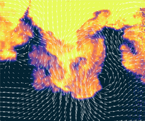
Figure 4 shows an example of the interface evolution captured in a HS experiment run, showing snapshots as a function of time every 5 frames.

Figure 4. Example evolution of the mixing layer after reshock. The light gas ( ${\rm He} + {\rm Acetone}$) mole fraction is shown overlaid with two-dimensional velocity vectors.
4.1. Power spectra
Following Schilling & Latini (Reference Schilling and Latini2010), the power spectra are integrated over the mixing layer such that  $\varLambda _{\xi }(k_x^{+}, h^{+}) = \int ^{\infty }_{-\infty } E_{\xi }\,\mathrm {d}z^{+}$ (here, the limits are $\pm \infty$ rather than the bubble and spike heights although, in practice, the limits are the bounds of the field of view of the experiment). The parameter $\varLambda _{\xi }$, shown in figure 5(a), is a measure of the magnitude of fluctuations at a given wavenumber with a smaller magnitude indicating weaker fluctuations from the mean and a more fully mixed state and $\varLambda _{w}$ is a measure of the kinetic energy at a given wavenumber, and is shown in figure 5(b).

Figure 5. Ensemble HS integrated power spectra. (a) Integrated scalar power spectrum. (b) Integrated kinetic power spectrum. Here,  $h^+$ plays the role of time for this mixing system. Integration is performed in the inhomogeneous direction.
For both  $\varLambda _{\xi }$ and $\varLambda _{w}$, energy is concentrated at smaller wavenumbers around the integral scale. A steady increase in energy over time is seen in $\varLambda _{\xi }$, showing a growth in bulk structures. For $\varLambda _{w}$ a deposition of kinetic energy is seen followed by a slow decay. A similar behaviour can be seen in figure 12 of Tritschler et al. (Reference Tritschler, Olson, Lele, Hickel, Hu and Adams2014) and figure 5(a) of Carter et al. (Reference Carter, Pathikonda, Jiang, Felver, Roy and Ranjan2019).
Figure 6 explores the coarse measures of the spectra introduced in § 3.2. Figures 6(a) and 6(c) show joint probability density functions ( j.p.d.f.s) and figures 6(b) and 6(d) show conditional probability density functions (c.p.d.f.s).

Figure 6. The HS results: (a) j.p.d.f. of spectral Schmidt number and scalar spectral slope; (b) conditional p.d.f. of scalar spectral slope given a spectral Schmidt number. (White line: Gibson Reference Gibson1968, (46).) (c) The j.p.d.f. of the spectral Reynolds number and the kinetic spectral slope. (d) Conditional p.d.f. of the spectral Reynolds number and the kinetic spectral slope.
In particular, figure 6(a) shows the j.p.d.f. of the turbulent Schmidt number and the scalar spectral slope. A peak in the j.p.d.f. can be seen where the scalar slope is approximately between  $-8/3$ and $-10/3$ and the turbulent Schmidt number is between $0.3$ and $0.4$, which aligns with the estimate of the material Schmidt number of 0.3. Figure 6(b) shows the c.p.d.f., which represents what the expected spectral slope is for a given turbulent Schmidt number. The result here is close to the interpolation formula by Gibson (Reference Gibson1968) ((46) in that paper), providing some encouragement to the proposition made in § 3.2 that, with the flow being far from HIT, the turbulent Schmidt number is appropriate to use in place of the material Schmidt number to determine expected behaviour.
Figure 6(c) shows the j.p.d.f. of turbulent Reynolds number and kinetic spectral slope. A peak can be seen at a slope between  $-5/3$ and $-2$ at an $Re_{\tau }$ between $20$ and $25$. The c.p.d.f. in figure 6(d) points to a weak dependence of the kinetic spectral slope on the turbulent Reynolds number, although it is difficult to draw conclusions at the lowest and highest $Re_{\tau }$ due to the lower number of observations available to generate the distribution there due to the turbulent Reynolds number over all measurements being close to the peak.
Figure 7 shows the same measurement as figure 6 but for the SS data set. Very similar structures and values and trends are visible in the Schmidt number-based plots, 7(a) and 7(b). The Reynolds number-based plots show a peak at a slightly lower value than the HS results in plot 6(c). Figure 7(d) shows a similar trend for the small  $Re_{\tau }$ range; however, a similar problem occurs with fewer instances to produce statistics for the higher $Re_{\tau }$ values.

Figure 7. The SS results: (a) j.p.d.f. of spectral Schmidt number and scalar spectral slope; (b) conditional p.d.f. of scalar spectral slope given a spectral Schmidt number. (White line: Gibson Reference Gibson1968, (46).) (c) The j.p.d.f. of the spectral Reynolds number and the kinetic spectral slope. (d) Conditional p.d.f. of the spectral Reynolds number and the kinetic spectral slope.
4.2. Partition of energy
Equation (3.7) describes the partition of the change in scalar energy over a given time interval. For this study, the dimensionless time interval is the regime of linear growth of the mixing width for all experiments from  $\ln h^+ = 0$ to $\ln h^{+} = 1.6$. The individual terms are plotted in figure 8 and defined in the Appendix. The time period represented here begins after the reflected shock has fully traversed the mixing layer; it includes the passage of an expansion wave and ends at the latest dimensionless time available before the arrival of a compression wave from above. This analysis is only possible with the time-resolved HS data set.

Figure 8. The terms of the transport of fluctuating scalar energy (3.7) over the linear growth regime from  ${h}/{h_0}=1$ to $5$ for the HS data set. Here, $\Delta E_{\xi }$ is the change in scalar energy over linear growth regime, $P_{\xi }$ is the production of scalar energy, $T_{x\xi }$ is the homogeneous convective transport, $\varPi _{z\xi }$ is the inhomogeneous convective flux, $D_{x\xi }$ is the homogeneous diffusion term, $D_{z\xi }$ is the inhomogeneous diffusion term and $X_{\xi }$ is the dissipation.
The total increase in energy, i.e. the increase in fluctuations away from the spanwise mean,  $\Delta E_{\xi }$, is concentrated at larger wavelengths, of the order of the shock tube width, which correspond to the growth and transport of bulk structures. This is evident in the plot of the production term $P_{\xi }$, which represents the transfer of energy from the mean gradient of the scalar field to the fluctuations via the correlation of streamwise velocity fluctuations and scalar fluctuations. The homogeneous transport term $T_{x\xi }$ describes how energy is transported in wavenumber space, where above and below the interface energy is being transported from larger wavelengths to smaller wavelengths ( $T_{x\xi }<0$) while in the centre of the mixing layer energy is being transported to larger wavelengths ( $T_{x\xi }>0$). The inhomogeneous transport flux $\varPi _{z\xi }$ shows how scalar energy is transported away from the centre of the mixing layer with a larger amount of energy transported in the negative z-direction than toward the positive z-direction above the interface. This asymmetry in energy transport is seen in Thornber & Zhou (Reference Thornber and Zhou2012) and is explained as an Atwood number effect. The homogeneous diffusion, $D_{x\xi }$ measures the rate of diffusing scalar energy from large to small wavelengths, while the inhomogeneous diffusion term $D_{z\xi }$ describes how energy is diffused in the vertical direction. The form makes sense as roughly the second derivative of a Gaussian such that energy is taken from the centre of the mixing layer and diffused to above and below the interface. Here, $X_{\xi }$ is the dissipation term and represents the removal of scalar energy which appears to occur at longer wavelengths where the gradients are largest.
4.3. Time evolution
To compare the HS and SS data sets further, here, the time evolution of the production and homogeneous transport terms are shown in figure 9.

Figure 9. Comparison of the production and transport flux between HS and SS experiments at comparable experiment times.
The same structures as discussed in § 4.2, referring to figure 8, appear here, where production occurs around the centroid of the mixing layer with asymmetry appearing. The flux term,  ${\rm \pi} _{\xi } = \int _{0}^{kW} T_{\xi x}\,\mathrm {d}k^+$, shows a positive flux above and below the interface with a negative flux along the centreline of the mixing layer. The structures seem to correlate, and the values are comparable; however, some of the details are different.
Cook & Zhou (Reference Cook and Zhou2002) calculate the time-varying dissipation, production and transport in non-scaling coordinates for an RTI problem. The production term of the system is very different between the RTI and RMI, so differences are expected in the temporal behaviour; however, transport and dissipation have the same mathematical structure. They do not separate terms by directionality, but comparison can be made with dominant terms. They find similar trends, with dissipation occurring at short wavelengths in the centre of the mixing layer and transport reaching peaks at long wavelengths, with positive values above and below the interface and negative values in the centre of the mixing layer.
Figure 10 shows the evolution of the terms of the spatially integrated total scalar energy transport equation (3.8) as a function of wavenumber and time. The peak of the integrated production, which is centred around the mean of the integral scales of the scalar and kinetic spectra, shows a steady growth after reshock before reaching a peak value and steadily decaying. The transport between scales is more complex. Initially, small amounts of transport occur after reshock. However, energy quickly begins being transported from large scales to small scales. Phase reversal allows a short duration of bulk transport of energy from small scales to large scales before the linear growth regime continues to drive the transport toward a profile that more closely matches an equilibrium turbulence profile such that, at the later times, energy is transporting from large scales toward the intermediate scales, and from small scales back toward intermediate scales. The LES results of Zeng et al. (Reference Zeng, Pan, Sun and Ren2018) show a very similar structure for the kinetic flux term as functions of wavenumber and time. The diffusion spectrum grows with the scalar power spectrum, but its amplitude shows it to be the subdominant method of energy transport compared with the convective transport term. In this far from equilibrium setting, the dissipation spectrum shows a steadily growing peak around the peak of the production spectrum; however, it is a strongly subdominant budget term. Production is the dominant term over the whole linear growth regime, while the convective transport term steadily begins to enable transport of energy to smaller wavelengths.

Figure 10. Time evolution of the terms in (3.8) as a function of wavenumber for the HS data set. The colour denotes the change in  $\ln (h^+)$, which is the dimensionless time. The evolution of the scalar and velocity power spectra are shown for reference. Here, $\hat {P}_{\xi }$ is the production of scalar energy, $\hat {T}_{xi}$ is the convective transport, $\hat {D}_{\xi }$ is the diffusion term and $\hat {X}_{\xi }$ is the dissipation.
5. Conclusions
The results of two sets of experiments were presented, both simultaneous PLIF and PIV, one set SS and one set time resolved. The terms in the evolution equations for the scalar and density-weighted kinetic energy spectra in a reshock RMI environment were presented. The scalar spectral index was shown, for both sets of experiments, to approximately follow the equation given by Gibson (Reference Gibson1968) as a function of effective Schmidt number, while the kinetic energy spectral index was shown to be approximately constant over the observed effective Reynolds number range and close to the Kolmogorov  $-5/3$ scaling. The partition of energy in the linear growth regime between the terms of the transport equation of the scalar power spectra was presented. A comparison of both HS and SS experiments shows a consistency of structures appearing, although IC structure dependence is suggested as a reason for the variation in the details of the evolution of the production and transport terms. This work suggests that the effective Schmidt number used here may be a useful parameter to work with to aid in the construction of spectral closure models, while the reported partitions of energy over the linear growth regime provide fields that will be useful for the comparison of RM and RT experiments at other conditions and simulations. Future work may want to expand the parameter space to see how the reported quantities behave as a function of shock strength and Atwood number.
Acknowledgements
The authors would like to thank Dr J. Herzog (now at the University of Michigan) for his invaluable assistance in the set-up of the HS laser system.
Funding
This work is supported by the US DOE/NNSA through grant number DE-NA0003932.
Declaration of interests
The authors report no conflict of interest.
Appendix. Partition of energy
The terms plotted in figure 8 are defined below. The integrals are taken from  $0$ to $5$ where ${h}/{h_0} = 5$ is the limit of the linear growth regime for all HS experiments
 \begin{gather} \left.\begin{gathered} P_{\xi}(z^{+},k_x^{+}) = \int_{0}^{\ln 5} \mathcal{P}\,\mathrm{d}\ln h^{+}\\ \hat{P}_{\xi}(k_x^{+}, h^{+}) = \int_{-\infty}^{\infty} \mathcal{P}\,\mathrm{d}z^{+}, \end{gathered}\right\} \end{gather}
 \begin{gather} \left.\begin{gathered} T_{x\xi}(z^{+},k_x^{+}) = \int_{0}^{\ln 5 } \mathcal{T}_{x\xi}\,\mathrm{d}\ln h^{+}\\ \hat{T}_{\xi}(k_x^{+}, h^{+}) = \int_{-\infty}^{\infty} \mathcal{T}_{x\xi}\,\mathrm{d}z^{+}, \end{gathered}\right\} \end{gather}
 \begin{gather} \varPi_{z\xi}(z^{+},k_x^{+}) = \int_{-\infty}^{z^+} \int_{0}^{\ln 5} \mathcal{T}_{z\xi}\, \mathrm{d}\ln h^{+}\,{\rm d}z^+, \end{gather}
 \begin{gather} \left.\begin{gathered} D_{x\xi}(z^{+},k_x^{+}) = \int_{0}^{\ln 5} \mathcal{D}_{x\xi}\,\mathrm{d}\ln h^{+}\\ \hat{D}_{\xi}(k_x^{+}, h^{+}) = \int_{-\infty}^{\infty} \mathcal{D}_{x\xi}\,\mathrm{d}z^{+}, \end{gathered}\right\} \end{gather}
 \begin{gather} D_{z\xi}(z^{+},k_x^{+}) = \int_{0}^{\ln 5} \mathcal{D}_{z\xi}\,\mathrm{d}\ln h^{+}, \end{gather}
 \begin{gather} \left.\begin{gathered} X_{\xi}(z^{+},k_x^{+}) = \int_{0}^{\ln 5} \chi_{\xi}\,\mathrm{d}\ln h^{+} \\ \hat{X}_{\xi}(k_x^{+}, h^{+}) = \int_{-\infty}^{\infty} \chi_{\xi}\,\mathrm{d}z^{+}. \end{gathered}\right\} \end{gather}


 Open access