


1 Introduction
Air entrainment occurs and plays important roles in both natural processes and engineering applications. Quantifying the total volume, size distribution and scale dependence of entrained air in free-surface turbulence is key to modelling the natural air entrainment and gas transfer across the air–sea interface in ocean breaking waves (Deane & Stokes Reference Deane and Stokes2002) and the design of aeration cascades to increase oxygen concentration in water treatment plants (Chanson Reference Chanson1996).
To date, much of the understanding of air entrainment is in the context of breaking waves. Deane & Stokes (Reference Deane and Stokes2002) measured the bulk bubble-size spectra (per unit volume)  $N(r)$ inside breaking waves in the laboratory. In the initial acoustic phase, when entrainment primarily occurs, they identified two distinct power-law regimes of $N(r)$, depending on the bubble size $r$. For $r\gtrsim 1~\text{mm}$, $N(r)\propto r^{-10/3}$, while for $r\lesssim 1~\text{mm}$, $N(r)\propto r^{-3/2}$. They calculated the Hinze scale $r_{H}$ (Hinze Reference Hinze1955) using
 $$\begin{eqnarray}r_{H}=2^{-8/5}(We_{c}\,\unicode[STIX]{x1D70E}/\unicode[STIX]{x1D70C})^{3/5}\unicode[STIX]{x1D716}^{-2/5},\end{eqnarray}$$
 where  $We_{c}\approx 4.7$ is the critical Weber number for bubble breakup by turbulence predicted from experiments (Lewis Reference Lewis1982; Martínez-Bazán, Montanes & Lasheras Reference Martínez-Bazán, Montanes and Lasheras1999). Using the fact that $r_{H}$ in the experiments was close to the separation scale $r_{0}\sim 1~\text{mm}$, they argued that $r_{0}$ is $r_{H}$. In the quiescent phase ( ${\sim}1.5~\text{s}$ after the acoustic phase) the bubble plume evolved rapidly under the influence of advection, turbulent diffusion and buoyant degassing, with an accompanying (more complex) evolution of $N(r)$. For the air entrainment phase, other researchers (Loewen, O’Dor & Skafel Reference Loewen, O’Dor and Skafel1996; Rojas & Loewen Reference Rojas and Loewen2007; Blenkinsopp & Chaplin Reference Blenkinsopp and Chaplin2010; Deike, Melville & Popinet Reference Deike, Melville and Popinet2016; Wang, Yang & Stern Reference Wang, Yang and Stern2016) confirm the power-law dependence $N(r)\propto r^{-10/3}$ for larger bubbles in breaking waves experiments and simulations. For the regime $r\lesssim r_{0}$, Rojas & Loewen (Reference Rojas and Loewen2007) and Wang et al. (Reference Wang, Yang and Stern2016) obtained similar results to those of Deane & Stokes (Reference Deane and Stokes2002).
Several parameterizations have been proposed for the air entrainment phase  $N(r)$. Garrett, Li & Farmer (Reference Garrett, Li and Farmer2000) performed a dimensional analysis in which $N(r)$ (dimension $L^{-4}$) is assumed to depend on the turbulence dissipation rate $\unicode[STIX]{x1D716}$, the average rate of supply of air $Q$ and the bubble radius $r$, and obtained a parameterization of the form
 $$\begin{eqnarray}N(r)\propto Q\unicode[STIX]{x1D716}^{-1/3}r^{-10/3}.\end{eqnarray}$$
 Deane & Stokes (Reference Deane and Stokes2002) pointed out that (1.2) is valid only for  $r\gtrsim r_{H}$. For $r\lesssim r_{H}$, surface tension becomes important, requiring a different scale dependence. Performing a similar dimensional analysis for $r<r_{H}$, and assuming $N(r)$ is a multiplicative function of surface tension $\unicode[STIX]{x1D70E}$, liquid density $\unicode[STIX]{x1D70C}$, jet velocity $v$ and bubble radius $r$, they obtain a $N(r)$ scaling for these smaller bubbles:
 $$\begin{eqnarray}N(r)\propto Q(\unicode[STIX]{x1D70E}/\unicode[STIX]{x1D70C})^{-3/2}v^{2}r^{-3/2}.\end{eqnarray}$$
 The models (1.2) and (1.3) originate from dimensional analysis and it is not clear if they reflect all of the underlying physical mechanism(s) of air entrainment. In particular, the inverse dependence on  $\unicode[STIX]{x1D716}$ in (1.2) and the non-dependence on $\unicode[STIX]{x1D716}$ in (1.3) of $N(r)$ seem non-physical. Since turbulence provides energy for bubble entrainment (Brocchini & Peregrine Reference Brocchini and Peregrine2001), a greater $\unicode[STIX]{x1D716}$ should increase the magnitude of $N(r)$. Deike et al. (Reference Deike, Melville and Popinet2016) argued that $Q$ should itself be a function of $\unicode[STIX]{x1D716}$, and the combination of $Q$ and $\unicode[STIX]{x1D716}^{-1/3}$ in (1.2) could lead to a positive exponent for $\unicode[STIX]{x1D716}$. Similarly for (1.3), we can obtain a scaling of $\unicode[STIX]{x1D716}^{2/3}$ instead of $\unicode[STIX]{x1D716}^{0}$ if $\unicode[STIX]{x1D716}\propto v^{3}/D_{j}$, with $D_{j}$ the jet diameter. Finally, the identification of the regime separation scale $r_{0}$ with the Hinze scale $r_{H}$, while physically plausible, is not definitive. The possibility that $r_{0}$ derives from other relevant physical scales of the problem cannot be ruled out.
In this paper, we investigate the air entrainment across a free surface induced by underlying strong free-surface turbulence (SFST), specifically its bubble-size distribution and scale dependence. We define  ${\mathcal{N}}_{a}^{E}(r)$ (dimension $L^{-3}$) as the bubble-size spectrum per unit mean interface area (over a unit time in the quasi-steady air entrainment process). Through energy arguments, we show (in § 2) that ${\mathcal{N}}_{a}^{E}(r)$ follows two power-law regimes, depending on bubble size $r$, separated by a bubble-size length scale $r_{0}$. For $r>r_{0}$, ${\mathcal{N}}_{a}^{E}(r)$ scales as $g^{-1}\unicode[STIX]{x1D716}^{2/3}r^{-10/3}$, describing a gravity-dominated entrainment regime. For $r<r_{0}$, ${\mathcal{N}}_{a}^{E}(r)$ scales as $(\unicode[STIX]{x1D70E}/\unicode[STIX]{x1D70C})^{-1}\unicode[STIX]{x1D716}^{2/3}r^{-4/3}$, describing a surface-tension-dominated entrainment regime. We show that $r_{0}$ is in fact the capillary scale $r_{c}=1/2\sqrt{\unicode[STIX]{x1D70E}/\unicode[STIX]{x1D70C}g}$, independent of flow parameters such as $\unicode[STIX]{x1D716}$; and hence not related to the Hinze scale $r_{H}$ as is often assumed (Deane & Stokes Reference Deane and Stokes2002; Wang et al. Reference Wang, Yang and Stern2016). Inspired by the diagram of the ( $L$,
$L$,  $q$)-plane in Brocchini & Peregrine (Reference Brocchini and Peregrine2001), we derive a ( $r$,
$r$,  $\unicode[STIX]{x1D716}$)-plane prediction of when air entrainment occurs in free-surface turbulence (FST). The resulting regime map predicts a critical dissipation value $\unicode[STIX]{x1D716}_{cr}$ below which air entrainment is suppressed, thus demarcating weak FST (WFST) from SFST in terms of air entrainment. Like $r_{0}$, $\unicode[STIX]{x1D716}_{cr}$ depends only on the physical constants $g$ and $\unicode[STIX]{x1D70E}/\unicode[STIX]{x1D70C}$.
In § 3, we confirm our theoretical predictions using high-resolution direct numerical simulations (DNS) of canonical FST flows, solving three-dimensional two-phase incompressible Navier–Stokes equations with a fully nonlinear interface resolved by the conservative volume-of-fluid method (cVOF) (Weymouth & Yue Reference Weymouth and Yue2010). We note that the surface entrainment size spectrum  ${\mathcal{N}}_{a}^{E}(r)$ has a direct relationship to the (bulk) volume size spectrum $N_{a}(r)$ generally measured in experiments and simulations by labelling and sizing bubbles in the bulk. For a relatively short time after the onset of entrainment, before subsurface mechanisms come into play, $N_{a}(r)$ closely resembles ${\mathcal{N}}_{a}^{E}(r)$ in terms of the power-law regimes and slopes. With increasing time, $N_{a}(r)$ evolves (primarily) as a result of turbulent bubble fragmentation and degassing, and can become qualitatively different from ${\mathcal{N}}_{a}^{E}(r)$ (Yu et al. Reference Yu, Hendrickson, Campbell and Yue2019). We perform DNS over a range of Froude ( $Fr$) and Weber ( $We$) numbers for the FST and obtain $N_{a}(r)$ at a relatively early time. The DNS confirms the key predictions of the scaling model: the gravity- and surface-tension-dominated power-law regimes and slopes; the separation scale $r_{0}=r_{c}$ ( ${\approx}1.5~\text{mm}$ for an air–water interface in Earth gravity); and the scaling with $\unicode[STIX]{x1D716}^{2/3}$ (over the range we considered). Plotting the DNS data on the $\unicode[STIX]{x1D716}$– $r$ regime map also confirms the critical dissipation for air entrainment, $\unicode[STIX]{x1D716}_{cr}\sim O(10^{-2}~\text{m}^{2}~\text{s}^{-3})$, for an air–water interface and Earth gravity.
2 Scaling for bubble-size distribution of air entrainment in SFST
To model the size spectrum of entrainment across a given free-surface area, we consider the entrainment size spectrum  ${\mathcal{N}}_{a}^{E}(r)$, of dimension $L^{-3}$, where ${\mathcal{N}}_{a}^{E}(r^{\prime })\unicode[STIX]{x1D6FF}r$ is the number of bubbles of (equivalent) radius $r^{\prime }<r<r^{\prime }+\unicode[STIX]{x1D6FF}r$ entrained per unit (mean) free-surface area. For simplicity, we assume quasi-steady air entrainment over unit time. A physical/mechanistic derivation for the scaling of ${\mathcal{N}}_{a}^{E}(r)$ through an energy argument requires two assumptions. First, we assume that the only source of bubble generation is the surrounding turbulence (Brocchini & Peregrine Reference Brocchini and Peregrine2001). Second, we assume that the void fraction of bubbles is small and does not affect the dynamics of the bulk water turbulence (Garrett et al. Reference Garrett, Li and Farmer2000).

Figure 1. (a) Scenarios considered in the energy argument for bubble entrainment. (b) Sheared free-surface turbulent flow for DNS. Yu et al. (Reference Yu, Hendrickson, Campbell and Yue2019) contains full simulation details.
Consider a simplified entrainment scenario of a static spherical air bubble of radius  $r$ formed at a depth $2r\unicode[STIX]{x1D6FC}$ under the free surface (a change in energy between Scenario 1 and 2 sketched in figure 1a). We assume the constant $\unicode[STIX]{x1D6FC}$ is of order 1 to account for this simplification. The minimum energy required to entrain such a bubble, $E_{b}(r)$, is the sum of the potential energy and the surface energy:
 $$\begin{eqnarray}E_{b}(r)=g\frac{4}{3}\unicode[STIX]{x03C0}r^{3}2r\unicode[STIX]{x1D6FC}+\frac{\unicode[STIX]{x1D70E}}{\unicode[STIX]{x1D70C}}4\unicode[STIX]{x03C0}r^{2}.\end{eqnarray}$$
 The total number of bubbles of radius  $r$ entrained across a (initial) surface area $A_{h}$ is ${\mathcal{N}}_{a}^{E}(r)A_{h}\,\text{d}r$ and the total energy required for entrainment of these bubbles is
 $$\begin{eqnarray}{\mathcal{N}}_{a}^{E}(r)A_{h}\,\text{d}rE_{b}(r)={\mathcal{N}}_{a}^{E}(r)A_{h}\,\text{d}r\left(g\frac{4}{3}\unicode[STIX]{x03C0}r^{3}2r\unicode[STIX]{x1D6FC}+\frac{\unicode[STIX]{x1D70E}}{\unicode[STIX]{x1D70C}}4\unicode[STIX]{x03C0}r^{2}\right).\end{eqnarray}$$
 Using our first assumption, this amount of energy is supplied by turbulence over a near-surface region of depth  $r$ (around the entrained bubbles). Defining $E(k)$ as the turbulence energy spectrum, the turbulence energy per unit volume at length scale $1/k$ is given by $|E(k)\,\text{d}k|$. We argue that the turbulence of length scale $1/k$ is primarily responsible for the entrainment of bubbles of radius $r\sim 1/k$. The available energy supplied by near-surface turbulence for entrainment within a volume $A_{h}r$ is proportional to
 $$\begin{eqnarray}|E(k)\,\text{d}k|A_{h}r\propto |E(r^{-1})\,\text{d}r^{-1}|A_{h}r=E(r^{-1})r^{-2}\,\text{d}rA_{h}r.\end{eqnarray}$$
From an energy argument, (2.2) is proportional to (2.3) which yields
 $$\begin{eqnarray}{\mathcal{N}}_{a}^{E}(r)A_{h}\,\text{d}r\left(g\frac{4}{3}\unicode[STIX]{x03C0}r^{3}2r\unicode[STIX]{x1D6FC}+\frac{\unicode[STIX]{x1D70E}}{\unicode[STIX]{x1D70C}}4\unicode[STIX]{x03C0}r^{2}\right)\propto E(r^{-1})r^{-2}\,\text{d}rA_{h}r.\end{eqnarray}$$
 For SFST, the characteristic large surface deformations (and large  $Fr$ and $We$) weaken the free-surface boundary conditions, resulting in essentially isotropic near-surface turbulence (Yu et al. Reference Yu, Hendrickson, Campbell and Yue2019). Thus, the Kolmogorov spectrum $E(r^{-1})\propto \unicode[STIX]{x1D716}^{2/3}r^{5/3}$ provides the near-surface turbulence energy spectrum (this is also confirmed in the DNS, see figure 4). Using the Kolmogorov spectrum, (2.4) becomes
 $$\begin{eqnarray}{\mathcal{N}}_{a}^{E}(r)\propto \left(\frac{2}{3}gr\unicode[STIX]{x1D6FC}+\frac{\unicode[STIX]{x1D70E}}{\unicode[STIX]{x1D70C}}\frac{1}{r}\right)^{-1}\unicode[STIX]{x1D716}^{2/3}r^{-7/3}.\end{eqnarray}$$
For flows with different underlying turbulence spectra (for example, due to large bubble density, Alméras et al. Reference Alméras, Mathai, Lohse and Sun2017), the predicted bubble-size spectra will be modified accordingly.
From (2.5), we observe two regimes of entrainment by considering  $f(r)=(2/3)gr\unicode[STIX]{x1D6FC}+(\unicode[STIX]{x1D70E}/\unicode[STIX]{x1D70C})(1/r)$. For large $r$, gravity dominates $f(r)$ as $(2/3)gr\unicode[STIX]{x1D6FC}$ is large, and (2.5) becomes
 $$\begin{eqnarray}{\mathcal{N}}_{a}^{E}(r)\propto g^{-1}\unicode[STIX]{x1D716}^{2/3}r^{-10/3}.\end{eqnarray}$$
 For small  $r$, surface tension dominates $f(r)$ as $(\unicode[STIX]{x1D70E}/\unicode[STIX]{x1D70C})(1/r)$ is large, and (2.5) becomes
 $$\begin{eqnarray}{\mathcal{N}}_{a}^{E}(r)\propto (\unicode[STIX]{x1D70E}/\unicode[STIX]{x1D70C})^{-1}\unicode[STIX]{x1D716}^{2/3}r^{-4/3}.\end{eqnarray}$$
 The scale separating the two regimes  $r_{0}$ occurs when the two terms in $f(r)$ are comparable at $r_{0}=\sqrt{1.5\unicode[STIX]{x1D70E}/\unicode[STIX]{x1D6FC}\unicode[STIX]{x1D70C}g}$. This capillary scale $r_{0}\approx r_{c}=0.5\sqrt{\unicode[STIX]{x1D70E}/\unicode[STIX]{x1D70C}g}$ corresponds to a balance between gravity and surface tension forces, or Bond number $Bo\equiv \unicode[STIX]{x1D70C}g(2r_{c})^{2}/\unicode[STIX]{x1D70E}=1$.
We note that (2.6) and (2.7) are also obtained directly from dimensional analysis using the relevant set of physical parameters. In contrast to Garrett et al. (Reference Garrett, Li and Farmer2000) and Deane & Stokes (Reference Deane and Stokes2002), for free-surface air entrainment, the size spectrum per unit surface area,  ${\mathcal{N}}_{a}^{E}(r)$ (dimension $L^{-3}$), is powered by the FST kinetic energy measured by $\unicode[STIX]{x1D716}$ ( $L^{2}T^{-3}$). This is balanced by gravity $g$ (
$g$ ( $LT^{-2}$) and surface tension $\unicode[STIX]{x1D70E}/\unicode[STIX]{x1D70C}$ ( $L^{3}T^{-2}$). Matching dimensions, we immediately obtain the scaling results for the respective size regimes.
Several remarks are in order. First, for the  $r>r_{0}$ regime, the power-law slope $r^{-10/3}$ happens to coincide with that of Garrett et al. (Reference Garrett, Li and Farmer2000) – for example, (1.2). However, the underlying physical processes in these two models are different in that Garrett et al. (Reference Garrett, Li and Farmer2000) considered a cascade scenario of bubble fragmentation rather than air entrainment driven by surface turbulence as in our model. In fact, the slopes of the two power-law regimes in (2.6) and (2.7) result directly from the power-law slope of the near-surface isotropic SFST energy spectrum. One physical explanation for the coincidental similarity of the power-law slope of our model and Garrett et al. (Reference Garrett, Li and Farmer2000) is to frame the air–water boundary of an initially large cavity immersed in an isotropic turbulent field as a free surface with underlying isotropic near-surface turbulence. In this context, the bubble generation process through fragmentation is similar to turbulence air entrainment (Hendrickson et al. Reference Hendrickson, Weymouth, Yu and Yue2019). Second, for $r<r_{0}$ in the surface-tension-dominated regime, the power-law slope in (2.7) differs (slightly) from the model of Deane & Stokes (Reference Deane and Stokes2002) in (1.3). Third, the (positive exponent) dependence on turbulence dissipation rate ${\sim}\unicode[STIX]{x1D716}^{2/3}$ in the current models (2.6) and (2.7) is physically reasonable compared to that of (1.2) ( ${\sim}\unicode[STIX]{x1D716}^{-1/3}$) and (1.3) ( ${\sim}\unicode[STIX]{x1D716}^{0}$). In the current model, stronger surface turbulence leads to more entrainment. Finally, the separation scale $r_{0}$ is independent of flow parameters and not strictly related to the Hinze scale $r_{H}$ as generally assumed (without strict theoretical consideration). The present theory provides a direct argument that $r_{0}$ is the physical capillary scale $r_{0}\approx r_{c}$, which, for an air–water interface under the influence of Earth gravity, is $r_{c}\approx 1.5~\text{mm}$.
As discussed in § 1, the scale dependence of the surface entrainment size spectrum  ${\mathcal{N}}_{a}^{E}(r)$ should be reflected in the underlying volume size spectrum $N_{a}(r)$ providing it is early enough in time, when fragmentation and degassing are not a factor. Figure 2 shows the theoretical prediction for
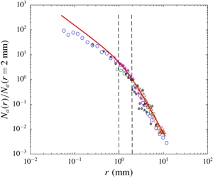
  ${\mathcal{N}}_{a}^{E}(r)$ in (2.5) superposed on available experimental and DNS data for $N_{a}(r)$ obtained for both breaking waves and SFST flows. For comparison of the spectral shape/slope, we normalize the magnitude of each dataset by its values at some (arbitrary) radius $r=2~\text{mm}$. Despite the fact that most of the datasets in figure 2 are from breaking waves, the scale dependence of the data appears to be well described by (2.5) for the entire range of $r$. We point out that in figure 2 the transition between the two regimes for most of the data occurs near $r_{0}=1$–2 mm, despite presumably different values of turbulent dissipation rates for the different datasets.

Figure 2. Comparison of  ${\mathcal{N}}_{a}^{E}(r)$ in (2.5) (with $\unicode[STIX]{x1D6FC}=6$) and the measured bubble-size spectrum $N_{a}(r)$ inside breaking waves from the literature. All the data and (2.5) are normalized by their own values at $r=2~\text{mm}$: ——, equation (2.5); ○, Deane & Stokes (Reference Deane and Stokes2002); ▫, Rojas & Loewen (Reference Rojas and Loewen2007); $Fr^{2}=21$, $We=2100$ and $Re=1200$ in § 3; ▵, Yu et al. (Reference Yu, Hendrickson, Campbell and Yue2019).
 Air entrainment in SFST is a result of two competing effects on the free surface: the disrupting effect of near-surface turbulence and the stabilizing effect from gravity and surface tension. Comparing the two effects provides criteria for the lower and upper bounds  $r_{l}$ and $r_{u}$ of bubble size that can be entrained. We argue that the lower bound $r_{l}$ corresponds to a scale where turbulence disturbance is much smaller than surface tension forces – that is, $We_{t}=\unicode[STIX]{x1D70C}\overline{v^{2}}(2r_{l})/\unicode[STIX]{x1D70E}=We_{l}$ ( $\ll 1$), where $\overline{v^{2}}\approx 2.0(\unicode[STIX]{x1D716}d)^{2/3}$ is the turbulence fluctuation over a distance $d=2r_{l}$; $r_{l}$ can be further written as
 $$\begin{eqnarray}r_{l}=2^{-8/5}(\unicode[STIX]{x1D70E}/\unicode[STIX]{x1D70C}\,We_{l})^{3/5}\unicode[STIX]{x1D716}^{-2/5}.\end{eqnarray}$$
 Equation (2.8) is the same form as the Hinze scale (1.1), with  $We_{l}$ replacing $We_{c}$. Both $r_{l}$ and $r_{H}$ correspond to the critical length scales resulting from the competition between near-surface turbulence and surface tension forces. While the length scale $r_{H}$ is for bubbles with a stable spherical interface, $r_{l}$ is the length scale associated with the breakup of a free surface with a relatively unstable flat interface. As such, we expect $We_{l}\ll We_{c}$ (and consequently $r_{l}\ll r_{H}$).
We define the upper bound bubble length scale  $r_{u}$ similarly from the (turbulence) Froude number $Fr_{t}^{2}=\overline{v^{2}}/g(2r_{u})=Fr_{u}^{2}$ ( $\ll 1$), which yields
 $$\begin{eqnarray}r_{u}=4(Fr_{u}^{2}g)^{-3}\unicode[STIX]{x1D716}^{2}.\end{eqnarray}$$
 With the expressions (2.8) and (2.9) in terms of  $\unicode[STIX]{x1D716}$, we obtain a critical turbulent dissipation $\unicode[STIX]{x1D716}_{cr}$ when $r_{u}(\unicode[STIX]{x1D716}_{cr})=r_{l}(\unicode[STIX]{x1D716}_{cr})$, below which no entrainment would occur:
 $$\begin{eqnarray}\unicode[STIX]{x1D716}_{cr}=C_{\unicode[STIX]{x1D716}}g^{5/4}(\unicode[STIX]{x1D70E}/\unicode[STIX]{x1D70C})^{1/4}.\end{eqnarray}$$
 As with the separation scale  $r_{0}$ for ${\mathcal{N}}_{a}^{E}(r)$, $\unicode[STIX]{x1D716}_{cr}$ is a constant that depends only on the interface media and value of gravity. The upper and lower bounds (2.8) and (2.9) enable us to predict an $\unicode[STIX]{x1D716}$– $r$ regime map for bubble entrainment in FST (see figure 3, also see Brocchini & Peregrine (Reference Brocchini and Peregrine2001)). The dependencies of $r_{l}$ and $r_{u}$ on $\unicode[STIX]{x1D716}$ demarcate four regions in the ( $\unicode[STIX]{x1D716}$– $r$)-plane. The strong free-surface turbulence regime $(\unicode[STIX]{x1D716}>\unicode[STIX]{x1D716}_{cr})$ is where entrainment occurs within the size range $r_{l}<r<r_{u}$, which we denote Region 2 in figure 3. The bubble-size range increases with $\unicode[STIX]{x1D716}$. Turbulence will not entrain bubbles outside of this size range due to dominant gravity or surface tension forces. The weak free-surface turbulence regime $(\unicode[STIX]{x1D716}<\unicode[STIX]{x1D716}_{cr})$ is where no entrainment occurs for three different physical reasons. In Region 1, $r<r_{l}$ and surface tension forces stabilize the free surface. In Region 3, $r>r_{u}$ and strong gravity forces suppress air entrainment. In Region 0, both gravity and surface tension forces suppress entrainment.

Figure 3. Conceptual  $\unicode[STIX]{x1D716}$– $r$ regime map to predict FST-driven entrainment for an air–water interface under Earth gravity: $r_{l}$ of (2.8); $r_{u}$ of (2.9); with $\unicode[STIX]{x1D716}_{c}\approx 0.02~\text{m}^{2}~\text{s}^{-3}$ and $r_{c}\approx 1.5~\text{mm}$. For DNS data: $We_{l}\equiv 0.1$ and $Fr_{u}^{2}\equiv 0.1$ (consistent with physical arguments).
3 Direct numerical simulations of FST
We perform DNS of a canonical problem of three-dimensional incompressible two-phase (air and water) viscous turbulent flow with turbulent kinetic energy supplied by a sheared underlying bulk water flow (see figure 1b). Extensive documentation of the turbulence characteristics of this flow exists for non-entraining WFST at low  $Fr$ (Shen et al. Reference Shen, Zhang, Yue and Triantafyllou1999; Shen, Triantafyllou & Yue Reference Shen, Triantafyllou and Yue2000, Reference Shen, Triantafyllou and Yue2001; Shen & Yue Reference Shen and Yue2001) and air-entraining SFST at high $Fr$ (Yu et al. Reference Yu, Hendrickson, Campbell and Yue2019). We solve the three-dimensional two-phase incompressible Navier–Stokes equations with a fully nonlinear interface resolved by the cVOF method (Weymouth & Yue Reference Weymouth and Yue2010), which conserves volume to machine accuracy. Yu et al. (Reference Yu, Hendrickson, Campbell and Yue2019) provides the details of numerical implementations and verifications. For the data presented here, the mean shear-flow depth $L$ and velocity deficit $U$ are the characteristic length and velocity scales and normalize all the variables unless otherwise stated, with $Fr^{2}=U^{2}/gL$, $We=\unicode[STIX]{x1D70C}U^{2}L/\unicode[STIX]{x1D70E}$ and $Re=UL/\unicode[STIX]{x1D708}$. The domain size is $6^{3}$ and the grid size $\unicode[STIX]{x1D6E5}\approx 0.01$. In the analyses below, we report (only) bubbles that are considered resolved in the presence of surface tension in the DNS corresponding to equivalent diameter $2r\gtrsim 7\unicode[STIX]{x1D6E5}$. The unreported entrained volume is ${\lesssim}1\,\%$ for all cases. For SFST, we present results for two high-resolution DNS, both with $Bo=\unicode[STIX]{x1D70C}gL^{2}/\unicode[STIX]{x1D70E}=100$. DNS-1 has parameters $Fr^{2}=21$, $We=2100$ and $Re=1200$ and DNS-2 has $Fr^{2}=24.64$, $We=2464$ and $Re=1300$. We note that for constant $g$,
$g$,  $\unicode[STIX]{x1D70E}/\unicode[STIX]{x1D70C}$ and $\unicode[STIX]{x1D708}$, DNS-2 has a larger $U$ and the same $L$ as DNS-1.
The DNS results capture the evolution of air-entraining SFST corresponding to large  $Fr$ and $We$ (Yu et al. Reference Yu, Hendrickson, Campbell and Yue2019). Briefly, starting from a quiescent free surface, the FST grows rapidly due to production by the bulk flow mean shear, followed by a quasi-steady active entrainment SFST period, after which the FST eventually decays (and entrainment ceases) due to turbulence diffusion and dissipation. We report results within the quasi-steady active entrainment SFST period. In this period, turbulence forms vortical structures of different length scales near the free surface and entrains bubbles of different sizes (Yu et al. Reference Yu, Hendrickson, Campbell and Yue2019). Figure 4 shows the one-dimensional energy spectra of near-surface turbulence during the SFST period for DNS-1 (DNS-2 is similar). Consistent with the assumption in § 2, the turbulence shows isotropy, with the three components having comparable magnitudes and following the Kolmogorov $k^{-5/3}$ spectral slope.

Figure 4. One-dimensional near-surface energy spectrum  $E_{11}(k_{1})$ (——), $E_{22}(k_{1})$ (– – –), $E_{33}(k_{1})$ (— ⋅ —) at $t=56$ for DNS-1.
Figure 5 shows the volume bubble-size spectra  $N_{a}(r)$ for DNS-1 during the active entrainment period ( $r$ is normalized by the capillary scale $r_{c}$ for clarity). The measured bulk spectrum provides direct support of the scale dependencies of (2.6) and (2.7), respectively, for $r>r_{0}$ and $r<r_{0}$ with the separation scale $r_{0}\approx r_{c}$. We estimate $r_{H}$ (shown in figure 5) using the dimensionless form of (1.1), $r_{H}=2^{-8/5}(We_{c}/We)^{3/5}\unicode[STIX]{x1D716}^{-2/5}$, using the DNS-1 near-surface turbulence dissipation rate $\unicode[STIX]{x1D716}\sim O(10^{-3})$ and $We_{c}=4.7$. For DNS-1, $r_{H}$ is approximately three times greater than $r_{c}$, and this scale separation allows us to confirm that the separation scale between the two regimes is indeed $r_{0}\approx r_{c}$ and not $r_{H}$. For this particular DNS case, turbulence fragmentation of entrained bubbles should not have significant effects on $N_{a}(r)$ within the entrainment period, because $r_{H}$ is at the upper bound of the measured entrainment. We confirm this by comparing the three spectra at different times for $r<r_{H}$ in figure 5. This enables us to estimate ${\mathcal{N}}_{a}^{E}(r)$ using $N_{a}(r)$ with confidence. The inset of figure 5 shows $N_{a}(r)$ for both DNS-1 and DNS-2 averaged over the entrainment period. For DNS-2, $\unicode[STIX]{x1D716}$ is increased by a factor of 1.5. However, $r_{0}$ is the same for both DNS datasets and occurs at $r_{c}$ (which is the same for both DNS). This further confirms that $r_{0}$ between the two power-law entrainment regimes is in fact the capillary scale $r_{c}$ and not the Hinze scale $r_{H}$, which changes with $\unicode[STIX]{x1D716}$.

Figure 5. Volume bubble-size spectrum  $N_{a}(r)$ during the active entrainment period of DNS-1: ○, at a time sampled within the entrainment period; ▫, at a time sampled close to the end of entrainment period; *, average of $N_{a}(r)$ at every $tL/U=0.5$ within the entrainment period. Here $r_{c}=0.5\sqrt{\unicode[STIX]{x1D70E}/\unicode[STIX]{x1D70C}g}$ is the capillary length scale and $r_{H}$ is the Hinze scale in (1.1). The two theoretical power laws of $r^{-4/3}$ and $r^{-10/3}$ are represented by ——. The inset shows the average volume bubble-size spectrum $N_{a}(r)$ (within the entrainment period) for: *, DNS-1; $+$, DNS-2.
To confirm the scaling of the entrainment model with turbulent dissipation, we perform a series of lower-resolution DNS with  $\unicode[STIX]{x1D6E5}=0.027$ for FST with $Fr^{2}=10$, $We=50\,000$ and $Re=1000$, varying the slope of the initial mean shear profile to achieve different values for $\unicode[STIX]{x1D716}$. Figure 6 shows the linear dependence of the integral of averaged $N_{a}(r)$ (or entrained volume) plotted against $\overline{\unicode[STIX]{x1D716}^{2/3}}$ (averaged during the entrainment period), which confirms the positive exponent scaling of ${\mathcal{N}}_{a}^{E}(r)\propto \unicode[STIX]{x1D716}^{2/3}$ in (2.5). Linear regression obtains a horizontal intercept corresponding to $\overline{\unicode[STIX]{x1D716}^{2/3}}\approx 0.002$. When scaled by an air–water interface under Earth gravity, it provides an independent estimate of $\unicode[STIX]{x1D716}_{cr}\approx 0.03~\text{m}^{2}~\text{s}^{-3}$ that compares well to the $0.02~\text{m}^{2}~\text{s}^{-3}$ value obtained from figure 3.

Figure 6. Integral of  $N_{a}(r)$ over the resolved range of $r$ plotted against $\overline{\unicode[STIX]{x1D716}^{2/3}}$, normalized by $L$ and $U$ (♦). The average is during the entrainment period for DNS with $Fr^{2}=10$ and $We=50\,000$ and four variable shear profiles. ——: linear regression model $y=2.01x-0.00422$ with R-square 0.996.
Finally, we confirm the prediction of the  $\unicode[STIX]{x1D716}$– $r$ entrainment regime map, figure 3, using FST DNS over a broad range of $Fr^{2}$, $We$ and $\unicode[STIX]{x1D716}$ (by varying the initial mean shear profiles). We estimate the physical units of the characteristic length scale $L$ and near-surface turbulence dissipation rate $\unicode[STIX]{x1D716}$ using the defined values of $Fr^{2}$, $We$ and $Re$ (and assume Earth gravity and an air–water interface). The measured size range of entrainment as functions of $\unicode[STIX]{x1D716}$ for the different cases are superimposed onto the map in figure 3 (heavy lines). Notice that $r_{l}$ and $r_{u}$ in (2.8) and (2.9) assume an unbounded turbulence inertial range. For each DNS case, the range of the entrainment bubble size has a lower bound of $\unicode[STIX]{x1D6E5}$ and an upper bound of $L$ as well. This range of $(\unicode[STIX]{x1D6E5},L)$ is represented by dashed lines. The selected DNS cases with/without air entrainment correctly fall into the predicted regions of strong/weak FST, substantially confirming the predictions of § 2.
4 Conclusion
We perform theoretical and numerical investigations of air entrainment, and specifically the entrainment bubble-size distribution under SFST. Using arguments relating the energy required for bubble entrainment/formation and available turbulent kinetic energy in the SFST, we obtain a theoretical model for the surface entrainment bubble-size spectrum  ${\mathcal{N}}_{a}^{E}(r)$. The model describes two size regimes separated by a scale $r_{0}$, with ${\mathcal{N}}_{a}^{E}(r)\propto g^{-1}\unicode[STIX]{x1D716}^{2/3}r^{-10/3}$ for $r>r_{0}$, and ${\mathcal{N}}_{a}^{E}(r)\propto (\unicode[STIX]{x1D70E}/\unicode[STIX]{x1D70C})^{-1}\unicode[STIX]{x1D716}^{2/3}r^{-4/3}$ for $r<r_{0}$, where $r$ is the (equivalent) bubble radius, $g$ is gravity, $\unicode[STIX]{x1D70E}$ is the surface tension, $\unicode[STIX]{x1D70C}$ is the water density and $\unicode[STIX]{x1D716}$ is the turbulent dissipation rate of the SFST. From the model, we obtain that $r_{0}$ is the capillary scale $r_{c}$ ( ${\approx}1.5~\text{mm}$ for an air–water interface under Earth gravity), distinct from the Hinze scale $r_{H}$. We also propose an $\unicode[STIX]{x1D716}$– $r$ regime map to describe air entrainment in free-surface turbulent flows. The map predicts a critical value of the dissipation rate $\unicode[STIX]{x1D716}_{cr}\approx 0.02~\text{m}^{2}~\text{s}^{-3}$ above which air entrainment occurs. High-resolution volume-conserving two-phase DNS of canonical shear-flow FST confirm the theoretical model and predictions. Namely, it provides direct evidence of the two power-law regimes and slopes, the separation scale $r_{0}\approx r_{c}$, the positive exponent of the turbulent dissipation $\unicode[STIX]{x1D716}^{2/3}$, and the $\unicode[STIX]{x1D716}$– $r$ entrainment regime.
We remark that, while the (shear-flow) FST we consider is canonical and has been studied extensively theoretically and computationally, there exist few detailed experimental investigations of SFST air entrainment. Direct experimental measurements to support the present theoretical and DNS results would be invaluable. In particular, it would be useful to confirm the scale separation we find for additional combinations of  $\unicode[STIX]{x1D70C}$, $\unicode[STIX]{x1D70E}$ and $\unicode[STIX]{x1D716}$. The energy argument and predictions for SFST air entrainment may provide insights into more complex air-entraining, free-surface problems, such as wave breaking (see figure 2) and ship wakes (Hendrickson et al. Reference Hendrickson, Weymouth, Yu and Yue2019). These are subjects of our current investigations.
Acknowledgements
This work was funded by the Office of Naval Research N00014-10-1-0630 and N00014-17-1-2089 under the guidance of Dr K.-H. Kim and Dr T. C. Fu. The computational resources for the effort were funded through the High Performance Modernization Program at the Department of Defense.
Declaration of interests
The authors report no conflict of interest.


 Open access