


1. Introduction
In seeming contradiction to the conception of turbulence as a mixing phenomenon, turbulence often exhibits the spontaneous emergence of structured flows. A prototypical example is the formation of large-scale coherent vortices from small-scale stirring in two-dimensional Navier–Stokes turbulence, a process due to the inverse cascade posited by Kraichnan (Reference Kraichnan1967). This structure can take many forms in other systems, but of particular interest to this work are the banded, zonally directed shear flows known as zonal flows, found ubiquitously in planetary atmospheres and magnetically confined fusion plasmas (Diamond et al. Reference Diamond, Itoh, Itoh and Hahm2005; Galperin & Read Reference Galperin and Read2019). Prominent examples of zonal flows occur in both natural and engineered systems, such as the majestic alternating bands of Jupiter (Vasavada & Showman Reference Vasavada and Showman2005) and the sheared  $E \times B$ flows that form in high-confinement-mode ( $H$-mode) fusion plasmas (Wagner Reference Wagner2007).
More than just an aesthetic quirk, zonal flows are known to play a crucial role in the regulation of transport in fluid and plasma flows which are rendered quasi-two-dimensional by strong rotation or magnetization. Zonally directed flows can accumulate significant amounts of energy from the turbulent flows, acting to regulate the turbulent mixing by limiting the extent of eddies and other structures transverse to the sheared zonal flows; see for example the reviews in Galperin & Read (Reference Galperin and Read2019) and Diamond et al. (Reference Diamond, Itoh, Itoh and Hahm2005). Despite the importance of these flows in climate and fusion modelling, many open questions remain about the dynamics of zonally dominated turbulence.
Characterizing the dynamics of zonally dominated flows requires an understanding of how the turbulence organizes over long time scales outside of statistical equilibrium. For example, Jupiter's bands were observed to be nearly steady for centuries before suddenly losing one of the jets in the period 1939–1940 (Rogers Reference Rogers2009). Similarly, global gyrokinetic simulations and experimental evidence suggest that zonal flows in tokamak plasmas also organize into long-lived discrete bands, which are only occasionally interrupted by mesoscale ‘avalanches’ (Dif-Pradalier et al. Reference Dif-Pradalier2015, Reference Dif-Pradalier, Hornung, Garbet, Ghendrih, Grandgirard, Latu and Sarazin2017). Recent work in Bouchet, Rolland & Simonnet (Reference Bouchet, Rolland and Simonnet2019) and Simonnet, Rolland & Bouchet (Reference Simonnet, Rolland and Bouchet2021) has suggested that zonal flow states are in fact metastable, finding predictable noise-induced transition paths between different numbers of zonal bands in stochastically forced turbulent flows.
This work focuses on the organization of turbulence in the stochastically forced barotropic  $\beta$-plane quasi-geostrophic model, referred to here as the QG model. This is a two-dimensional model for a single-layer rapidly rotating flow in the presence of a background gradient of potential vorticity (PV) called the $\beta$ effect (see Salmon Reference Salmon1998). The restoring force provided by the $\beta$ effect supports the propagation of Rossby waves, which will prove to be crucial to the large-scale flow organization. This model has long been used as a prototype for jet formation in the atmospheres of Jovian planets (Vasavada & Showman Reference Vasavada and Showman2005). Furthermore, this model shares essential features with the Charney–Hasegawa–Mima equations, another prototypical model used to understand the dynamics of drift-Rossby wave turbulence relevant to various plasma and fluid systems (Connaughton, Nazarenko & Quinn Reference Connaughton, Nazarenko and Quinn2015).
Zonal flows are typically not driven directly by background gradients of density or pressure, instead requiring a net transfer of energy from non-zonal components of the flow to sustain themselves against dissipation. This transfer process is frequently identified with the ‘inverse cascade of energy’ in two-dimensional turbulence introduced by Kraichnan (Reference Kraichnan1967), and later Rhines (Reference Rhines1975) in the context of atmospheric flows. A great deal of work has gone into extending the ideas of the cascade to QG and related models; see for example the review in Connaughton et al. (Reference Connaughton, Nazarenko and Quinn2015) and references therein. However, two-dimensional cascades relevant to the QG model are generally found to be ‘non-local’, meaning that large-scale flows can directly interact with small-scale fluctuations without proceeding through intermediate scales in a self-similar cascade. Thus, this work considers the following question: once the large-scale flows have formed, in lieu of a self-similar cascade picture, how are their dynamics and influence on smaller scales best described?
Describing the dynamics of the large scales from a purely statistical perspective is challenging, as the coherence and memory of structured flows impart non-trivial spatiotemporal correlations into the turbulence statistics. Finite-size effects also must be taken into account, which makes the application of scale separation arguments difficult. As a concrete illustration of these challenges, consider the principle of spatially inhomogeneous mixing leading to ‘potential vorticity staircases’, used to understand the resilience of zonal jets to turbulence (Baldwin et al. Reference Baldwin, Rhines, Huang and McIntyre2007; Dritschel & McIntyre Reference Dritschel and McIntyre2008). Spatial inhomogeneity implies that the two-point correlation function of the velocity will depend not only on the separation of the points, but also on the centre of mass of the points. Thus, even a complete description of the anisotropic Fourier energy spectrum  $E(k_x,k_y)$ of the flows cannot describe this effect. This can be viewed as a form of spontaneous symmetry breaking, where the metastable banded zonal states lack the translational symmetry of the original system.
The aim of this work is to study such departures from statistical homogeneity in a finite-size turbulent system primarily exhibiting large-scale wave behaviour atop a zonal flow background. In the parameter regimes studied, it is shown that the strong zonal flows act as a ‘waveguide’ supporting discrete Rossby wave eigenmodes, which have properties that distinguish them from Fourier modes. Surprisingly, even though the waves can contain energy comparable with the zonal flows and induce perturbations to the flow velocity comparable with their phase velocities, they retain a coherent linear character. To investigate this, the statistics of turbulence will be shown to correlate with deterministic properties of the Lagrangian flow induced by the zonal flows plus coherent waves.
To study these wave-induced Lagrangian flows, the discrete and coherent character of the waves will allow the usage of Poincaré section techniques. These techniques have been previously applied in a number of geophysical and plasma contexts (see e.g. Chirikov Reference Chirikov1979; Behringer, Meyers & Swinney Reference Behringer, Meyers and Swinney1991; Pierrehumbert Reference Pierrehumbert1991; Del-Castillo-Negrete & Morrison Reference Del-Castillo-Negrete and Morrison1993; Haynes, Poet & Shuckburgh Reference Haynes, Poet and Shuckburgh2007). Crucially, these techniques demonstrate that the wave-induced flows can be understood as a single zonally and temporally varying laminar shear flow that is organized by ‘invariant-torus-like Lagrangian coherent structures’ (LCSs) (Beron-Vera et al. Reference Beron-Vera, Olascoaga, Brown, Koçak and Rypina2010). It is also shown how this laminar flow does not distort itself due to self-advection under the Poincaré map, which is interpreted as form of nonlinear wave stability that can account for the resilience of the observed large-amplitude coherent Rossby waves.
The core arguments are organized in the paper as follows. First in § 2, the model equations are introduced and studied with direct numerical simulation (DNS). In a regime of weak forcing and damping relevant to turbulent flows, it is shown that a significant fraction of flow energy, comparable with the zonal flows, is organized into coherent large-scale Rossby wave eigenmodes. Next in § 3, a theorem is given for the Liouville integrability of Lagrangian flows of time-periodic solutions to the QG equations, and a connection is given to laminar flows. Flow configurations consisting of a superposition of Rossby wave eigenmodes atop zonal flows are singled out as ‘optimally near-integrable’ perturbations to the integrable zonal flow Lagrangian dynamics. Finally in § 4, the wave-induced Lagrangian flows observed in the DNS are analysed using Poincaré sections. Lagrangian chaos induced by the wave flows is shown to closely correlate to inhomogeneous mixing in the DNS, and the survival of invariant tori is linked to a certain nonlinear wave stability result. This leads to a proposal that the large-scale flow dynamics in the observed regimes of Rossby wave turbulence self-organizes into ‘nearly-integrable Rossby waves past the breaking point in zonally dominated turbulence’.
2. Identifying Rossby waves in simulations
2.1. Model equations and simulation set-up
This work focuses on the stochastically forced barotropic  $\beta$-plane QG model (see Salmon Reference Salmon1998; Connaughton et al. Reference Connaughton, Nazarenko and Quinn2015). The model equations describe the two-dimensional advection of a scalar $q=q(x,y,t)$, the relative vorticity, by a non-divergent flow which is in approximate geostrophic balance:
 $$\begin{gather} \partial_t q + \{\psi,q + \beta y\} ={-} \alpha q - \nu_h (-\nabla^2)^h q + \sqrt{\alpha}\eta , \end{gather}$$
 $$\begin{gather}q = \nabla^2 \psi . \end{gather}$$
Here  $\psi$ is the streamfunction, $\beta$ is a constant approximating the gradient of the Coriolis parameter and the Poisson bracket is defined as follows:
 \begin{equation} \{f,g\} := \partial_x f \partial_y g - \partial_y f \partial_x g. \end{equation}
In this model the PV  $q+\beta y$, the sum of the relative plus planetary components of the vorticity, is a scalar material invariant, meaning its value is conserved along fluid parcel trajectories in the absence of dissipation.
Note that this system can be thought of as the Charney–Hasegawa–Mima equations in the limit of infinite Rossby deformation radius or gyroradius. However, the infinite gyroradius limit is not a physically relevant limit for magnetized plasmas, so the QG system is best considered in the context of atmospheric flows.
The boundary conditions are taken to be doubly-periodic in a square box  $D$ of side lengths $L \times L$. In the absence of forcing and dissipation, these equations will conserve the quadratic invariants of energy $\mathcal {E}$ and enstrophy $\mathcal {Q}$, given by
 $$\begin{gather} \mathcal{E} ={-}\frac{1}{2L^2} \int_D \langle\psi q\rangle \, \mathrm{d}\kern0.06em x\,\mathrm{d}y , \end{gather}$$
 $$\begin{gather}\mathcal{Q} = \frac{1}{2L^2} \int_D \langle q^2\rangle \, \mathrm{d}\kern0.06em x \, \mathrm{d} y . \end{gather}$$
The forcing is chosen to be white-in-time with a given correlation function:
 \begin{equation} \langle \eta(x,y,t) \eta(x',y',t') \rangle = C(x-x',y-y') \delta(t-t'). \end{equation}
Choosing mass units such that the fluid density is 1, the average energy input rate per unit mass  $\varepsilon$ is given by
 \begin{equation} \varepsilon = \tfrac{1}{2}\alpha L^2 (\nabla^{{-}2} C)(0). \end{equation}
In the absence of (hyper)viscosity, the average kinetic energy of the flow will be  $\langle \mathcal {E} \rangle = \varepsilon /\alpha$.
The DNS here focus on weakly damped and forced parameter regimes where inertial and Coriolis forces are expected to dominate, relevant for a Rossby wave turbulence regime. Parameters were chosen to be comparable with those used in previous studies of the Jovian atmosphere by Bouchet et al. (Reference Bouchet, Rolland and Simonnet2019).
To non-dimensionalize the equations, length units are chosen such that  $L=2{\rm \pi}$ and time units are chosen to fix $\beta = 8$. In this case, the form of the equations as written does not change. The forcing was chosen to be uniform in an annular ring $k_f \in [14,15]$, which is of small scale compared with the box size.
The equations were solved pseudospectrally using the Dedalus framework (Burns et al. Reference Burns, Vasil, Oishi, Lecoanet and Brown2020) using the built-in second-order modified Crank–Nicolson Adams–Bashforth adaptive time-stepping scheme, which treats the linear terms implicitly and the nonlinear terms explicitly. The forcing was applied as a time-dependent function normalized by  $1/\sqrt {\delta t}$, where $\delta t$ is the time step. De-aliasing was applied using the $2/3$ rule to deal with the quadratic nonlinearity.
Two cases were studied: case 1 is in a parameter regime studied by Bouchet et al. (Reference Bouchet, Rolland and Simonnet2019) but with higher resolution and lower-order hyperviscosity, while case 2 is a similar case with greatly reduced forcing. These changes cleanly separate the large-scale discrete waves from the dissipation scales, ensuring that any observed effects of wave discreteness are not due to a premature truncation of the dynamic range of the turbulence. The exact values of parameters used are shown in table 1.
Table 1. Parameters used in the DNS.

After about three frictional relaxation times  $t = 2400 \approx 3/\alpha$, the simulations reach a quasi-stationary state. Some representative snapshots from this state are shown in figure 1. This work primarily focuses on two sequences of 256 snapshots, one from each case taken after reaching this quasi-stationary state, spaced evenly apart with $\Delta t = 0.25$. The number and spacing of snapshots were chosen to resolve the linear oscillation frequency of the Rossby waves over several cycles. The length of the interval of observation $[2400,2463.75]$ is much shorter than a frictional relaxation time, and the zonal flows did not evolve significantly over this time interval.

Figure 1. Representative snapshots from the DNS of the PV  $q+\beta y$ and the zonally averaged zonal flow profile $U(y)$ for (a) case 1 and (b) case 2. To emphasize the banded structure, the PV is displayed with a cyclic colour scheme that is shifted separately for each case to align with the observed zonal flows.
One-dimensional energy spectra  $E(k)$, energy fluxes $\varPi _E(k)$ and enstrophy fluxes $\varPi _Q(k)$ are shown in figure 2. Following Frisch (Reference Frisch1995), these can be defined in terms of the low-pass filter operator $P_k$ which filters out components with wavenumber greater than $k$:
$k$:
 $$\begin{gather} E(k) := \frac{\mathrm{d}}{\mathrm{d}k} \left[-\frac{1}{2L^2} \int_{D} \langle q P_k[\psi] \rangle\, \mathrm{d}\kern0.06em x \,\mathrm{d} y\right], \end{gather}$$
 $$\begin{gather}\varPi_E(k) :={-}\frac{1}{L^2} \int_{D} \langle \{\psi,q\} P_k[\psi] \rangle \, \mathrm{d}\kern0.06em x\,\mathrm{d} y, \end{gather}$$
 $$\begin{gather}\varPi_Q(k) := \frac{1}{L^2} \int_{D} \langle \{\psi,q\} P_k[q] \rangle \, \mathrm{d}\kern0.06em x\,\mathrm{d} y. \end{gather}$$
In practice,  $\langle \cdot \rangle$ is computed by time-averaging over all snapshots.

Figure 2. Top row: time-averaged one-dimensional energy spectra  $E(k)$ from (a) case 1 and (b) case 2. Bottom row: corresponding nonlinear energy flux $\varPi _E(k)$ (blue, solid) and enstrophy flux $\varPi _Q(k)$ (green, dashed). The forcing scale is marked with a red vertical line.
For scales with  $k > k_f$, there is a flux of enstrophy from the forcing scales to higher wavenumbers with relatively little flux of energy, reminiscent of a direct cascade of enstrophy. The energy spectra appear to follow an approximately $k^{-4}$ scaling, consistent with observations in for example Danilov & Gryanik (Reference Danilov and Gryanik2004) and Scott & Dritschel (Reference Scott and Dritschel2012) of energy spectra in the strong zonal jet regime. Note that this $k^{-4}$ is not necessarily indicative of a self-similar cascade, and has been proposed to be a result of spatially localized ‘sawtooth’ behaviour in the PV profile (Danilov & Gurarie Reference Danilov and Gurarie2004). For scales with $k < k_f$, there is a flux of energy from the forcing scales to lower wavenumbers with relatively little transfer of enstrophy, reminiscent of an inverse cascade of energy. However, due to wavenumber discreteness, it is unclear if there is a single self-similar scaling law that describes the energy spectrum in this range.
2.2. Data-driven identification of Rossby waves
It has been observed that  $\beta$-plane QG turbulence with an infinite deformation radius typically exhibits a strong wave-like character above the Rhines scale $k \lesssim k_{Rh} := (\beta / 2 u_{rms})^{1/2}$; see for example the studies and discussion in Rhines (Reference Rhines1975), Shepherd (Reference Shepherd1987), Sukoriansky, Dikovskaya & Galperin (Reference Sukoriansky, Dikovskaya and Galperin2008) and Suhas & Sukhatme (Reference Suhas and Sukhatme2015). The basic argument is that in the absence of any background flows, the Rossby wave dispersion relation for Fourier modes at wavenumber $\boldsymbol {k}$ is given by
 \begin{equation} \omega_{0,k} ={-}\frac{\beta k_x}{k^2}. \end{equation}
Meanwhile, the time scale for turbulent motions at a characteristic scale  $k$ should scale as $1/\tau _{turb,k} \sim k u_{rms}$. The Rhines scale gives a rough estimate for what scales $k$ linear effects should start to dominate over nonlinear effects, $\omega _{0,k} \tau _{turb,k} \sim (k/k_{Rh})^{-2}$. For the DNS snapshots, the Rhines scale can be computed directly using the time- and space-averaged root mean square velocities, resulting in $k_{Rh} \approx 1.46$ for case 1 and $k_{Rh} \approx 6.5$ for case 2. Noting the power-law decay of the energy spectrum, this suggests that a significant fraction of turbulent flow energy is concentrated into modes where the Rossby wave dispersion relation can play a significant role.
A natural question that arises is how to quantify how ‘good’ linear Rossby waves are at describing the observed flows in the DNS. One way to do this in a data-driven manner is through proper orthogonal decomposition (POD) (Berkooz Reference Berkooz1993), also known as the method of empirical orthogonal functions. Briefly summarizing, given an observable field  $w(\boldsymbol {x},t)$, POD finds a ranked set of $r$ orthonormal spatial basis functions $\{w_1(\boldsymbol {x}),\ldots w_r(\boldsymbol {x})\}$ and corresponding orthonormal temporal basis functions $\{a_1(t),\ldots, a_r(t)\}$. The approximation $\hat {w}_n$ of $w$ by the first $n \le r$ basis functions,
 \begin{equation} \hat{w}_n(\boldsymbol{x},t) := \sum_{k=1}^{n} \sigma_k a_k(t) w_k(\boldsymbol{x}), \end{equation}
will be ‘optimal’ in the sense that it minimizes the squared residual integrated over the spatial domain  $D$ and some fixed time interval $T$:
$T$:
 \begin{equation} \| w - \hat{w}_n \|^2 := \int_T \int_{D} | w - \hat{w}_n |^2 \, \mathrm{d}^2 \boldsymbol{x}\, \mathrm{d}t . \end{equation}
This minimization is taken over all possible sets of  $r$ orthonormal spatial and temporal basis functions. In practice, the observable is sampled over a regular spatial and temporal grid so the integrals are replaced by sums, and $r$ is finite so the basis functions span only a subspace of the set of all possible functions.
To apply POD to the DNS snapshots, the observable  $w=(-\nabla ^{-2})^{1/2} q$ is used so the standard inner product gives the energy norm for each snapshot $\mathcal {E} \propto \int _D w^2 \, \mathrm {d}^2 \boldsymbol{x}$. The resultant POD modes will be ranked in terms of their contribution to the time-integrated energy of the snapshots. These modes are ‘optimal’ in the sense that the projection of the snapshot data to the first $n$ modes will minimize the energy in the residual. The streamfunctions $\psi = (-\nabla ^{-2})^{-1/2} w$ for a few selected POD modes are shown in figure 3, and the total energy captured by the first $n$ POD modes is shown in figure 4.

Figure 3. A selection of POD modes from (a) case 1 and (b) case 2 displaying the streamfunction  $\psi (x,y)$ and time traces $a(t)$ associated with each mode. Note that the POD modes and time traces are normalized, so the units are arbitrary.

Figure 4. Cumulative energy fraction  $E_n/E_{tot}$ captured by the first $n$ POD modes for case 1 (blue, solid) and case 2 (orange, dashed).
Analysing the POD modes in case 1 first, the zonal flows are primarily captured by POD mode 0 and account for about 72 % of the total time-averaged energy. The next few POD modes form sine/cosine pairs in their temporal evolution and  $x$ (zonal) variation, showing a high degree of spatial and temporal coherence. The POD modes 1–4 form two pairs which account for about 24 % of the time-averaged energy, or about 86 % of the non-zonal energy. Higher POD modes are increasingly incoherent in both space and time, but make up only around 4 % of the time-averaged energy. Case 2 has a similar breakdown of energy, where zonal flows account for 56 % of the time-averaged energy, and the next three pairs of POD modes account for 74 % of the non-zonal energy. Thus, despite the turbulent nature of the flow, the vast majority of energy in both cases is organized into POD modes which exhibit regular structure in both space and time.
2.3. Eigenmode character of Rossby waves
The strong wave-like character of the spatiotemporal structures identified by POD suggests comparison with the Rossby wave dispersion relation frequencies  $\omega _{0,k}$. However, the presence of nearly steady large-amplitude zonal flows also suggests comparison of the POD modes with the eigenfrequencies and eigenmodes of the QG equations linearized around a zonal flow background.
For a reference zonal flow state  $U(y)$, the equations of motion (2.1) and (2.2) in the absence of forcing and dissipation can be linearized and Fourier transformed in the symmetry direction $x$ to derive an eigenvalue equation:
 \begin{align} {\rm i} k_x [U(y) + (\beta-U''(y)) \nabla^{{-}2}] \tilde{q} = {\rm i} \omega_{eig} \tilde{q}. \end{align}
In the absence of background flows  $U(y) = 0$, the eigenfrequencies reduce to the dispersion relation frequencies $\omega _{0,k}$ and the eigenmodes reduce to Fourier modes in both $y$ and $x$. For the following analysis, the zonally averaged zonal flow profile time-averaged over the snapshots with no additional smoothing is used as a reference flow profile. The reference profile satisfies the Rayleigh–Kuo criterion $\beta - U''(y) > 0$ everywhere, ensuring that all eigenmodes will be neutrally stable (Kuo Reference Kuo1949).
Figure 5 shows a comparison between selected pairs of POD modes with their corresponding dispersion relation frequencies, and corresponding Rossby wave eigenmodes and eigenfrequencies. The eigenmodes well capture the temporal frequency and spatial structure of the POD modes, which deviate from the dispersion relation. In particular, these eigenmodes have a strong spatial localization of  $\tilde {q}(y)$ to regions of large PV gradient associated with the reference flow $\bar {q}'(y) + \beta := -U''(y) + \beta$, giving them a somewhat ‘interfacial’ rather than ‘bulk’ character. This localization corresponds to a strong broadening in $k_y$ at fixed $k_x$, characteristic of ‘zonons’ identified in simulations of QG turbulence by Sukoriansky et al. (Reference Sukoriansky, Dikovskaya and Galperin2008).

Figure 5. Streamfunction  $\psi (x,y)$ for eigenmodes and corresponding pairs of POD modes. The text on the left-hand side gives a comparison of the POD frequency with the eigenfrequency and dispersion relation frequency. The rightmost plots show a comparison of the eigenfunction envelope $\tilde {q}(y)$ for the eigenmode (orange, dashed) and the POD modes (blue, solid) at the average amplitudes observed in the DNS.
The observation that the first few POD modes correspond very closely to Rossby wave eigenmodes suggests that the QG dynamics linearized around the reference zonal flow state plays a significant role in organizing the large-scale coherent flows. However, it is not immediately obvious from non-dimensional measures of wave amplitude why the linear character of the Rossby wave dynamics should persist in the DNS. For example, one estimate of the ratio of nonlinear to linear time scales for the waves is given by  $\tau _{nl}/\tau _{lin} \sim u_{wave}/ u_{ph}$. Here, $u_{wave}$ is the maximum zonally directed velocity induced by the wave and $u_{ph}$ is the zonal component of the wave phase velocity. For the eigenmode with the largest amplitude, $u_{wave}/u_{ph} \approx 0.24$ in case 1 and $u_{wave}/u_{ph} \approx 0.36$ in case 2. The phase and amplitude of these modes remain coherent for much longer times than this simple estimate would suggest. This raises a key question of how ‘large amplitude’ can be reconciled with ‘linear coherence’ for the observed Rossby wave eigenmodes.
2.4. Isolating linearly coherent Rossby waves
While POD modes are orthogonal under the energy inner product, the Rossby wave eigenmodes are not. Thus, isolating the coherent Rossby wave flow component requires expanding the snapshot data in the numerically computed eigenmode basis, then determining which of the eigenmodes has a strong linear character. Fourier transforming of the snapshot data in  $x$ and expanding each $k_x$ component in the eigenmode basis results in a complex eigenmode amplitude $a_j(t_k)$ for each eigenmode $j$ and snapshot time $t_k$. To provide a quantitative cutoff between ‘linearly coherent’ and ‘not linearly coherent’ Rossby waves, the following coherence statistic is used:
 \begin{equation} r^2_{min}(\,j) := \min_{s \in S} \max_{\beta \in \mathbb{C}} \left[1 - \frac{\displaystyle\sum_{k=1}^{N - s} \left| a_j(t_{k+s}) - \beta a_j(t_k) \right|^2}{\displaystyle\sum_{k=1}^{N - s} \left| a_j(t_{k+s})\right|^2}\right]. \end{equation}
Here  $N$ is the number of snapshots and $S=\{1,2,\ldots,s_{max}\}$ is a set of time delays.
The inner max of (2.15) is the  $r^2$ statistic of a least-squares fit of the linear model $\hat {a}_j(t_{k+s}) = \beta a_j(t_k)$, and can also be interpreted as an estimator for the squared lag- $s$ autocorrelation coefficient of a time-stationary signal. A signal with purely linear oscillatory dynamics described by $a_j(t_{k+s}) = \exp ({-{\rm i} \omega _{eig,j} s \Delta t}) a_j(t_k)$ would have $r^2=1$. The outer min of (2.15) selects the minimum $r^2$ over the set of time delays. Choosing $s_{max}=64$, $r^2_{min}$ measures whether or not the signal remains linearly coherent over time windows of up to $s_{max} \Delta t = 16$. Signals with $r^2_{min}$ close to 1 will only experience small fluctuations in their amplitude and phase relative to a purely linear oscillatory signal, while signals with $r^2_{min}$ close to 0 experience relatively large fluctuations.
A plot of the  $r^2_{min}$ statistic for all numerically computed eigenmodes with $1 \le k_x \le 8$ is shown in figure 6. A cutoff of $r^2_{min} > 0.4$ is used to identify the coherent modes. These coherent eigenmodes have zonally directed phase velocities which satisfy $u_{ph} < U(y)$ everywhere, and hence correspond to non-singular eigenfunctions. Observing that $u_{ph} \approx -\beta / k^2$, modes with large negative phase velocities are seen to correspond to large-scale Rossby waves. These are referred to as ‘large-scale coherent modes’ in the following.

Figure 6. (a) Eigenmode coherence  $r^2_{min}$ versus zonally directed phase velocity $u_{ph}$ for all eigenmodes with $1 \le k_x \le 8$. Green triangles denote the large-scale coherent modes used in the study. The red shaded region shows the range of the zonal flows $U(y)$. (b) Time-averaged eigenmode amplitude, measured by the maximum of the zonally directed velocity induced by the mode $u_{wave}$, versus $u_{ph}$. Labelling is the same as in (a).
3. Near-integrability of wave-induced Lagrangian flows
3.1. Integrability and laminar flow
Following the text of Arnold (Reference Arnold1989) on classical mechanics, a  $2n$-dimensional smooth continuous-time Hamiltonian system is said to be Liouville integrable if it has $n$ independent, Poisson commuting first integrals of motion, and furthermore the level sets of the integrals of motion are compact. The Liouville–Arnold theorem states that if a Hamiltonian system is Liouville integrable, then there exists a canonical transformation to action-angle coordinates in which the integrals of motion, including the Hamiltonian, depend only on the action coordinates. The action-angle coordinates are not necessarily global, and different regions of phase space may have different action-angle coordinates.
One corollary of the existence of action-angle coordinates is that the level sets of the action variables (locally) foliate the phase space into tori which are invariant under the Hamiltonian flow. In physical terms, a Hamiltonian system that is Liouville integrable has a phase space flow which is ‘laminar’, with the ‘laminae’ consisting of the invariant tori.
In the absence of forcing and dissipation and with a constant Galilean shift  $c$, the ideal QG PV advection equation can be written as
 \begin{equation} \partial_t q + \{\psi+cy, q+\beta y\} = 0. \end{equation}
This can be thought of as a Hamiltonian evolution equation for  $q+\beta y$, with time-dependent Hamiltonian $\psi (x,y,t)+c y$. Given a streamfunction $\psi (x,y,t)$, (3.1) can be transformed into an autonomous Hamiltonian system by introducing a new momentum coordinate $\xi$ conjugate to $t$ and redefining the Poisson bracket:
 \begin{equation} \{f,g\} := \partial_x f \partial_y g - \partial_y f \partial_x g + \partial_t f \partial_\xi g - \partial_\xi f \partial_t g. \end{equation}
With this new Poisson bracket, the advection equation then becomes a single Poisson commutation condition:
 \begin{equation} \{\psi(x,y,t) + cy - \xi, q(x,y,t) + \beta y\} = \{\hat{\psi}(x,y,t,\xi), \hat{q}(x,y,t)\} = 0. \end{equation}
From (3.3),  $\hat {\psi }$ and $\hat {q}$ are seen to be independent integrals of motion for the dynamics generated by the Hamiltonian $-\hat {\psi }$, which corresponds to flow along Lagrangian flow trajectories
 \begin{equation} \left.\begin{gathered} \frac{\mathrm{d}\kern0.06em x}{\mathrm{d}s} = \{x,-\hat{\psi}\} = v_x ,\quad \frac{\mathrm{d}y}{\mathrm{d}s} = \{y,-\hat{\psi}\} = v_y ,\\ \frac{\mathrm{d}t}{\mathrm{d}s} = \{t,-\hat{\psi}\} = 1. \end{gathered}\right\} \end{equation}
In physical terms, the PV is a materially conserved scalar invariant, so the flow will be confined to contours of constant PV. This leads to the following theorem, originally reported in Brown & Samelson (Reference Brown and Samelson1994), restated and proved here for clarity:
Theorem 3.1 (Liouville integrability of time-periodic solutions)
Given a smooth time-periodic solution  $q(x,y,t) = q(x,y,t+T)$ to the ideal QG equations (3.1) and (2.2), the Lagrangian flow specified by (3.4) for $\boldsymbol {z}=(x,y,t,\xi ) \in \mathbb {T}^4$ is integrable in the Liouville sense.
Proof. We can identify  $\xi$ with $\xi +L_\xi$ such that the level sets of $cy - \xi$ are compact. Then, since $\psi$ and $q$ are time-periodic, we can identify $t$ with $t+T$ so the 4-dimensional phase space $(x,y,t,\xi )$ can be identified with the 4-torus $\mathbb {T}^4$. Then, since $\hat {\psi }$ and $\hat {q}$ are smooth, their level sets are compact, hence satisfying the requirements of the Liouville–Arnold theorem.
In physical terms, the theorem implies that the Lagrangian flow of smooth time-periodic solutions to the ideal QG equations is necessarily laminar due to the existence of a conserved scalar material invariant. This property follows from the principle of PV conservation, which can be seen as a general consequence of the particle relabelling symmetry of the Lagrangian formulation of the QG equations (Salmon Reference Salmon1988; Müller Reference Müller1995). Such symmetries are also linked to Casimirs of functional Poisson brackets relevant to a variety of fluid and plasma systems (Holm et al. Reference Holm, Marsden, Ratiu and Weinstein1985; Morrison Reference Morrison1998; Webb & Anco Reference Webb and Anco2019).
3.2. Eigenmodes and near-integrability
To establish the link between Rossby wave eigenmodes and near-integrability, note that time-independent zonal flow states  $q=q_0(y)$ satisfy the requirements of Theorem 3.1. The integrals of motion are $\hat {\psi }_0 := \psi _0 - \xi$ and $\hat {q}_0 := q_0 + \beta y$, which satisfy
 \begin{equation} \{\psi_0(y) - \xi, q_0(y) + \beta y\} = 0. \end{equation}
Furthermore, if the Rayleigh–Kuo condition is satisfied everywhere, then the integrals of motion are independent over the entire domain, and hence the flow is laminar globally.
Now, consider periodic approximate solutions of the QG equations of the form  $Q = \hat {q}_0(y) + \epsilon q_1(x,y,t)$, where $\epsilon$ is a formal perturbation parameter. These approximate solutions induce a Lagrangian flow with Hamiltonian given by
 \begin{equation} \varPsi := \hat{\psi}_0(y,\xi) + \epsilon \nabla^{{-}2} q_1(x,y,t). \end{equation}
Since  $Q$ is no longer an exact solution to the equations of motion, the exact commutation condition (3.3) will no longer hold in general. Using the bilinearity of the Poisson bracket, $Q$ can be shown to instead satisfy an approximate commutation condition:
 \begin{equation} \{\varPsi, Q\} = \epsilon [\{\psi_0 - \xi,q_1\} + \{\nabla^{{-}2} q_1,q_0 + \beta y\}] + \epsilon^2 \{\nabla^{{-}2} q_1, q_1\} =: \epsilon R_1 + \epsilon^2 R_2. \end{equation}
 To identify flows  $\varPsi$ which have the perturbed PV $Q$ as an approximate integral of motion, the leading-order remainder term $R_1$ is set to zero, which results in an equation that determines $q_1$:
 \begin{equation} \{\psi_0 - \xi,q_1\} + \{\nabla^{{-}2} q_1,q_0 + \beta y\} = [\partial_t + U \partial_x + (\beta- U'') \partial_x \nabla^{{-}2}] q_1 = 0. \end{equation}
 Comparing (3.8) with (2.14) shows that the approximate integrability condition coincides with the linearized evolution equation describing Rossby wave eigenmodes. Thus, regular eigenfunctions are singled out as the perturbations to the zonal flow dynamics which give both (i) approximate solutions to the equations of motion and (ii) nearly integrable perturbations to the zonal flow Lagrangian dynamics. They are ‘optimal’ perturbations with respect to this formal perturbation expansion, since no  $O(\epsilon )$ terms remain in the approximate commutation condition (3.7). Note that the condition $R_1 = 0$ can also be relaxed into a condition that $R_1$ is small, corresponding to $q_1$ which approximately satisfy the linear evolution equation.
By appealing to Kolmogorov–Arnold–Moser (KAM) theory extended to non-twist systems (Delshams & Llave Reference Delshams and de la Llave2000), the near-integrability of eigenmodes suggests that the majority of invariant tori will survive finite-amplitude perturbation by the eigenmodes. In physical terms, the invariant tori in the unperturbed system correspond to contours of the PV  $\hat {q}_0$. These tori are material curves in the fluid, meaning that fluid parcels do not pass through them transversally. The KAM theory implies that under suitably small amplitude of perturbation, ‘many’ of these tori will experience only reversible deformations under the perturbed flow. Tori with zonal velocities that are incommensurate with the wave phase velocities are the most robust, and can survive as transport barriers in the perturbed flow. In many cases the surviving tori, known as ‘KAM tori’, are known to form sets of positive measure (finite area/volume). See Arnold (Reference Arnold1989) for an introduction or de la Llave (Reference de la Llave2001) for a review of KAM theory.
These transport barriers fall under the umbrella of LCSs, with most of the invariant tori corresponding to elliptic LCSs defined in Haller (Reference Haller2015). The non-twist tori from the minima and maxima of the zonal flow correspond to parabolic LCSs. These barriers are also called ‘invariant-torus-like Lagrangian coherent structures’, described in Beron-Vera et al. (Reference Beron-Vera, Olascoaga, Brown, Koçak and Rypina2010). A key property of the elliptic LCSs is that rather than being isolated curves which separate regions of different flow character, they instead form families that fill space in regions of the same flow topology, i.e. regions where a single continuous set of action-angle coordinates can be given. Note that the survival of separatrices to perturbation, typically corresponding to hyperbolic LCSs, can be studied through the lens of Melnikov theory (see e.g. Balasuriya, Jones & Sandstede Reference Balasuriya, Jones and Sandstede1998; Malhotra & Wiggins Reference Malhotra and Wiggins1998).
4. Wave-induced Lagrangian flows in turbulence
4.1. Construction of the Poincaré map
Given a set of eigenmode amplitudes and relative phases (in the symmetry direction  $x$), a wave-induced flow field can be constructed with streamfunction $\varPsi = \hat {\psi }_0 + \nabla ^{-2} q_1$. Here $\hat {\psi }_0(y,\xi )=\psi _0(y) - \xi$ is the reference zonal flow streamfunction and $q_1(x,y,t)$ is the superposition of the Rossby wave eigenmodes.
By taking the condition that  $R_1$ is small instead of zero, the quasi-periodic time variation of $q_1$ can be approximated by a periodic one by replacing the eigenfrequencies with a rational frequency approximation $\varOmega _0 n_i + c k_{x,i} \approx \omega _{eig,i}$. Here $k_{x,i}$ and $\omega _{eig,i}$ are fixed for each eigenmode $i$, while the other parameters $\varOmega _0$ (the basic frequency), $n_i$ (an integer multiplier) and $c$ (a Doppler shift) are fitted to minimize an amplitude-weighted approximation error of the eigenfrequencies.
Note that the earlier condition  $s_{max} \Delta t \approx 2{\rm \pi} / \varOmega _0$ is a self-consistency requirement to ensure the eigenmodes remain linearly coherent over one basic period. In particular, eigenmodes with $r^2_{min}$ close to 1 will have amplitudes and relative phases which evolve very slowly compared to the the linear time scale $1/\varOmega _0$. For both cases 1 and 2, $\varOmega _0 \approx 0.41$, with the eigenfunctions typically completing between 1 and 10 oscillations within this period.
Since this wave-induced flow field is time-periodic, Poincaré sections can be used to visualize and analyse the fluid parcel trajectories. These sections are constructed by initializing tracers at different spatial positions, evolving their positions under the flow field and then marking their position after each period  $T=2{\rm \pi} /\varOmega _0$ of the flow field. The map taking each tracer from its initial position to its position after one period is known as the Poincaré map. Poincaré section techniques have particular application to near-integrable Hamiltonian systems where they can indicate regions of phase space where invariant tori have survived perturbation.
In the following, superpositions of the ‘large-scale coherent modes’ marked in figure 6 are used to construct periodic wave-induced flow fields. For each individual DNS snapshot, eigenmode amplitudes and phases were extracted and used to construct a series of corresponding Poincaré sections. To identify the presence of chaotic orbits, an iterative Grassberger–Procaccia method is used to estimate the correlation dimension  $d_C$ of the orbit of each tracer under the Poincaré map (see Rosenberg Reference Rosenberg2020). Orbits which trace out invariant tori and islands will have $d_C \approx 1$, while orbits which chaotically fill space will have $d_C \approx 2$.
4.2. Localized PV mixing from wave-induced chaos
Focusing first on case 1, a representative Poincaré section is shown in figure 7(a). Visual inspection suggests that a large majority of invariant tori survive the perturbation by the waves, and that the chaotic orbits are mostly confined to a particular region of space. To link the localization of chaos in the wave-induced passive tracer advection to spatially inhomogeneous mixing in the fully developed turbulence in the DNS, two different measures of mixing are considered here.

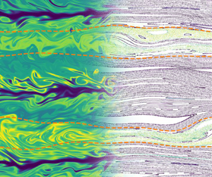
Figure 7. (a) Poincaré sections for the two cases, with tracers coloured by the computed correlation dimension  $d_C$ of their orbit. Invariant tori bounding the major chaotic regions are highlighted with an orange dashed line. (b) Direct numerical simulation snapshots of the PV $q+\beta y$. The colour $\ell _q$ is the time-averaged length of the level set contour of $q+\beta y$ which encircles the domain. The invariant tori are again shown with an orange dashed line. (c) Comparison of the time- and zonally averaged PV gradient $\bar {q}'(y) + \beta$ (blue) with the fraction of orbits which are chaotic $f_{chaotic}$ (orange, filled). The dashed black line shows the background PV gradient $\beta$.
The first measure of mixing considered is the temporally and zonally averaged PV gradient  $\bar {q}'(y) + \beta$. Friction and viscosity tend to push $\bar {q}'(y)$ towards zero, pushing the the PV gradient towards the background value of $\beta$. Meanwhile, turbulent mixing tends to push the PV gradient towards zero. Figure 7(c) shows the PV gradient compared against the fraction of orbits which are chaotic at some $y$ for cases 1 and 2. This fraction is computed by computing the average $y$ of the particles, binning them into equally sized bins based on this average $y$, then computing the fraction of particles whose orbits have $d_C \ge 1.5$.
In every region where there is a significant fraction of chaotic orbits, the PV gradient is pushed below the background  $\beta$, indicating a region of sustained turbulent mixing. Furthermore, in case 2 these chaotic regions and corresponding mixing regions are not in the centre of their respective broad westward flow regions. The particular combination of Rossby waves produces an asymmetry in the chaotic regions that matches the asymmetry in the observed turbulent mixing regions.
A second measure of mixing comes from the consideration that in two dimensions, enstrophy is typically understood to be anomalously dissipated by viscosity via the formation of small-scale structure (Boffetta & Ecke Reference Boffetta and Ecke2012). In real space, this small-scale structure can be formed by the chaotic advection of level set contours of the PV  $q+\beta y$. The contours are stretched in directions with non-zero Lyapunov exponent, creating small-scale meanders and increasing the overall length of the contour. Eventually, the meanders reach a small enough scale that viscosity acts to reconnect and smooth the contours, limiting the growth of their length. To quantify this process in the DNS, the contours of $q+\beta y$ which encircle the domain are identified, then their length is computed and time-averaged over all DNS snapshots $\ell _q$. For a pure zonal flow $\bar {q}(y)+\beta y$, the undisturbed PV contours would be lines of constant $y$ with the minimum possible length of $\ell _q = L =2{\rm \pi}$.
Shown in figure 7(b) is the PV  $q + \beta y$, coloured by $\ell _q$, for the DNS snapshot whose eigenmode amplitudes and phases were used to construct the Poincaré sections in figure 7(a). In both cases, all of the chaotic regions identified in the Poincaré sections correspond to a region of mixing identified in the DNS. These mixing regions only exist in the broad westward flow regions, and are bounded on either side by regions consisting of shorter, less disturbed PV contours. The bulged shapes of the mixing regions also line up well with the invariant tori bounding the corresponding chaotic regions.
Physically, this mixing process corresponds to the formation of elongated filaments of PV in chaotic ‘surf zones’. These chaotic regions occur in the absence of critical layers where  $u_{ph} = U(y)$, and are a result of Rossby waves which are standing in $y$. Observing the fate of these filaments in figure 1, some of these filamentary structures undergo reconnection to form isolated vortex patches. Cusps form in the PV contour at the point of reconnection. This is reminiscent of the vortex filamentation and ‘microbreaking’ process observed in Dritschel (Reference Dritschel1988) and Polvani & Plumb (Reference Polvani and Plumb1992), although here the breaking occurs in the ‘bulk’ rather than at sharp PV interfaces. Drawing a loose analogy with the overturning of stably stratified density layers by breaking gravity waves, this Rossby wave breaking process ultimately leads to an irreversible ‘overturning’ of a stably stratified PV gradient. Note that there also appears to be a breaking process occurring at the sharp PV interfaces corresponding to the eastward jets as well, although this is not captured by the Poincaré section analysis.
Together, these two measures of mixing provide strong evidence that localization of wave-induced chaos leads to a form of inhomogeneous PV mixing. This is broadly consistent with the results in for example Del-Castillo-Negrete & Morrison (Reference Del-Castillo-Negrete and Morrison1993) and Haynes et al. (Reference Haynes, Poet and Shuckburgh2007), which show that the Lagrangian flow induced by zonal flows plus a few waves will generally create regions of mixing separated by invariant-torus-like transport barriers. Note from figure 7(c) that the PV gradient is actually close to or above the background value of  $\beta$ in many of the regions where the invariant tori survive, not just in the immediate vicinity of the transport barriers at the centre of the eastward jets. Thus, these tori can act as semi-permeable transport barriers over regions of finite area in the fully developed turbulence.
4.3. Self-organization into coherent Rossby waves
The paradigm of inhomogeneous PV mixing leading to ‘potential vorticity staircases’ has been established as a way to understand how turbulence reinforces, rather than destroys, large-scale zonal structure (Baldwin et al. Reference Baldwin, Rhines, Huang and McIntyre2007; Dritschel & McIntyre Reference Dritschel and McIntyre2008). Here, the parameter  $L_{Rh}/L_{\varepsilon } = (U/\beta )^{1/2} / (\varepsilon /\beta )^{1/5}$ identified in Scott & Dritschel (Reference Scott and Dritschel2012) is $\approx 6.5$ for case 1 and $\approx 2.6$ for case 2, suggesting the staircase regime is relevant. Chaos in the Poincaré sections was found to be localized near zonal flow minima of broad jets with the strongest westward flow, i.e. in the direction of propagation for the Rossby waves. Since the net $y$ (meridional) PV flux leads to a net zonal acceleration in the ideal QG model by the Taylor identity, this mixing would then reinforce the amplitude of the strongest westward jets. Note that this method of transfer of energy to the zonal flows does not resemble either a local or a self-similar cascade. The PV perturbations at all scales, including the forcing scales, are exponentially stretched by the chaotic flows induced by the box-scale waves. Again, this is broadly consistent with the picture in for example Haynes et al. (Reference Haynes, Poet and Shuckburgh2007) linking the survival of invariant tori to jet formation in QG.
Now moving beyond a zonally averaged sense, one key consequence of the survival of most invariant tori is that the majority of flow energy can be understood as being organized into a temporally and zonally varying laminar flow. Here, the remnants of the invariant-torus-like LCSs which fill space in the DNS are the ‘laminae’ which organize the flow. Appealing to the near-integrability established earlier, an argument can be constructed for why these laminar flows predominantly organize into long-lived Rossby waves. This will show how the paradigm of inhomogeneous mixing can be extended to describe coherent flow formation in non-zonal and temporally non-stationary components of the flow.
Since the perturbed PV  $\hat {q}_0 + q_1$ for regular Rossby wave eigenmodes is an approximate integral of motion, the perturbed PV contours will nearly align with the surviving invariant tori. While these contours will not be mapped exactly back onto themselves by the Poincaré map, they will still be confined by neighbouring invariant tori. This suggests that superpositions of Rossby waves with PV perturbations primarily localized to non-chaotic regions will enjoy a form of long-time nonlinear stability under the Poincaré map, as their PV perturbations are approximately mapped back onto themselves after any number of iterations of the map.
This spatially localized stability is demonstrated in figure 8 for cases 1 and 2. In quiescent regions, contours initially aligned with the perturbed PV contours remain nearly unchanged after many iterations of the Poincaré map. The example contours shown in the figure for cases 1 and 2 have undergone 16 iterations of the Poincaré map. Meanwhile in the chaotic regions, perturbed PV contours are rapidly distorted. Two iterations of the Poincaré map in case 1 and four iterations in case 2 are sufficient to stretch the contours shown in the figure to approximately  $\ell _q$. Lyapunov exponents in the chaotic regions can be estimated from the contour stretching, with $\lambda \approx 0.048$ in case 1 and $\lambda \approx 0.018$ in case 2, which are both a little slower than the Poincaré map frequency $\varOmega _0/(2{\rm \pi} ) \approx 0.065$.

Figure 8. For (a) case 1 and (b) case 2, the left-hand part of each panel shows the image of a contour of the perturbed PV  $\hat {q}_0 + q_1$ under several iterations of the Poincaré map. Light orange shows the initial contour and dark orange shows the final contour. A different number of iterations are applied on each contour, as described in the text. The right-hand part of each panel shows the ‘enstrophy’ $\langle \tilde {q}^2_{coherent}\rangle$ carried by the coherent waves at each $y$. The area enclosed by the curve is coloured by the contour length $\ell _q$ corresponding to the amount of mixing at each corresponding $y$.
$y$.
These nearly-integrable superpositions of Rossby waves can be thought of as generalizations of exact solutions to the QG equations consisting of pure plane waves in the absence of a background flow. In the latter, contours of PV align exactly with invariant tori. Physically, fluid parcels supporting the waves on invariant tori experience completely reversible perturbations from the large-scale waves. After one period of the Poincaré map, the material curves corresponding to invariant tori return to their original shapes. This allows the waves to survive for much longer times than suggested by the simple estimate  $\tau _{nl}/\tau _{lin} \sim u_{wave}/ u_{ph}$.
In contrast, large-scale PV perturbations which induce non-wave-like flows would produce significant misalignment between the perturbed PV contours and the surviving invariant tori. Examples are non-resonant beat modes between Rossby waves, or hydrodynamic vortices. Under the action of the Poincaré map, either chaos from destroyed tori or frequency shear between neighbouring invariant tori would shear these perturbations to smaller scales. Since  $\psi \sim k^{-2} q$, this damps the induced flow perturbations, with laminar shear due to invariant tori resembling the Orr mechanism (Orr Reference Orr1907). Thus, non-wave-like flows are prevented from accumulating significant amounts of energy, leaving only the coherent wave component of the flow.
Combining the factors of (i) inhomogeneous mixing leading to PV staircases, (ii) near-integrability of the Rossby waves and (iii) damping of non-wave-like perturbations together suggest that large-scale flows will invariably organize into coherent Rossby waves on top of zonal flows. Note that although the mechanism for transferring energy to the waves is not specified here, work in Bakas & Ioannou (Reference Bakas and Ioannou2014) and Constantinou, Farrell & Ioannou (Reference Constantinou, Farrell and Ioannou2016) has established that, using the turbulence closure provided by stochastic structural stability theory, non-zonal perturbations can extract energy from small-scale fluctuations. This can be viewed as the small-scale stirring self-organizing into macroscopically coherent waves.
One piece of evidence supporting this picture of wave self-organization in the DNS is the observation that the most coherent waves tend to have PV perturbations localized to the regions of weakest turbulent mixing. As shown in figure 8, the zonally averaged squared magnitude of the PV perturbation  $\langle \tilde {q}^2_{coherent}\rangle := \int _{0}^{L_x} q^2_1 \,\mathrm {d}\kern 0.06em x$, where $q_1$ is the superposition of the coherent Rossby wave eigenmodes, is localized to regions where the $q$ contours are stretched the least. This mostly corresponds to the sharp eastward jets, although there also tend to be larger PV perturbations outside of the large-scale Rossby wave ‘surf zones’ than inside.
Referring back to figure 5, this PV localization of coherent waves is also consistent with the observed ‘interfacial’ character of the most energetic eigenmodes. This suggests a possible ‘selection rule’ for determining which of the eigenmodes will maintain large amplitude and coherence in the fully developed turbulence. For case 1, the wavenumber  $(k_x,k_y) = (1,1)$ of the most energetic eigenmode is the largest scale wave which can approximately align its maximum and minimum with the two sharp eastward jets. Similarly for case 2, the wavenumber $(k_x,k_y) = (1,3)$ of the most energetic eigenmode is the largest scale wave which can align its three maxima with the three sharp eastward jets. Meanwhile, waves with more of a ‘bulk’ character are unable to align their minima and maxima with the surviving invariant tori. Thus ‘bulk’ waves would experience stronger mixing, presumably reducing their amplitude and coherence.
5. Discussion and outlook
5.1. Open issues in the QG system
Several questions remain regarding the turbulent mixing observed in the DNS. Referring back to figure 6, although a majority of the non-zonal flow energy is captured in the large-scale Rossby waves, there are still a number of modes with significant amplitude which were not included in the Poincaré map. These modes typically did not show a strong enough coherent character over several cycles to justify approximation by purely periodic flows. While LCSs can be defined for finite-time and aperiodic flows (see e.g. Haller Reference Haller2015), it is not clear if there is a generalization of the KAM theorem to such a situation.
This issue also arises when attempting to generalize the arguments in § 4 to the finite deformation radius  $k_D > 0$ case, where the PV becomes $\hat {q} = \nabla ^2 \psi - k_D^2 \psi + \beta y$. While the manipulations in § 3 are also formally valid for the $k_D > 0$ case, it is generally observed that as $k_D$ is increased, the flows tend not to organize into large-scale coherent waves (Suhas & Sukhatme Reference Suhas and Sukhatme2015). One possible avenue for future work is to better characterize the perturbative behaviour of elliptic LCSs in finite-time and aperiodic settings. This would clarify if the concept of near-integrability can be applied to identify ‘laminar’ character in flows which are locally rather than globally organized.
Additionally, the kinematics of transport driven by the wave-induced Lagrangian flows are not well understood analytically. The zonal flow is non-monotonic, so the Poincaré map does not satisfy the usual twist criterion (Meiss Reference Meiss1992). The chaos observed in the Poincaré sections also occurs in the complete absence of first-order resonances, since  $u_{ph} < U(y)$ everywhere for the coherent waves. This distinguishes the picture of wave-driven transport in the QG system from the typical picture of wave-driven transport via overlapping wave–particle resonances in Vlasov turbulence (Chirikov Reference Chirikov1979). It would be interesting to study how much of the observed route to chaos phenomenology in systems such as the Chirikov standard map or standard non-twist map (Del-Castillo-Negrete & Morrison Reference Del-Castillo-Negrete and Morrison1993) carry over to this system. This would provide insight into how the chaotic regions form and change in response to changes in the wave amplitudes and phases.
While this work does not develop a quantitative model for the long-time large-scale flow evolution in the QG system, the relevance of coherent Rossby wave eigenmodes suggests some promising areas for development. The majority of the flow energy can be described by ‘zonal flows plus a few waves’, i.e. a mean zonal flow profile  $U(y)$, and a set of eigenmode amplitudes and reference phases $\{A_i, \varTheta _i\}$. Compared with the approach of discrete wave turbulence using Fourier modes (see e.g. L'vov & Nazarenko Reference L'vov and Nazarenko2010), the role of low-order wave–wave resonances is de-emphasized. Wave–mean flow interactions have an unmistakable influence on both the Rossby wave eigenfunctions and the small-scale turbulence statistics. The latter is best understood in a real-space Lagrangian picture.
The clear impact of the wave-induced flows on the turbulence statistics also suggests that purely ‘quasi-linear’ approaches, which discard all nonlinear interactions between non-zonal modes, do not account for all of the inhomogeneous mixing in the QG system. This effect has already been recognized in the development of more general filtered quasi-linear approaches, such as in Constantinou et al. (Reference Constantinou, Farrell and Ioannou2016) and Marston, Chini & Tobias (Reference Marston, Chini and Tobias2016). However, the influence of small-scale fluctuations on the zonal flows and coherent waves appears to be small, changing  $U(y)$ and $\{A_i, \varTheta _i\}$ slowly compared with the linear Rossby wave time scales. An intriguing possibility is if the time-scale separation arguments in Bouchet, Nardini & Tangarife (Reference Bouchet, Nardini and Tangarife2013) and Woillez & Bouchet (Reference Woillez and Bouchet2019) can be extended to allow the zonal flows and coherent waves to play the role of ‘slow’ variables. This would represent a significant simplification compared to the general filtered quasi-linear approach, as the dominant effect of the interaction between zonal modes and near-zonal modes is to organize the near-zonal modes into eigenmodes.
5.2. Integrability beyond QG
Looking beyond the simple prototypical equations used in this work, waves with a strong linear character have been observed in turbulent settings in more complex and realistic flows. One example is shallow water turbulence in the equatorial region, where the signature of linear waves has been seen both in simulations (Garfinkel et al. Reference Garfinkel, Shamir, Fouxon and Paldor2021; Schröttle et al. Reference Schröttle, Suhas, Harnik and Sukhatme2022) and in observational data (Wheeler & Kiladis Reference Wheeler and Kiladis1999). Another example is the coexistence of internal gravity waves with turbulent balanced motions in the ocean, which has also been seen in idealized numerical simulations (Thomas & Yamada Reference Thomas and Yamada2019; Thomas & Daniel Reference Thomas and Daniel2020), global-scale ocean models (Richman et al. Reference Richman, Arbic, Shriver, Metzger and Wallcraft2012; Torres et al. Reference Torres, Klein, Menemenlis, Qiu, Su, Wang, Chen and Fu2018) and in observational data (Rocha et al. Reference Rocha, Chereskin, Gille and Menemenlis2016; Lien & Sanford Reference Lien and Sanford2019). Thus, it is interesting to ask if analogues of the results in §§ 3 and 4 hold in more complex, realistic flows.
The Rossby wave self-organization principle proposed in this work relied on three key ingredients: (i) the existence of enough materially conserved scalar invariants to guarantee Liouville integrability, i.e. a ‘laminar’ phase-space flow; (ii) KAM theory, which characterized the persistence of the invariant tori ‘laminae’ under perturbations; and (iii) the PV inversion equation (2.2), which allowed the near-integrability conditions to be written into a form coinciding with the linearized evolution equations. Note that points (i) and (ii) are more ‘kinematic’, in the sense that they would describe the motion of any passive scalar advected by the flow. Meanwhile, point (iii) is more ‘dynamical’, in the sense that it links the passive scalar advection back to the fully self-consistent flow.
First considering point (i), the concept of PV conservation persists in a broad range of fluid and plasma systems (see e.g. Müller Reference Müller1995; Gurcan & Diamond Reference Gürcan and Diamond2015). Many fluid and plasma models of interest also conserve other scalar material invariants, such as specific entropy or related notions of potential temperature and density. Furthermore, recent work has extended notions of Liouville integrability to generic dynamical systems (Bogoyavlenskij Reference Bogoyavlenskij1998; Zung Reference Zung2016). This suggests the possibility of extending the Lagrangian integrability results in § 3 to more complex and realistic flow models, such as the shallow water or Boussinesq equations. In the absence of forcing and dissipation, these systems typically conserve some form of PV, with the latter also typically conserving some form of buoyancy or potential density.
Now considering point (ii), intuitively when a fluid or plasma flow conserves a scalar material invariant  $f$, the level sets of $f$ will generally form co-dimension one material surfaces (i.e. curves in two dimensions, surfaces in three dimensions) through which fluid parcels do not pass transversally. If the dominant motions of these material surfaces are ‘reversible’, then the surfaces could correspond to invariant-torus-like LCSs. Recent extensions of KAM theory to measure-preserving dynamical systems (Xia Reference Xia1992) may shed light on the conditions necessary for these transport barriers to survive in fully developed turbulent flows. However for point (iii), in most fluid and plasma systems the velocity field is typically not determined by scalar material invariants like the PV or specific entropy alone.
Together, these points suggest the ‘kinematic’ arguments of §§ 3 and 4 regarding the presence of invariant-torus-like LCSs in fully developed turbulent flows may directly generalize to more complex flow systems. However, the ‘dynamical’ arguments regarding the self-organization of flows into waves do not appear to have a direct route for generalization. The development of these arguments in detail is left for future work.
Finally, one other key aspect which is missing from this work is the presence of linear instabilities driven by gradients of quantities such as temperature or density, such as baroclinic instabilities or drift wave instabilities. In systems with marginally unstable gradients, found for example in fusion plasmas (Diamond & Hahm Reference Diamond and Hahm1995), the interaction between zonal flows and turbulent mixing of driving gradients can lead to non-trivial mesoscale behaviour such as avalanching (Dif-Pradalier et al. Reference Dif-Pradalier, Hornung, Garbet, Ghendrih, Grandgirard, Latu and Sarazin2017). Future work can also explore how transitions to chaos in Lagrangian flows interplay with linear instability dynamics.
6. Summary
In summary, this work proposes that the dynamics of large-scale coherent flows in QG turbulence can be understood as ‘nearly-integrable Rossby waves past the breaking point in zonally dominated turbulence’. The nearly steady zonal flow background acts as a waveguide supporting Rossby wave eigenmodes which are standing in  $y$ and propagating in $x$. The largest-scale modes accumulate a significant fraction of the flow energy yet retain a strong linear coherent character.
An integrability result on Lagrangian flow in QG was given, and regular Rossby wave eigenmodes were characterized as minimally perturbing to this integrability. Chaos in the wave-induced Lagrangian flow was identified using a Poincaré map, demonstrating that localization of chaos and subsequent ‘wave breaking’ was linked to the observed inhomogeneous PV mixing in the DNS. This inhomogeneous mixing was linked to a self-organization principle for the large-scale flows, suggesting that surviving invariant tori organize the observed zonal jets plus Rossby waves into a single zonally and temporally varying laminar flow.
More broadly, this Lagrangian picture of turbulent flow organization emphasizes the importance of considering the combined nonlinear effect of both zonal and non-zonal modes in the QG system. In the staircase regime when both zonal flows and Rossby waves are strong, the effects of wave–mean flow interactions were emphasized, whereas the roles of low-order wave–wave resonances were de-emphasized. Finally, it was discussed how there may be opportunities to extend the arguments in this work to more complex and realistic flow systems.
Acknowledgements
T. Grafke, J. Shatah and E. Vanden-Eijnden are thanked for fruitful discussions with the author, and several anonymous reviewers are thanked for their constructive commentary and insight.
Funding
This research was supported by the Simons Collaboration Grant on Wave Turbulence, grant no. 617006.
Declaration of interests
The author reports no conflict of interest.
Data availability statement
The codes used in this study are openly available in GitHub at https://github.com/Maplenormandy/qg-edgeofchaos.


 Open access