


1. Introduction
After more than a century of scientific research efforts, the flow around bluff bodies is still an open problem. Despite the accumulation of a huge amount of empirical data and of descriptive knowledge, the progress towards a sufficiently general and unified solution of the basic problem has been slow. In fact, the advances of the theoretical framework from the pioneering works of Kirchhoff (Reference Kirchhoff1869), von Kármán (Reference von Kármán1954) and Roshko (Reference Roshko1955) are still limited. Indeed, arriving at a complete theory still requires the understanding of the interplay between the different phenomena composing the flow. The strongly inhomogeneous and anisotropic character of the overall flow is related with the non-local and nonlinear interactions between these flow mechanisms that challenges for a rational understanding. In fact, a theoretical model able to unify these interacting phenomena is still lacking. In this context, the access to high-fidelity data is deemed of fundamental importance, as these can be considered as a fruitful source for ideas, can be used to confirm or extend the validity of theories and, in some cases, can give rise to new questions. This is the approach pursued in the present work where high-fidelity numerical simulations of the flow around a rectangular cylinder with aspect ratio 5 are performed at increasing Reynolds numbers. The main aim is to address the detailed physics of the different phenomena composing the flow and to assess their role on the overall behaviour of the flow, thus allowing us to provide a sufficiently general and self-contained description of the basic problem.
The case under scrutiny is the object of an international initiative known as BARC (Benchmark on the Aerodynamics of a Rectangular 5 : 1 Cylinder; http://www.aniv-iawe.org/barc). Several experimental and numerical studies have been conducted on this benchmark and, as shown in the review by Bruno, Salvetti & Ricciardelli (Reference Bruno, Salvetti and Ricciardelli2014), a significant dispersion of the results is observed, thus highlighting how challenging is the correct description of the fundamental features of the flow. From a numerical point of view this issue can be faced by adopting a sufficiently high spatial resolution to avoid the use of turbulence models. Cimarelli, Leonforte & Angeli (Reference Cimarelli, Leonforte and Angeli2018b) were the first to perform a direct numerical simulation (DNS) of such flow configuration. The value of the Reynolds number based on the body thickness and the freestream velocity was  $Re=3000$. This value was found to be large enough to study the main self-sustaining features of turbulence in the separating and reattaching flow but one decade smaller than that expected to characterise the high-Reynolds-number regime of the flow. Later, Chiarini & Quadrio (Reference Chiarini and Quadrio2021) replicated the work by performing an additional DNS at the same Reynolds number to address the detailed features of production, transport and dissipation of Reynolds stresses of relevance for turbulence closures. Finally, Corsini et al. (Reference Corsini, Angeli, Stalio, Chibbaro and Cimarelli2022) performed a third DNS, again at $Re = 3000$, to study the effects of spatial resolution and numerical schemes on the main statistical features of the flow. In the present work we extend the Reynolds number achieved by high-fidelity simulations significantly by performing DNS at three Reynolds numbers, $Re=3000$, $8000$ and $14{\,}000$. The behaviour of turbulence and of the main flow unsteadiness by increasing $Re$ towards the high-Reynolds-number regime is addressed. The mechanisms of passive scalar transport at the basis of the values of heat exchange in bluff bodies are also addressed for the first time.
The work is organised as follows. The numerical method and the flow settings are described in § 2. The main flow features are introduced through the analysis of the instantaneous flow pattern in § 3. The mean flow statistics are addressed in §§ 4 and 5. The turbulent phenomena and the entrainment mechanisms characterising the shear layer detaching from the sharp leading edge and the wake are studied in §§ 6 and 7. Finally, the main flow unsteadiness are analysed in § 7. The work is closed by a final discussion in § 9 and by the validation of the numerical database in Appendix A.
2. Numerical method and flow setting
Three DNSs of the flow around a rectangular cylinder with aspect ratio  $5$ are performed by varying the Reynolds number and considering the transport and mixing of a passive scalar. The system of equations solved is
 \begin{equation}
\left. \begin{array}{@{}l@{}} \displaystyle \dfrac{\partial
u_i}{\partial x_i} = 0, \\
\displaystyle \dfrac{\partial u_i}{\partial t} + \dfrac{\partial u_i u_j}{\partial x_j} =
\displaystyle -\dfrac{\partial p}{\partial x_i} +
\dfrac{1}{Re} \dfrac{\partial^2 u_i}{\partial x_j \partial x_j}, \\
\displaystyle \dfrac{\partial \theta}{\partial t}
+ \dfrac{\partial u_i \theta}{\partial x_i} = \displaystyle
\dfrac{1}{Re{\textit{Pr}}} \dfrac{\partial^2
\theta}{\partial x_i \partial x_i}, \end{array}\right\}
\end{equation}
\begin{equation}
\left. \begin{array}{@{}l@{}} \displaystyle \dfrac{\partial
u_i}{\partial x_i} = 0, \\
\displaystyle \dfrac{\partial u_i}{\partial t} + \dfrac{\partial u_i u_j}{\partial x_j} =
\displaystyle -\dfrac{\partial p}{\partial x_i} +
\dfrac{1}{Re} \dfrac{\partial^2 u_i}{\partial x_j \partial x_j}, \\
\displaystyle \dfrac{\partial \theta}{\partial t}
+ \dfrac{\partial u_i \theta}{\partial x_i} = \displaystyle
\dfrac{1}{Re{\textit{Pr}}} \dfrac{\partial^2
\theta}{\partial x_i \partial x_i}, \end{array}\right\}
\end{equation}
where  $(x_{1}, x_{2}, x_{3}) = (x, y, z)$ are the spatial coordinates in the streamwise, vertical and spanwise direction, $(u_{1}, u_{2}, u_{3}) = (u, v, w)$ are the corresponding components of the velocity field, $p$ is pressure and $\theta$ is the scalar field. The adopted reference frame is centered at the upper leading edge of the rectangular cylinder, see figure 1. The thickness of the rectangular cylinder $D$, the freestream velocity $U_0$ and the temperature difference between the cylinder surface and the freestream $\Delta \theta = \theta _w - \theta _{0}$ are used for non-dimensionalisation of the above equations. Accordingly, the Reynolds number is defined as $Re = U_0 D / \nu$, with $\nu$ the kinematic viscosity, whereas ${\textit {Pr}} = \nu / \alpha$ denotes the Prandtl number, having in mind temperature as the passive scalar, with $\alpha$ the scalar diffusivity. Equation (2.1) are solved by imposing the freestream velocity $U_{0}$ at the inlet. The outlet boundary condition consists of a homogeneous Dirichlet condition for the pressure and a homogeneous Neumann condition for the velocity. These same boundary conditions are imposed in the vertical direction whereas the no-slip condition is imposed at the cylinder surface. Concerning the passive scalar field, the inlet and the cylinder surface are held at fixed values $\theta _0 = 0$ and $\theta _w=1$, respectively. A homogeneous Neumann condition is applied at the outlet and in the vertical directions. Finally, periodicity is enforced along the spanwise direction for both the velocity and the scalar fields.

Figure 1. Flow configuration and computational domain.
The simulations have been performed using the open-source code Nek5000, developed by Fischer, Lottes & Kerkemeier (Reference Fischer, Lottes and Kerkemeier2008) and based on the high-order spectral element method proposed by Patera (Reference Patera1984). Velocity variables are expanded within the numerical elements in terms of polynomials of order  $N$ that are collocated within each element following the Gauss–Lobatto–Legendre (GLL) distribution. On the other hand, a staggered-grid approach based on the use of pressure polynomials of order $N-2$ is employed to avoid spurious pressure modes, following the so-called $P_{N}-P_{N-2}$ formulation. Time advancement is performed by means of an implicit scheme consisting of a third-order backward differentiation scheme (BDF3) used in combination with a third-order extrapolation scheme (EXT3) for the explicit treatment of the convective term. In the DNS at highest $Re$, the same method but second-order accurate in time is used. De-aliasing is performed by over-integration of the convective term by a factor of 3/2 in each direction. For stabilisation, a filtering procedure based on a low-pass explicit filter built in modal space with a cut-off mode of $N-1$ and a weight of $0.02$ is applied (Fischer & Mullen Reference Fischer and Mullen2001).
The computational domain dimensions normalised by the body thickness are  $(L_x, L_y, L_z) = (80, 31, 5)$ and the rectangular cylinder is placed $20$ length scales downstream from the inlet, see figure 1. The investigated Reynolds numbers are ${Re = 3000}$, $8000$, and 14 000, whereas the Prandtl number is set to ${\textit {Pr}} = 0.71$. Spatial discretisation is performed by using a structured mesh composed by hexahedral spectral elements of order $N=7$, corresponding to a seventh order of accuracy. The total degrees of freedom per time step and per unknown for the flow case at $Re = 3000$ are almost $178$ million, and increase up to over $3$ billion at $Re = 14{\,}000$, see table 1. Although the spectral elements are uniformly distributed along the spanwise direction, the mesh is refined through geometric progressions along the vertical direction by approaching the walls and along the streamwise direction by moving towards the rectangle edges. Accordingly, the minimum grid spacing $(\Delta x_{min}, \Delta y_{min})$ is achieved at the leading-edge corner and the corresponding values are reported in table 1, including also the number of degrees of freedom adopted on the horizontal surface of the rectangular cylinder. As reported in Corsini et al. (Reference Corsini, Angeli, Stalio, Chibbaro and Cimarelli2022), the occurrence of strongly inhomogeneous phenomena in the flow around the rectangular cylinder requires different spatial discretisation criteria to be satisfied such as those based on the Kolmogorov length for the free flow and on the friction units for the boundary layers. The details of the computational grids are summarised in table 1. The time step is kept fixed during the simulation to ensure that the condition $\mathrm {CFL} < 0.5$ is satisfied everywhere, resulting in $\Delta t = 5.5 \times 10^{-4}$, $3.0 \times 10^{-4}$ and $2.6 \times 10^{-4}$ for the flow cases at $Re = 3000$, $8000$ and 14 000, respectively.
Table 1. Numerical details. Here  $n_x$, $n_y$ and $n_z$ are the degrees of freedom adopted in the region above the cylinder; $\Delta x, \Delta y, \Delta z$ are computed as the distance between $N+1$ uniformly spaced points within a spectral element, except to the near-wall resolution $\Delta y_w$ which is expressed as the wall distance of the second GLL point. The superscript $+$ indicates friction units and $\eta$ denotes the Kolmogorov scale.

Statistics are computed by taking advantage of the statistical steadiness and of the statistical homogeneity in the spanwise direction of the flow. Hence, a spanwise average is performed together with a temporal average over a collection of at least  $51$ three-dimensional fields gathered at equal time intervals $\Delta T = 5$ and after the statistically steady conditions are reached. Furthermore, the flow exhibits a statistical symmetry in the vertical direction about the $xz$ mid-plane that is also used for improving the statistical convergence. The quality of the database in terms of both spatial discretisation and statistical convergence is reported in Appendix A where a validation is also performed through a comparison with experimental data. In the following, the Reynolds decomposition of the flow in a mean and fluctuating field is adopted and indicated using the customary nomenclature, i.e. $u_i = U_i + u_i'$ and $p = P + p'$. If not stated specifically, variables are presented as dimensionless by using $D$ for lengths, $U_0$ for velocities, $D/U_0$ for times and $\Delta \theta$ for temperatures.
3. Instantaneous flow topology
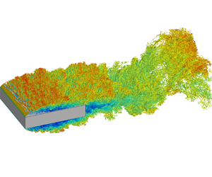
We start the analysis by addressing the effect of the Reynolds number on the flow topology visualised by means of the so-called  $\lambda _2$ criterion proposed by Jeong & Hussain (Reference Jeong and Hussain1995) and reported in figures 2 and 3. We take advantage of these flow visualisations to introduce and describe the main features of the flow. The picture is as follows.

Figure 2. Instantaneous three-dimensional views of the flow cases at  $Re = 3000$ (a,b), $Re = 8000$ (c,d) and $Re = 14\ 000$ (e, f). The plots report isosurfaces coloured with streamwise velocity of $\lambda _{2} = -2$, $-4$ and $-5$, respectively, from the lowest to the highest $Re$. The perspective view is reported in the left column and the lateral view in the right column.

Figure 3. Instantaneous three-dimensional top views of the flow cases at  $Re = 3000$ (a,b), $Re = 8000$ (c,d) and $Re = 14{\,}000$ (e, f). The plots report isosurfaces coloured with streamwise velocity of $\lambda _{2} = -2$, $-4$ and $-5$, respectively, from the lowest to the highest $Re$. To highlight the vortical structures in the reverse flow region, only isosurfaces with negative streamwise velocity, $u<-0.2$, are shown in the right column.
By impinging to the front of the rectangular cylinder, the incoming flow creates two ascending/descending laminar boundary layers. By reaching the sharp leading edge of the cylinder, these boundary layers detach thus forming two shear layers that are initially laminar as highlighted by the flat shape of the isosurface of  $\lambda _2$, see the left panels of figures 2 and 3. The separated shear layer is inviscidly unstable (Dovgal, Kozlov & Michalke Reference Dovgal, Kozlov and Michalke1994) and easily undergoes transition to turbulence. As expected, the transitional processes are found to occur more rapidly by increasing $Re$, see the reduced size of the flat isosurface of $\lambda _2$. At the early stages of the transition process, almost two-dimensional spanwise rolls are initiated due to the Kelvin–Helmholtz instability. As apparent from the perspective and top views shown in the left panels of figures 2 and 3, the diameter of these rolls significantly reduces by increasing $Re$ and their spanwise distribution becomes progressively more irregular. As shown in Cimarelli et al. (Reference Cimarelli, Leonforte and Angeli2018b), the combined presence of disturbances and strong mean shear leads to a distortion of these spanwise rolls thus forming hairpin-like vortical structures and quasi-streamwise vortices, see also Kiya & Sasaki (Reference Kiya and Sasaki1985), Hourigan, Thompson & Tan (Reference Hourigan, Thompson and Tan2001), Yang (Reference Yang2012) and Chiarini et al. (Reference Chiarini, Gatti, Cimarelli and Quadrio2022).
By moving downstream, the coherent structures populating the shear layer eventually break down into small irregular vortices thus leading to a fully turbulent regime. By increasing  $Re$ this process occurs in a shorter distance thus making the flow pattern more irregular and less coherent. As a result, the flow appears to be fully turbulent from the very beginning of the cylinder at high $Re$. This scenario is quantitatively confirmed by the one-dimensional wavenumber spectra $E(k_z)$ shown in figure 4(a). Here,
 \begin{equation} E(k_z) = \tfrac{1}{2} ( \langle \hat{u}_{z} \hat{u}_{z}^* \rangle + \langle \hat{v}_{z} \hat{v}_{z}^* \rangle + \langle \hat{w}_{z} \hat{w}_{z}^*\rangle ), \end{equation}
where  $\widehat {\cdot }_z$ denotes the Fourier transform in the periodic spanwise direction, $k_z$ is the spanwise wavenumber and the superscript $*$ denotes the complex conjugate. As expected, the fully developed region exhibits a wider spectrum of turbulent scales by increasing $Re$ while almost preserving the same behaviour at the large energy-containing scales. This generation of progressively smaller scales allows for a net separation of scales for the highest Reynolds number and, hence, for the realisation of a clear inertial subrange of scales where the classical $k^{-5/3}$ scaling more than one decade wide holds.

Figure 4. One-dimensional wavenumber spectra of the turbulent kinetic energy  $E(k_z)$ evaluated in (a) the primary vortex shedding region at position $(3.90, 0.40)$ and in (b) the attached reverse boundary layer at position $(3, 0.07)$: dotted line, $Re = 3000$; dashed line, $Re = 8000$; full line, $Re = 14{\,}000$. The red line displays the $-5/3$ slope.
These turbulent structures are transported by a very large-scale motion associated with the main flow separation. As a consequence, some of these are convected down towards the plate wall and follow a recirculating path (hereafter called primary vortex) whereas others are shed in the wake. The former, after impinging to the downstream part of the plate, give rise to a reverse boundary layer, see the right panels of figure 3. As shown in § 5, this reverse boundary layer undergoes an adverse pressure gradient that causes its separation thus forming a counter-rotating secondary vortex within the primary vortex. By increasing the Reynolds number, the reverse boundary layer is found to be populated by a wider range of turbulent structures, see again the right panels of figure 3. As better shown in § 5, this feature allows the reverse boundary layer to counter the adverse pressure gradient over longer distances thus pushing the secondary vortex towards the front of the cylinder and reducing its size. The fully turbulent feature of the reverse boundary layer for the highest Reynolds numbers is quantitatively verified by the one-dimensional spectra  $E(k_z)$ shown in figure 4(b). A wider spectrum of turbulent scales is found to populate the reverse boundary layer by increasing $Re$. In contrast to the free-flow region shown in figure 4(a), a less evident inertial subrange of scales is generated due to the strong inhomogeneous character of the boundary layer with respect to the free flow.
Finally, the flow structures that are shed from the primary vortex together with those shed from the forward boundary layer are convected in the wake where eventually undergo a last very large-scale motion related to the flow separation at the trailing edge of the rectangular cylinder. As shown by the lateral views of figure 2, this motion consists in a very large-scale flow oscillation induced by spanwise vortices reminiscent of the von Kármán instability typical of bluff bodies (Chiarini et al. Reference Chiarini, Gatti, Cimarelli and Quadrio2022). This large-scale unsteadiness appears to be almost unaltered by varying the Reynolds number. In fact, the main difference is the number of progressively smaller structures advected by these large-scale motions by increasing  $Re$.
$Re$.
4. Aerodynamic forces and heat transfer
In wind engineering applications, the aerodynamic and heat exchange coefficients are useful for the prediction of wind loads on buildings and structures and for their thermal efficiency. Global quantities such as the drag coefficient  $C_D$ and the heat transfer coefficient $C_H$ (also known as the Stanton number) are expected to reach asymptotic values for sufficiently high Reynolds numbers (Frisch Reference Frisch1995), see their definitions reported in Appendix B. In the present section we address their behaviour.
As shown in figure 5(a), the drag coefficient  $C_D$ shows an increase with $Re$ thus suggesting that the asymptotic regime is still not reached. Hence, our data, even at the highest Reynolds numbers, do not allow us to infer about the exact asymptotic value of $C_D$. In this respect, it is worth noting that also literature results from experiments at higher Reynolds numbers do not allow to solve this issue being characterised by a large scatter, see again figure 5(a) where some of them are reported. As shown in table 2, the observed increase in drag is driven by an increase in the form drag $C_{D_p}$ combined with a decrease of thrust induced by friction in the reverse boundary layer $C_{D_f} < 0$. The increase of the former is essentially due to a decrease in the base pressure of the wake that, in turn, is associated with a slight elongation of the primary vortex with $Re$ as shown in § 5. In particular, we measure that the local minimum of pressure within the wake vortex decreases from $p_{wv} = -0.142$ to $-0.163$ with $Re$. On the other hand, the observed decrease in thrust with the Reynolds number is essentially induced by a decrease in the friction coefficient $c_f$ with $Re$, again as shown in § 5. This decrease overcome the effect of a slightly longer flow recirculation that in contrast would lead to an increase in thrust with $Re$.
$Re$.

Figure 5. Behaviour of the drag coefficient  $C_D$ (a), of the Stanton number $C_H$ (b), of the Nusselt number $Nu$ (c) and of the lift coefficient fluctuations $C_{L_{rms}}$ (d) as a function of $Re$ for the present simulations and other works from the literature: $\bigcirc$, present data; $\square$, DNS data from Cimarelli, Leonforte & Angeli (Reference Cimarelli, Leonforte and Angeli2018a); $\bigtriangleup$, DNS data from Chiarini & Quadrio (Reference Chiarini and Quadrio2021); $+$, wind tunnel (WT) data from Schewe (Reference Schewe2013); $\ast$, WT data from Mannini et al. (Reference Mannini, Marra, Pigolotti and Bartoli2018); $\blacksquare$, WT data from Wu et al. (Reference Wu, Li, Li and Zhang2020); and $\blacklozenge$, water channel (WC) data from Kumahor & Tachie (Reference Kumahor and Tachie2022).
Table 2. Summary of the measured aerodynamic and heat coefficients.

In analogy with the momentum transfer measured with the drag coefficient  $C_D$, also the heat transfer measured with the Stanton number $C_H$ is found to have not reached an asymptotic state. As shown in figure 5(b), the dimensionless heat transfer $C_H$ is found to decrease with $Re$. The Stanton number is the counterpart of the drag coefficient and measures the ratio between the heat transferred and the thermal capacity of the undisturbed flow. It is related with the Nusselt number, $C_H = Nu / (Pr Re)$, that measures the ratio of convective to conductive heat transfer. Hence, the Nusselt number is expected to monotonically increases with $Re$ and does not have an asymptotic value. As shown in figure 5(c), the scaling followed by the Nusselt number is
 \begin{equation} Nu \sim Re^{2/3}. \end{equation}
This scaling agrees with the transitional power law reported in Ota & Kon (Reference Ota and Kon1974) but it is slower than the asymptotic linear scaling  $Nu \sim Re$ that would lead to a constant $C_H$.
In closing this section, let us address the behaviour of the lift coefficient  $C_L$. For the symmetry of the flow, the lift coefficient is null but its fluctuations are not. The intensity of fluctuations of lift are of relevance for several applications but is found to be particularly sensitive to the numerical and experimental set-up, as evidenced by the large spread of results reported in the literature (Bruno et al. Reference Bruno, Salvetti and Ricciardelli2014). As shown in figure 5(d), $C_{L_{rms}}$ is found to increase with $Re$. Forthcoming analysis reported in § 8 demonstrate that such an increase is essentially related with a strengthen of the vortex shedding phenomena. Indeed, the fluctuations of lift are generated by the instantaneous imbalance of pressure between the two sides of the cylinder induced by vortex shedding that alternately shrinks and enlarges the separation bubble at the top and bottom sides of the body. Accordingly, the frequency spectrum of lift (not shown) shows a well-defined peak at the frequency of vortex shedding.
5. Mean flow statistics
5.1. Velocity and pressure fields
In the present section the single-point statistics of the velocity and pressure fields are reported. By considering first the mean velocity field, it is possible to characterise the previously mentioned three main flow recirculations. As shown in the left panels of figure 6, the mean flow circulation related to the primary vortex (green streamlines) exhibits a significant Reynolds number dependence. It mainly consists in a shaping of the mean flow pattern rather than in a sizing of its dimensions. Indeed, the primary vortex streamwise length measured with the reattachment length  $x_r$ exhibits only a slightly increase with $Re$, see table 3 and the behaviour of the friction coefficient in figure 7(a). On the other hand, the thickness of the primary vortex results to be almost unchanged with $Re$.
$Re$.

Figure 6. Mean flow fields for the flow cases at  $Re=3000$ (a,b), $8000$ (c,d) and 14 000 (e, f). The left panels report the isocontours of the stream function. The green lines show the primary vortex, the red lines the secondary vortex and the black lines the wake vortex. The right panels display the mean pressure field. For statistical symmetry reasons, only the top half of the flow is shown.
Table 3. Details of the mean flow configuration;  $x_r$ is the reattachment length; $(x_c, y_c )$ are the coordinates of the vortex center; $x_s$ and $x_e$ indicate the coordinates of the start and end, respectively, of the secondary and wake vortices.


Figure 7. Behaviour of the skin friction coefficient (a), of the Nusselt number (b), of the pressure coefficient (c) and of its standard deviation (d): dotted line,  $Re = 3000$; dashed line, $Re = 8000$; and full line, $Re = 14{\,}000$.
The shaping effect consists in a significant upstream shift of the centre of rotation of the flow circulation that leads to a significantly different flow pattern, see again the left panels of figure 6. The behaviour of the centre of rotation  $\boldsymbol {x}_c = (x_c, y_c)$ as a function of $Re$ is presented in table 3. The vertical location is almost Reynolds independent, $y_c \approx 0.33$, whereas a significant upstream shift is observed when comparing its streamwise location at $Re = 3000$ with that at $Re = 8000$ and 14 000, see again table 3.
We argue that the upstream shift of the centre of rotation of the primary vortex is connected with the Reynolds number behaviour of the reverse boundary layer and of its separation, the secondary vortex highlighted with red streamlines in the left panels of figure 6. As shown in the right panels of figure 6, from the flow impingement at  $x_r$, the reverse boundary layer accelerates first towards the front of the cylinder due to a favourable pressure gradient. This gradient is induced by the near-wall footprint of the low pressure levels related to the centre of rotation of the primary vortex, see the behaviour of the pressure coefficient shown in figure 7(c). In contrast, by moving further towards the front of the cylinder, the reverse boundary layer experiences an adverse pressure gradient, decelerates and eventually detaches thus forming the secondary vortex (Cimarelli et al. Reference Cimarelli, Leonforte and Angeli2018b), see again the right panels of figure 6 and the pressure coefficient shown in figure 7(c). By increasing the Reynolds number the reverse boundary layer is populated by a wider spectrum of turbulent fluctuations. As a result, it turns out to be able to counter the adverse pressure gradient more efficiently for increasing $Re$ thus leading to a wider region of the plate where the reverse boundary layer remains attached to the wall, see the extension of the region of negative friction coefficient shown in figure 7(a). As a consequence, its separation, the secondary vortex, is found to significantly move upstream and to shrink by increasing the Reynolds number, see again the left panels of figure 6 and the corresponding positive region of friction coefficient in figure 7(a). As indicated quantitatively in table 3 by $x_c^{SV}$, this trend does not appear to saturate, $x_c^{SV} = 1.57$, $0.38$ and $0.26$ by increasing $Re$, thus suggesting the possibility of a disappearance of the secondary vortex at higher Reynolds numbers.
This upstream shift of the secondary vortex is here conjectured to be at the basis of the observed upstream shift of the centre of rotation of the primary vortex. Indeed, the upstream behaviour of the mean flow paths of the primary vortex are increasingly free from the fluid dynamic obstacle imposed by the secondary vortex. This occurrence allows for the development of a more symmetric primary vortex flow circulation and, hence, for the upstream shift of its centre of rotation towards central streamwise locations,  $x_c \sim x_r/2$. It is worth noting that this upstream shift of the centre of rotation of the primary vortex is in turn related to an upstream shift of the associated low-pressure region, see again the right panels of figure 6. This phenomenon further promotes the stability of the reverse boundary layer by extending the region of favourable pressure gradient. In summary, the higher turbulence levels in the reverse boundary layer with $Re$ lead to a shift towards the front of the plate of both the secondary vortex and of the primary vortex low-pressure levels with the latter further promoting the stability of the reverse boundary layer itself thus forming a self-amplifying mechanism.
We consider now the behaviour of the flow in the wake. Together with the primary vortex, the wake of the flow is the site of very large unsteadinesses in the form of shedding of very large vortical motions, see Chiarini et al. (Reference Chiarini, Gatti, Cimarelli and Quadrio2022) and § 3. The shape of the flow recirculation in the wake is reported with black streamlines in the left panels of figure 6. In contrast to the primary vortex recirculation, the size of the wake vortex is found to slightly decrease with Reynolds. In particular, as reported in table 3, the extension of the wake vortex moves from  $x_e^{WV} = 5.9$ to $5.8$ from the lowest to the highest Reynolds number. An upstream shift of its centre of rotation is also observed, $x_c^{WV} = 5.38$ at $Re = 3000$ and $x_c^{WV} = 5.3$ at $Re = 14{\,}000$. It is important to highlight that the values of pressure associated with the wake vortex decrease by increasing $Re$. As shown in § 4, this phenomenon is the main responsible for the observed increase in the drag coefficient with $Re$. We argue that the decrease in the wake vortex pressure can be attributed to two distinct reasons. The first is the slight downstream shift of the reattachment length of the primary vortex with $Re$. Indeed, the increasing length of the primary vortex leads to an elongation of the related low pressure levels towards the trailing edge thus reducing the base pressure, see again the right panels of figure 6. The second reason is in contrast related with the observed upstream shift of the centre of rotation of the primary vortex with $Re$. A consequence of this upstream shift is a more symmetric pattern taken by the mean recirculating flow that conforms with lower level of curvature of the mean streamlines in the downstream part of the primary vortex, see left panels of figure 6. Such reduction in curvature of the mean flow can be related to a lower pressure recovery ( $\partial p / \partial n \sim 1/R$ in laminar conditions, with $n$ the streamline normal direction and $R$ the curvature radius). In conclusion, we conjecture that the combination of a slightly longer primary vortex with lower streamline curvature by increasing $Re$ is at the basis of a weaker pressure recovery thus leading to lower values of base pressure in the wake, see also the behaviour of the pressure coefficient shown in figure 7(c).
To close this section, we address the behaviour of the pressure fluctuations at the body surface. This quantity is of relevance in wind engineering, being responsible for the so-called wind loads in civil applications. As shown in figure 7(d), the standard deviation of the pressure coefficient exhibits a distributed increase by augmenting the Reynolds number. Accordingly, the shape of the distribution appears to be almost unaltered especially considering the two highest  $Re$. Indeed, it is recognised that the peak of pressure fluctuations is located in the reattachment region of the primary vortex (Lunghi et al. Reference Lunghi, Pasqualetto, Rocchio, Mariotti and Salvetti2022). There, the periodic shedding of large-scale structures from the primary vortex leads to a continuous enlargement and shrinking of its size. Hence, a periodic upstream and downstream oscillation around the mean reattachment position of the related low pressure levels occurs (Cimarelli et al. Reference Cimarelli, Leonforte and Angeli2018b) thus leading to a peak value of the wall pressure fluctuations. The reattachment length of the primary vortex is almost unchanged by the Reynolds number, thus explaining the invariance of the shape of the standard deviation of the pressure coefficient with $Re$. On the other hand, the larger magnitude with $Re$ can be attributed to the increased intensity of the shedding phenomena from the primary vortex. The origin of such an increased intensity of the von Kármán instability is addressed in § 8.
5.2. Turbulent kinetic energy and pressure fluctuations
The distribution of turbulent kinetic energy  $\langle k \rangle = \langle u_i' u_i' \rangle /2$ around the rectangular cylinder is shown in the left panels of figure 8. The pattern of turbulence activity follows first the development of the shear layer along which the turbulence production processes occur and, by moving downstream, eventually evolves through the wake. Turbulence is triggered at a shorter distance from the leading edge by increasing the Reynolds number being the shear-layer transitional processes faster. From the plane mixing layer theory (Konrad Reference Konrad1977; Slessor, Bond & Dimotakis Reference Slessor, Bond and Dimotakis1998), it is widely recognised that the transition from the coherent structures of the Kelvin–Helmholtz instability to the fully turbulent state occurs at a Reynolds number (based on the local shear-layer thickness $\delta _{sl}$ and velocity difference $\Delta U_\tau$) of the order of $Re_{sl} = O (10^4)$. In plane mixing layers, the shear-layer thickness increases linearly with the distance $\delta _{sl} \sim x$ while the velocity difference is constant, say $\Delta U_\tau \sim U_0$. By considering valid these assumptions for the shear layer developing around the rectangular cylinder, we might expect that the position of the peaks of turbulent kinetic energy moves upstream with the Reynolds number as $x_{k_{max}} \sim 10^4 Re^{-1}$. Here, we measure $x_{k_{max}} = 3.09$, $1.31$ and $0.78$ from the lowest to the highest $Re$, that better fits with
 \begin{equation} x_{k_{max}} \sim 10^3 Re^{{-}0.9}. \end{equation}
Hence, curvature, pressure gradients and the inhomogeneous distribution of the reverse flow within the recirculating bubble modify the evolution of the shear layer from that of plane mixing layers. As shown in § 6, the main difference with respect to plane mixing layer is indeed related to the non-uniform behaviour of  $\Delta U_\tau$ and, hence, is associated with the non-homogeneous behaviour of the reverse flow in the primary vortex.

Figure 8. Distribution of the turbulent kinetic energy field  $\langle k \rangle$ (a,c,e) and of the pressure variance field $\langle p'^2 \rangle$ (b,d, f) superimposed to the mean velocity paths for the flow cases at $Re=3000$ (a,b), $8000$ (c,d) and 14 000 (e, f). For statistical symmetry reasons, only the top half of the flow is shown.
The peak value of turbulent kinetic energy is found to decrease from  $\langle k \rangle _{max} = 0.145$ at $Re = 3000$ to an almost constant value at higher Reynolds number, i.e. $\langle k \rangle _{max} = 0.129$ and $0.130$ for $Re = 8000$ and 14 000, respectively. The reason for such a decrease can be found again in the upstream shift of the turbulent processes. Indeed, for the high-Reynolds-number cases, the peak of turbulent kinetic energy takes place at streamwise positions located well ahead the shedding region of the primary vortex. In contrast, for the low-Reynolds-number case, the peak activity of turbulence occurs at streamwise positions where shedding of large-scale vortices from the primary vortex also occurs. Hence, the higher value of $k_{max}$ for the case at $Re = 3000$ is the result of a superposition of small-scale turbulence generated by the breakup of the Kelvin–Helmholtz structures with the large-scale motion generated by the shedding unsteadiness. This separation between the two main unsteadiness of the flow is a distinctive feature of high Reynolds numbers and is further addressed in § 8.
The same phenomenon of separation is remarkably evident in the pressure fluctuations  $\langle p'^2 \rangle$ shown in the right panels of figure 8. The upstream pressure fluctuations, related to small-scale turbulence created along the shear layer, are distinctly separated from those occurring downstream, related with the vortex shedding from the primary vortex at high Reynolds numbers. Such a separation is otherwise shadowed at low Reynolds numbers by the overlapping of the regions involved by both phenomena. To be noted that an accompanying feature of such a separation is the eventual increase in the intensity of the shedding phenomena, that is particularly evident in the wake. Indeed, the second weaker peak of turbulence kinetic energy that occurs in the wake region increases with $Re$, as shown in the left panels of figure 8. In particular, we measure $\langle k \rangle _{max} = 0.0742$, $0.0755$ and $0.0934$ from the lowest to the highest $Re$. This second peak of $\langle k \rangle$ is related with the main unsteadiness of vortex shedding in the wake and is further analysed in § 8.
5.3. Scalar field
We address now the statistical behaviour of the passive scalar field. The distribution of the mean scalar field is shown in the left panels of figure 9 with isocontours superimposed to the streamlines of the mean velocity field for reference. From these figures, it appears that the mean scalar concentration remains almost entirely confined within the motions related to the primary vortex and its wake. As expected, the highest scalar gradients are concentrated near the wall especially in the regions of the flow located downstream the secondary vortex, see also the corresponding high levels of the Nusselt number shown in figure 7(b). Indeed, these regions of the flow are those characterised by the highest levels of entrainment from the free flow thus leading to an enhancement of scalar mixing, see the study of the entrainment velocity reported in § 6.4. These entrainment phenomena are essentially due to the shedding of large-scale vortices from the primary vortex that are known to induce strong engulfment events (Cimarelli & Boga Reference Cimarelli and Boga2021). In contrast, the region of the primary vortex located in correspondence of and upstream the secondary vortex exhibits a more homogeneous scalar concentration and, hence, lower values of scalar gradients, see again the left panels of figure 9 and also the corresponding low levels of the Nusselt number shown in figure 7(b). Indeed, this region of the flow is essentially not affected by large-scale entrainment mechanisms such as those related with shedding as demonstrated in § 6.4.

Figure 9. Distribution of the mean scalar field  $\varTheta$ (a,c,e) and of the scalar variance $\langle \theta ' \theta ' \rangle$ (b,d, f) at $Pr =0.71$ and $Re = 3000$ (a,b), $8000$ (c,d) and 14 000 (e, f). For statistical symmetry reasons, only the top half of the flow is shown.
This scenario appears to be affected by the increase of the Reynolds number. Indeed, it has been already shown that the secondary vortex moves upstream and the flow is characterised by a larger variety of turbulent scales by increasing  $Re$. Accordingly, we observe that the region of the flow where the scalar mixing is less effective shrinks and moves upstream with $Re$ nicely following the behaviour of the secondary vortex. It is then clear that the portion of the plate characterised by high scalar gradients increases with $Re$ thus promoting the overall heat transfer. This scenario is confirmed by the behaviour of the Nusselt number reported in figure 7(b) where an upstream shift of the region of the flow characterised by high $Nu$ values is observed together with an overall distributed increase in the heat exchange.
As shown in the right panels of figure 9, the highest levels of fluctuations of the scalar field are mainly concentrated in three flow regions: the downstream turbulent part of the leading-edge shear layer, the near-wall region (including the rear side of the plate) and the portion of the recirculating region in correspondence with the secondary vortex. Interestingly, the two latter regions of high scalar fluctuations do not overlap with the regions of high turbulent kinetic energy reported in the left panels of figure 8. From the comparison of  $\langle \theta ' \theta ' \rangle$ with $\langle k \rangle$, it is possible to appreciate that the high turbulence intensity in the shedding region of the primary vortex is associated with low fluctuations of scalar concentration. On the other hand, the high levels of scalar variance in the near-wall region and, particularly, in the secondary vortex flow region are associated with low turbulence intensities. This simple observation suggests that there is not a direct connection between velocity and scalar fluctuations. The reason is the combination of the velocity and scalar fluctuations with the mean scalar gradient. Indeed, the production of scalar fluctuations is given by $-\langle \theta ' u_j' \rangle (\partial \varTheta / \partial x_j )$. Evidently, the very low levels of gradient achieved by the mean scalar field in the shedding region of the primary vortex shadow the production effects related with the high level of velocity fluctuations. In other words, the scalar advection performed by velocity fluctuations mostly occurs within a flow region of almost homogeneous mean scalar concentration thus not leading to fluctuations in the scalar field. In contrast, in the near-plate and secondary vortex regions the smaller scalar advection performed by weaker velocity fluctuations is overcome by significantly higher scalar concentration gradients thus leading to intense fluctuations in the scalar field. This behaviour for the scalar fluctuations is influenced by the Reynolds number through the upstream shift of the secondary vortex and through the upstream shift of the region of high turbulent intensities in the leading-edge shear layer.
6. Leading-edge shear layer and turbulent entrainment
The separating and reattaching flow over blunt bodies with sharp edges is expected to reach an asymptotic state for high Reynolds numbers. This is merely due to the observed fact that fluxes in all turbulent flows (mass, momentum and energy) are independent of fluid viscosity and diffusivity for sufficiently high Reynolds numbers (Frisch Reference Frisch1995). An important consequence for applications is that the drag coefficient  $C_D$ and the Stanton number $C_H$ take asymptotic values at high Reynolds numbers. It is, however, worth questioning how this ultimate state is reached starting from the flow realisations at low Reynolds numbers.
At very low Reynolds numbers, a laminar separation is followed by a laminar flow reattachment. In these laminar conditions, an increase in the Reynolds number leads to an increase in the primary vortex length due to the ever increasing role played by inertial mechanisms with respect to viscous mechanisms (Lane & Loehrke Reference Lane and Loehrke1980; Ota et al. Reference Ota, Asano and Okawa1981; Sasaki & Kiya Reference Sasaki and Kiya1991; Smith, Pisetta & Viola Reference Smith, Pisetta and Viola2021), see figure 10. By further increasing the Reynolds number,  $Re \ge 300$, transition to turbulence takes place in the shear layer. Hence, the laminar flow separation is followed by a turbulent reattachment. In this regime, a fast decrease in the primary vortex extension occurs by increasing the Reynolds number, see again figure 10. Indeed, the phenomenon of turbulent entrainment enters the flow system contrasting the inertial mechanisms through an enhancement of the momentum transfer towards the plate wall thus balancing the ever-decreasing role of viscous diffusion with $Re$ and causing the separation bubble to shrink. For sufficiently high Reynolds numbers, $Re \ge 10^4$, the turbulent entrainment and inertial mechanisms compensate each other thus reaching an asymptotic state where the primary vortex length does not vary anymore with $Re$, see the behaviour of the reattachment length for $Re > 10^4$ in figure 10. This is the range of Reynolds numbers considered in the present work, i.e. at the transition to the high-Reynolds-number regime.

Figure 10. Mean reattachment length as a function of the Reynolds number for rectangular cylinders of different aspect ratios ( $c/D=5$ if not specified): $\bigcirc$, present data; $\square$, DNS data from Cimarelli et al. (Reference Cimarelli, Leonforte and Angeli2018a); $\bigtriangleup$, DNS data from Chiarini & Quadrio (Reference Chiarini and Quadrio2021); $\ast$, water channel (WC) data from Lane & Loehrke (Reference Lane and Loehrke1980) ( $c/D = 8 \div 16$); $+$, WC data from Ota, Asano & Okawa (Reference Ota, Asano and Okawa1981) ( $c/D = 22$); $\bullet$, WC data from Sasaki & Kiya (Reference Sasaki and Kiya1991) ( $c/D = 24 \div 96$); $\blacksquare$, wind tunnel (WT) data from Cherry, Hillier & Latour (Reference Cherry, Hillier and Latour1983) ( $c/D = 34$); $\blacktriangle$, WT data from Kiya & Sasaki (Reference Kiya and Sasaki1983) ( $c/D = 25$); $\times$, WT data from Moore, Letchford & Amitay (Reference Moore, Letchford and Amitay2019); and $\blacklozenge$, WC data from Kumahor & Tachie (Reference Kumahor and Tachie2022).
In accordance with this reasoning, the mechanisms of turbulent entrainment are of extreme relevance for the momentum transport and scalar mixing in bluff bodies thus determining the levels of drag and heat transfer. The location of these entrainment phenomena is the shear layer detaching from the leading edge and developing in the downstream direction along the plate side and the wake. Accordingly, a detailed analysis of the shear-layer dynamics is reported in the following.
6.1. Streamwise evolution of the shear-layer position
As shown in figure 11, the vertical displacement of the shear-layer centreline  $y_{sl}$ is almost unaltered for the three Reynolds numbers here considered. The centreline of the shear layer $y_{sl}$ is here computed as the vertical location of the local maxima of mean spanwise vorticity, i.e. $|\varOmega _z| (x, y_{sl}) = |\varOmega _z|_{max}(x)$. The behaviour of the shear-layer displacement $y_{sl}$ is the following. From the flow separation at the leading edge, the shear layer moves away from the body. The rate of displacement is initially fast but saturate around $x \approx 2$ where the shear-layer location reaches its maximum displacement of the order of half the plate thickness, $y_{sl} \approx 1/2$, in accordance with predictions from the free streamline theory (Kirchhoff Reference Kirchhoff1869; Roshko Reference Roshko1955; Smith et al. Reference Smith, Pisetta and Viola2021). Indeed, the clear matching with mean flow paths suggests that this behaviour is mainly due to the mean flow advection performed by the recirculating bubble. For $x > 2$, a slight decrease in the shear-layer displacement is observed up to the reattachment region for $x \approx 4$ where an almost flat behaviour is eventually attained. This final behaviour does not conform with the paths of the mean flow solution thus suggesting that also turbulent fluxes become relevant in this final part of the body side thus leading to an almost constant displacement of the shear layer for $x > 4$.

Figure 11. Streamwise evolution of the position of the shear-layer centreline  $y_{sl}$: dotted line, $Re = 3000$; dashed line, $Re = 8000$; and full line, $Re = 14{\,}000$.
6.2. Initial linear growth of the shear-layer thickness
The entrainment phenomena mainly act on the shear layer detaching from the leading edge of the body. These entrainment phenomena have a diffusive and turbulent nature and are responsible for the growth of the initially very small shear-layer thickness  $\delta _{sl}(0)\ll 1$. The shear-layer thickness is here computed as the vorticity thickness,
 \begin{equation} \delta_{sl}(x) = \frac{\Delta U_\tau}{\partial U_\tau/\partial \eta},\end{equation}
where  $(\tau, \eta )$ is the curvilinear coordinate system aligned with the shear-layer centreline, $U_\tau$ is the mean velocity field aligned with shear-layer centreline direction $\tau$, $\Delta U_{\tau } = U_\tau ^{max} - U_\tau ^{min}$ is the maximum tangential velocity difference measured along the normal to the shear-layer direction $\eta$ and $\partial U_\tau /\partial \eta$ is the mean shear evaluated at the shear-layer centreline. As shown in figure 12(a), the shear-layer thickness exhibits first a classical laminar viscous diffusion
 \begin{equation} \delta_{sl} \sim \left( \frac{\nu \tau}{\Delta U_\tau} \right)^{1/2} . \end{equation}
This behaviour is attained for a very short distance  $x< 0.1$ in accordance with the very small value of the critical Reynolds number for the onset of the Kelvin–Helmholtz instability $Re_{sl} = \delta _{sl} \Delta U_\tau / \nu \approx 30$ (Bhattacharya et al. Reference Bhattacharya, Manoharan, Govindarajan and Narasimha2006). Then, two piecewise linear growths characterised by different growth rates are observed. In particular, we measure a first weaker growth associated with the development of turbulence transitional mechanisms where $d \delta _{sl}/{\textrm {d}\kern0.7pt x} \approx 0.05$ that is followed by a faster growth associated with a fully turbulent shear layer where $d \delta _{sl}/{\textrm {d}\kern0.7pt x} \approx 0.3$. These values are found to be almost Reynolds invariant.

Figure 12. (a) Streamwise evolution of the shear-layer thickness  $\delta _{sl}(x)$. The dash-dotted lines mark the two linear growths of the shear layer. (b) Streamwise evolution of the velocity difference $\Delta U_{\tau }$. Key: dotted line, $Re = 3000$; dashed line, $Re = 8000$; and full line, $Re = 14{\,}000$.
It is important to note that these linear growths suggest a degree of similarity with plane mixing layers. The linear growth of mixing layers is commonly associated with their self-similar behaviour that in turn is related to the presence of a single velocity and length scale in the problem, i.e. the velocity ratio  $\lambda = \Delta U_{\tau } / (U_\tau ^{max} + U_\tau ^{min})$ and the streamwise position $\tau$. Hence, the shear-layer thickness should behaves as
 \begin{equation} \delta_{sl} \sim \lambda \tau,\end{equation}
and the linear growth of  $\delta _{sl}$ is a direct consequence of the constant value of $\lambda$ in plane mixing layers (Townsend Reference Townsend1956; Brown & Roshko Reference Brown and Roshko1974; Browand & Troutt Reference Browand and Troutt1985; Dimotakis Reference Dimotakis1986). However, the shear layer in bluff bodies is subjected to curvature and pressure gradient that lead to a streamwise modulation of the velocity ratio $\lambda = \lambda (\tau )$. As an example, the instability mechanisms at the basis of the shear-layer growth change at $x \approx x_e^{SV}$. Indeed, for $x < x_e^{SV}$ the velocity ratio is $\lambda < 1.315$ and the shear-layer instability develops spatially as a convective instability. In contrast, for $x > x_e^{SV}$, the velocity ratio exceeds this threshold, $\lambda > 1.315$, and the shear layer becomes absolutely unstable (Huerre & Monkewitz Reference Huerre and Monkewitz1985).
As shown in figure 12(b), the presence of two linear growth rates of  $\delta _{sl}$ is indeed induced by the velocity ratio $\lambda$ through the behaviour of the velocity difference $\Delta U_\tau$, see (6.1). In particular, the velocity difference is found to be almost constant $\Delta U_\tau \approx 1.4$ for streamwise locations that extend to the end of the secondary vortex $x < x_e^{SV}$. Indeed, for $x > x_e^{SV}$ an increase in the velocity difference is observed up to the centre of rotation of the primary vortex at $x \approx x_c$ where $\Delta U_\tau$ reaches its maximum before decreasing up to the end of the rectangular cylinder.
From a physical point of view, the behaviour of the velocity difference  $\Delta U_\tau$ can be attributed to the behaviour of the reverse boundary layer. From the flow reattachment at $x=x_r$ the reverse boundary layer accelerates first up to the centre of rotation of the primary vortex for $x \approx x_c$ due to favourable pressure gradients induced by low pressure levels related to the primary vortex circulation centred at $x \approx x_c$. Then, the reverse boundary layer experiences an adverse pressure gradient thus decelerating before its separation for $x_e^{SV} < x < x_c$. It is then clear that this behaviour of the reverse boundary layer is responsible, through $U_\tau ^{min}$, for the shape of the velocity difference $\Delta U_{\tau } = U_\tau ^{max} - U_\tau ^{min}$ with a maximum at the centre of rotation of the primary vortex for $x \approx x_c$. When the reverse boundary layer detaches forming the secondary vortex for $x < x_e^{SV}$, the rate of deceleration of the reverse flow drastically reduces. There, the deceleration imposed by the adverse pressure gradient is balanced by the acceleration induced by the need of circumventing the secondary vortex thus leading to an almost constant reverse flow. Hence, the almost constant behaviour of the velocity difference $\Delta U_{\tau }$ for $x < x_e^{SV}$ can also be related to the evolution of $U_\tau ^{min}$ induced by the reverse flow on top of the secondary vortex. To note that downstream the reattachment, the velocity difference $\Delta U_\tau$ is not anymore influenced by the reverse flow being $U_\tau ^{min}$ constant and equal to zero for $x > x_r$ thus explaining its change of slope.
To summarise, the presence of two linear growths for the shear-layer thickness  $\delta _{sl}$ is a direct consequence of the behaviour of the velocity difference $\Delta U_\tau$ induced by the reverse flow and by its separation. Indeed, the cross-over between these two linear growths is determined by the end location of secondary vortex $x= x_e^{SV}$. The behaviour of $\Delta U_\tau$ is compatible with the self-similar assumption of plane mixing layers only in the very first part of plate for $x < x_e^{SV}$ where the velocity difference and, hence, the velocity ratio are constants, $\Delta U_\tau \approx 1.4$ and $\lambda \approx 1.1$. From the self-similar relation (6.3), the growth rate is modelled as $\textrm {d} \delta _{sl}/\textrm {d}\tau = C \lambda$. By inserting the measured values of $d \delta _{sl}/d \tau$ and $\lambda$ for $x < x_e^{SV}$, we obtain a value of the constant $C \approx 0.045$ that is smaller than the value $C=0.17$ commonly measured in free plane mixing layers (Brown & Roshko Reference Brown and Roshko1974; Browand & Troutt Reference Browand and Troutt1985). Despite this quantitative difference, the overall behaviour of the shear layer in this region of the flow is consistent with self-similarity being $\lambda = \textrm {const.}$ and $\partial U_\tau /\partial \eta \sim 1/\tau$. Hence, we might conclude that the initial development of the shear layer behaves like plane-mixing layers (Eaton & Johnston Reference Eaton and Johnston1981; Browand & Troutt Reference Browand and Troutt1985; Stella, Mazellier & Kourta Reference Stella, Mazellier and Kourta2017).
The effect of the Reynolds number on these two piecewise linear growths of the shear layer can be essentially associated with its effect on the position and size of the secondary vortex. In particular, the upstream shift of the secondary vortex and its shrink by increasing the Reynolds number leads to a contraction of the extension of the first self-similar linear growth of the shear layer. The consequent upstream shift of the higher growth rates related to the second linear growth of the shear layer leads to a faster increase of the shear-layer thickness by increasing the Reynolds number. For sufficiently high Reynolds numbers, the increase in the shear-layer thickness should approach an asymptotic behaviour conforming with the fate of the secondary vortex at high  $Re$. In agreement with the saturation of the secondary vortex upstream shift reported in § 5.1, the two higher Reynolds numbers here investigated show almost the same shear-layer growth.
6.3. Shear-layer growth saturation and flow reattachment
The increase in the shear-layer thickness is found to saturate to an almost constant value for  $x > x_c$, see again figure 12(a). Similar behaviours have been already observed, see Dandois, Garnier & Sagaut (Reference Dandois, Garnier and Sagaut2007), Stella et al. (Reference Stella, Mazellier and Kourta2017) for the case of separating/reattaching flow over a descending ramp. We argue that this phenomenon is related to a wall-induced constraint on the shear-layer development. Indeed, by increasing its thickness, the shear layer becomes thick enough to feel the no-slip and impermeable boundary conditions of the plate wall. This condition is reached when $\delta _{sl} = O (\kern 1.5pt y_{sl})$ and corresponds to the streamwise location where the centre of rotation of the primary vortex occurs. Accordingly, for $x > x_c$, the growth of the shear layer is limited from below by the presence of the wall thus explaining the almost flat behaviour attained by $\delta _{sl}$. We try now to give an explanation to the relation between the streamwise location of the primary vortex centre of rotation $x_c$ and the condition $\delta _{sl} = O (y_{sl})$.
The growth of the shear layer is determined by phenomena of entrainment. For obvious reasons of mean flow asymmetry, the shear layer actually experiences an unbalance of the entrainment processes of momentum from its outer and inner sides that is responsible for a preferential spreading towards the low-momentum side, i.e. towards the plate wall. This asymmetry of entrainment is enhanced by the increasing thickness of the shear layer. In particular, when  $\delta _{sl} = O (y_{sl})$ the shear layer becomes thick enough to interact with the no-slip and impermeable boundary conditions of the plate wall. In these conditions, the unbalance of entrainment from the outer and inner sides of the shear layer reaches its maximum since momentum can no longer be drawn from below. Instead, momentum flows down towards the wall thus enabling the process of flow reattachment (in some cases also known as Coanda effect). Hence, the streamwise location where the shear-layer thickness approaches the wall, determines the location where the mean flow paths start to deflect towards the body that indeed corresponds to the primary vortex centre of rotation. Accordingly, the centre of rotation can be alternatively defined as the streamwise location satisfying the condition,
 \begin{equation} \delta_{sl} (x_c) = y_{sl} (x_c). \end{equation}
In accordance with these arguments, the tendency of the flow to deviates towards the wall and to reattach is directly related with the intensity of the entrainment mechanisms in the shear layer and, hence, with its growth rate.
In order to quantitatively address these asymmetric phenomena, we evaluate the uneven growth of the shear layer by separately addressing its inner and outer thickness,
 \begin{equation} \delta_{inn} = \frac{\Delta U_\tau^{inn}}{\partial U_\tau / \partial \eta} \quad \delta_{out} = \frac{\Delta U_\tau^{out}}{\partial U_\tau / \partial \eta}, \end{equation}
where  $\Delta U_\tau ^{inn} = U_\tau ^c - U_\tau ^{min}$ and $\Delta U_\tau ^{out} = U_\tau ^{max} - U_\tau ^c$ are the inner and outer velocity difference and $U_\tau ^c$ is the mean tangential velocity at shear-layer centreline. As shown in figure 13, the expected uneven growth of the inner and outer side of the shear layer is evident. It consists of more intense spreading of the shear layer in its inner side where the growth rates are significantly larger than those in the outer side. As expected, the previously observed saturation of the shear-layer growth rate for $x_c < x < x_r$ is found to be essentially determined by the limit imposed by the plate wall on the shear-layer growth from below, i.e. on $\delta _{inn}$. In contrast, the outer thickness $\delta _{out}$ is found to attain a continuous, although weaker, increasing behaviour.

Figure 13. Streamwise evolution of (a) the inner shear-layer thickness  $\delta _{inn}$ and of (b) the outer shear-layer thickness $\delta _{out}$: dotted line, $Re = 3000$; dashed line, $Re = 8000$; and full line, $Re = 14{\,}000$.
It is possible now to provide an estimate of the streamwise evolution of the shear-layer boundaries by evaluating its inner and outer interfaces as
 \begin{equation} y_{sl, out} = y_{sl} + \delta_{out} , \quad y_{sl, {inn}} = y_{sl} - \delta_{inn}.\end{equation}
As shown in figure 14, both the uneven behaviour of the shear layer and the Reynolds number effects are evident. At high Reynolds numbers, the higher rate of inner spreading of the shear layer is active earlier because of the significant upstream shift of the secondary vortex and of transition to turbulence. As a result, the shear layer interaction with the wall becomes important at significantly more upstream locations thus leading to an upstream shift of the primary vortex centre of rotation  $x_c$. Also the outer boundary of the shear layer is found to exhibit an higher growth rate at high Reynolds numbers. To note again the almost saturated Reynolds number effect for the cases $Re = 8000$ and 14 000. This increased thickness is related to higher levels of entrainment as quantitatively addressed in § 6.4.

Figure 14. Streamwise evolution of the position of the shear-layer centreline  $y_{sl}$ (black lines) and of its inner $y_{sl, inn}$ (blue lines) and outer $y_{sl, out}$ (red lines) boundaries: dotted line, $Re = 3000$; dashed line, $Re = 8000$; and full line, $Re = 14{\,}000$.
It is important to note that, although occurring significantly downstream for the low-Reynolds-number case, the inner thickness of the shear layer in the saturated region for  $x_c < x < x_r$ is almost the same for all the Reynolds numbers thus highlighting a possible limiting value. Here, we measure $y_{sl, inn} \approx 0.125$. For $x > x_r$ the outer boundary of the shear layer is almost flat and all the Reynolds numbers considered converges towards the value $y_{sl, out} \approx 0.69$. On the other hand, the inner boundary of the shear layer approaches the wall plate. In this case, the Reynolds number effect is such that the inner boundary converges slower towards the wall in agreement with the slightly longer reattachment length measured by increasing $Re$, see figure 10. It is then confirmed that the reattachment length $x_r$ can be interpreted as the streamwise scale of the shear-layer development (Smith et al. Reference Smith, Pisetta and Viola2021). Finally, the relation between reattachment length and base pressure shown in § 5.1 make possible to associate the streamwise scale of the shear-layer development also to the drag coefficient that indeed is found to slightly increase with $Re$ as shown in § 4.
6.4. Shear-layer entrainment
In accordance with the previous arguments, the tendency of the flow to deviates towards the wall and to reattach is directly related with the intensity of the entrainment mechanisms in the shear layer. These entrainment phenomena are related to the continuous deformation and folding of the shear-layer interface by turbulent motions and, hence, with high rates of momentum transport and scalar mixing. To quantitatively address these phenomena, we consider the entrainment velocity defined as
 \begin{equation} V_e = \frac{{\rm d} Q_x}{{\rm d}\kern 0.06em x}, \end{equation}
where
 \begin{equation} Q_x (x) = \int_0^{y_\varOmega(x)} U (x,y) \,{{\rm d} y}, \end{equation}
is the volumetric flow rate and  $y_\varOmega (x)$ is the streamwise evolving position of the flow interface measured as the location where the mean vorticity reduces to small negligible values, i.e. $|\varOmega _z| (x, y_\varOmega ) = 0.01 |\varOmega _z|_{max} (x)$. As shown in figure 15(a), the rate of displacement of the interface is initially fast and reduces by reaching the primary vortex center. As shown in the following analysis of flow rate $Q_x$, this saturation of the rate of displacement for $x > x_c$ is not induced by a reduction of the entrainment processes but, rather, by the deviation towards the wall of the mean flow paths associated with the downstream part of the primary vortex in accordance with previous arguments on the shear-layer dynamics. Indeed, by comparing figures 15(a) and 14, it is possible to appreciate that the behaviour of the flow interface along the body side $y_\varOmega (x)$ is qualitatively consistent with the estimate given by $y_{sl, out}$ thus confirming that the behaviour of the interface and of the related entrainment processes are essentially driven by the dynamics of the shear layer. Finally, the effect of the Reynolds number is evident only for the case $Re=3000$ where lower spreading rates are measured in the central part of the body. The two higher-Reynolds-number cases are, in contrast, almost perfectly superimposed.

Figure 15. Streamwise evolution of the interface position  $y_\varOmega (x)$ (a) and of the volumetric flow rate $Q_x (x)$ (b): dotted line, $Re = 3000$; dashed line, $Re = 8000$; and full line, $Re = 14{\,}000$.
The flow rate along the body side is reported in figure 15(b). A monotonic increase in the flow rate is observed that is related with entrainment processes. Analogously to the shear layer spreading, the flow rate growth exhibits a first weaker behaviour for  $x < x_e^{SV}$ where the entrainment velocity is of the order of $V_e \approx 0.1$ for all the Reynolds numbers. In accordance with the entrainment hypothesis (Turner Reference Turner1986), the entrainment velocity across the edge of a turbulent flow can be assumed to be proportional to a characteristic velocity. This assumption allows us to measure the effectiveness of the entrainment processes under diverse contexts and over a wide range of scales. In the context of shear layers, the characteristic velocity is the velocity difference $\Delta U_\tau$ and the resulting entrainment parameter can be defined as $\beta = V_e / \Delta U_\tau$. In the secondary vortex region, the velocity difference is almost constant $\Delta U_\tau \approx 1.4$ and, hence, we measure
 \begin{equation} \beta \approx 0.07 \quad \text{for } x < x_e^{SV}, \end{equation}
that is significantly smaller than  $0.15$ that is the common value obtained in plane mixing layers (Sreenivasan, Ramshankar & Meneveau Reference Sreenivasan, Ramshankar and Meneveau1989). This weakness of entrainment in the secondary vortex region $0< x < x_e^{SV}$ can be ascribed to the transitional character of this region of the flow and, hence, to the attained low levels of turbulence intensity; see figure 8. Indeed, only for $x>x_e^{SV}$, the increase in the velocity difference $\Delta U_\tau$ associated with the end of the secondary vortex is responsible for a drastic increase of the shear-layer Reynolds number, $Re_{sl} = \delta _{sl} \Delta U_\tau / \nu$ and, hence, for the development of a fully turbulent condition, see again figure 8. Accordingly, the entrainment processes are drastically increased by turbulence for $x>x_e^{SV}$, see figure 15(b). In particular we measure, $V_e \approx 0.2$ for $Re=3000$ and $V_e \approx 0.15$ for $Re=14{\,}000$ and $8000$ in the range $x_e^{SV} < x < x_r$. The delay in turbulent transition for the low-Reynolds-number case is then balanced by stronger entrainment phenomena such that all the Reynolds numbers considered have the same flow rate $Q_x$ at the streamwise location of reattachment $x = x_r$. When considering the entrainment parameter, we have
 \begin{equation} \left.\begin{array}{@{}c@{}} Re=3000: \quad \beta \approx 0.16 \quad \text{for } x_e^{SV} < x < x_r \\ Re=8000\quad \text{and}\quad Re=14{\,}000: \quad \beta \approx 0.12 \quad \text{for } x_e^{SV} < x < x_r \end{array}\right\}, \end{equation}
thus confirming the higher rates of entrainment in the fully turbulent region of the flow recirculation. The measured value of the entrainment parameter for  $Re=3000$ allows us to speculate about the origin of its higher value with respect to that measured for $Re=8000$ and 14 000. By observing that $\beta = 0.16$ is very close to the common value $0.15$ reported in plane mixing layers (Sreenivasan et al. Reference Sreenivasan, Ramshankar and Meneveau1989), we can conjecture that this higher value is associated with a less effective role played by the presence of the wall that is indeed absent in classical plane mixing layers. Accordingly, the inner boundary of the shear layer $y_{sl, inn}$ is located further away from the wall plate with respect to the higher-Reynolds-number cases as shown in figure 14.
In the final part of the body side  $x_r < x < L$, a slight increase in the rate of entrainment is eventually observed. This phenomenon can be ascribed to the increased relevance of engulfment mechanisms associated with the shedding of large-scale motions from the primary vortex. The shedding mechanisms are indeed known to be related to high entrainment parameters that in wake flows are of the order of $0.46$ (Sreenivasan et al. Reference Sreenivasan, Ramshankar and Meneveau1989). Here, we measure
 \begin{equation} \beta \approx 0.25 \quad \mbox{for} \ x_r< x < L, \end{equation}
with no significant Reynolds numbers dependence.
7. Self-similarity and entrainment in the wake
A distinctive feature of spatially evolving boundary-free turbulent flows is the development of self-similar solutions. This behaviour is expected to hold in the wake of the rectangular cylinder and, as shown in § 6, in the very first part of the leading-edge shear layer for  $x< x_e^{SV}$. As far as it concerns the former, self-similarity requires that the streamwise scaling of the characteristic wake velocity defect $U_0 - U_c(x)$ and of the characteristic wake half-width $y_\varOmega (x)$ satisfies the following constraint:
 \begin{equation} C_u = \tilde{y}_\varOmega ( U_0 - U_c ) = {\rm const.}, \end{equation}
where  $U_c$ is the wake centerline mean velocity and $\tilde {y}_\varOmega$ is the interface position in a shifted reference system, $\tilde {y}_\varOmega = y_\varOmega + 1/2$. In particular, a self-preserving mean solution is possible only in the very far-wake where $(U_0 - U_c) / U_0 \ll 1$ and if the wake velocity defect and the wake half-width respectively decrease and increase parabolically,
 \begin{equation} ( U_0 - U_c ) \sim x^{{-}1/2} , \quad \tilde{y}_\varOmega \sim x^{1/2} ,\end{equation}
see Tennekes & Lumley (Reference Tennekes and Lumley1972). These variations also show that the wake Reynolds number  $Re_w = (U_0 - U_c) \tilde {y}_\varOmega / \nu$ is constant in the self-similar regime. The same reasoning applies also for the scalar field
 \begin{equation} C_\theta = \tilde{y}_\varTheta ( \varTheta_0 - \varTheta_c ) = {\rm const.}, \end{equation}
with
 \begin{equation} ( \varTheta_0 - \varTheta_c ) \sim x^{{-}1/2} , \quad \tilde{y}_\varTheta \sim x^{1/2} , \end{equation}
where  $\varTheta _c(x)$ is the wake centerline mean scalar and $\tilde {y}_\varTheta$ is the scalar interface position computed as the location where the mean scalar field reduces to small negligible values, i.e. $\varTheta (x,\tilde {y}_\varTheta )= 0.01 \varTheta _c(x)$. The scaling (7.2a,b) and (7.4a,b) are self-similar solutions based on classical high- $Re$ scaling of turbulent dissipation (George Reference George1989). Let us note that alternative self-similar solutions can also be obtained by considering different scaling laws for dissipation (Dairay, Obligado & Vassilicos Reference Dairay, Obligado and Vassilicos2015).
As shown in figure 16(a), the velocity field in the wake is found to approach a self-similar condition,  $C_u \approx \textrm {const.}$, for streamwise distances of the order of 15 body thickness. The effect of the Reynolds number is evident and consists in a more rapid transition to self-similarity, for $x > 17$, $15$ and $14$ from the lowest to highest Reynolds number. The slightly decrease in the constant $C_u$ with Reynolds is found to be essentially induced by a far-wake shrinking of the wake width with $Re$ as shown in figure 17(a). Also the scalar field is found to approach the self-similarity condition. As shown in figure 16(b), such a condition appears to be reached more rapidly with respect to the velocity field. In particular, we measure $C_\theta \approx \textrm {const.}$ for streamwise distances $x > 16$, $14$ and $12$ from the lowest to highest Reynolds number. Hence, a more rapid transition to the far-wake regime is observed for the scalar field by increasing the Reynolds number. A reduction of the constant $C_\theta$ with $Re$ is found also for the scalar field by moving from $Re=3000$ to $8000$. This reduction is essentially induced by a decrease in the average scalar difference $\varTheta _0 - \varTheta _c$ (not shown) with $Re$. This reduction appears to saturate for the two highest Reynolds numbers.

Figure 16. Streamwise evolution of the self-similarity constant (a)  $C_u$ and (b) $C_\theta$: dotted line, $Re = 3000$; dashed line, $Re = 8000$; and full line, $Re = 14\ 000$.

Figure 17. Streamwise evolution of the interface  $\tilde {y}_\varOmega (x)$ (a) and of the volumetric flow rate $Q_x(x)$ (b) along the wake development: dotted line, $Re = 3000$; dashed line, $Re = 8000$; and full line, $Re = 14{\,}000$.
The self-similar behaviour of the wake can be related to a constant behaviour of the entrainment parameter (Townsend Reference Townsend1970). As for the shear layer developing along the body side, the entrainment processes in the wake are associated with the continuous deformation and folding of the interface wake by turbulent structures thus causing its spreading. As shown in figure 17(a), the growth of the interface position  $\tilde {y}_\varOmega$ in the near-wake region is initially fast and exhibit a transition towards lower rates around $x \approx 30$, $24$ and $20$ from the lowest to the highest Reynolds number, see Chen & Buxton (Reference Chen and Buxton2023) where an analogous phenomenon is observed for the wake of a circular cylinder under different levels of ambient turbulence. This more rapid transition towards slower growth rates leads to a shrinking of the wake width with Reynolds and it is at the basis of the already observed decrease in the self-similarity constant $C_u$. Both the slower and faster growth rates are compatible with the self-similar scaling $\tilde {y}_\varOmega \sim x^{1/2}$ but indicate a transition from high to low entrainment rates. Indeed, as shown in figure 17(b) the flow rate $Q_x$ show a change in its growth rate in the corresponding regions. In particular, we measure $V_e \approx 0.18$ in the near-wake region and $V_e \approx 0.04$ in the far-wake. These values are almost unvaried by the Reynolds numbers considered. The higher rates of entrainment in the near-wake region can be associated with intense events of engulfment induced by the large-scale and strongly coherent pattern taken by the shedding of near-wake vortices, see figure 2. The amplitude of the interface folding is indeed closely correlated with the entrainment rate (Townsend Reference Townsend1970). Accordingly, the measured entrainment parameter in the near-wake region is ${\beta = V_e / (U_0 - U_c) \approx 0.7}$ thus largely exceeding the values obtained for the shear-layer along the body side shown in § 6.4. Along the wake development, the large-scale intermittent nature of the near-wake shedding motion is eventually smoothed by the mixing action of turbulence thus recovering lower rates of entrainment. In particular, in the far-wake we measure $\beta \approx 0.25$ that is indeed very close to the common value $0.23$ expected for wakes (this value is half the value reported in Sreenivasan et al. (Reference Sreenivasan, Ramshankar and Meneveau1989) because here we are considering the entrainment performed only by top half of the wake).
8. Main flow unsteadiness
The flow is characterised by two main sources of flow unsteadiness: the large-scale motion that embraces the entire flow related with vortex shedding and the small-scale motion related with the leading-edge shear-layer instability. The latter mechanisms governs the transition to turbulence in the shear layer and consists of the amplification of disturbances, the formation of Kelvin–Helmholtz vortices, vortex pairing and, finally, the breakdown of the organised structures to small-scale turbulence (Cimarelli et al. Reference Cimarelli, Leonforte and Angeli2018b). In addition to these two main unsteadiness, the flow is characterised by the presence of a third weaker instability related with a very slow modulation of the degree of shrinkage and enlargement of the primary vortex induced by vortex shedding commonly named as low-frequency unsteadiness (Kiya & Sasaki Reference Kiya and Sasaki1983, Reference Kiya and Sasaki1985; Cimarelli et al. Reference Cimarelli, Leonforte and Angeli2018b). These three instabilities of the flow are addressed separately in the following by analysing frequency spectra that for a generic quantity  $\gamma$ reads
 \begin{equation} E_{\gamma\gamma}(\,f) = \langle \hat{\gamma}_f \hat{\gamma}_f^*\rangle, \end{equation}
where  $\widehat {\cdot }_f$ denotes the Fourier transform in time, $f$ is the frequency and $*$ denotes complex conjugate.
8.1. Vortex shedding and von Kármán instability
The large-scale instability related to vortex shedding has an effect on the entire flow field including the time behaviour of global quantities such as the aerodynamic forces. Accordingly, a way to measure the frequency of vortex shedding  $f_{vk}$ is to consider the location of the peak of the lift coefficient spectrum. The vortex shedding frequency $f_{vk}$ is expected to increase linearly with $U_0 /D$, thus leading to an asymptotic high $Re$ value for the Strouhal number $St_{vk} = f_{vk} D/U_0$. As shown in figure 18(a), the Strouhal number of vortex shedding is, in contrast, found to decrease with $Re$. In particular, we measure $St_{vk} = 0.125$, $0.112$ and $0.111$ by increasing $Re$. Experimental data from Schewe (Reference Schewe2013) and Moore et al. (Reference Moore, Letchford and Amitay2019) actually show that, in the range $16\ 700 < Re < 675\ 600$, a possible asymptotic high $Re$ value is $St_{vk} = 0.116$. As shown in figure 18(a), the observed decrease of $St_{vk}$ appears to saturate for the two higher Reynolds numbers towards $St_{vk} = 0.11$ that is indeed very close to this high $Re$ value.

Figure 18. (a) Strouhal number of vortex shedding  $St_{vk}$ as a function of $Re$ for the present simulations and other works from the literature: $\bigcirc$, present data; $\square$, DNS data from Cimarelli et al. (Reference Cimarelli, Leonforte and Angeli2018a); $\bigtriangleup$, DNS data from Chiarini & Quadrio (Reference Chiarini and Quadrio2021); $+$, wind tunnel (WT) data from Schewe (Reference Schewe2013); $\times$, WT data from Moore et al. (Reference Moore, Letchford and Amitay2019); $\ast$, WT data from Mannini et al. (Reference Mannini, Marra, Pigolotti and Bartoli2018); $\blacksquare$, WT data from Wu et al. (Reference Wu, Li, Li and Zhang2020); and $\blacktriangle$, WT data from Pasqualetto et al. (Reference Pasqualetto, Lunghi, Rocchio, Mariotti and Salvetti2022). (b) Frequency spectra of streamwise velocity fluctuations $E_{uu} ({\textit {St}})$ evaluated along the shear layer at $x=0.5$, for the case at $Re = 3000$, and at $x=0.1$ for the cases at $8000$ and 14 000. The spectra are offset along the $y$-axis for the sake of clarity. Circles identify the peaks related to the von Kármán instability (A), the Kelvin–Helmholtz instability (B) and the low-frequency unsteadiness (C).
The von Kármán shedding instability affects all the regions of the flow up to the front face of the body. Suggestive is the behaviour of the shear layer at the leading edge. Here, the influence of the large-scale shedding motion manifests as a lateral low-frequency flapping of the shear layer (Kiya & Sasaki Reference Kiya and Sasaki1983). As shown in figure 18(b), the frequency spectrum of streamwise velocity  $E_{uu} ({\textit {St}})$ exhibits a well-defined peak at the frequency of vortex shedding $St_{vk}$. In other words, the position of the shear layer undergoes a slow flapping motion around its mean position at the frequency of the von Kármán instability (Lyn & Rodi Reference Lyn and Rodi1994).
The behaviour of the vortex shedding mechanisms can be associated with the observed behaviour of the fluctuations of pressure at the body side  $c_{p_{rms}}$ described in § 5.1 and of the lift coefficient $C_{L_{rms}}$ described in § 4. It consists in a significant increase of both $c_{p_{rms}}$ and $C_{L_{rms}}$ with $Re$, see figures 7 and 5, respectively. The behaviour of these two quantities is of remarkable interest for applications and we argue that is significantly determined by the features of the von Kármán instability. Indeed, as already shown in § 5.1, a wider separation between the regions dominated by the Kelvin–Helmholtz unsteadiness and those dominated by the von Kármán instability occurs by increasing the Reynolds number, see again the right panels of figure 8. As shown by the frequency spectra of pressure $E_{pp} ({\textit {St}})$ reported in figure 19, an accompanying feature of this separation of regions is the increase intensity of the vortex shedding phenomena. In other words, the observed increase in the pressure fluctuations at the body side and in the lift coefficient fluctuations with the Reynolds number can be essentially ascribed to a net increase of the intensity of the vortex shedding phenomena that, in turn, can be related with an increase separation of the underlying von Kármán instability from that of Kelvin–Helmholtz as better shown in the following.

Figure 19. Frequency spectra of pressure fluctuations  $E_\textit {{pp}} ({\textit {St}})$ normalised with pressure variance evaluated in the primary vortex shedding region around the point $(3.90, 0.40)$: dotted, $Re = 3000$; dashed, $Re = 8000$; and full line, $Re = 14\ 000$. The inset panel shows the magnitude of the peaks at different Reynolds numbers.
8.2. Shear-layer and Kelvin–Helmholtz instability
The Kelvin–Helmholtz instability can be thought as the triggering mechanism of turbulence in bluff bodies with laminar separation. Indeed, the Kelvin–Helmholtz frequency is the one most amplified along the shear-layer development, thus leading to transition to turbulence. The picture is the following. The critical Reynolds number for the onset of the Kelvin–Helmholtz instability is very small  $Re_{sl} = \delta _{sl} \Delta U_\tau / \nu \approx 30$ (Bhattacharya et al. Reference Bhattacharya, Manoharan, Govindarajan and Narasimha2006). Hence, the shear layer quickly rolls up thus forming laminar spanwise vortex structures. Further downstream of the vortex formation, vortex pairing can be detected, followed by a breakdown of the organised structures to smaller turbulent eddies (Cimarelli et al. Reference Cimarelli, Leonforte and Angeli2018b).
A distinctive feature of the Kelvin–Helmholtz instability in bluff bodies is that the related spectral peaks  $St_{kh} (x)$ exhibit a continuous shift to lower frequencies along the shear layer development, see figure 20(a). Here, the Kelvin–Helmholtz frequency $St_{kh} = f_{kh} D/U_0$ is computed as the high-frequency peak of the streamwise velocity frequency spectra $E_{uu} (\,f)$ evaluated along the shear layer, see, e.g., figure 18(b). This continuous shift contrasts with the behaviour in plane mixing layers where a stepwise shift to lower frequencies due to vortex pairing is otherwise expected. This difference with respect to plane mixing layer can be related to the inhomogeneous behaviour of the velocity ratio $\lambda$ induced by the reverse flow features of the recirculating bubble as pointed out in the previous section.

Figure 20. (a) Streamwise distribution of the Strouhal number of the Kelvin–Helmholtz instability  ${\textit {St}}_{kh}$ evaluated along the shear layer: $\bigtriangleup$, $Re = 3000$; $\square$, $Re = 8000$; and $\bigcirc$, $Re = 14{\,}000$. The inset panel shows the same quantity scaled with the initial shear-layer thickness $St_{kh} \delta _{bl} /D$. (b) Momentum thickness of the front-face boundary layer $\delta _{bl}$ evaluated at the leading edge as a function of the Reynolds number, where the dashed line denotes the $Re^{-1/2}$ scaling.
As shown in figure 20(a), the frequency of the Kelvin–Helmholtz instability increases with  $Re$. By following scaling arguments proposed by Bloor (Reference Bloor1964), the origin of such behaviour is the linear decrease of the time scale of the shear-layer structures with the initial shear-layer thickness $\delta _{bl}$, i.e.
 \begin{equation} St_{kh} (Re) \sim \frac{1}{\delta_{bl} (Re)} .\end{equation}
In accordance with these arguments, by rescaling the Strouhal number of the Kelvin–Helmholtz instability with the initial shear-layer thickness, a drastic reduction of the Reynolds number dependence is observed as shown in the inset of figure 20(a). Indeed, as shown in figure 20(b), the initial shear-layer thickness is found to decrease with  $Re$ thus compensating the corresponding increase of Kelvin–Helmholtz frequency. It is worth noting that the strong dependence of the frequency spectrum on the coordinate orthogonal to the shear-layer makes the extraction of a well-defined scaling very difficult. This is because also small variations in the vertical locations of time signal probes lead to substantially different frequency spectrum shapes, especially at the early stages of the shear layer development where the shear-layer thickness is very small thus making comparisons between different streamwise locations and Reynolds numbers very difficult.
The initial shear-layer thickness  $\delta _{bl}$ is related with the boundary layer developing along the front face of the body. For this reason, it is here computed as the momentum thickness of the front-face boundary layer evaluated at the leading edge,
 \begin{equation} \delta_{bl} = \int_{x_{max}}^0 \frac{V(x, 0)}{V_{max}} \left(1 - \frac{V(x, 0)}{V_{max}} \right) \,\mathrm{d}\kern 0.06em x, \end{equation}
where  $V_{max} = V (x_{max},0)$ is the maximum vertical velocity measured along the front-face streamwise distance and $x_{max}$ its location. We try here to give an explanation to the significant thinning of the front-face boundary layer with the Reynolds number shown in figure 20(b). Between stagnation and separation, the front-face boundary layer maintains a laminar condition and thins to very small values due to intense favourable pressure gradients (Lander et al. Reference Lander, Moore, Letchford and Amitay2018). This behaviour and the corresponding laminar condition is valid for many applications since the front-face boundary layer is found to be stable up to Reynolds numbers based on boundary-layer thickness and velocity at separation $Re_{bl} = \delta _{bl} U_s / \nu$ of order $10^9$ (Sigurdson Reference Sigurdson1986). This is a distinguishing feature of bluff bodies with sharp edges compared with bluff bodies with smooth edges where, in contrast, the boundary layer undergoes transition and adverse pressure gradients thus thickening before separation. Based on the analytical solution for a laminar boundary layer, the thickness of the front-face boundary layer at separation scales as
 \begin{equation} \delta_{bl} \sim Re^{{-}1/2} .\end{equation}
As shown in figure 20(b), such a scaling is found to almost cancel out the Reynolds number dependence of  $\delta _{bl}$. This estimate is slightly different with respect to the scaling reported in Lander et al. (Reference Lander, Moore, Letchford and Amitay2018) for square prisms where $\delta _{bl} \sim Re^{-0.59}$. By inserting the boundary layer scaling (8.4) into assumption (8.2), we might expect a scaling of the Kelvin–Helmholtz frequency in the form $St_{kh} \sim Re^{1/2}$. Despite the already mentioned difficulties in comparing the spectral data in the shear layer, our data actually suggests that a better scaling is
 \begin{equation} St_{kh} \sim Re^{0.57} .\end{equation}
The measured difference in the scaling exponent actually suggests that assumption (8.2) should be extended to take into account the Reynolds number dependence of the shear-layer velocity difference  $\Delta U_\tau$ analysed in § 6. To note that such an anomalous scaling has been already observed in Prasad & Williamson (Reference Prasad and Williamson1997) and Lander et al. (Reference Lander, Moore, Letchford and Amitay2018) where similar exponents for different types of bluff bodies are reported.
In closing this section, it is worth noting the increase with Reynolds of the separation of scales between the large-scale slow motions due to shedding and the small-scale motions due to transition to turbulence induced by the Kelvin–Helmholtz instability. By combining relation (8.5) for the Kelvin–Helmholtz frequency with the fact that the frequency of the von Kármán instability is expected to be asymptotically constant with Reynolds,  ${St_{vk} = 0.11}$, the scaling of such a separation of scales can be quantified as
 \begin{equation} \frac{f_{kh}}{f_{vk}} \sim Re^{0.57} . \end{equation}
This separation of scales is a classical Reynolds number effect and is combined to the separation of regions where the two unsteadiness occur as reported in § 5.1, thus contributing to the increase of the intensity of the shedding phenomena shown in figure 19 and, hence, of the lift fluctuations shown in § 4.
8.3. Low-frequency unsteadiness
It is interesting to note that the frequency spectrum of streamwise velocity  $E_{uu} (\,f)$ in the shear layer at the leading-edge region reported in figure 18(b) exhibits a third peak of activity for very low frequencies at $St_{lf} = 0.020$ for the high-Reynolds-number cases and at $St_{lf} = 0.014$ for $Re = 3000$. This is a clear footprint of the presence of a very large-scale low-frequency unsteadiness. As shown in Kiya & Sasaki (Reference Kiya and Sasaki1983), this low-frequency unsteadiness superimposes to the regular vortex shedding. It consists in a shedding of much larger vortices from the recirculating bubble appearing every six vortex shedding periods. Accordingly, our data show that $St_{lf} \approx St_{vk}/6$. Such shedding of larger vortices is associated with a larger phenomenon of enlargement and shrinkage of the bubble and also by a more intense flapping motion of the shear layer near the leading edge as apparent from $E_{uu} (\,f)$ reported in figure 18(b). The nature of the phenomenon is clarified in some detail in Cimarelli et al. (Reference Cimarelli, Leonforte and Angeli2018b) where the more intense shrinkage of the recirculating region is found to promote the advancement towards the front of the plate of flow structures through the reverse boundary layer thus leading to a low-frequency triggering of the shear-layer instability at the leading edge.
Such a low-frequency unsteadiness is a peculiar feature of separating flows over sharp edges being absent in the case of flow separations over smooth leading edges (Cimarelli, Franciolini & Crivellini Reference Cimarelli, Franciolini and Crivellini2020). The associated more intense flapping motion of the shear layer significantly affect the self-sustaining mechanisms of turbulence taking place along the shear layer itself. As shown in Cimarelli et al. (Reference Cimarelli, Leonforte, De Angelis, Crivellini and Angeli2019), it consists in a reverse of sign of the Reynolds shear stresses,  $-\langle u'v' \rangle < 0$, that, together with a positive sign of the mean shear $\partial U / \partial y > 0$ leads to a negative contribution to the production of turbulence,
 \begin{equation} -\langle u' v' \rangle \frac{\partial U}{\partial y} < 0 . \end{equation}
Such a reverse of sign can be easily related to the flapping motion of the shear layer. In particular, when the shear layer is closer to the body induces a local increase of both the streamwise and vertical velocities with respect to their average values, i.e.  $u' >0$ and $v' >0$. In contrast, when the shear layer is farthest from the body induces a local decrease in both the streamwise and vertical velocities with respect to their average values, i.e. $u' <0$ and $v' <0$.
This phenomenology is unequivocally shown in quantitative terms by the premultiplied frequency cospectra  $St E_{uv}$ reported in figure 21. At the early stage of development, the shear layer experiences only the slow flapping motion induced by the von Kármán instability superimposed to the low-frequency unsteadiness being the Kelvin–Helmholtz instabilities still not activated. As shown in figure 21(a), the negative values of the Reynolds shear stresses in this region of the flow $-\langle u'v' \rangle < 0$ are indeed associated with the time scales of the von Kármán and low-frequency unsteadiness centred respectively at $\lambda _t \approx 9$ and $54$. Further downstream, the transitional mechanisms of the Kelvin–Helmholtz instability set in and, as shown figure 21(b), the associated small time scales are related with the generation of positive values of Reynolds shear stresses $-\langle u'v' \rangle > 0$ that indeed correspond to a positive production of turbulence fluctuations. Hence, two well-separated range of scales exist in the shear layer with small Kelvin–Helmholtz scales contributing to production of turbulence fluctuations in opposition to the large scales of the von Kármán and low-frequency unsteadiness whose action is, in contrast, to suppress turbulence. By further moving downstream, the shear-layer instability amplifies the intensity of the small Kelvin–Helmholtz scales thus overcoming the reverse of sign induced by the large scales and recovering the classical positive sign of the Reynolds shear stresses $-\langle u'v' \rangle > 0$ and of their contribution to turbulence production, i.e. $-\langle u' v' \rangle (\partial U/\partial y)> 0$.

Figure 21. Premultiplied time cospectrum of the Reynolds shear stresses  $St E_{uv}$ as a function of the time scale $\lambda _{t} = 1/St$ and evaluated in the leading-edge shear layer at $x=0.1$ (a) and $x=0.3$ (b) for the case $Re = 14{\,}000$.
9. Final discussion
The flow around bluff bodies with sharp edges exhibits fascinating phenomena ranging from the small-scale mechanisms of turbulence to the large-scale motions of the main flow shedding instabilities. The non-local coupling of the different strongly inhomogeneous phenomena characterising the flow challenges for the development of theories able to explain the overall behaviour of the flow system. Here, we take the challenge by decomposing the problem into multiple interacting flow mechanisms, by providing a detailed physical description of their behaviour and by addressing how their complex interaction contribute to the overall properties of the flow. To this aim, DNSs of the flow around a rectangular cylinder at different Reynolds numbers have been performed. The analysis reveals interesting flow features that are here summarised.
A major distinguishing feature of the flow about bluff bodies with sharp edges as compared with smooth edges is given by the nature of the boundary layer impinging on the front face. The boundary layer undergoes transition and adverse pressure gradients in smooth-edge bodies thus thickening before separation. In contrast, the boundary layer maintains a laminar condition and thins to very small values due to intense favourable pressure gradients in sharp-edge bodies. Accordingly, the thickness of the front-face boundary layer at separation is found to behave as  $\delta _{bl} \sim Re^{-0.5}$ in agreement with theoretical scaling of laminar boundary layers. This scaling is recognised as a relevant feature for the instability of the shear layer developing from the leading-edge separation. The shear layer rapidly rolls up due to the onset of the Kelvin–Helmholtz instability and the amplified frequency is found to be strictly related with the initial shear-layer thickness imposed by the front-face boundary layer. The measured scaling is $St_{kh} \sim Re^{0.57}$ that is indeed very close to the scaling of the initial shear-layer thickness $1/ \delta _{bl} \sim Re^{0.5}$. In addition to Kelvin–Helmholtz instability, the early stage development of the shear layer is also characterised by a low-frequency flapping motion induced non-locally by von Kármán-like shedding of vortices from the recirculating bubble. The intensity of this flapping is enhanced by a further very low-frequency unsteadiness that is related to a shedding of much larger vortices every 6 von Kármán shedding periods. In contrast to the motion induced by the Kelvin–Helmholtz instability, the flapping motion of the shear layer is recognised as responsible for a change of sign of the Reynolds shear stress that is related with a suppression of turbulence production. The opposite contribution to turbulence production provided by the Kelvin–Helmholtz and flapping instabilities is characterised by a separation of scales that is found to increase with the Reynolds number as $f_{kh}/f_{vk} \sim Re^{0.57}$.
From the leading edge, the vertical displacement of the shear-layer centreline  $y_{sl}$ is initially fast and saturates around $x \approx 2$ reaching a value $y_{sl} \approx 0.5$. This behaviour appears to be driven by the mean flow advection as demonstrated by the good agreement with classical predictions from the free streamline theory. For $x > 2$ the shear-layer centreline slightly bends towards the plate wall before positioning at an almost constant distance from the wall for $x>4$. This final behaviour does not conform with the mean flow paths thus suggesting that also turbulent fluxes become relevant. Along its development, the shear layer undergoes entrainment mechanisms thus increasing its thickness. Two piecewise linear growths of the shear-layer thickness are observed and related with the behaviour of the velocity difference $\Delta U_\tau$ induced by the reverse boundary layer within the recirculating bubble. The cross-over between these two linear growths is indeed determined by the separation of the reverse boundary layer for $x = x_e^{SV}$. The first slower linear growth for $x < x_e^{SV}$ is found to be compatible with the self-similar assumption of plane mixing layers being the velocity difference $\Delta U_\tau$ constant when the reverse boundary layer is separated. Still, the model for the growth rate $d\delta _{sl}/ d\tau = C\lambda$ leads to a constant $C \approx 0.045$ that is smaller than the value $C = 0.17$ commonly measured in free plane mixing layers. The second faster linear growth is on the other hand found to be directly determined by pressure gradient effect on the reverse boundary layer that leads to a velocity difference that increases between $x_e^{SV}< x < x_c$. Downstream the center of rotation of the primary vortex $x > x_c$, the shear-layer thickness is found to saturate to an almost constant value. We recognise that the position of the center of rotation of the primary vortex is the location where the shear-layer thickness becomes of the order of the distance from the wall $\delta _{sl} (x_c) = O (y_{sl})$. In these conditions, the shear layer growth is limited from below by the presence of the wall and the unbalance of entrainment from the outer and inner sides of the shear layer reaches its maximum. This unbalance leads to a preferential spreading of the flow towards the low-momentum side and, hence, to a deflection towards the wall of the mean flow paths that indeed corresponds to the primary vortex pattern for $x > x_c$.
In accordance with the above results, the tendency of the flow to deviate towards the wall and to reattach is found to be a direct consequence of the unbalance of the entrainment mechanisms along the streamwise development of the shear layer. Such phenomena are related with the continuous deformation and folding of the shear-layer interface and their effectiveness is quantified by the entrainment parameter  $\beta = V_e / \Delta U_\tau$. The analysis reveals that along the first, almost self-similar, linear growth of the shear-layer thickness for $x < x_e^{SV}$, the levels of entrainment $\beta = 0.07$ are significantly smaller than common values measured in free mixing layers ( $\beta \approx 0.15$) due to the transitional character of this region of the flow. On the other hand, the second faster linear growth is characterised by significantly higher entrainment rates, $\beta = 0.12$ for $x_e^{SV} < x < x_r$, due to engulfment events related with the fully turbulent character of this region. Analogously, the levels of entrainment are further enhanced in the final part of the body, $\beta = 0.25$ for $x_r < x < L$, due to strong mechanisms of engulfment induced by the increased relevance of vortex shedding.
Finally, the flow develops in the wake for  $x > L$. A self-similar solution is achieved and found to be characterised by two distinct regimes corresponding to fast and slow growth rates of the wake width. The higher rates of entrainment of the near-wake regime, $\beta = 0.7$, are associated with intense events of engulfment induced by a very coherent pattern of vortex shedding. This coherent pattern is then gradually lost along the wake development due to the mixing action of turbulence thus leading to a transition to the lower rates of entrainment $\beta = 0.25$ characterising the far-wake regime.
The physical understanding provided for each of these flow mechanisms are then used to provide a physical explanation of how their interaction contributes to the main flow features. In this respect, the reverse boundary layer and its separation are recognised as the key flow features determining the overall flow properties. Indeed, the intensity of the flow velocities induced by the reverse flow is found to determine the scaling of the shear-layer velocity difference  $\Delta U_\tau$ that in turn is directly related with the entrainment processes exerted by the flow. We found that almost all the main flow features (heat and drag coefficients, mean flow and scalar patterns, mean flow reattachment length, aerodynamic loads by lift, etc.) can be explained through the behaviour of entrainment along the shear layer and consequently through the scaling of the reverse boundary layer. By increasing the Reynolds number, we found that the reverse boundary layer more efficiently counters the adverse pressure gradients occurring in the first part of the primary vortex for $x< x_c$ thus leading to a shift towards the front of the plate of its separation. This behaviour is expected to saturate at high Reynolds numbers thus leading to an asymptotic regime characterised by asymptotic values for the heat and drag coefficients and for the mean reattachment length.
Acknowledgements
The authors acknowledge PRACE for the granted access to the HPC resources of Juliot-Curie KNL, GENCI@CEA (France), through the PRACE Call 21, project SEPREA, no. 2020225348. A portion of the intermediate-Reynolds-number case has been performed thanks to the granted access to the HPC resources of TGCC under the allocation 2022-A0122A12037 made by GENCI. The support of S. Chibbaro, the stimulating discussion with him and his help are also gratefully acknowledged.
Funding
We finally wish to acknowledge also the financial support of the Department of Engineering ‘Enzo Ferrari’ of the University of Modena and Reggio Emilia through the action ‘FAR dipartimentale 2021’.
Declaration of interests
The authors report no conflict of interest.
Appendix A. Spatial resolution, statistical convergence and validation
In this section further details about the quality of the database used in the present work are provided in terms of spatial resolution and statistical convergence. A validation of the highest-Reynolds-number case is also provided through a comparison with statistics from experimental measurements.
The values of the worst spatial resolution in terms of Kolmogorov scale for the three spatial directions have been already reported in table 1. We take advantage of this section to expand this single-point information by addressing the levels of spatial resolution in the different flow regions thus allowing us to better assess the quality of the spatial resolution employed to solve the overall flow. To this aim, we consider as characteristic length for spatial resolution the cubic root of the numerical volume described by the spatial degrees of freedom of the numerical method,  $h = (\Delta x \ \Delta y \ \Delta z)^{1/3}$ where the spacings $\Delta x$, $\Delta y$ and $\Delta z$ are defined as the distance between $N+1$ uniformly spaced points within the spectral element with $N$ the order of the polynomial used in the spectral element method, see § 2. The spatial distribution of the ratio $h/\eta$ is shown in figure 22 for the three Reynolds numbers. The highest values are reached in the shear layer, with a maximum value of $3.44$, $3.68$ and $4.94$ for the cases at $Re=3000$, $8000$ and $14{\,}000$, respectively. By considering that the high-order method here employed corresponds to a seventh order of spatial accuracy, these values are considered as suitable for a DNS. By further considering that these values pertain to a small region of the flow and that all the rest of the flow is resolved with a spatial resolution ranging from two to three Kolmogorov scales, see again figure 22, we can finally conclude that the reported flow solutions are well resolved in space. Further details about the question of spatial resolution in separating and reattaching flows can be found in Corsini et al. (Reference Corsini, Angeli, Stalio, Chibbaro and Cimarelli2022).

Figure 22. Distribution of the spatial resolution  $h/\eta$ for the flow cases at $Re=3000$ (a), $Re=8000$ (b) and $Re=14{\,}000$ (c).
In turbulent flows around bluff bodies, the statistical convergence generally requires a long integration time given the occurrence of unsteady motions with large correlation times. A clear example is given by the von Kármán shedding instability and by the low-frequency unsteadiness analysed in § 8. Here, we address the statistical convergence by analysing the sensitivity of the main flow statistics to the variation of the number of samples used for the ensemble average. An example is given in figure 23 where the turbulent kinetic energy field and the mean flow streamlines for the flow case at  $Re=3000$ obtained by using $59$ (a) and $40$ (b) time samples are shown. No significant differences are observed. In a more quantitative point of view, the peak value of turbulent kinetic energy moves from $\langle k \rangle _{max}= 0.145$ to $0.146$ by reducing the number of samples that corresponds to a variation of $0.7$ %. Analogous results are obtained for global quantities such as $C_D$, $C_H$, ${\textit {St}}_{vk}$ and $x_r$ that shows variation of less than $1$ %. To further assess the statistical convergence, the behaviour of the turbulent kinetic energy and of the mean flow streamlines when the statistical symmetry about the $xz$ mid-plane is not taken into account, is shown in figure 23(c). The almost perfect symmetry of the reported statistics with respect to the $y=-0.5$ symmetry axis is a further supporting evidence of the adequacy of the statistical sample used.

Figure 23. Turbulent kinetic energy and mean velocity paths at  $Re = 3000$ computed by performing the ensemble average over $58$ (a) and $40$ (b) time samples separated by equal time intervals $\Delta T = 5$. The behaviour of the same quantities obtained by not availing of the flow symmetry about the $y=-0.5$ axis is shown in (c).
In closing this section, we provide a validation of the present flow solutions. To note that a detailed validation of the flow case at  $Re = 3000$ has been already performed in Corsini et al. (Reference Corsini, Angeli, Stalio, Chibbaro and Cimarelli2022) through a comparison with DNS data from Chiarini & Quadrio (Reference Chiarini and Quadrio2021) and Cimarelli et al. (Reference Cimarelli, Leonforte and Angeli2018a). At the time of this writing, however, there are no other DNS data available in the literature for this flow configuration at $Re > 3000$. Hence, the validation of the results for the highest Reynolds number is performed by considering experimental data. In this context, the experimental set-up employed by Kumahor & Tachie (Reference Kumahor and Tachie2022) is found to be the closest to the present flow configuration at $Re=14{\,}000$ in terms of geometry, inflow turbulence intensity ( $TI = 1.2\,\%$), and Reynolds number ( $Re = 16{\,}200$). The results of the present study are compared with those from Kumahor & Tachie (Reference Kumahor and Tachie2022) in figure 24. The vertical profiles of the mean streamwise velocity and Reynolds stresses evaluated in the DNS are in good agreement with experiments. Only a slightly higher mean streamwise velocity profile is observed in the experimental results that, however, is compatible and can be attributed to a different blockage ratio that is higher in the experiment ( $D/L_{y}=7\,\%$) with respect to that of the present numerical set-up ( $D/L_{y}=3.2\,\%$).

Figure 24. Vertical profiles of the flow solution at different streamwise locations for the flow case at  ${Re=14\,000}$ (solid lines) compared with experimental results from Kumahor & Tachie (Reference Kumahor and Tachie2022) at $Re=16\ 200$ (symbols): mean streamwise velocity (a), streamwise turbulent intensity (b), vertical turbulent intensity (c) and turbulent shear stress (d).
Appendix B. Definitions of the aerodynamic and heat coefficients
The drag coefficient is defined as
 \begin{equation} C_D = C_{D_p} + C_{D_f}, \end{equation}
with the form and friction drag coefficients defined as
 \begin{equation} C_{D_p} ={-} \int c_p n_x \, {\rm d} (\ell/D) \quad C_{D_f} = \int c_f n_y \, {\rm d}(\ell/D), \end{equation}
where  $\boldsymbol {n} = (n_x, n_y)$ is the outward normal to the rectangular cylinder, $\ell$ is its closed bounding line and
 \begin{equation} c_p = \frac{\langle p_w \rangle - p_0}{\rho U_0^2/2} \quad c_f = \frac{\langle \tau_w \rangle}{\rho U_0^2/2}, \end{equation}
are the average pressure and friction coefficients with  $p_w$ and $\tau _w$ the pressure and shear stresses at the wall. The lift coefficient is defined as
 \begin{equation} C_L ={-} \int c_p n_y \, {\rm d} (\ell/D) - \int c_f n_x \, {\rm d} (\ell/D). \end{equation}
On the other hand, the standard deviation of the lift coefficient is defined as
 \begin{equation} C_{L_{rms}} ={-} \int c_{p_{rms}} n_y \, {\rm d} (\ell/D) - \int c_{f_{rms}} n_x \, {\rm d}(\ell/D), \end{equation}
where
 \begin{equation} c_{p_{rms}} = \frac{\langle p_w'p_w' \rangle^{1/2}}{\rho U_0^2/2} \quad c_{f_{rms}} = \frac{\langle \tau_w' \tau_w' \rangle^{1/2}}{\rho U_0^2/2}, \end{equation}
are the standard deviation of the pressure and friction coefficients. Finally, the Stanton and Nusselt numbers are defined as
 \begin{equation} C_H = \frac{1}{\rho U_0 c} \int \frac{\langle q_w \rangle}{\Delta \theta} \, {\rm d} (\ell/D) \quad Nu = \frac{D}{\kappa} \int \frac{\langle q_w \rangle}{\Delta \theta} \, {\rm d} (\ell/D), \end{equation}
where  $q_w$ is the wall heat flux, $\kappa$ is the thermal conductivity of the fluid and $c$ the specific heat.


 Open access