


1. Introduction
There are many millions of oil and gas wells worldwide, both producing and decommissioned. A key operation in construction of these wells is primary cementing. This is the process of placing cement in the annular space between the steel casing and the newly exposed geological formations. A complete and durable layer of cement that seals hydraulically is the foremost goal of the cement job. Failure to seal the well allows for gas to migrate through the cemented layer to the surface, called surface casing vent flow (SCVF) or annular casing pressure (ACP), or to migrate away from the well (gas migration, GM). There is acute current interest in such leakage due to greenhouse gas (GHG) emission implications, both environmentally and politically. Groundwater contamination and damage to subsurface ecology are two other concerns, motivating better understanding of these processes. Trudel et al. (Reference Trudel, Bizhani, Zare and Frigaard2019) find that 28.5 % of wells, drilled from 2010 to 2018 in British Columbia, Canada, report SCVF. Baillie et al. (Reference Baillie, Risk, Atherton, O'Connell, Fougère, Bourlon and MacKay2019) report 28–32 % of sites in Southeastern Saskatchewan, Canada, emit gas. Estimates of mean leakage rates per day vary from 0.5 to 59 m $^3$ CH
 $_4$/day, per site. These include wellsite measurements (bubble tests) and truck-based mobile surveys. Undoubtedly, similar incidence and leakage rates exist in other parts of the world, but regulations are different as is access to well data.
In this paper, we are concerned only with the fluid mechanics of primary cementing. The in situ drilling mud in the well is displaced by pumping a sequence of fluids around the well: downwards inside the casing and back upwards in the annulus. Our paper is a sequel to Zhang & Frigaard (Reference Zhang and Frigaard2022) (Part 1), which contains a more lengthy introduction to the fluid mechanics literature of primary cementing. At its heart, the process is a displacement flow along a very long narrow annular space, which leads to model simplifications in which behaviour of the fluid in the annular gap is not fully resolved, e.g. by using an averaging procedure. This Hele-Shaw approach was introduced first by Bittleston, Ferguson & Frigaard (Reference Bittleston, Ferguson and Frigaard2002) for laminar flows and has been used extensively, including for turbulent and mixed regime displacement flows (Maleki & Frigaard Reference Maleki and Frigaard2017, Reference Maleki and Frigaard2018, Reference Maleki and Frigaard2019). Pragmatically, two-dimensional gap-averaged (2DGA) models such as these are the complexity level needed for process design, being fast enough computationally to run over a full wellbore, but also detailed enough to be able to expose relevant features of the flow.
In Part 1 of the study, Zhang & Frigaard (Reference Zhang and Frigaard2022) addressed a shortcoming of the 2DGA modelling approach: that of assuming a uniform (mixed) concentration of fluids in the annular gap, at each point. While valid for turbulent flows, laminar flows are high-Péclet-number miscible displacements that simply do not diffuse fully across the annular gap on the usual time scales of displacement, i.e. we are not in the Taylor dispersion regime. Instead, we do see dispersive flows develop on the annular gap-scale, in both lab-scale experiments and in fully three-dimensional (3-D) computations (Kragset & Skadsem Reference Kragset and Skadsem2018; Etrati & Frigaard Reference Etrati and Frigaard2019; Skadsem et al. Reference Skadsem, Kragset, Lund, Ytrehus and Taghipour2019a; Skadsem, Kragset & Sørbø Reference Skadsem, Kragset and Sørbø2019b; Sarmadi, Renteria & Frigaard Reference Sarmadi, Renteria and Frigaard2021; Zhang & Frigaard Reference Zhang and Frigaard2021; Sarmadi et al. Reference Sarmadi, Renteria, Thompson and Frigaard2022). The challenge therefore is to resolve dispersion on the gap-scale, while retaining the two-dimensional (2-D) formulation. In Part 1, this was accomplished by modelling a layered flow explicitly on the gap scale, then deriving the closures related to this structured flow, on averaging across the gap. The dispersive two-dimensional gap-averaged (D2DGA) model was shown to be able to predict dispersive displacements effectively and compared well with the results obtained from 3-D simulations, post-processed by averaging across the annular gap (Zhang & Frigaard Reference Zhang and Frigaard2022).
An alternative approach of Tardy et al. (Reference Tardy, Flamant, Lac, Parry, Sri Sutama and Baggini Almagro2017), Tardy (Reference Tardy2018) is also interesting and resolves the gap-scale dispersion. In this (2.5-dimensional) approach, the shear-flow approximation is retained at leading order (e.g. the pressure field is 2-D), but the annular gap is explicitly meshed so that the main 2-D velocity field (azimuthal and axial directions) is discretized radially and used to advect the fluid concentrations in 3-D. This allows for layered dispersive flows to evolve. The drawback of the approach is that the variables now have a third direction of meshing, i.e. requiring more storage, and is evidently not the same as a fully 3-D inertial computation. Looking to the future, it is unclear if fully 3-D simulations will be reliably used for the full wellbore in the near future, although simulating 10–50 metres is feasible with modest parallel machines.
In this paper, we continue our exploration of the D2DGA model, but here we compare with both 3-D simulations and with the results of  $\approx 120$ laboratory experiments carried out in a vertical eccentric annulus. We restrict our attention to Newtonian fluid pairs. The first objective is to provide a systematic exploration of the physical effects of annulus eccentricity, buoyancy and viscosity ratios on the displacement flow. We do this using D2DGA and 3-D models, as well as the experiments. Second, we try to develop robust criteria that describe the qualitative behaviour of each displacement. By robust, we mean criteria that give the same classifications for the three approaches. The point of this is that eventually, we hope that the D2DGA classifications can be used (due to speed), but will reliably predict the qualitative behaviours of both the 3-D simulations and experiments.
An outline is as follows. We first review the models used, the experimental approach and the scope of the study in § 2. Our results are presented in two main sections: concentric annuli in § 3.1 and eccentric annuli in § 3.2. We develop our criteria for the concentric annuli first and then apply these to eccentric annuli, with some success. We finally present parameter maps of the overall flow classifications. The paper ends with conclusions and future work (§ 4).
2. Methodology
As discussed in § 1, the main aim of this work is to explore different flow regimes found in displacement flows along a vertical eccentric annulus. The study is mainly based on lab-scale experiments. We also use these to compare with a 3-D computational model and the D2DGA model introduced by Zhang & Frigaard (Reference Zhang and Frigaard2022). This provides validation for the modelling approach, which can then be used to study parameter ranges and effects that are difficult to access experimentally, e.g. increasing density of a fluid experimentally generally also increases viscosity.
2.1. Experimental set-up
Renteria & Frigaard (Reference Renteria and Frigaard2020) has described the apparatus used in detail. The main change is that here, we study vertical configurations. The entire apparatus is mounted on a rigid frame that is hinged near one end, enabling it to be raised to any angle from horizontal to vertical using a hydraulic jack. A schematic of the experimental set-up is given in figure 1.

Figure 1. Schematic of the experimental set-up.
The annulus is formed by an inner aluminium pipe with outer diameter of 34.925 mm (annulus inner radius  $\hat {r}_{i}=17.46$ mm) and an outer Plexiglas pipe with inner diameter of 44.45 mm (annulus outer radius
  $\hat {r}_{o}=22.23$ mm). So the mean half-gap size is
  $\hat {d}=(\hat {r}_{o}-\hat {r}_{i})/2=2.385$ mm and the aspect ratio
  $\delta /{\rm \pi} = (\hat {r}_{o}-\hat {r}_{i})/[{\rm \pi} (\hat {r}_{o}+\hat {r}_{i})] = 0.038$, which is in the range of narrow annuli used in field operations. The central part of the set-up consists of four 1.2 m sections, which provide a total length of 4.8 m. This length is sufficient for laminar flows to become fully developed, based on either annular gap or circumferential length scales. The eccentricity of each section is set using five in-house made eccentricity devices. This allows us to set the eccentric displacement of the inner body within a tolerance of 0.254 mm. The inner aluminium pipe at the end of each section can be set to give any eccentricity
  $e$, ranging from 0 (concentric) to 1 (fully eccentric).
Each section of annulus is immersed in a transparent rectangular Plexiglas box (fish tanks), filled with glycerin, to reduce optical distortion by matching to the index of refraction of the curved outer pipe. Images are taken with three digital cameras which record from the first, second and last section separately. The cameras are mounted on a vertical rail and adjusted using a fixed pulley system. Heights are marked to ensure that these are located at the centre of each section. To reduce the reflection caused by the inner aluminium pipe, two soft light-emitting diodes (LEDs) are placed behind the whole set-up instead of using the strong lab lights. Tripods are used to position the lights to provide uniform illumination along the whole annulus. The annulus visualization is enhanced by a mirror arrangement. Two first-surface mirrors are placed at 45 $^\circ$ angles from the two back vertices of the fish tank. In this way, the left (normally the wide side), back and right (narrow side) views of the annulus are reflected to the camera.
A centrifugal pump is used to fill the annulus with the displaced fluid and for cleaning between experiments. Another (positive displacement) pump is used to deliver the displacing fluid at a constant flow rate. Both pumps are controlled by variable frequency drives (VFDs). The two fluids are initially separated by a sliding gate valve. Entry and development effects are reduced by a flow straightener which is attached to the inner aluminium pipe just downstream of the valve. An electromagnetic flow meter is placed at the inlet to record the imposed flow rate of the displacing fluid. The flow meter accuracy and pump settings were calibrated by measuring the mass of fluid pumped over a fixed time interval, using a scale.
To be consistent, we choose the same dimensionless parameters in the experimental design as used by Zhang & Frigaard (Reference Zhang and Frigaard2022). These are the Reynolds number,  $Re=\hat {\rho }_{1}\hat {w}_{0}\hat {d}/\hat {\mu }_{1}$; the viscosity ratio,
  $m=\hat {\mu } _{1}/\hat {\mu } _{2}$; the buoyancy number,
  $b=(\hat {\rho }_{2}-\hat {\rho }_{1} )\hat {g}\hat {d}^{2}/(\hat {\mu }_{1}\hat {w}_{0})$; and the annulus eccentricity,
  $e={\rm \Delta} {r}/(\hat {r}_{o}-\hat {r}_{i})$. Here
  $\hat {w}_{0}$ is the mean flow velocity,
  ${\rm \Delta} {r}$ is the distance between the centres of the outer and inner pipes, and the subscript ‘1’ represents the displaced fluid and ‘2’ represents the displacing fluid. We have conducted 120 experiments to explore these parameters, with approximately 20 % of these repeated to validate the apparatus and measurement techniques. Table 1 shows the range of each parameter used in our experiments.
Table 1. Ranges of dimensionless parameters for the experimental study.

The designed flow rate is set to give a mean velocity in the range from 0.007 m s $^{-1}$ to 0.315 m s
 $^{-1}$, which is well within the limits of the VFD. Water is used in most of our experiments, sugar solutions and glycerol are then used to provide different density and viscosity, as designed. We present some examples of displacing and displaced fluid pairings in table 2. Regarding the density difference and viscosity ratios, these pairings might be considered to represent any of the wash/mud, spacer/mud, spacer/wash and cement/spacer combinations, which are the displacing/displaced fluid pairings common operationally. The dimensionless parameters are within the ranges of field conditions, although operationally, at least one of the fluids is non-Newtonian.
Table 2. Typical fluids pairs and formulations under  $20\,^{\circ }$C.

The fluids are prepared and held in two buckets. The displacing fluid is dyed with  $\sim$600 mg L
 $^{-1}$ of black non-waterproof ink to provide contrast. Higher concentrations of ink are avoided to reduce the risk of particle deposition and staining of the Plexiglas annulus walls. Samples of displacing and displaced fluids are taken separately before starting each experiment. Densities are measured using an electrical densimeter and viscosities are measured using a Malvern Kinexus rheometer.
An in-house LabVIEW program is used to automatically control all the solenoid valves and record the flow rate. We proceed for each experiment as follows. (i) Set the eccentricity devices; (ii) turn off the lab light and turn on the LEDs; (iii) the displaced fluid is slowly pumped into the annulus; (iv) move the slide valve to closed position and circulate the displacing fluid through a bypass circuit until the flow rate reaches constant required value; (v) run the Matlab code to start parallel image acquisition; (vi) open the sliding valve and close the bypass: displacement flow starts. The experiment ends after 6.5 litres of fluid are collected in the outflow tank (approximately 2.5 annulus volumes).
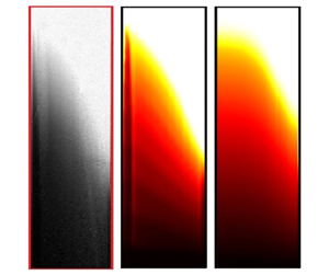
According to the exposure time, which is set to capture the images with appropriate lightness, the frame rate is calculated as two frames per second. The frame-to-frame evolution of pixel intensity gives a qualitative visualization of the flow. In grey scale, the intensity ranges from 0 (black) to 255 (white). To process the images, we first increase the contrast of all the original frames to improve the image quality. Then we normalize the intensity values using the reference difference  $(I_{init}-I_{final})$ which represents the intensity range of the annulus: either with only the transparent displaced fluids or with only the black displacing fluid, separately. The normalized intensity value is then
  $I_{nor} = (I_{init}-I)/(I_{init}-I_{final})$, so that 1 represents pure black (displacing fluid) and 0 represents pure white (displaced fluid). Using this normalization gives a suitable scale for the intensity signal of interest which is then later interpreted as a concentration field, i.e.
  $I_{nor} \in [0,1]$.
2.2. Computational models
The miscible displacement flow experiments in our apparatus are modelled using two complementary techniques. First, a 3-D computation is conducted using a volume of fluid (VOF) method, which in principle should be able to represent the observed experimental features, including dispersion and mixing. Second, a D2DGA model is used that is a form of the narrow-gap Hele-Shaw model, modified to allow for dispersive flows on the scale of the annular gap. These are outlined below.
2.2.1. The 3-D model
The 3-D model used is a finite volume method within the open source computational fluid dynamics toolbox OpenFOAM (http://www.openfoam.com). The geometry is built based on the experimental set-up, with local grid refinement close to the walls. A total of  $20 \times 100 \times 800$ cells are given in the radial, azimuthal and axial directions, respectively. Mesh sensitivity/convergence results are given by Sarmadi et al. (Reference Sarmadi, Renteria and Frigaard2021). The solver used is based on the twoLiquidMixingFoam case in the OpenFOAM library. This code has been successfully used for modelling miscible displacement flows in a pipe (Etrati & Frigaard Reference Etrati and Frigaard2018), in eccentric annuli with horizontal orientation (Sarmadi et al. Reference Sarmadi, Renteria and Frigaard2021) and in Part 1 of this study (Zhang & Frigaard Reference Zhang and Frigaard2022).
The annulus is initially full of displaced fluid. After the initial time, the displacing fluid is injected at the inlet, where a uniform velocity is imposed. The full Navier–Stokes equations are solved, coupled to an advection equation for the concentration of displacing fluid. The VOF method is used to capture the displacement front between the fluids. The momentum, continuity and concentration equations are
 \begin{gather} \hat{\rho}\left(\frac{\partial \hat{\boldsymbol{u}}}{\partial \hat{t}}+\hat{\boldsymbol{u}}\boldsymbol{\cdot} \hat{\boldsymbol{\nabla}} \hat{\boldsymbol{u}} \right)={-}\hat{\boldsymbol{\nabla}} \hat{p}+\hat{\boldsymbol{\nabla}}\boldsymbol{\cdot}\hat{\boldsymbol{\tau}} +\hat{\rho}\hat{\boldsymbol{g}}, \end{gather}
 \begin{gather}\hat{\boldsymbol{\nabla}}\boldsymbol{\cdot}\hat{\boldsymbol{u}}=0, \end{gather}
 \begin{gather}\frac{\partial c}{\partial \hat{t}}+\hat{\boldsymbol{u}} \boldsymbol{\cdot} \hat{\boldsymbol{\nabla}} c=0. \end{gather}
Here,  $\hat {\boldsymbol {u}}$ and
  $\hat {p}$ are the velocity and pressure;
  $\hat {\boldsymbol {\tau }}=\hat {\mu }\hat {\dot {\boldsymbol {\gamma }}}(\hat {\boldsymbol {u}})$ is the deviatoric stress tensor, with
  $\hat {\dot {\boldsymbol {\gamma }}}$ the rate of strain tensor. Dimensional quantities are denoted with the ‘hat’ accent, e.g.
  $\hat {p}$. No-slip conditions are applied at the annulus walls and outflow conditions at the outlet. The pressure is fixed at the outlet. The PIMPLE algorithm is used to solve the momentum equation and an implicit second-order Crank–Nicolson method is employed for the time discretization. All computations are carried out in parallel on a multi-processor machine, generally using 48 cores.
In this paper, we only consider two Newtonian fluids. It is possible to include a diffusion term in the right-hand side of (2.3), but the Péclet number ( $Pe$) calculated for the cases in our study is typically large enough that diffusion may be neglected (typically
  $Pe \geqslant 10^{5}$). To resolve diffusive effects with
  $Pe$ in this range requires very fine meshes. In practice, the VOF method results in intermediate concentrations, but over a limited front thickness. These intermediate concentrations are advected (dispersed) by secondary flows, so that many flows end up with significant mixed regions, as in the experiments. The concentration
  $c \in [0,1]$ enters the momentum equation only via the fluid properties:
  $\hat {\rho }$ and
  $\hat {\mu }$ are the mixture density and viscosity, defined by
 \begin{gather} \hat{\rho} =(1-c)\hat{\rho}_{1}+c\hat{\rho}_{2}, \end{gather}
 \begin{gather}\hat{\mu}=\hat{\mu} _{1}\exp \left[c\log \left(\frac{\hat{\mu} _{2}}{\hat{\mu}_{1}}\right)\right]. \end{gather}
Gradients in  $\hat {\rho }(c)$ contribute to significant buoyancy effects on these flows.
2.2.2. The dispersive 2-D gap-averaged model (D2DGA)
The D2DGA model was developed by Zhang & Frigaard (Reference Zhang and Frigaard2022) to be able to better account for dispersive effects on the scale of the annular gap, while preserving the computational advantages of a 2-D model, which is needed to simulate the flows that occur on the scale of a typical well. The key assumption is that the mean annular gap is much narrower compared to both the mean circumference and to the length-scale of any axial geometric variations. The narrow gap approximation requires that  $\delta /{\rm \pi} \ll 1$, as in our experimental set-up. Additionally, the Hele-Shaw approach requires
  $Re \delta /{\rm \pi} \ll 1$ for the inertial effects to be neglected. Based on these assumptions, the 3-D flow is reduced to a 2-D approximation by averaging the velocity and fluid concentration profiles in the radial direction. The radially averaged concentration of the displacing fluid will be denoted by
  $\bar {c}_r$, with the subscript denoting the direction of the average.
Gap-averaged 2-D approaches were developed by Bittleston et al. (Reference Bittleston, Ferguson and Frigaard2002) and Maleki & Frigaard (Reference Maleki and Frigaard2017), covering laminar, transitional and turbulent flows. The D2DGA model has similar derivation, but with different assumptions made regarding the distribution of fluids across the annular gap. It is assumed that the displacing fluid (fluid 2) can disperse (symmetrically) up through the centre of the local annular gap, whereas other 2-D approaches assume the fluid concentrations are uniform across the gap. For turbulent flows (Maleki & Frigaard Reference Maleki and Frigaard2017), this is reasonable, but for laminar flows, gap-scale dispersion is readily observed in experiments and 3-D computations.
The D2DGA model is given below in (2.6)–(2.8), written in dimensionless form, for two Newtonian fluids in laminar flow:
 \begin{gather} \frac{\partial}{\partial t}[Hr_{a}\bar{c}_r]+ \boldsymbol{\nabla}_a \boldsymbol{\cdot} \boldsymbol{q} = 0, \end{gather}
 \begin{gather}\boldsymbol{\nabla}_{a} \boldsymbol{\cdot} ( 2r_a H\bar{v},2r_a H\bar{w}) = 0, \quad \Rightarrow \frac{\partial \varPsi }{\partial \phi }=2Hr_{a}\bar{w}, \quad \frac{\partial \varPsi }{\partial \xi }={-}2H\bar{v}, \end{gather}
 \begin{gather}\boldsymbol{\nabla}_a \boldsymbol{\cdot} [\boldsymbol{S} + \boldsymbol{b}] = 0. \end{gather}
Equation (2.6) is a transport equation for the fluid 2 gap-averaged concentration  $\bar {c}_r$. The scaled annular half-gap-width is
  $H(\phi,\xi )$ and the mean radius at depth
  $\xi$ is
  $r_a(\xi )$ (
 $=1$ in a uniform annulus). Again, the effects of molecular diffusion are minimal on the time scales and length scales of relevance. Thus, diffusive effects are absent on the right-hand side of (2.6). The areal flux of fluid 2,
  $\boldsymbol {q}$, is given by
 \begin{gather} \boldsymbol{q} = (q_\phi , q_\xi ) =\! \frac{ r_a}{2} \left(- \frac{\partial \varPsi}{\partial \xi } , \frac{1}{r_a}\frac{\partial \varPsi}{\partial \phi } \right) \bar{c}_r \left[ \frac{m\bar{c}_r^2 + 1.5(1-\bar{c}_r^2)}{m\bar{c}_r^3 + 1\!-\!\bar{c}_r^3}\right] + \frac{{\rm \Delta} \rho H^3}{6 \eta_2} \mathcal{I}_3(\bar{c}_r,m)[{-}f_\xi,f_\phi ], \end{gather}
 \begin{gather}\mathcal{I}_3 = \frac{\bar{c}_r^2(1-\bar{c}_r)^3[4m\bar{c}_r + 3(1-\bar{c}_r)]}{2m[m\bar{c}_r^3 + 1 - \bar{c}_r^3 ]}, \end{gather}
where  $\eta _1$ and
  $\eta _2$ are the scaled viscosities, and
  ${\rm \Delta} \rho$ the density difference. Bittleston et al. (Reference Bittleston, Ferguson and Frigaard2002) define the flux terms as simply the multiple of the averaged concentration and averaged velocity:
  $\boldsymbol {q} = (\bar {v}\bar {c}_r, \bar {w}\bar {c}_r)$. Here we observe there is also a buoyancy contribution.
The gap averaged velocity field is incompressible, allowing it to be expressed in terms of a stream function  $\varPsi$, i.e. (2.7a,b). The operator
  ${\nabla}_{a}$ is a radial divergence operator, i.e.
 \begin{equation} \nabla_{a} = \left( \frac{1}{r_{a}}\frac{\partial }{\partial \phi }, \frac{\partial }{\partial \xi } \right), \end{equation}
with  ${\nabla} _{a}$ the corresponding gradient operator. The stream function satisfies the elliptic equation (2.8), with
 \begin{equation} \boldsymbol{S} =
\frac{3r_a }{2H^3} \frac{{\nabla}_a
\varPsi}{\displaystyle{\frac{\bar{c}_r^3}{\eta_2}
+\frac{(1-\bar{c}_r^3)}{\eta_1}}}, \quad \Rightarrow \tau_w
= \frac{3}{2H^2} \frac{|{\nabla}_a
\varPsi|}{\displaystyle{\frac{\bar{c}_r^3}{\eta_2} +
\frac{(1-\bar{c}_r^3)}{\eta_1}}}.
\end{equation}
\begin{equation} \boldsymbol{S} =
\frac{3r_a }{2H^3} \frac{{\nabla}_a
\varPsi}{\displaystyle{\frac{\bar{c}_r^3}{\eta_2}
+\frac{(1-\bar{c}_r^3)}{\eta_1}}}, \quad \Rightarrow \tau_w
= \frac{3}{2H^2} \frac{|{\nabla}_a
\varPsi|}{\displaystyle{\frac{\bar{c}_r^3}{\eta_2} +
\frac{(1-\bar{c}_r^3)}{\eta_1}}}.
\end{equation}
The function  $\boldsymbol {S}$ represents the dimensionless modified pressure gradient in the flow, and
  $\tau _w$ is the wall shear stress. An interpretation of (2.12) is that it represents an interpolation of the viscosity values of the two fluids, for which dispersion effects would be correctly represented. Bittleston et al. (Reference Bittleston, Ferguson and Frigaard2002) simply linearly interpolated the rheological parameters.
There are two parts to the buoyancy field:
 \begin{equation} \boldsymbol{b} = \left( \rho - \frac{{\rm \Delta} \rho}{H}\frac{\mathcal{I}_2}{\mathcal{I}_1} \right) \boldsymbol{f}. \end{equation}
The first part represents changes in the mean density in the direction  $\boldsymbol {f}$. These buoyancy gradients are exactly those considered in the models of Bittleston et al. (Reference Bittleston, Ferguson and Frigaard2002) and Maleki & Frigaard (Reference Maleki and Frigaard2017). The second part is obtained specifically from the layered flow. In other words, the effect of the layered flow on buoyancy is significant. The functions
  $\mathcal {I}_1$ and
  $\mathcal {I}_2$ are given by
 \begin{equation} \mathcal{I}_1 = H^3\left(\frac{\bar{c}_r^3}{3 \eta_2 } + \frac{1- \bar{c}_r^3}{3 \eta_1 } \right),\quad \mathcal{I}_2 = H^4\left[ \frac{(1-\bar{c}_r)\bar{c}_r^3}{3 \eta_2 } + \frac{\bar{c}_r(1-\bar{c}_r)^2(1+2 \bar{c}_r)}{6 \eta_1} \right] . \end{equation}
In more detail, the buoyancy term can be written as
 \begin{gather} \boldsymbol{\nabla}_a \boldsymbol{\cdot} \boldsymbol{b} = \boldsymbol{\nabla}_a \boldsymbol{\cdot} \left[ \rho_2 + {\rm \Delta} \rho \left( (1-\bar{c}_r) - \left[ \frac{m\bar{c}_r^3(1-\bar{c}_r) + \bar{c}_r(1-\bar{c}_r)^2(0.5+\bar{c}_r)}{m\bar{c}_r^3 + 1 - \bar{c}_r^3} \right] \right) \right] \boldsymbol{f}, \end{gather}
 \begin{gather}\boldsymbol{f} = \left( \frac{r_a \cos \beta }{{F^2}},\frac{r_a \sin \beta \sin {\rm \pi}\phi}{{F^2}}\right), \end{gather}
where  $F$ is the Froude number.
As the underlying mathematical structure of the 2DGA and D2DGA models is the same, the computational procedure is similar, with some additional cost from evaluating the new closure functions. The equations are discretized on a regular rectangular mesh, with a staggered mesh for the stream function versus concentration. At each time step, we first compute the rheological parameters as a function of concentration. Then we solve the elliptic equation (2.8) for stream functions, which is linear for Newtonian fluids. Once the stream function is found, the new velocity field is obtained and fed to a solver for hyperbolic equation (2.6). The flux corrected transport scheme (FCT) is selected, due to its ability to capture shocks and handle other nonlinearities. Using the FCT method, a new value of  $\bar {c}_r$ is computed.
2.3. Example results
Later we present results from the experiments, compared with both 3-D and D2-DGA models. Here we establish the basis of this comparison. Figure 2 is an illustration of a normalized experimental image, i.e. constructed from the intensity  $I_{nor}$. We have scaled the annulus length-to-width ratio in the image to allow viewing of a single section of the annulus. This figure depicts a displacement in the last section of the annulus, with figure 2(a–d) indicating the wide side view, the frontal view, the narrow side view and the back view, respectively. The two hazy blocks in the narrow side view represent mechanical supports of the annulus. For this case, the eccentricity is 0.8, the buoyancy number is 150 and the viscosity ratio is 0.8.

Figure 2. Example of an experimental result from the last section with (a) the wide side view; (b) the frontal view; (c) the narrow side view; (d) the back view. The dimensionless parameters are  $(e, b, m, Re) = (0.8, 150, 0.8, {29})$.
The wide side view reveals a rather uniform distribution of displacing fluid (dark colour), suggesting an efficient displacement. However, on moving from wide side to narrow side, we see that there are parts of the annulus that are not displaced. Particularly evident is a residual fluid channel along the narrow side, i.e. the vertical white strip in the centre of figure 2(c). Generally, the frontal view is clearer compared to the other views, which are reflected by the mirror system. In both the frontal view and the back view, we can see a long dark spike on the wide side, which is a finger of displacing fluid advancing along the centre of the annular gap. The discernible axial dispersion ahead of the dark front in the wide side view corresponds to viewing through this spike profile, which extends azimuthally in the centre of the annular gap, but is not present on the narrow side.
It is natural to interpret  $I_{nor}$ as a concentration of the displaced fluid, although this overlooks nonlinear dependence of the light absorption on the concentration. Considering the frontal image, for example, we may set
  $\tilde {C}_x(\hat {y},\hat {z},\hat {t}) = I_{nor}$ for each image, with
  $(\hat {y},\hat {z})$ directions across the image and along the vertical flow direction, respectively. Note that each
  $I_{nor}$ value has effectively averaged the light intensity in the third (depth) direction
  $x$, as indicated by the subscript
  $\bar {C}_x$. As discussed by Renteria & Frigaard (Reference Renteria and Frigaard2020), the annulus is difficult to control reflections and lighting effects, so that direct interpretation of
  $\tilde {C}_x(\hat {y},\hat {z},\hat {t})$ in this way is always uncertain.
Despite the above uncertainty, we still wish to compare with 3-D computations of the colour function  $c$. To do this, we post-process the 3-D results. Figure 3(a) shows schematically an axonometric graph of an eccentric annulus displacement. We now take the 3-D concentration
  $c(\hat {x},\hat {y},\hat {z},\hat {t})$ and average in the
  $\hat {x}$-direction, as illustrated in figure 3(b). This depth average, denoted
  $\bar {c}_{x}(\hat {y},\hat {z},\hat {t})$, is now compared qualitatively with the frontal view obtained from the cameras. We will also compare with the gap-averaged
  $\bar {c}_r$ computed from the D2DGA model. Comparing radially averaged and depth-averaged profiles is at best qualitative. Zhang & Frigaard (Reference Zhang and Frigaard2022) radially averaged the 3-D model results to compare with the 2DGA and D2DGA models.

Figure 3. Schematic of (a) an axonometric graph of an eccentric annulus (the blue edges represent the meshes generated in 3-D simulations) and (b) how we average the concentration values in the depth direction for each axial slice, regarding the images taken from the frontal view.
3. Results
Central to primary cementing is the notion of a steady-state displacement, in which the displacement front advances at the mean pumping speed. Self-evidently, the steady-state displacement represents perfect mud removal and cement placement. Some 30 years ago, the idea was captured in rule based design systems such as that of Couturier et al. (Reference Couturier, Guillot, Hendriks and Callet1990), which used hydraulic analogies to infer when there would be a zero differential velocity between interface speeds on the wide and narrow sides of the annulus. The earliest 2-D gap-averaged models showed that steady-state displacements were theoretically feasible (Pelipenko & Frigaard Reference Pelipenko and Frigaard2004a) and computed them (Bittleston et al. Reference Bittleston, Ferguson and Frigaard2002; Pelipenko & Frigaard Reference Pelipenko and Frigaard2004b). Methods to predict their occurrence were also derived (Frigaard & Pelipenko Reference Frigaard and Pelipenko2003; Pelipenko & Frigaard Reference Pelipenko and Frigaard2004c). However, even though steady-state displacements exist mathematically in the 2DGA model of Bittleston et al. (Reference Bittleston, Ferguson and Frigaard2002), once we explore the displacement flow in experiments or in 3-D simulations, it is immediately apparent that these miscible displacements are strongly affected by dispersion.
From where does this dispersion originate? In turbulent flow regimes, the fluids mix rapidly across the annular gap, leading to spreading of the displacement front via Taylor dispersion; see Maleki & Frigaard (Reference Maleki and Frigaard2017). However, laminar displacements are at high Péclet number, outside of the laminar Taylor dispersion regime. Thus, advective dispersion over shorter time scales must be accounted for in any realistic model: hence, the D2DGA model of Zhang & Frigaard (Reference Zhang and Frigaard2022). Laminar dispersion arises from at least two sources. First, there is dispersion due to the velocity and concentration profiles across the annular gap, which was the target of the D2DGA model. Second, there may be strong azimuthal flows. These are generally local to the displacement front and occur as fluid is driven from narrow to wide side ahead of the front, and vice versa behind the front. Lastly, there is dispersion associated with experimental operations and imperfections in the experimental apparatus, e.g. opening of the gate valve at the start of the experiment shears and mixes the fluids locally.
Although all displacements have a degree of dispersion, which acts to smear the displacement front, this does not invalidate the conceptual utility of a stable steady-state displacement in describing an effective flow from the industrial perspective. Thus, both experimentally and computationally, one must use some kind of threshold to determine whether the underlying displacement front may be deemed steady. For the experiments, there is the additional complication that observation is visual from a side view of the annulus. Thus, we cannot directly observe the gap-scale dynamics all around the annulus, as we can in 3-D computation, although some features are evident; see figure 2 and discussion.
Equally important is to recognise that both displacement front motion and dispersive smearing of the front by secondary flows are predominantly advective phenomena. Turbulent Taylor dispersion, laminar mixing and even laminar displacements in a horizontal annulus all lead to diffusive behaviour along the annulus. By focusing on vertically oriented annuli and on laminar flows, we hope to isolate and understand the advective aspects of these flows.
3.1. Displacements in concentric annulus ( $e=0$)

Azimuthal secondary flows are eliminated in principle by considering displacements in concentric annuli. Thus, here we first analyse our experiments with  $e=0$. This allows us to consider displacements affected primarily by gap-scale dispersion (and initial disturbances). In this way, we can develop sensible methods for the classification of different behaviours. We focus mainly on analysing the frontal view and considering other views when more detailed information is needed. Our first aim is to classify the displacements as either steady front or unsteady flows, by assessing the normalized front velocities from both experimental and computational aspects (§ 3.1.1). Then, we quantify the dispersion by computing the standard deviations of relative velocities of the front, compared with the imposed velocity (§ 3.1.2). Lastly, we summarize the effects of different dimensionless parameters in § 3.1.3 by classifying steady front or unsteady and dispersive/non-dispersive flows.
3.1.1. Classifying steady and unsteady advective behaviour via a similarity transform
The first task is meaningful to classify displacements as either a steady front or unsteady. Although ideally this should mean that the front advances at the mean pumping speed all around the annulus, dispersion will lead to a faster arrival of the displacing fluid. Equally, we have three methods for assessing the flow: (i) an imperfect experiment; (ii) 3-D simulation; and (iii) D2DGA simulations. Our approach is as follows. For the experiments, we begin by selecting images taken from the frontal view of the first and last sections at different time steps. We average the image  $\bar {C}_x(\hat {y},\hat {z},\hat {t})$ with respect to
  $\hat {y}$ to give
  $\bar {C}(\hat {z},\hat {t})$. Since we already averaged across the annular cross-section in the
  $x$-direction, the quantity
  $\bar {C}(\hat {z},\hat {t})$ represents the (experimental) mean concentration of displacing fluid at each distance, obtained by a cross-sectional area average. For the 3-D results, we have already averaged first in
  $\hat {x}$ to give
  $\bar {c}_x$, (comparable to the experimental image), and now also average with respect to
  $\hat {y}$ to give the cross-sectional area average
  $\bar {c}(\hat {z},\hat {t})$. Lastly, we average the D2DGA results with respect to the azimuthal direction. We also denote the latter as
  $\bar {c}(\hat {z},\hat {t})$. Since the radial coordinate was already averaged to predict
  $\bar {c}_r$, it follows that
  $\bar {c}(\hat {z},\hat {t})$ is also a cross-sectional area average.
Terms such as ‘front’ and ‘interface’ are always difficult when dealing with miscible displacements, as formally there is no interface. Equally, when we have significant dispersion, even for high-Péclet-number flows, the location of a nominal interface can become progressively smeared. Our visualization presents an image that is itself a type of average, hence vulnerable to dispersive smearing. A legitimate question is whether we can define a displacement front meaningfully at all that is applicable to the range of observed behaviours. To address this, we have focused on extracting the advective character of the flows. By plotting  $\bar {C}(\hat {z},\hat {t})$ or
  $\bar {c}(\hat {z},\hat {t})$ against the variable
  $\hat {z}/\hat {t}$ for successive images (time steps), we are able to discern if the displacement is primarily advective. In the case where the flow is advection dominated, the mean concentrations will collapse onto a master curve in
  $\hat {z}/\hat {t}$. Denoting the normalized similarity variable by
  $w_f=(\hat {z}/\hat {t})/\hat {w}_{0}$, we find the master curve for
  $\bar {C}(w_f)$ or
  $\bar {c}(w_f)$ (3-D and D2DGA). The values of
  $w_f$, plotted as a function of cross-sectionally averaged concentration, show the range of front velocities found via each method.
This method is equally applicable to a nice clean interface or a very diffuse one, as we will see below. When the similarity variable is defined for all  $\bar {C}$ (or
  $\bar {c}$), then the displacement front can be considered as the union of all the wavespeeds
  $w_f$. If the actual images were visualized, this visual representation might appear to be steady or otherwise, relatively clean or smeared. The ability to handle these different behaviours is the main attraction of using this method. The disadvantage is some ambiguity in defining the displacement front via
  $w_f$, as for cases of large dispersion, the actual image may not appear front-like at all.
Typically, the collapse of the averaged concentration onto the similarity variable  $\hat {z}/\hat {t}$ is imperfect at both small and large mean concentrations, requiring filtering. As a threshold for the experimental data, we adopt the same criterion as Renteria & Frigaard (Reference Renteria and Frigaard2020), that is, we categorize flows as having a steady front by
 \begin{equation} {\rm \Delta} w_f = w_f(\bar{C} =0.3)-w_f(\bar{C} =0.7) \le 0.1. \end{equation}
The flows are classified as unsteady otherwise. When steady, we refer to the steadily moving segment between  $\bar {C}=0.3$ and
  $\bar {C}=0.7$ as the main front. The front may of course extend beyond these threshold values, which are conservatively chosen. We start with a case of zero buoyancy force (EXP 5) for which
  $(e, b, m, Re) = (0, 0, 0.2, 50)$. Figure 4 shows a comparison of experiments, depth-averaged 3-D and D2DGA results. Figure 4(a–c) present the plotting of
  $\bar {C}$,
  $\bar {c}$ and
  $\bar {c}$ versus the similarity variable
  $w_f$, at a series of time steps, for the three methods. The experimental profiles are obtained only from the first and last sections, while the computational ones are computed from the entire annulus. For clarity, the mean concentrations when the front enters the last section of the annulus are plotted in green for the experiment, typically representing the most converged profiles, and the last profile computed is plotted for the simulations in green. Figure 4(d–f) display example displacement images from the first and last sections at two distinct time steps. The steps are chosen to be illustrative, and represent the same times for experiments and models. The same figure format is adopted subsequently.

Figure 4. Case EXP 5 with  $(e, b, m, Re) = (0, 0, 0.2, 50)$. Panels (a–c) plot
  $\bar {C}$,
  $\bar {c}$ and
  $\bar {c}$, from experiment, 3-D simulation and D2DGA models, respectively. The curves are collapsed onto the similarity variable
  $w_f=(\hat {z}/\hat {t})/\hat {w}_{0}$, representing the scaled front speed. The black and green curves in (a) represent the profiles of averaged concentration from the first and last section of the annulus from experimental results. The black profiles in (b,c) are computed from the entire annulus. Panels (d–f) show illustrative images (
 $\bar {C}_{x}$) from the frontal view of the experiment in (d), the depth averaged 3-D computation
  $\bar {c}_{x}$, in (e) and the D2DGA radially averaged concentrations
  $\bar {c}_r$ in (f). The times for experiment and simulations are the same. One image is taken from when the front is in the first section of the annulus and the other one from the fourth section of the annulus.
We observe that for the 3-D and D2DGA computational results, the data collapse very well onto a master curve  $\bar {c}(w_f)$. However, the experimental data do not collapse well for this particular experiment (figure 4a), instead showing pronounced fluctuations. Additionally, the experimental curves appear to show larger maximum front velocity, whereas the models both have a peak front speed of approximately 1.5. The latter is consistent with dispersion along a plane channel. It is apparent that for this iso-dense case,
  ${\rm \Delta} w_f = w_f(\bar {C}=0.3)-w_f(\bar {C}=0.7)> 0.1$ from experimental and computational results, which indicates a typical unsteady flow.
Why the experimental results do not collapse onto a master curve  $\bar {C}(w_f)$ and why we see peak front velocities significantly larger is probably due to a combination of factors. Reflections have a significant impact on the pixel values recorded. Therefore, the experimental results are not as distinct as the computational results in any of our experiments. There are also likely to be minor non-uniformities in the apparatus, deviating from truly concentric. Although the displacing fluid is more viscous (
 $m = 0.2$), this is the only stabilizing feature of the flow that might lead to a uniform and efficient displacement.
Looking at figure 4(d,e), we observe darker profiles close to the edges of the image, which are effectively the displacement front viewed in the annular gap on each side. This is consistent with a Poiseuille-type flow on the gap scale: with a dispersive spike that advances along the centre of the annular gap, leaving behind residual layers on both walls. The depth-averaged 3-D results capture this behaviour as well as the experiments. In the D2DGA model, this effect is implicitly included in the model. Whereas the thin spike produces near identical behaviour in the two models, in the experiment, we see that the spike is intermittent on the two sides and the images are also not uniform in  $\hat {y}$, with some channelling occurring in the last section; see the clear white zone at the top left of the last section of figure 4(d). This asymmetry likely allows the (averaged) front to advance faster than in either model.
Now if we turn to look at a case (EXP 96) with large buoyancy number ( $b=750$), figure 5 shows a quite different result. First, we can observe a flat front and complete displacement from the first to last sections through all of the results shown in figure 5(d–f). Second, the average concentration in the
  $\hat {y}$-direction collapses onto a master curve
  $\bar {c}(w_f)$, which clearly shows a steadily advancing front (with speed close to
  $w_f = 1$); see figure 5(a–c). This indicates an ideal steady front displacement with minimal dispersion. For the experimental results in figure 5(a), the series of curves from the first section has not converged as completely as those from the last section. For the model data, the last curve
  $\bar {c}(w_f)$ plotted has been coloured green, from which we can see the convergence. In all cases, the criterion (3.1) is satisfied. Compared with the previous example, it is evident that the buoyancy force is primarily responsible for limiting gap-scale dispersion, leading to the steady front displacement.

Figure 5. Case EXP 96 with  $(e, b, m, Re) = (0, 750, 0.2, {29})$. Panel (a–c) plot
  $\bar {C}$,
  $\bar {c}$ and
  $\bar {c}$ from experiment, 3-D simulation and D2DGA models, respectively. The curves are collapsed onto the similarity variable
  $w_f=(\hat {z}/\hat {t})/\hat {w}_{0}$, representing the scaled front speed. The black and green curves in (a) represent the profiles of averaged concentration from the first and last sections of the annulus from experimental results. The green curves in (b,c) show the result of the last time step which are computed from the entire annulus. Panels (d–f) show illustrative images (
 $\bar {C}_{x}$) from the frontal view of the experiment in (d), the depth averaged 3D computation
  $\bar {c}_{x}$ in (e) and the D2DGA radially averaged concentrations
  $\bar {c}_r$ in (f). The times for experiment and simulations are the same. One image is taken from when the front is in the first section of the annulus and the other one from the fourth section of the annulus.
There are two additional observations from figure 5. First, the dispersion ahead of the front in figure 5(d) grows more rapidly than in the computational results. This has been observed in others of our experiments, typically at lower flow rates. Some initial mixing occurs when the gate valve is opened, but before the mixed fluid enters the annulus, which could be the cause. A similar phenomenon has been observed and explained in the work of Etrati & Frigaard (Reference Etrati and Frigaard2018), which studied miscible displacement flows in an inclined pipe with density stable configuration. Alternatively, it may be related to approaching the lower flow rate limit of the pump, where fluctuations may grow. Note that apart from controlling density, large  $b$ in our experiments is controlled by setting a low flow rate.
The second observation is that in terms of predicting the changing front velocity and concentration distribution along the annulus, the D2DGA model produces more dispersion than the 3D model in this particular case. We see in figure 5(d) that the dispersive spikes are present in the annular gap and grow longer in § 4 of the annulus. However, compared with figure 4(d), they appear to extend less along the annulus and to be thinner. This feature should not be suppressed in the 3-D simulation and is still visible on close inspection. It could be that dispersive spikes are too small to be fully represented by the 3-D mesh. However, they influence the D2DGA approach directly as they are implicitly modelled. This may explain why the D2DGA model disperses more.
3.1.2. Dispersive or non-dispersive
Intuitively, an unsteady flow is always accompanied by a significant degree of dispersion; indeed unsteadiness is a form of dispersion. Many unsteady flows arise due to eccentricity (Pelipenko & Frigaard Reference Pelipenko and Frigaard2004c), but here we consider only  $e=0$, so is dispersion still inevitable and also for steady front flows? According to our visual observations, in experiments and 3-D simulations, there is dispersion on the scale of the annular gap, which leads to a smearing of 2-D images of the flows. However, we have seen very clear steady fronts as well, so the question is how to identify a threshold that can be used to define different regimes and degrees of dispersion. We first present a steady front flow (figure 6) with smaller buoyancy number (EXP 48) and compare it with the case introduced previously (figure 5) to explore these differences. Ideally, we would like to quantify the dispersive effects in a way that is distinct from unsteadiness.

Figure 6. Case EXP 48 with  $(e, b, m, Re) = (0, 30, 0.8, {144})$. Panels (a–c) plot
  $\bar {C}$,
  $\bar {c}$ and
  $\bar {c}$ from experiment, 3-D simulation and D2DGA models, respectively. The curves are collapsed onto the similarity variable
  $w_f=(\hat {z}/\hat {t})/\hat {w}_{0}$, representing the scaled front speed. The black and green curves in (a) represent the profiles of averaged concentration from the first and last section of the annulus from experimental results. The green curves in (b,c) show the results of the last time step which are computed from the entire annulus. Panels (d–f) show illustrative images (
 $\bar {C}_{x}$) from the frontal view of the experiment in (d), the depth averaged 3-D computation
  $\bar {c}_{x}$ in (e) and the D2DGA radially averaged concentrations
  $\bar {c}_r$ in (f). The times for experiment and simulations are the same. One image is taken from when the front is in the first section of the annulus and the other one from the fourth section of the annulus.
Similar to figure 5, we find that the convergence of the experimental profiles is incomplete in the first section of the annulus, but not the last. The green lines in the computational results (figure 6b,c) again represent the last time steps calculated. Although there are significant variations in  $w_f(\bar {c})$, both for low and high
  $\bar {c}$, the main front (at intermediate values of
  $\bar {c}$) evolves steadily and the criterion (3.1) is satisfied. However, we note that the main front has speed
  $w_f > 1$.
Second, compared with figure 5, we see significantly more dispersion. This is signalled in particular by the part of the converged  $w_f$ profile at low
  $\bar {C}$. Rather than referring to this again as a ‘spike’, to avoid confusion, we call this feature a leading front: meaning the part of the front that advances ahead of the main front, which we threshold at
  $\bar {C} < 0.15$ to distinguish from the lower limit of the main front. Figure 6(c) marks this feature with a blue dashed rectangle. It corresponds to the region with light grey or yellow colour in the illustrative images in figure 6(d–f). There are always larger values for the first displacing fluids, but in cases such as in figure 5, these features are barely noticeable, occurring in the range of measurement error of
  $\bar {C}$ for the experiments. The leading front in figure 6 is however more substantial and signifies fluid dispersion ahead of the main front, as seen clearly in comparison to figure 5 for all three methods of approximating. Also notable is that the leading front has significantly increased in the fourth section compared with the first. On close inspection of the concentration images, we can also see that the spikes in concentration at the local gap scale (marked with circles) are significantly longer here than in figure 5.
At large  $\bar {c}$, the front speed lags behind the main front speed quite significantly in the computed profiles, but less so in the experiment. This part of the curve represents the slower displacement of the wall layers around the annulus. This is calculated effectively in 3-D and is implicitly part of the fluxes in the D2DGA model. However evidently, visualizing the experiment from a side view is less effective at capturing these particular flow features. This is not surprising as in the experimental annulus, we have no means of ‘back-lighting’ the inner pipe to allow a more objective quantification of light absorption in the fluid layers between pipe and outer wall.
To have a better understanding of what is happening within the annular gap, we explore a slice along the annular gap, at fixed  $\hat {x}=0$, using the 3-D results for both EXP 48 and EXP 96; figure 7. In the colour maps,
  $c=1$ represents the pure displacing fluid and the vectors show the normalized velocity. A long thin dispersive spike and obvious residual layers close to the walls can be observed in figure 7(a). It is the side view of such features that we see in the experimental images at the two sides of the annulus. The displacement in figure 7(b) is much more piston-like. Note that the axial velocity has a Poiseuille-type distribution that is observable both upstream and downstream in figure 7(a), away from the front. In the second case however, a more uniform velocity distribution can be observed in every axial position (figure 7b), which is due to secondary flows driven by the strong buoyancy force.

Figure 7. Displacement flow near the front for (a) case EXP 48  $(e, b, m, Re) = (0, 30, 0.8, {144})$; (b) case EXP 96
  $(e, b, m, Re) = (0, 750, 0.2, {29})$. The colour map presents concentrations across the channel gap where
  $\hat {x}=0$ (
 $c=1$ represents pure displacing fluid). The vector field shows the axial velocity.
Conservation properties of the 3-D code are generally good; see Sarmadi et al. (Reference Sarmadi, Renteria and Frigaard2021). Numerical diffusion is limited generally to 1–2 cells, e.g. see the thickness of the diffuse layer in figure 7(a), close to the wall, which is fairly characteristic. However, these thin diffuse layers are effectively dispersed in parts of the flow where the velocity difference is significant, as seen further downstream in figures 7(a) or 7(b). This is not an effect of neglecting molecular diffusion (high-Péclet-number approximation). The numerical effects would dominate physical diffusion. Taking values for water and the typical pumping speeds in the apparatus, the diffusive length scale at the exit of the annulus is  $\sim$1 mm at most. As observed, the dispersive effects in the streamwise direction are significantly larger than this. However, it is possible that there could be a physical effect on the wall layer removal process. A finer mesh would better represent the spike in figure 7(a).
We have observed quite different gap-scale velocity fields associated with the different dispersion patterns. Although worthy of deeper study, the aim here is mainly to quantify different dispersion effects. We have seen in figure 6 that the pattern of dispersion ahead and behind the main front, when the displacement is steady front, has a different character. This is captured in the converged profiles  $\bar {c}(w_f)$, which may equally be plotted as
  $w_f(\bar {c})$. On subtracting the mean pumping speed, we may define the (dimensionless) relative velocity:
  $w_r(\bar {c}) = w_f(\bar {c}) - 1$. We divide the relative velocity field into two components:
  $w_{r}^{+}$ and
  $w_{r}^{-}$, corresponding to the positive and negative parts of
  $w_{r}$, respectively. The values of
  $\bar {c}$ associated with
  $w_{r}^{+}$ characterize the dispersion downstream, moving faster than the mean flow front. Those
  $\bar {c}$ associated with
  $w_{r}^{-}$ characterize the dispersion upstream of the mean flow front, e.g. with slow removal of residual wall layers. We quantify the degree of dispersion by calculating the standard deviation at late times for each case:
 \begin{gather} \sigma_{w_{r}^{+}}=\sqrt{\frac{1}{n_{+}}\sum_{0<\bar{c}<1} (w^{+}_{r}(\bar{c}))^{2}}, \end{gather}
 \begin{gather}\sigma_{w_{r}^{-}}=\sqrt{\frac{1}{n_{-}}\sum_{0<\bar{c}<1} (w^{-}_{r}(\bar{c}))^{2}}. \end{gather}
Here,  $n_+$ and
  $n_-$ indicate the total number of points involved in the summation calculations. Although the above calculation could be expressed as integrals, in practice, we treat the computed results in the same way as the experimental, segmenting
  $\bar {c}$ and summing over a finite number of discrete
  $\bar {c}$ values.
The results obtained are listed in table 3. As observed earlier, the side view in the experiments does not allow proper quantification of the upstream residual wall layers. Thus, only  $\sigma _{w_{r}^{+}}$ is computed for the experiments, and uses data from the fourth section of the annulus (
 $3.6m\le \hat {z}\le 4.8m$), late in the experiment. The 3-D and D2DGA results are cleaner and clearer, so we use the entire annulus for evaluating
  $\sigma _{w_{r}^{+}}$ and
  $\sigma _{w_{r}^{-}}$. According to table 3, the dispersion along the whole annulus in EXP 48 is greater than that in EXP 96, as quantified by all methods. There are discrepancies between
  $\sigma _{w_{r}^{+}}$ calculated from the different models and experiment, with the experimental values the largest. However, the order of magnitude is similar and exposes differences between the two experiments. Similarly for comparisons between
  $\sigma _{w_{r}^{-}}$. We have also tested many other cases, not shown here for reasons of brevity. As a result, we conclude that
  $\sigma _{w_{r}^{+}} \le 0.08$ can be used as a threshold value to identify a non-dispersive steady front flow.
Table 3. Standard deviation  $\sigma _{w_{r}^{+}}$ calculated from experimental and computational results, and
  $\sigma _{w_{r}^{-}}$ calculated from 3-D and D2DGA results at a later time step, for case EXP 48 with
  $(e, b, m, Re) = (0, 30, 0.8, {144})$ and case EXP 96 with
  $(e, b, m, Re) = (0, 750, 0.2, {29})$.

However, even when  $\sigma _{w_{r}^{+}} > 0.08$, the picture is not so clear. In cases such as EXP 48, the main front speed is
  $w_f > 1$. Thus, the computation of
  $\sigma _{w_{r}^{+}}$ includes the average velocity difference between the front and the mean flow, plus any effects of the dispersive spike (from values at low
  $\bar {c}_{y}$). Interpretation of
  $\sigma _{w_{r}^{-}}$ is less ambiguous, in relating only to displacement of the wall layers. To distinguish between a main front speed (
 $w_f > 1$) and the dispersive effect of the spike, we calculate the areas of the regions enclosed by
  $w_{r}^{+}(\bar {c})$ and
  $w_{r}^{-}(\bar {c})$, again evaluated at late times in the displacement. We define two parameters
  $|\bar {w}_{r}^{+}|$ and
  $|\bar {w}_{r}^{-}|$ as follows:
 \begin{gather} |\bar{w}_{r}^{+}| =\int_{0}^{1} w_{r}^{+} \,{\rm d} \bar{c}, \end{gather}
 \begin{gather}|\bar{w}_{r}^{-}| ={-} \int_{0}^{1} w_{r}^{-} \,{\rm d} \bar{c}. \end{gather}
These give an indication of the total dispersive area ahead of the mean position of the front, and the residual fluid left behind, respectively. We can compute these with either model, but have not found distinct differences between D2DGA and 3-D results. Whereas the standard deviations are influenced by large deviations, the above measures are not. This allows us to differentiate between effects of a steady main front ( $w_f \gtrsim 1$) and dispersive spikes in the profile of
  $w_f$, as discussed with respect to figure 6.
To illustrate, we show a case (EXP 71) at intermediate  $b=150$; see figure 8. The concentration colourmaps suggest that this case is non-dispersive. However, the spike-type profile of
  $w_f$ at low concentrations results in a significant
  $\sigma _{w_{r}^{+}}$, resulting from peak values of
  $w_{r}^{+}$ close to 0.13, when
  $|\bar {w}_{r}^{+}|$ is quite modest. In table 4, the values calculated from the D2DGA results are listed and compared with EXP 48. A first observation is that the values of
  $|\bar {w}_{r}^{+}|$ and
  $|\bar {w}_{r}^{-}|$ are similar. Second, we see that although
  $\sigma _{w_{r}^{+}}$ is comparable between these cases,
  $|\bar {w}_{r}^{+}|$ is much smaller in EXP 71. Unlike EXP 48, the main front in EXP 71 is moving at a speed much closer to the mean speed, which means that
  $|\bar {w}_{r}^{+}|$ is reduced (with the main contribution coming from the dispersive spike)

Figure 8. The (a) 3-D and (b) D2DGA results of relative velocity  ${w}_r=((\hat {z}/\hat {t})-\hat {w}_{0})/\hat {w}_{0}$ of case EXP 71 with
  $(e, b, m, Re) = (0, 150, 0.2, {145})$; (c) 3-D depth-averaged and (d) D2DGA concentration colourmap in the first and last sections of the annulus. Green lines represent the trend computed from a later time step (
 $\hat {t}=0.8*\hat {z}(4.8m)/\hat {w}_{0}$).
Table 4. Areas  $|\bar {w}_{r}^{+}|$ and
  $|\bar {w}_{r}^{-}|$ calculated from D2DGA results at a later time step for case EXP 48 with
  $(e, b, m, Re) = (0, 30, 0.8, {144})$ and case EXP 71 with
  $(e, b, m, Re) = (0, 150, 0.2, {145})$.

On exploring different cases, we have determined that  $|\bar {w}_{r}^{+}|= 0.05$ is a reasonable threshold value for evaluating dispersion. To summarize, a dispersive flow is classified as such if both the following conditions are met:
 \begin{equation} \sigma _{w_{r}^{+}} > 0.08 \quad \mbox{and}\quad |\bar{w}_{r}^{+}| > 0.05. \end{equation}
The flow is classified as non-dispersive otherwise. Essentially, the above quantifies the degree of smearing of the front and that it is not solely coming from the dispersive spike that is observed on the gap scale.
3.1.3. Effects of dimensionless parameters
In summary, we have now established threshold criteria to determine whether a flow is steady front, unsteady, dispersive or non-dispersive. In this section, we will classify our cases with  $e=0$ and analyse further the effects of various dimensionless parameters. We also mention that some of our experimental data sets, particularly those with extremely high or low buoyancy numbers, can be classified visually. We only need to further analyse cases with moderate buoyancy force or if it is difficult to tell merely from the images. Having said this, as seen above, the values of the standard deviations and of
  $|\bar {w}_{r}^{\pm }|$ are also of interest for quantitative interpretation. We begin with the buoyancy number, which is often the dominant factor in primary cementing.
Keeping the viscosity ratio constant at  $m=0.2$, we select cases with varying buoyancy numbers. Note that the Reynolds number often also varies with the buoyancy number, as our main control of
  $b$ is via the flow rate. The classification is presented in figure 9. In general, we find good agreement for the classification results obtained from all methods, except for the case with zero buoyancy. From figure 9(a), it is evident that the flow becomes more steady as the buoyancy number
  $b$ increases, and a magnitude of
  $b \sim O(10)$ is sufficient to provide a steady front in concentric annulus. It is apparently detrimental to the displacement flow if the buoyancy force is too small between fluid pairs. In addition, the discrepancy between different methods is negligible when
  $b > 100$, indicating that both 3-D and D2DGA models could accurately predict the steady front pattern.

Figure 9. Classification for some of the designed cases with increasing buoyancy number, obtained from experimental and computational results as indicated by different symbols. The viscosity ratio is maintained constant at  $m=0.2$. (a) Steady front or unsteady flows determined by
  ${\rm \Delta} w_f$; (b) non-dispersive flows determined by
  $\sigma _{w_{r}^{+}}$; (c) dispersive or non-dispersive flows determined by
  $|\bar {w}_{r}^{+}|$.
With regards to the classification of dispersive and non-dispersive flows, it is notable from figure 9(b) that the relative front velocity can be 10 % greater than the mean flow velocity  $\hat {w}_0$, even when the buoyancy number is beyond 100. A piston-like displacement could be obtained only if the buoyancy number is increased to a very high level (
 $b \gtrapprox 10^3$). This confirms that the dispersive spike regime on the gap scale is common, but the quantity of dispersive fluids could be effectively limited if moderate buoyancy force is attained. As figure 9(c) shows, the flow is in the non-dispersive regime when
  $b> 100$, since the proportion of displacing fluids with faster velocity is small. Therefore, as a rough guideline for displacement flows in a concentric annulus, we transition to steady front flows with only minor dispersive effects for
  $b \gtrapprox 10^2$, with larger
  $b$ being beneficial. Both 3-D and D2DGA models are suitable at a design stage for accurate prediction. For most of our studies, the experimental results are more dispersive than the model results, but we have seen that part of this discrepancy is due to measurement error, i.e. the visualization system cannot detect all 3-D features across the gap.
The viscosity ratio  $m$ appears to have a secondary role in cementing displacement flows, as described by Renteria & Frigaard (Reference Renteria and Frigaard2020), Zhang & Frigaard (Reference Zhang and Frigaard2021, Reference Zhang and Frigaard2022), Zhang et al. (Reference Zhang, Jung, Renteria and Frigaard2022). Here, we have chosen two iso-dense cases with only differing viscosity ratios (
 $m = 0.2,2$), the Reynolds number is maintained at the same value and
  $e=0$. We only focus on computational results for a clearer analysis. We know from the previous papers that the viscosity ratio mainly affects the degree of dispersion, so we plot the spatio-temporal colour map from D2DGA results in figure 10(a,b) to provide a more intuitive understanding. The region between the two dashed lines represents the concentration range from 0.1 to 0.9. In addition, the normalized front velocity is presented in figure 10(c,d). We also provide 3-D results as comparisons in the insets.

Figure 10. The D2DGA results of (a) spatio-temporal plot of concentration of case EXP 5 with  $(e, b, m, Re) = (0, 0, 0.2, 50)$; (b) spatio-temporal plot of concentration of case EXP 8 with
  $(e, b, m, Re) = (0, 0, 2.0, 50)$; the region within two dashed lines represents the concentration range from 0.1 to 0.9; (c)
  $\bar {c}$ versus
  $w_f$ of case EXP 5; (d)
  $\bar {c}$ versus
  $w_f$ of case EXP 8. The 3-D results of
  $\bar {c}$ versus
  $w_f$ are shown in the inset for comparison.
Focusing on the area enclosed by the dashed lines, the first case ( $m=0.2$) shows a narrower region but more uniform variation of concentration. For the second case, although there is a clearer sharp front for low values of
  $\bar {c}_{\hat {y}}$, the wider region between the dashed lines indicates that a greater quantity of fluids are dispersing: both cases are unsteady and dispersive if we calculate
  ${\rm \Delta} w_f$ and
  $\sigma _{w_{r}^{+}}$. However, the area deviating from the mean pumping velocity is larger for the second case, with larger viscosity ratio. Specifically,
  $|\bar {w}_{r}^{+}|=0.1446$ in case EXP 5 (
 $m=0.2$) and
  $|\bar {w}_{r}^{+}|=0.2214$ in case EXP 8 (
 $m=0.8$). We find the same trend and similar values in our 3-D results. To summarize, the viscosity ratio affects the dispersive pattern to some extent and it is not beneficial to increase to
  $m>1$, as is intuitive. More dispersion along the whole annulus will result in a lower displacement efficiency if the pumping time is fixed. However, we confirm that viscosity ratio effects, as studied, are still secondary for large
  $b$. The viscosity ratio only needs to be carefully considered and designed if
  $b$ is fairly low (say
  $b <30$).
3.2. Displacements in eccentric annulus ($e>0$)

We now turn to examine more realistic scenarios in which the annulus is eccentric. A degree of offset between the casing and wellbore is always present in primary cementing, despite the deployment of centralizers to position the casing more centrally in the hole. Eccentricity is widely acknowledged as one of the dominant factors affecting the displacement, simply because the fluids move faster in the wider gap. Here we first explore the competition between buoyant force and eccentricity by presenting a series of cases, then we classify the flow regimes using the criteria introduced for concentric annuli.
3.2.1. $b=0$

We start from the cases with zero buoyancy force to intuitively realize the effect of eccentricity. Figure 11 shows a displacement process for three cases with varying eccentricities ( $e=0.2, 0.4, 0.8$, respectively), with otherwise identical parameters. As in § 3.1, figure 11(d–f) show comparative colourmaps between experimental frontal image, averaged 3-D and D2DGA results, at a single time. Figure 11(a–c) plot
  $\bar {c}_{\hat {y}}$ against the front velocity
  $w_f$, obtained from the computational results late in the displacement.

Figure 11. Graphs of  $\bar {c}$ versus
  $w_f$ obtained from computational results, and displacement process in the first section of the annulus presented by both experimental and computational (depth-averaged 3-D and D2DGA) results in the same time step, for the case (a,d) EXP 18 with
  $(e, b, m, Re) = (0.2, 0, 0.8, 500)$; (b,e) EXP 27 with
  $(e, b, m, Re) = (0.4, 0, 0.8, 500)$; (c,f) EXP 45 with
  $(e, b, m, Re) = (0.8, 0, 0.8, 500)$. Here, W and N shown in (d–f) represent the wide side and narrow side of the annulus, respectively.
Compared with the concentric flow (very similar to figure 4), we observe that with increasing eccentricity, the fluid advances progressively further on the wide side of the annulus, leaving fluid behind on the narrow side; see figure 11(d–f), taken from the first section of the annulus. We also note that the dispersion patters and gradients of the fluids are quite similar between these two experiments. There is relatively good agreement between experimental and computational results. This behaviour also corresponds to an increasing front velocity shown in figure 11(a–c). Comparisons reveal that both the D2DGA and 3-D models predict the same level of dispersion along the annulus, which is difficult to discern with the naked eye in the camera images. The shapes/slopes of the front for the different cases are consistent for all three methods. The main discrepancy found is that depth-averaged 3-D results display a more spike-like front on the wide side, whereas D2DGA results exhibit a smooth and rounded front. This difference is also noted in the maximum values of front velocity  $w_f$: approximately 1.65 for D2DGA and approaching 2 for the 3-D, as shown in figure 11(c). This may be due to inertial effects, which are missing in the D2DGA model (Zhang & Frigaard Reference Zhang and Frigaard2022).
With regards to the front velocities and classification, first let us note that the data collapse nicely to define  $w_f$ indicating that with eccentricity, these vertical annulus displacements remain dominantly advective. It is obvious that the conditions of
  ${\rm \Delta} w_f>0.1$,
  $\sigma _{w_{r}^{+}}>0.08$ and
  $|\bar {w}_{r}^{+}|>0.05$ are all met, indicating a typical unsteady dispersive flow for all three cases, as shown in figure 11(a–c). This is perhaps obvious at the outset. For these cases, we have viscosity ratio close to 1 and no buoyancy force, i.e. what mechanism can counter the tendency of the fluids to flow faster in the wider parts of the annulus?
It is interesting to consider figure 11(a–c) for the two regimes  $w_f>1$ and
  $w_f<1$. Looking at the regime
  $w_f<1$, we see that the curve
  $\bar {c}(w_f)$ changes from convex to concave as the eccentricity increases and the area before
  $w_f = 1$ expands. This expanding area of
  $|\bar {w}_{r}^{-}|$ suggests that more of the annulus experiences residual fluids. Visually, this will likely mean that the areas of lower concentrations will extend further around the annulus azimuthally from the narrow side, as the eccentricity is increased. Since the front speeds are reduced for large
  $\bar {c}$, it will take significantly longer to displace all the residual fluids.
The above observation is perhaps the most damaging from the cementing perspective. Unlike other pumping operations, one cannot simply keep pumping until the residual fluid is removed. Typically, an excess volume of 20–40 % might be pumped, but there are financial, environmental and operational costs of having large excess volumes of cement slurry returning to the surface of the well. Therefore, a key objective is to minimize the area with  $w_f<1$. This is done either by the use of more effective equipment to keep the casing centred in the borehole, or use of denser cement or a slower pumping flow rate to increase the buoyancy force relative to viscous forces, inducing secondary flows. The first of these is often outside of the control of the cementing company. Consequently, it is necessary to analyse the competition between buoyancy and eccentricity.
3.2.2. Competition between b and e
In this section, we explore the competition between  $b$ and
  $e$ by considering flow types for a series of cases with differing eccentricity and buoyancy number. Figure 12 shows
  $\bar {c}$ versus
  $w_f$ obtained from 3-D results for six cases with two sets of buoyancy number (
 $b=30, 150$) and three sets of eccentricity (
 $e=0.2, 0.4, 0.8$). The insets show the frontal view from the experiments and 3-D results, as well as the narrow side view from experiments. Here,
  $W$ and
  $N$ represent the wide side and narrow side of the annulus, respectively, and the yellow blocks are the physical supports of the apparatus, reflected by the mirrors. Comparing figure 12(a, c, e) with figure 12(c, d, f), it is evident that the front dispersion has been significantly restrained by a stronger buoyant force, and much less fluid is left attached to the walls or in a narrow-side channel (for
  $e=0.8$). In terms of the comparisons between 3-D and experimental results, they generally display comparable front shape and position. Moreover, the 3-D results provide a clearer concentration gradient, which is hard to evaluate from greyscale experimental images.

Figure 12. Graphs of  $\bar {c}$ versus
  $w_f$ obtained from 3-D results, and displacement process in the first section of the annulus presented by both experimental and depth-averaged 3-D results in the same time step, for the cases (a,b) EXP 53 with
  $(e, b, m, Re) = (0.2, 30, 0.8, 144)$, EXP 78 with
  $(e, b, m, Re) = (0.2, 150, 0.8, 29)$; (c,d) EXP 58 with
  $(e, b, m, Re) = (0.4, 30, 0.8, 144)$, EXP 83 with
  $(e, b, m, Re) = (0.4, 150, 0.8, 29)$; (e,f) EXP 68 with
  $(e, b, m, Re) = (0.8, 30, 0.8, 144)$, EXP 93 with
  $(e, b, m, Re) = (0.8, 150, 0.8, 29)$. Green lines represent the trend computed from the last time step. The insets show frontal view from experimental and 3-D results, as well as the narrow side view from experiments. Here,
  $W$ and
  $N$ represent the wide side and narrow side of the annulus, respectively, yellow blocks stand for the physical supports reflected by the mirrors.
Focusing on cases with varying eccentricities but the same buoyancy number, it is difficult to discern any clear discrepancy from the changes in the front velocity, with the exception of figure 12(e), which has larger areas of both  $|\bar {w}_{r}^{-}|$ and
  $|\bar {w}_{r}^{+}|$. The residual fluid front velocities tend to zero before
  $\bar {c} \to 1$, which is reflected in the narrow side view from the experiments showing an obvious residual channel, even from the beginning of the annulus. Fluids on the narrow side are difficult to displace under such high eccentricity, with relatively weak buoyant force. Apparently this issue is resolved if the buoyancy number is increased significantly, as we see in figure 12(f) for
  $b=150$. The front becomes flatter from the frontal view of both 3-D and experimental images, while the narrow side view reveals a much thinner residual layer. The improvement is primarily the result of a stronger secondary flow induced by larger buoyancy forces.
To have a better understanding of the secondary flow in the azimuthal direction, we present in figure 13 streamlines and velocity vectors in annular cross-sectional slices obtained from 3-D results at  $\hat {z}=2.8$ m at a specific time step (slightly below the position of
  $\bar {c}=0.5$), for the cases shown in figure 12(e,f). The size of the yellow velocity vectors reflects the magnitude of the secondary flow, normalized with the mean velocity. We observe that the secondary flow magnitude increases with
  $b$ and drives fluid from the wide side towards the narrow side.

Figure 13. Streamlines and velocity vectors of annulus cross-section obtained from 3-D results in  $\hat {z}=2.8$ m at a specific time step (slightly below where
  $\bar {c}=0.5$), for the cases (a) EXP 68 with
  $(e, b, m, Re) = (0.8, 30, 0.8, {144})$ and (b) EXP 93 with
  $(e, b, m, Re) = (0.8, 150, 0.8, {29})$; (c) and (d) present the azimuthal velocity distribution for the corresponding cases (a to c, b to d) obtained from D2DGA results at successive time steps, and the dashed lines show
  $\bar {c}_r=0.5$. The colourmaps represent the normalized azimuthal velocity
  $\hat {v}/\hat {w}_{0}$. The size of yellow velocity vectors also stand for the magnitude of secondary flow in azimuthal direction.
The azimuthal velocity distribution for the corresponding cases, obtained from the D2DGA model at successive times are presented in figure 13(c,d). The dashed lines shows the contour  $\bar {c}=0.5$. The two models predict similar maximum values for both cases. The colourmaps represent the normalized azimuthal velocity
  $\hat {v}/\hat {w}_{0}$. We see a characteristic switching of sign of the azimuthal velocity ahead/behind the main front, i.e. displaced fluid moves towards the wide side while displacing fluid moves to the narrow side, as also observed by Malekmohammadi et al. (Reference Malekmohammadi, Carrasco-Teja, Storey, Frigaard and Martinez2010) and Zhang & Frigaard (Reference Zhang and Frigaard2022). Again the larger
  $b$ results in stronger secondary flows. A simple mechanistic description of how buoyancy generates the secondary azimuthal flows is given by Maleki & Frigaard (Reference Maleki and Frigaard2018). Comparing the 2-D and 3-D results in both computations, we see an azimuthal shift, towards the narrow side, of the position of the maximum azimuthal velocity. It is interesting in figure 13(c,d) that the most severe secondary flow occurs towards the corner of the front and is terminated by the front bending into a narrow side residual channel. Looking at the residual channel, we see that the tail end of the front clearly moves upwards with time in figure 13(d), but this movement is not evident for the case with lower buoyancy number (see figure 13c). The strong secondary flow effectively assists in displacing the residual fluids stuck on the narrow side.
In summary, the buoyancy force competes with eccentricity through strong secondary flow. Under moderate buoyancy number, steady fronts and non-dispersive flow could be achieved even when  $e=0.8$. Figure 14 displays the flow classification of eight cases with two different buoyancy numbers (
 $b=30, 150$) and increasing eccentricities (
 $e=0, 0.2, 0.4, 0.6, 0.8$), obtained from both D2DGA and 3-D results. Interestingly, the flow classifications do not change from those of the concentric cases. Specifically,
  $b=30$ (i.e. a magnitude of
  $b \sim O(10)$) is sufficient to provide a steady front in both concentric and eccentric annuli (figure 14a). In addition, the flow is in the non-dispersive regime when
  $b \approx 150$ comparing figure 14(b,c), which is identical to concentric classification. Although there are perceptible discrepancies between D2DGA and 3-D results for some of the cases, both models generally predict the same flow regimes for almost all cases covered in our experiments. There is only one data point not visible from figure 14(a), which is the value of
  ${\rm \Delta} w_f$ computed by the D2DGA model for the case with
  $b=30$ and
  $e=0.8$. For these parameters, we can visually still observe a steady front displacing in the plot of
  $\bar {c}$ versus
  $w_f$, but with a narrower concentration range:
  $0.3<\bar {c}<0.6$. This leads to a relatively large value of
  ${\rm \Delta} w_f$ which is not displayed as we focus in on the smaller values.

Figure 14. Classification for some of the designed cases with two different buoyancy numbers ( $b=30, 150$) and increasing eccentricities (
 $e=0, 0.2, 0.4, 0.6, 0.8$), obtained from both D2DGA and 3-D results as indicated by different symbols. The viscosity ratio is maintained constant at
  $m=0.8$. (a) Steady or unsteady flows determined by
  ${\rm \Delta} w_f$; (b) non-dispersive flows determined by
  $\sigma _{w_{r}^{+}}$; (c) dispersive or non-dispersive flows determined by
  $|\bar {w}_{r}^{+}|$.
Another observation is that there is relatively little sensitivity to the eccentricity for the parameters  ${\rm \Delta} w_f$,
  $\sigma _{w_{r}^{+}}$ and
  $|\bar {w}_{r}^{+}|$ at the larger value of
  $b$. At
  $b=30$, we do see that
  $\sigma _{w_{r}^{+}}$ increases with eccentricity, as seems reasonable because we might expect that the dispersion is larger in a larger gap. When the flow is in the dispersive regime, the channelling flow gets much more severe if the annulus is more eccentric. However, at large
  $b$, this dispersive behaviour is suppressed; see figure 14(b) solid symbols.
We now quantify the displaced fluid that is moving slower than the mean flow velocity ( $w_f<1$), which we have measured via
  $|\bar {w}_{r}^{-}|$, for the eight cases obtained from D2DGA and 3-D results. These are shown in figure 15. We can see an increase in
  $|\bar {w}_{r}^{-}|$ as the eccentricity grows, as is intuitive. The D2DGA model always predicts a larger value than the 3-D model, but within a reasonable margin of error. It appears that the classification developed for concentric annuli works well also for eccentric.

Figure 15. Percentage of residual fluids left behind ( $w_f<1$)
  $|\bar {w}_{r}^{-}|$ for the cases with two different buoyancy numbers (
 $b=30, 150$) and increasing eccentricities (
 $e=0, 0.2, 0.4, 0.6, 0.8$), obtained from (a) D2DGA and (b) 3-D results as indicated by different symbols. The viscosity ratio is maintained constant at
  $m=0.8$.
Finally, earlier we have observed distinct channels of residual fluid on the narrow side for  $e=0.8$ and particularly with
  $b=30$. Whether we could use a threshold value of
  $|\bar {w}_{r}^{-}|$ to signal a narrow side channel is not clear from looking at figure 15. Here we deal with Newtonian fluids, where the narrow side channels are displaced, albeit slowly. In reality, the drilling fluids have also a yield stress and the more serious problem to consider is removing static channels of fluid on the narrow side of the annulus. Therefore, we feel that defining a threshold on
  $|\bar {w}_{r}^{-}|$ should wait until the non-Newtonian flows are considered.
3.3. Displacement efficiency and further analysis
Above we have established standardized criteria for classifying flows, applicable to both concentric and eccentric annulus. Based on the observations of all approaches (experiments, D2DGA and 3-D models), there are three types of flow: unsteady and dispersive, dispersive steady front, and non-dispersive steady front. Here we focus on the experimental data, provide additional information such as spatio-temporal plots and investigate the displacement efficiency for different flow regimes in greater depth. We present a comprehensive classification map for all the experimental data we have obtained and discuss how design guideline for the industrial application might follow.
We select three flows with same high eccentricity  $e=0.8$, similar flow rate and different buoyancy number (
 $b=0, 30, 150$), corresponding to unsteady dispersive, steady dispersive and steady non-dispersive regimes, respectively. Figure 16 shows the spatio-temporal plots of concentration obtained from the experiments, with figure 16(a–c) showing the last annular section (
 $3.8m<\hat {z}<4.8m$) and figure 16(d–f) presenting the first section (
 $0m<\hat {z}<1m$). The two red dashed lines shown in each panel represent
  $\bar {C}=0.3$ and
  $\bar {C}=0.7$. There is only one red line in figure 16(a), since the average concentration does not reach
  $0.7$ in the last section within the time interval shown. The yellow dashed lines represent
  $\bar {C}=0.15$.

Figure 16. Spatio-temporal plots of concentration obtained from experimental results, with (a–c) presenting the last annulus section ( $3.8m<\hat {z}<4.8m$) and (d–f) presenting the first section (
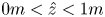 $0m<\hat {z}<1m$), for the cases: (a,d) EXP 42 with
  $(e, b, m, Re) = (0.8, 0, 0.5, 50)$; (b,e) EXP 68 with
  $(e, b, m, Re) = (0.8, 30, 0.8, {144})$; (c, f) EXP 91 with
  $(e, b, m, Re) = (0.8, 150, 0.2, {145})$. The two red dashed lines shown in each panel represent
  $\bar {C}=0.3$ and
  $\bar {C}=0.7$. The yellow dashed lines represent
  $\bar {C}=0.15$.
Focusing on figure 16(d–f), we find the region within  $\bar {C}=0.3$ and
  $\bar {C}=0.7$ appears as a fan, expanding with time for the unsteady flow. The red lines in the other two experiments remain parallel, indicating that the main front has relatively constant speed. The difference between the experiments is not obvious in the first section of the annulus, but we observe an expanding fan region between
  $\bar {C}=0.15$ and
  $\bar {C}=0.7$ in the last section of the annulus; figure 16(b), which demonstrates a severe dispersive front.
In addition to the intuitive insight into dispersion, obtained from the spatio-temporal plots, we may calculate the displacement efficiency for the three illustrative flows. Here, we calculate the efficiency of the first annular section, adopting the definition from Jung & Frigaard (Reference Jung and Frigaard2022):
 \begin{equation} \eta_{E}(\hat{t})=\frac{\displaystyle \int_{0}^{\hat{z}_{1}} \int_{{-}r_{o}}^{r_{o}}\bar{C}_x(\hat{y},\hat{z}, \hat{t})\hat{S}(\hat{y})\, {\rm d} \hat{y}\, {\rm d} \hat{z}}{\displaystyle\int_{0}^{\hat{z}_{1}} \int_{{-}r_{o}}^{r_{o}}\hat{S}(\hat{y})\, {\rm d} \hat{y}\, {\rm d} \hat{z}},\end{equation}
where  $\hat {z}_{1}$ represents the end of the first section of the annulus and
  $\bar {C}_x$ is the concentration of displacing fluid, taken from the frontal view of the annulus. The depth of the annulus in the
  $\hat {x}$-direction is denoted
  $\hat {S}(\hat {y})$, which varies with width
  $\hat {y}$. Thus, the numerator is an estimate of the volume of displacing fluids in the annulus and the denominator is the total volume of the first section. We select the same time span for comparing the three cases as they have similar flow rate, and plot the efficiency for the first section in figure 17, using the normalized experimental images. We also plot the theoretical value based on the imposed constant flow rate with red lines.

Figure 17. The efficiency  $\eta _{E}$ versus time
  $\hat {t}$ of the first section of the annulus obtained from experimental results, for the cases (a) EXP 42 with
  $(e, b, m, Re) = (0.8, 0, 0.5, 50)$; (b) EXP 68 with
  $(e, b, m, Re) = (0.8, 30, 0.8, {144})$; (c) EXP 91 with
  $(e, b, m, Re) = (0.8, 150, 0.2, {145})$. The red lines show the theoretical value based on the imposed constant flow rate.
We find a relatively good agreement between experimental and theoretical results at the initial linear stage for all three cases. The discrepancy is caused by the limitations of the pump and also from the post-processing method of the images. We observe two qualitatively different behaviours. For the unsteady flow (figure 17a), there is a smooth transition into an asymptotic regime of gradually increasing efficiency. The two steady front displacements (figure 17b,c) show an initial linear increase, corresponding to the main front passing and fairly sharp transition to a second asymptotic stage, converging to an efficiency close to 1. The discrepancy between the dispersive and non-dispersive is not clear from the efficiency plot. In general, it seems that even a moderate buoyancy force can yield a steady front flow and thus improve the efficiency. It should also be pointed out that the Reynolds number in the cases shown is relatively low, which may also help in generating a steady flow regime. We will take a further look at the effect of the Reynolds number later.
We now classify all of the  $\sim$120 experimental data points based on the flow features. As previously mentioned, the viscosity ratio
  $m$ plays a secondary role in determining the displacement type. Therefore, we disregard
  $m$ and also disregard around 30 results that have identical outcomes to those with the same buoyancy number. Moreover, if the buoyancy number and Reynolds number are held constant, we have seen that the same flow classification is observed for cases with varying eccentricities. We will therefore only consider two parameters,
  $b$ and
  $Re$, as independent variables. Approximately half of the results were easily classifiable by eye, while the other half required additional analysis using the criteria introduced earlier in the paper. Figure 18 shows the classification map of 90 experimental data. Note that each point represents five different eccentricities. We have also constructed the same classification, using both D2DGA and 3-D models, and observed a higher than 90 % coincidence rate.
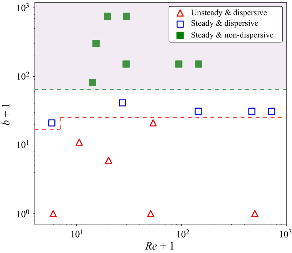
Figure 18. Overall classification of experimental results.
A clear finding is that the flows are highly dependent on the buoyancy force: higher  $b$ produces a more steady and non-dispersive regime. A boundary of
  $b\gtrapprox 80$ could delineate the non-dispersive steady front flow. There is a rather narrow region with dispersive steady front flows below this regime. Interestingly, we observe both steady and unsteady flows for the cases with the same
  $b$, i.e. an extremely low Reynolds number (
 $Re<10$) can yield a steady front flow even if the buoyant force is not sufficient to provide the steadiness. The flow starts to get highly dispersed and eventually becomes unsteady when
  $b$ is further decreased (
 $b<20$). We should mention that although the eccentricity does not seem to affect the flow regime, we still need to consider the residual fluids which cannot be distinguished directly from the front behaviour. In other words, the residual layer can be non-negligible even when the flow behaves as a non-dispersive steady front if the eccentricity is quite high.
The point here is to make a clear distinction between a steady displacement, in the sense of Pelipenko & Frigaard (Reference Pelipenko and Frigaard2004a), Carrasco-Teja et al. (Reference Carrasco-Teja, Frigaard, Seymour and Storey2008), and a steady front displacement. The former of these is a mathematical travelling wave solution that propagates along the well ensuring a fully efficient displacement. In the imperfect experimental (and numerical) arena, we need to deal with dispersion, both before and after the main displacement front. This has led to the definition of a steady front displacement for which we necessarily threshold the high and low fluid concentrations, to use (3.1). The specific threshold limits on the concentrations are evidently slightly arbitrary. Nevertheless, comparing the steady front displacements to unsteady displacements does show significant qualitative differences.
What is still missing is a clear way to quantify the behaviour of concentrations outside these thresholds. The fast moving fronts ( $w_f>1$) have resulted in dispersive metrics that appear to robustly define behaviour. The slow moving fronts are less clear, corresponding to fluid remaining on the narrow side principally. One approach to this is to define a narrow-side displacement efficiency
  $\eta _{N}$, which considers the narrowest quartile of the annulus (Maleki & Frigaard Reference Maleki and Frigaard2019; Jung & Frigaard Reference Jung and Frigaard2022). Figure 19 shows
  $\eta _{N}$ for the first section of the annulus for five non-dispersive steady front cases with different eccentricities. We also provide narrow side images for three of the cases in the inset. We find that with low or moderate eccentricity (
 $e<0.6$), the narrow-side efficiency converges to a similar high value for the different cases, due to strong secondary flow (here
  $b=150$). However, it decreases significantly if the eccentricity is sufficiently high (
 $e=0.8$), as we see in the inset image.

Figure 19. The efficiency of narrow side  $\eta _{N}$ versus time
  $\hat {t}$ of the first section of the annulus obtained from experimental results, for the cases with
  $(b, m, Re) = (150, 0.2, {145})$ and five different eccentricities (
 $e=0,0.2,0.4,0.6,0.8$). The inset shows narrow side images with three eccentricities.
4. Summary and conclusions
This paper has studied displacement flows of Newtonian fluids in a vertical eccentric annulus, from both experimental and computational aspects. Around 120 experiments have been conducted in a scaled laboratory set-up. The D2DGA and 3-D models presented by Zhang & Frigaard (Reference Zhang and Frigaard2022) have been employed to compare with experimental results. Considering the overall evolving displacement process, there is good agreement between methods on various process features: front shape, dispersion level, front velocities. This increases confidence in the accuracy and robustness of any of these methods.
A key objective of the paper was to develop criteria that help in describing the observed flow types. In models such as the 2DGA model of Bittleston et al. (Reference Bittleston, Ferguson and Frigaard2002), there is no dispersion on the scale of the annular gap. A steady travelling wave solution is mathematically possible, ensuring a perfect displacement. Moving away from steady-state displacements, azimuthal secondary flows may result in only part of the front being steady and finally the front may be fully unsteady (also a form of dispersion). For the flows considered here (experiments and more advanced models), there is always dispersion on the scale of the annulus gap. This leads us to question whether or not the flows may be steady in the meaning of Bittleston et al. (Reference Bittleston, Ferguson and Frigaard2002), when gap-scale dispersion is present?
Our analysis focused on the cross-sectionally averaged concentrations  $\bar {c}(\hat {z},\hat {t})$, as computed from either model or the experiments. Whereas our previous work in horizontal annuli showed that
  $\bar {c}$ was transported both advectively and diffusively (Renteria & Frigaard Reference Renteria and Frigaard2020), here we find that
  $\bar {c} \sim \bar {c}(\hat {z}/\hat {t})$ at long times. Vertical displacements are thus primarily advective, and the scaled front velocity
  $w_f$ can be readily computed and plotted against
  $\bar {c}$.
We begin with concentric cases ( $e=0$) to eliminate the effect of azimuthal secondary flows. We adopted a criterion from Renteria & Frigaard (Reference Renteria and Frigaard2020) to define when the front is steady: (3.1). This criterion considers the difference of normalized front velocity (
 ${\rm \Delta} w_f \le 0.1$), while ignoring the behaviour of the highest and lowest 30 % of the averaged concentration. In other words, the criterion does not address dispersion (before/after) the main front passes, nor does the criterion identify how close to the mean pumping speed the front speed is. In other words, a steady front is not the same as the steady state displacements of the 2DGA model. Not only do D2DGA and 3-D models produce the same results as experiments, insofar as (3.1) is concerned, but they are also similar in predicting the overall displacement process. Indeed the D2DGA model represents the experiments more closely that the 3-D model in some cases, especially when the buoyancy force is significant.
Having determined a robust definition for the steady/unsteady displacement front, we then addressed dispersive effects to quantify in a way that is distinct from unsteadiness. To this end, we examined the positive and negative parts of the scaled relative front velocity:  $w_{r}(\bar {c}) = w_f(\bar {c}) - 1$. We calculate the standard deviation
  $\sigma _{w_{r}^{+}}$ and the integral
  $|\bar {w}_{r}^{+}|$. The former is a measure size of the relative front velocity, i.e. dispersing ahead of the mean flow velocity. The latter represents the total dispersive volume (per unit time), for a concentric annulus. We have classified a flow as dispersive only if the conditions
  $\sigma _{w_{r}^{+}}>0.08$ and
  $|\bar {w}_{r}^{+}|>0.05$ are both met. The concentration and velocity distributions within a gap slice have also been analysed through 3-D computations, showing distinct gap-scale velocity fields related to the dispersive flows.
Using the established criteria, we classified concentric displacement flows mainly based on the buoyancy number  $b$, showing good agreement between experimental, D2DGA, and 3-D results. The flow becomes more steady as the buoyancy number
  $b$ is increased, and
  $b \sim O(10)$ is sufficient for a steady front. We find that the relative front velocity can be 10 % greater than the mean flow velocity
  $\hat {w}_0$, even at
  $b > 100$. Dispersive spikes on the gap scale are common, but the amount of dispersion can be constrained if a moderate buoyancy force is used. Specifically, flows are largely non-dispersive when
  $b>100$, as the proportion of displacing fluids with faster velocity is minimal, resulting in a small value of
  $|\bar {w}_{r}^{+}|$. For large
  $b$, the (laminar) flows we studied had limited sensitivity to either
  $Re$ or the viscosity ratio
  $m$. Some inertial effects were evident for
  $b=0$, which also was where the viscosity ratio had the clearest effect. Viscosity ratios
  $m>1$ lead to increased dispersion.
For more realistic scenarios, the annulus is eccentric. Again the data collapsed nicely to define  $w_f(\bar {c})$, indicating that with eccentricity, these vertical annulus displacements remain dominantly advective. Starting with zero buoyancy (
 $b=0$), on increasing annulus eccentricity, the fluid advances progressively further on the wide side of the annulus, leaving fluid behind on the narrow side. In general, (3.1) is not satisfied and the conditions
  $\sigma _{w_{r}^{+}}>0.08$ and
  $|\bar {w}_{r}^{+}|>0.05$ are met, indicating an unsteady dispersive flow for experiments and simulations. Considering the range of
  $\bar {c}$ for which
  $w_f<1$, we observe that the curve
  $\bar {c}(w_f)$ changes from convex to concave as
  $e$ increases. The integral
  $|\bar {w}_{r}^{-}|$ increases with
  $e$, suggesting that more of the annulus experiences residual fluids.
Surprisingly and interestingly, we find that the flow classifications do not change from those of the concentric cases. Specifically,  $b=30$ is sufficient to provide a steady front in both concentric and eccentric annuli for the fluid pairs considered. In addition, we find that the flow is in a non-dispersive regime for
  $b \approx 150$, which is similar to the concentric classification. The buoyancy force has two main roles. On one hand, it effectively restrains dispersion on the annular gap scale rather than annulus scale, regardless of the width of gap and the eccentricity of the annulus. On the other hand, a high buoyant force generates strong secondary flow: from wide side to narrow side behind the front and from the narrow side to wide side ahead of the front. Thus a relatively steady front can still be achieved even when
  $e$ is large.
However, although the displacement front behaves as steady and non-dispersive, as  $e$ increases, the amount of residual displaced fluid becomes non-negligible and is not accounted for in the above metrics or criteria. We clearly observe an increase in
  $|\bar {w}_{r}^{-}|$ with
  $e$, even when
  $b$ is large. This measure quantifies the displaced fluid that is moving slower than the mean flow velocity, and can include both slowly draining wall layers and channels of displaced fluid, typically on the narrow side. These features (mud channels and wet micro-annuli) are well known in the cementing industry and are to be avoided. However, since more extreme versions of these phenomena occur with non-Newtonian fluids, we hesitate to define a threshold on
  $|\bar {w}_{r}^{-}|$ until non-Newtonian displacement flows are considered in later studies. We have also found that
  $|\bar {w}_{r}^{-}|$ is difficult to compute accurately from the experimental data due to visualization challenges. Another drawback is that
  $|\bar {w}_{r}^{-}|$ is strongly influenced by gap-scale dispersion. We compared several steady non-dispersive cases with different eccentricities, by presenting the narrow-side displacement efficiency
  $\eta _{N}$, which considers the narrowest quartile of the annulus. We found that with low or moderate eccentricity (
 $e<0.6$), the narrow-side efficiency converges to a similar high value for the different cases, due to strong secondary flows. However,
  $\eta _{N}$ decreases significantly if the eccentricity is sufficiently high (
 $e \ge 0.8$) and may be a more robust metric to use generally.
Lastly, we presented a full classification map for all the experimental data we have obtained and discussed how design guideline for the industrial application might follow. As already mentioned, these flows are most sensitive to the buoyancy force: a greater  $b$ results in a steady front and a less dispersive regime. The novelty of the study is in accounting for dispersion separately from the steady/unsteady behaviour of the main front. Our criteria target dispersion ahead of the mean flow and appear to be robust in the sense that the two models and the experiment give consistent classifications. We need further study to better quantify dispersion/residual fluids left behind the mean flow, which is affected by large eccentricities.
We highlight here that the criteria and conclusions introduced in this paper are only strictly suitable for vertical displacements and Newtonian fluids. We have yet to apply the criteria developed to horizontal displacement flows, where we have the experiments and 3-D simulations of Renteria & Frigaard (Reference Renteria and Frigaard2020), Sarmadi et al. (Reference Sarmadi, Renteria and Frigaard2021). These flows are intuitively more dispersive but gravitational spreading induces a diffusive component to the front behaviour. The next steps in our research program on vertical displacement flows is to perform experiments with non-Newtonian fluids: mainly shear-thinning. These are closer to fluids commonly used in primary cementing displacement. In parallel, we will develop the D2DGA model for these flows.
Acknowledgements
This research has been carried out at the University of British Columbia (UBC). This research was also enabled in part by infrastructure provided from UBC Advanced Research Computing (ARC) (https://arc.ubc.ca) and Compute Canada (https://www.computecanada.ca). We thank the anonymous reviewers for their insightful comments.
Funding
Financial support for the study was provided by NSERC and Schlumberger through CRD Project No. 516022-17.
Declaration of interests
The authors report no conflicts of interest.


 Open access