


1. Introduction
Understanding animal locomotion in water, namely fish or cetacean swimming, has always attracted the attention of scientists, since the deep observations that Leonardo da Vinci described in his notes (e.g. Atlanticus Codex folio 571 A recto) more than five centuries ago. Almost two hundred years later, Borrelli, another Italian scientist, in the second half of the 17th century analysed in his book ‘De motu animalium’ the fish's motion in a very detailed manner by enhancing the essential role of the tail, as illustrated very clearly in some of his drawings.
Starting from the end of the 19th century, more systematic research has been undertaken by several zoologists, especially in England, to classify fishes in terms of tail, appendages and body movements instrumental for their propulsion. A great advance was given, in the first half of the last century, by the experimental work of Gray (Reference Gray1933), who explained for the first time the kinematics of swimming by showing the essential role of a travelling wave moving backwards along the fish's body. Starting from the above findings, Taylor (Reference Taylor1952) formulated a very successful model, now named the resistive model, well suited for swimming modes dominated by viscous forces.
On the contrary, at the start of the 1960s, Lighthill (Reference Lighthill1960) and Wu (Reference Wu1961) separately proposed a theoretical approach to study swimming modes dominated by inertial effects, i.e. for essentially inviscid flows, henceforth named the reactive model. For this purpose they considered an elongated body with a prescribed wave deformation moving from head to tail with velocity  $V$, while immersed and swimming against a stream with a constant velocity $U$ slightly lower than $V$. In a very elegant way, they predicted the power injected by the body into the surrounding fluid, the power transferred to the wake and, from the overall balance, the propulsive power required to overcome the unavoidable resistance. Essentially, the intention was to find the thrust of a deformable body by an ingenious and properly simplified formulation to allow for the evaluation of the Froude efficiency of a swimmer. Their model, described in several papers, stresses the role of the added mass as a basic mechanism for the transfer of energy to the fluid, as required for the production of the thrust and of the accompanying vortex wake.
Following their seminal work, a large number of papers appeared later on proposing many experimental techniques and numerical methods which consider a deformable body, fixed in its position in a uniform stream or tethered with the opposite velocity in a quiescent fluid. Among the experimental contributions let us mention Lauder & Tytell (Reference Lauder and Tytell2005), who provided a description of the major experimental set-ups, Tytell (Reference Tytell2004), who compared data obtained by particle image velocimetry with the estimates given by Lighthill and Wolfgang et al. (Reference Wolfgang, Anderson, Grosenbaugh, Yue and Triantafyllou1999), for the combined use of experimental and numerical results. Among the numerical contributions we recall Dong & Lu (Reference Dong and Lu2007), who reproduced for a viscous flow the conditions proposed by Lighthill and Wu, and Borazjani & Sotiropoulos (Reference Borazjani and Sotiropoulos2009), who suggested finding, for a given velocity, the equilibrium condition for self-propelled swimming. In some contributions the recoil reactions, introduced by Lighthill to satisfy the equilibrium equations for a body under a prescribed deformation, were recognized as a point of crucial importance for a correct evaluation of the swimming efficiency, see e.g. Reid et al. (Reference Reid, Hildenbrandt, Padding and Hemelrijk2012) and Maertens, Gao & Triantafyllou (Reference Maertens, Gao and Triantafyllou2017). Due to the recoil effect, the shape deformation generated by the fish for the actual locomotion gives rise to specific reactions, which modify significantly the exchanged forces and moments, hence the overall performance and the swimming trajectory. However, the procedure to obtain the full dynamics of the body under a prescribed inflow velocity is quite elaborate, hence, different routes seem more appropriate for a self-propelled locomotion.
An alternative approach in terms of centre-of-mass velocity components as unknowns of the problem was originally introduced by Saffman (Reference Saffman1967) and subsequently adopted in a seminal paper by Carling, Williams & Bowtell (Reference Carling, Williams and Bowtell1998). On the same line of reasoning, Kern & Koumoutsakos (Reference Kern and Koumoutsakos2006) extended the procedure to find optimal solutions for three-dimensional (3-D) flows and Kanso (Reference Kanso2009) obtained the locomotion variables of the swimmer‘s centre of mass by enforcing directly the conservation of the total momentum. Actually, to study a body in self-propulsion immersed in an otherwise quiescent fluid a coupled body–fluid system has to be taken into consideration with a particular attention paid to the exchange of internal forces (see Eldredge Reference Eldredge2010). Since thrust and drag counterbalance, instead of trying to calculate a propulsion power that is not easily identified (Bale et al. Reference Bale, Hao, Bhalla and Patankar2014), the Froude efficiency has to be replaced by some other measure. The cost of transport (COT), i.e. the inverse of the well-known miles per gallon adopted for cars and other vehicles (von Kármán & Gabrielli Reference von Kármán and Gabrielli1950), is given by the ratio between the expended energy and the travelled distance and becomes the proper measure in this case.
Afterwards, a very large scientific production flourished in the last decade with a focus essentially on the free-swimming COT of different species with different shape deformations and styles of swimming (see e.g. Maertens, Triantafyllou & Yue Reference Maertens, Triantafyllou and Yue2015; Borazjani & Sotiropoulos Reference Borazjani and Sotiropoulos2010). Particular attention was also paid to the efficiency parameters and to the different energy contributions spent during self-propelled swimming (Wang, Yu & Tong Reference Wang, Yu and Tong2018). A large number of papers are based on the combined solution of the deformable body dynamics and of the Navier–Stokes equations for incompressible viscous flows by different computational methods (see e.g. Yang et al. Reference Yang, Wu, Yu and Tong2008; Gazzola et al. Reference Gazzola, Chatelain, van Rees and Koumoutsakos2011; Bhalla et al. Reference Bhalla, Bale, Griffith and Patankar2013) together with under-relaxation or penalization techniques to gain the overall stability of the integration procedure. A historical survey and a comprehensive review of the most common approaches is given in several books, e.g. Webb (Reference Webb1975) and Videler (Reference Videler1993) and many review articles (e.g. Lighthill Reference Lighthill1969; Wu Reference Wu2011; Lauder Reference Lauder2015; Smits Reference Smits2019) also appeared in specific journals covering either fluid dynamics and biological aspects.
An accurate observation of the previous scientific findings, with a focus on the role of added mass and of the vorticity release, makes it easier to summarize now the main points that we like to account for when analysing self-propelled bodies:
(i) the motion of a deformable body in an infinite fluid domain is characterized by the absence of external forces and the average total momentum is conserved;
(ii) the internal forces exchanged by the swimming body with the surrounding fluid, i.e. thrust and drag, are mutually entangled, hence they are not clearly identified;
(iii) the real trajectory must account for all the recoil reactions, introduced by the prescribed deformation of the main body;
(iv) the solution of the fluid–body interaction should be solved by considering the full system of equations with the kinematic variables as output of the problem;
(v) the identification of the added mass terms leads to a naturally well-posed problem and, at the same time, provides a proper physical interpretation of the numerical results;
(vi) the standard efficiency measures are not easy to define, since the thrust is not available for steady free swimming and the COT has to be used; and
(vii) the enforced undulation is characterized by a phase velocity that is going to influence the steady state asymptotic value of the locomotion velocity and the location of the released vortices along the wake.
The purpose of the present work is to adopt a classical impulse formulation, which may be expressed in terms of potential flow and concentrated vorticity, to consider a 2-D fully immersed deformable body in the case of vanishing viscosity. The intention is to use this highly simplified impulse model with the ambitious objective to clarify the role of added mass and of vorticity release in free swimming either for the acceleration during the initial transient phase or for the asymptotic velocity to be reached at steady state.
2. Mathematical model
The self-propelled motion of an undulating body in an infinite  $N$-dimensional volume of fluid $V_\infty$ is analysed by considering a fluid–body domain with no external forces applied. Hence, the exchanged forces and moments between fluid and body appear as internal actions. The body motion is computed by solving the dynamics equations of the body centre of mass in an otherwise quiescent unbounded fluid.
With this aim, among several possible expressions for the linear and the angular momentum we adopt the classical formulation in terms of potential and vortical impulses that has been widely discussed in the literature (see e.g. Noca Reference Noca1997; Wu, Ma & Zhou Reference Wu, Ma and Zhou2015). In this framework we can easily highlight the acyclic potential contribution as well as the effects of the bound and free vorticities.
2.1. Force and moment acting on the body
The fluid momentum is expressed, via a renown vector identity (A1), by two terms representing the field vorticity and the vortex sheet over the body surface which, properly combined, readily lead to the vortical and the potential impulse. An analogous vector identity (A3) holds for the angular momentum. As has been repeatedly proven, the sum of these two impulses has the most significant property of the momentum, i.e. the forces exchanged between the body and the surrounding flow field are obtained by the time derivative of the impulses and an analogous relationship holds for the moment of the forces. At the same time, the total impulse does not suffer the poor convergence of the momentum over an unbounded domain. Actually, the momentum does not show absolute convergence, but only a conditional one. However, its finite value can be found without any ambiguity through the evaluation of the kinetic energy (see, among others, Landau & Lifschitz Reference Landau and Lifschitz1986; Childress Reference Childress2009). As a further point, the impulse formulation enjoys the important property of being linear with respect to the unknown kinematic variables, so as to permit the isolation of the potential contribution, related to the added mass characterizing fast manoeuvres, and of the vortical contribution, usually dominant when the steady state conditions are reached. We will see that this property has a paramount positive effect for the numerical solution of the equations, providing quite naturally a well-posed problem. As a final advantage, the conservation of the total impulse, peculiar to the self-propelled body, does not need the time derivation, as usually required to obtain the forces, and the successive time integration to find the kinematics of the body, providing a better accuracy together with a significant reduction of the computational effort.
We consider an impermeable, flexible body whose bounding surface  $S_b$ is moving with velocity $\boldsymbol {u}_b$ given by the prescribed deformation. We assume an incompressible fluid with density $\rho$. The outer boundary is stationary in an absolute reference frame and the fluid velocity is assumed to vanish at the far field boundary. As previously anticipated, the force acting on the body, $\boldsymbol {F}_b$, is expressed through the time derivative of the total impulse $\boldsymbol {p}$
 \begin{equation} \boldsymbol{F}_b ={-} \frac{\textrm{d} \boldsymbol{p}}{\textrm{d}t}, \end{equation}
where  ${\boldsymbol {p}}$ is defined, by using the well-known vector identity (A1) for the unbounded fluid volume, as
 \begin{equation} \boldsymbol{p} = \frac{1}{N-1} \left[ \int_{V_\infty} \rho \,{\boldsymbol{x}} \times \boldsymbol{\omega }\,\textrm{d}V +\int_{S_b} \rho \,{\boldsymbol{x}}\times (\boldsymbol{n\times u^+})\,\textrm{d}S\right], \end{equation}
where  $N = 2,3$ is the flow dimension and the integral over the external boundary receding to infinity has been proven to vanish (Noca Reference Noca1997), $\boldsymbol {\omega }$ is the vorticity and ${\boldsymbol {u^+}}$ indicates the limiting value of the fluid velocity on $S_b$. The normal to $S_b$, $\boldsymbol {n}$, points into the flow domain and all of the vorticity is enclosed within the fluid volume ${V_{\infty }}$ which extends to infinity. As shown elsewhere (Graziani & Bassanini Reference Graziani and Bassanini2002), the right-hand side of (2.2) is independent of the choice of the reference frame origin.
For a better comprehension, to account for the boundary condition on the body, which is anyhow satisfied, we may recast (2.1) by adding and subtracting a boundary integral involving  $\boldsymbol {u}_b$,
 $$\begin{gather}
\boldsymbol{F}_b ={-} \frac{\textrm{d}}{\textrm{d}t}\left\{
\frac{1}{N-1}\int_{V_{\infty}} \rho \,{\boldsymbol{x}}
\times \boldsymbol{\omega }\,\textrm{d}V
+\frac{1}{N-1}\int_{S_b} \rho \,{\boldsymbol{x}}\times
[ \boldsymbol{n} \times (\boldsymbol{u^+} -
\boldsymbol{u}_b) ]\,\textrm{d}S\right.\nonumber\\
\left. +\frac{1}{N-1}\int_{S_b} \rho
\,{\boldsymbol{x}}\times \left( \boldsymbol{n} \times
\boldsymbol{u}_b \right) \,\textrm{d}S \right\},
\end{gather}$$
$$\begin{gather}
\boldsymbol{F}_b ={-} \frac{\textrm{d}}{\textrm{d}t}\left\{
\frac{1}{N-1}\int_{V_{\infty}} \rho \,{\boldsymbol{x}}
\times \boldsymbol{\omega }\,\textrm{d}V
+\frac{1}{N-1}\int_{S_b} \rho \,{\boldsymbol{x}}\times
[ \boldsymbol{n} \times (\boldsymbol{u^+} -
\boldsymbol{u}_b) ]\,\textrm{d}S\right.\nonumber\\
\left. +\frac{1}{N-1}\int_{S_b} \rho
\,{\boldsymbol{x}}\times \left( \boldsymbol{n} \times
\boldsymbol{u}_b \right) \,\textrm{d}S \right\},
\end{gather}$$
where the jump in tangential velocity appears as a vortex sheet concentrated on the body surface to give the volume integral  $\int _{V_{\infty }} \rho \boldsymbol {x} \times \boldsymbol {\gamma } \, \textrm {d}V$, where $\boldsymbol {\gamma } = [ {\boldsymbol {n}} \times (\boldsymbol {u^+} - \boldsymbol {u}_b) ] \delta (\boldsymbol {x} - \boldsymbol {x}_b)$.
The formulation (2.3) highlights the vortex sheet term, leading to the identification of the added mass, separately from the field vorticity contribution. If, on the contrary, the total vorticity
 \begin{equation}
{\hat{\boldsymbol{\omega} }} = \boldsymbol{\omega} +
\boldsymbol{\gamma} = \boldsymbol{\omega} + [
{\boldsymbol{n}} \times (\boldsymbol{u^+} -
\boldsymbol{u}_b) ] \delta (\boldsymbol{x} -
\boldsymbol{x}_b),
\end{equation}
\begin{equation}
{\hat{\boldsymbol{\omega} }} = \boldsymbol{\omega} +
\boldsymbol{\gamma} = \boldsymbol{\omega} + [
{\boldsymbol{n}} \times (\boldsymbol{u^+} -
\boldsymbol{u}_b) ] \delta (\boldsymbol{x} -
\boldsymbol{x}_b),
\end{equation}is considered, the added mass would be embedded and fully hidden within the field vorticity, as discussed by Limacher, Morton & Wood (Reference Limacher, Morton and Wood2018).
Similarly to what is described above for the force, an expression for the angular moment (positive anticlockwise) on the body can be obtained. Here, we consider the moment with respect to a given pole (to be specified later either as the origin of the ground reference frame or as the body centre of mass), so  $\boldsymbol {x}$ is the generic distance of the field point from the pole.
By defining the angular impulse  $\boldsymbol {{\rm \pi} }$ as:
 \begin{equation} \boldsymbol{\rm \pi} ={-} \tfrac{1}{2} \left[ \int_{V} \rho \,{|x|}^2 \boldsymbol{\omega} \, \textrm{d}V + \int_{S_b} \rho \,{|x|}^2 (\boldsymbol n \times \boldsymbol u^+ ) \, \textrm{d}S \right], \end{equation}
the expression for the angular moment is written as
 \begin{equation} \boldsymbol{M}_b ={-} \frac{\textrm{d}\boldsymbol{\rm \pi}}{\textrm{d}t}. \end{equation}
2.2. Potential and vortical impulse
A Helmholtz decomposition is applied to express the velocity field as the sum of the acyclic and vorticity related components
 \begin{equation} \boldsymbol{u^+} = \boldsymbol{\nabla} \phi + \boldsymbol{\nabla} \times \boldsymbol{\varPsi} = \boldsymbol{\nabla} \phi + \boldsymbol{u}_w, \end{equation}
where  $\phi$ and $\boldsymbol {\varPsi }$ are referred to as the scalar and the (solenoidal) vector potentials, and are given by the solution of the Laplace/Poisson equation, subject to the impermeable boundary condition on $S_b$, i.e. $\boldsymbol {\nabla } \phi \boldsymbol {\cdot } \boldsymbol {n} = \boldsymbol {u}_b \boldsymbol {\cdot } \boldsymbol {n}$ and $(\boldsymbol {\nabla } \times \boldsymbol {\varPsi })\boldsymbol {\cdot } \boldsymbol {n} = 0$ respectively, and to the vanishing velocity at infinity. To enlighten the contribution of the above potentials to the force, let us now express the impulse $\boldsymbol {p}$ appearing in (2.1) in terms of both potential and vortical impulses, $\boldsymbol {p}_{\phi }$ and $\boldsymbol {p}_{v}$, as
 \begin{equation} \boldsymbol{p} = \boldsymbol{p}_\phi + \boldsymbol{p}_v. \end{equation}
The vortical impulse on the right hand-side of (2.8) is
 \begin{align} \boldsymbol{p}_v = \frac{1}{N-1} \left[ \int_{V_{\infty}}\rho \; {\boldsymbol{x}} \times \boldsymbol{\omega}\,\textrm{d}V + \int_{S_b }\rho \; {\boldsymbol{x}}\times (\boldsymbol{n} \times \boldsymbol{u}_w) \, \textrm{d}S \right] = \frac{1}{N-1} \int_{V_{\infty}}\rho \; {\boldsymbol{x}} \,\times \,\boldsymbol{\omega}_a\,\textrm{d}V, \end{align}
where part of the bound vorticity on  $S_b$ has been added to the released vorticity to obtain the additional vorticity as introduced by Lighthill
 \begin{equation} {\boldsymbol{\omega}_a} = {\boldsymbol{\omega}} + ({\boldsymbol{n}} \times \boldsymbol{u}_w) \,\delta (\boldsymbol{x} - \boldsymbol{x}_b) \end{equation}
that may be expressed, once combined with (2.4), to reproduce the original definition
 \begin{equation} {\boldsymbol{\omega}_a} = {\hat{\boldsymbol{\omega} }} - \left[ {\boldsymbol{n}} \times (\boldsymbol{\nabla} \phi - \boldsymbol {u}_b) \right] \,\delta (\boldsymbol{x} - \boldsymbol{x}_b). \end{equation}
The potential impulse  $\boldsymbol {p}_\phi$ on the right hand-side in (2.8) is given by
 \begin{equation} \boldsymbol{p}_\phi ={-} \rho \; \int_{S_b} \phi\, {\boldsymbol{n}} \, \textrm{d}S, \end{equation}
where the vector identity (A2) has been used. Let us notice that this term has been named also the virtual momentum by Saffman (Reference Saffman1992) or impulse of the fluid by Lamb (Reference Lamb1975) and its time derivative defines, in a general sense, the added mass force that, for rigid motions, may be expressed in the classical form given by the Kirchhoff base potentials.
The expression for the angular momentum can be similarly obtained by separating the vortical and the potential contributions by using the vector identity (A3) and the generalized Stokes theorem (A4). We split the angular impulse (2.5) as  ${\boldsymbol {{\rm \pi} }} = {\boldsymbol {{\rm \pi} }}_\phi + {\boldsymbol {{\rm \pi} }}_v$, where the angular potential impulse is defined as
 \begin{equation} {\boldsymbol{\rm \pi}}_\phi ={-}\tfrac{1}{2} \int_{S_b} \rho \, {|x|}^2 (\boldsymbol n \times \boldsymbol{\nabla} \phi) \, \textrm{d}S ={-} \rho \, \int_{S_b} \boldsymbol x \times \phi \boldsymbol n \, \textrm{d}S, \end{equation}
and the angular vortical impulse is
 \begin{equation} {\boldsymbol{\rm \pi}}_v ={-}\tfrac{1}{2} \int_{V} \rho \, {|x|}^2 \boldsymbol{\omega} \, \textrm{d}V -\tfrac{1}{2} \int_{S_b} \rho \, {|x|}^2 (\boldsymbol n \times \boldsymbol {u}_w ) \, \textrm{d}S. \end{equation}
As a comment to this section, a unified theoretical treatment of the impulse formulation has been presented by taking into account the main different contributions on the subject (see e.g. Saffman Reference Saffman1967; Kanso Reference Kanso2009; Eldredge Reference Eldredge2010). Concerning the vorticity field, particular attention is paid to the bound vorticity and to its relationship with the added mass force (see e.g. Lighthill Reference Lighthill1960; Limacher Reference Limacher2019).
3. Locomotion
We study now the planar motion of a deformable body  $\mathcal {B}$ within an infinite fluid domain $\mathcal {V}$. We use a Cartesian inertial frame $(\boldsymbol {e}_1, \boldsymbol {e}_2, \boldsymbol {e}_3)$. The body motion occurs in the plane $(\boldsymbol {e}_1, \boldsymbol {e}_2)$ and its translation with respect to a given reference point in $\mathcal {B}$ is $\boldsymbol {x}_o = x_o \, \boldsymbol {e}_1 + y_o \, \boldsymbol {e}_2$. Moreover, the body may undergo a rotation $\beta$ about the axis $\boldsymbol {e}_3$.
The locomotion of the deformable body is obtained by coupling the body dynamics and the fluid dynamics actions. If we consider the body–fluid system ( ${{\mathcal {V}}_b} + {{\mathcal {V}}_f}$), no external forces or moments are present and therefore the linear and angular momenta are conserved
 \begin{gather} \frac{\textrm{d}}{\textrm{d}t} \left[ \int_{{\mathcal{V}}_b} \rho_b \, \boldsymbol {u}_b \, \textrm{d}V + \int_{{\mathcal{V}}_f} \rho \, \boldsymbol u \, \textrm{d}V \right] = 0, \end{gather}
 \begin{gather} \frac{\textrm{d}}{\textrm{d}t} \left[ \int_{{\mathcal{V}}_b} \rho_b \, \boldsymbol x \times \boldsymbol {u}_b \, \textrm{d}V + \int_{{\mathcal{V}}_f} \rho \, \boldsymbol{x} \times \boldsymbol u \, \textrm{d}V \right] = 0. \end{gather}
 The motion of the body can be expressed as the sum of the prescribed deformation (shape variations with velocity  $\boldsymbol {u}_{sh}$) plus the motion of the frame with origin in the centre of mass (translational, $\boldsymbol {u}_{\rm cm}$, and rotational, $\boldsymbol \varOmega$, velocity).
In the ground inertial frame the angular velocity is  $\boldsymbol {\varOmega } = \dot \beta \, \boldsymbol {e}_3 \equiv {\varOmega } \, \boldsymbol {e}_3$. The linear velocity is $\boldsymbol {u}_{\rm cm} = \dot {x}_o \boldsymbol {e}_1 + \dot {y}_o \boldsymbol {e}_2$. Thus we can express the body motion as
 \begin{equation} \boldsymbol {u}_b = \boldsymbol {u}_{sh} + \boldsymbol {u}_{\rm cm} + \boldsymbol{\varOmega} \times \boldsymbol x^\prime, \end{equation}
where  $\boldsymbol x^\prime$ is the position vector in the body frame, i.e. $\boldsymbol x = \boldsymbol {x}_{\rm cm} + \boldsymbol x^\prime$. Following (3.3), the prescribed deformation of the body has to conserve linear and angular momenta
 \begin{gather} \int_{{\mathcal{V}}_b} \rho_b \boldsymbol {u}_{sh} \, \textrm{d}V = 0, \end{gather}
 \begin{gather} \int_{{\mathcal{V}}_b} \rho_b \boldsymbol x^\prime \times \boldsymbol {u}_{sh} \, \textrm{d}V = 0. \end{gather}
By considering that the second term in (3.1) is the force acting on the fluid, which is opposite to the force on the body and by using the body mass  $m_b$, combining with (2.1) we obtain
 \begin{equation} \frac{\textrm{d}}{\textrm{d}t} ( m_b \, \boldsymbol {u}_{\rm cm}) + \frac{\textrm{d} \boldsymbol{p}}{\textrm{d}t} = 0, \end{equation}
where  $\boldsymbol {u}_{\rm cm}$ is clearly identified as the locomotion velocity of the body and $\boldsymbol p$ is now expressed in terms of $\boldsymbol x^\prime$, since the independence on the origin of the reference system. In this way, the interaction with the fluid gives directly the full motion of the undulating body. Otherwise, if ((3.4)–(3.5)) were not satisfied by the prescribed deformation, additional rigid motions would appear and (3.3) should be consistently modified (see Bhalla et al. Reference Bhalla, Bale, Griffith and Patankar2013). By assuming zero initial conditions (3.6) gives
 \begin{equation} m_b \, \boldsymbol{u}_{\rm cm} + \boldsymbol{p} = 0. \end{equation}
 Similarly, the angular impulse in two dimensions is recast from (2.5) in terms of the distance  $\boldsymbol {x^\prime }$ as ${\rm \pi} ^\prime = (\boldsymbol {{\rm \pi} } - \boldsymbol {x}_o \times \boldsymbol p)\boldsymbol {\cdot }\boldsymbol {e}_3$ and the angular momentum balance can be expressed as
 \begin{equation} \frac{\textrm{d}}{\textrm{d}t} ( I_{zz} \, \varOmega ) + \frac{\textrm{d} \boldsymbol {\rm \pi}^\prime}{\textrm{d}t} = 0, \end{equation}
or, by using the body frame and removing the time derivative
 \begin{equation} I_{zz} \, \varOmega + {{\rm \pi}^\prime} = 0 . \end{equation}
 In the case of a massless body ( $m_b =0$ and $I_{zz} =0$) we recover the equations reported by Kanso (Reference Kanso2009). Let us notice that, according to what was originally proposed by Saffman (Reference Saffman1967), the system of (3.7) and (3.9) provides the evaluation of the body velocities without considering time derivatives, as required when using the standard equations (3.6) and (3.8).
The scalar potential introduced by the Helmholtz decomposition is further divided as  $\phi = \phi _{sh} + \phi _{loc}$, as suggested by Saffman (Reference Saffman1967), where $\phi _{sh}$ is given by the imposed deformation velocity $\boldsymbol {u}_{sh}$ and $\phi _{loc}$ is given by the combination of the locomotion linear and angular velocities, according to the related boundary conditions on $S_b$
$S_b$
 \begin{equation} \frac{\partial\phi_{sh}}{\partial n} = \boldsymbol{u}_{sh} \boldsymbol{\cdot} \boldsymbol{n},\quad \frac{\partial\phi_{loc}}{\partial n} = (\boldsymbol{u}_{\rm cm} + \boldsymbol{\varOmega}\times\boldsymbol{x}^\prime) \boldsymbol{\cdot} \boldsymbol{n}. \end{equation}
Analogously, the linear and angular impulses are given by
 \begin{equation} \boldsymbol{p}_{\phi} = \boldsymbol{p}_{sh} + \boldsymbol{p}_{loc},\quad {{\rm \pi}^\prime_{\phi}} = {{\rm \pi}^\prime_{sh}} + {{\rm \pi}^\prime_{loc}}. \end{equation}
 Finally, the locomotion impulses,  $\boldsymbol {p}_{loc}$ and ${{\rm \pi} ^\prime _{loc}}$, may be expressed in terms of the added mass coefficients reported in the classical treatises (see e.g. Lamb Reference Lamb1975) that, for completeness, are briefly recalled below. For a body motion with linear velocity $\boldsymbol {u}_{\rm cm}$ and angular velocity $\varOmega$, we consider the Kirchhoff base potentials $\varPhi _j$ defined through the boundary conditions
 \begin{equation} \frac{\partial\varPhi_1}{\partial n} = \boldsymbol{n}\boldsymbol{\cdot}\boldsymbol{e}_1,\quad \frac{\partial\varPhi_2}{\partial n} = \boldsymbol{n}\boldsymbol{\cdot}\boldsymbol{e}_2,\quad \frac{\partial\varPhi_3}{\partial n} = \boldsymbol{x}^\prime\times\boldsymbol{n}\boldsymbol{\cdot}\boldsymbol{e}_3 \end{equation}
to have  $\phi _{loc} = \dot {x}_0 \varPhi _1 + \dot {y}_0 \varPhi _2 + \varOmega \varPhi _3$. It follows for the added mass coefficient $m_{ij}$ that
 \begin{equation} m_{ij} = \rho \int_{S_b} \varPhi_i \, \frac{\partial \varPhi_j}{\partial n} \, \textrm{d}S. \end{equation}
 To compute the numerical solution we express the locomotion equations in a coordinate frame attached to the body. For this purpose we consider the ground fixed frame  $\{{ \boldsymbol {e}_1, \boldsymbol {e}_2,\boldsymbol {e}_3 }\}$ and the body frame $\{{ \boldsymbol {b}_1, \boldsymbol {b}_2,\boldsymbol {b}_3 }\}$ as sketched in figure 1. The origin of the body frame is in cm, i.e. $\boldsymbol {x}_o \equiv \boldsymbol {x}_{\rm cm}$ and $\boldsymbol {b}_3$ is parallel to $\boldsymbol {e}_3$. Accordingly, the linear velocity $\boldsymbol {V}_{\rm cm} = V_1 \, \boldsymbol {b}_1 + V_2 \, \boldsymbol {b}_2$ and the momenta $\boldsymbol {P}$, $\varPi$ are related to the corresponding variables in the fixed frame by
 \begin{equation} \boldsymbol{u}_{\rm cm} = \boldsymbol{R} \, \boldsymbol{V}_{\rm cm},\quad \boldsymbol{p} = \boldsymbol{R} \, \boldsymbol{P}, \quad \boldsymbol{\rm \pi}^\prime = {\varPi}, \end{equation}
where  $\boldsymbol {R}$ is the rotation matrix relating the inertial to the body frame. Analogously, the coordinates in the body frame are $\boldsymbol X = \boldsymbol R^T \; \boldsymbol x^\prime$.

Figure 1. Ground and body reference frames.
Accounting for (3.14a–c), the impulses related to the body deformation,  $\boldsymbol {P}_{sh}$ and $\varPi _{sh}$, are expressed according to (2.12) and (2.13), respectively, while the vorticity related quantities, $\boldsymbol {P}_{v}$ and $\varPi _{v}$, are defined through (2.9) and (2.14). The locomotion velocities, which are multiplied by the added mass coefficients (3.13) within $\boldsymbol {P}_{loc}$ and $\varPi _{loc}$, can be shifted to the left hand-side to yield the system of equations for the body motion
 \begin{equation} \left. \begin{aligned} V_1 \, \left(m_{11} - {m_b} \right) + V_2 \, m_{12} + \varOmega \, m_{13} & = {{P}_{sh}}_1 + {P_{v}}_1, \\ V_1 \, m_{21} + V_2 \, \left(m_{22} - {m_b} \right) + \varOmega \, m_{23} & = {{P}_{sh}}_2 + {P_{v}}_2, \\ V_1 \, m_{31} + V_2 \, m_{32} + \varOmega \left( m_{33} - {I_{zz}} \right) & = \varPi_{sh} + \varPi_{v}. \end{aligned} \right\} \end{equation}
 The added mass terms, appearing on the left hand-side of (3.15), together with the body inertial properties, give the coefficient matrix for the unknown variables  $V_1$, $V_2$ and $\varOmega$. The known terms appearing on the right hand-side are the impulse contributions due to shape deformation and vorticity. This equation system recalls and generalizes the model ingeniously proposed by Saffman (Reference Saffman1967) and Lighthill (Reference Lighthill1970). The body mass $m_b$ is assumed to be constant while $I_{zz}$ and $m_{ij}$ change in time according to the shape deformation. Let us stress again that the part of the added mass terms related to $\phi _{loc}$ now appears on the left-hand side, leading to a well-posed problem, as briefly described in the following section together with the main details of the numerical model. The separation of $\phi _{sh}$ and $\phi _{loc}$ is also instrumental to identifying the exchange of added mass energy among shape deformation and locomotion (see Spagnolie & Shelley Reference Spagnolie and Shelley2009; Steele Reference Steele2016). We would like to underline that the part of the potential impulses related to $\phi _{sh}$ in (3.15), as suggested by Kanso (Reference Kanso2009), has to stay on the right hand-side together with the vortical impulses, since they both involve known quantities. As a further comment, a detailed account of the single contributions is the essential tool for arguing about the aim of the paper, i.e. a proper evaluation of the role of added mass and vorticity release when discussing the numerical results.
4. About the numerical model
The mathematical model described so far is valid in general although, from now on, restricted to the locomotion of 2-D bodies to facilitate the analysis of the results while maintaining the most important aspects of the problem. As a further step in the same direction, we consider here an accurate but simplified numerical model which does not involve vorticity diffusion, in the way suggested by Schultz & Webb (Reference Schultz and Webb2002), to find sufficiently accurate results for this complicated problem. The evaluation of both potential and vortical impulses can be obtained by the discretization of the body surface and by a suitable model for the release of the concentrated vortex sheet via a Kutta condition to mimic the presence of a vanishing viscosity. Some of the techniques adopted in the numerical method for the evaluation of the two impulses are briefly described below, but we would like to illustrate first the capability of the present model to provide a well-posed linear system.
Actually, the time derivatives, usually needed with the classical pressure formulation, may lead to a poor stability of the equation system, since the forces and moments are directly dependent on the unknown velocity components. Some authors, e.g. Carling et al. (Reference Carling, Williams and Bowtell1998), Kern & Koumoutsakos (Reference Kern and Koumoutsakos2006) and Borazjani & Sotiropoulos (Reference Borazjani and Sotiropoulos2010), tried to overcome these difficulties by using under-relaxation expressions which had to be accurately chosen to obtain stability and to minimize their influence on the numerical accuracy of the procedure. A more physical approach was adopted in Maertens et al. (Reference Maertens, Gao and Triantafyllou2017) by introducing a prescribed added mass matrix  $\boldsymbol {M}_a$, whose coefficients are estimated and properly tuned from the stretched straight configuration. By adding to both sides of the equation the same term representing this approximated value, the idea is to counterbalance the real added mass embedded within the forcing term. The impulse formulation adopted here allows for the removal of the time derivatives present in (3.6) and (3.8), hence no stability issues should be considered. At the same time, the linearity of the vorticity terms allows us to isolate and separate the contribution of the added mass, which is correctly evaluated at each time step and properly moved to the left hand-side, giving a well-posed system of equations able to hold even when treating massless bodies (see Eldredge Reference Eldredge2010).
To achieve neat and simple results, as anticipated above, we consider the case of potential flow with a concentrated vorticity on the body surface and its subsequent shedding at the trailing edge into the vortex wake. The flow solutions are obtained by using an unsteady potential code based on the approach of Hess & Smith (Reference Hess and Smith1967) while the wake release is taken into account by following the procedure described in Basu & Hancock (Reference Basu and Hancock1978). The body boundary is approximated by a finite number of panels, each with a local, uniform source strength, and all with a constant circulation density. The impermeability condition on each panel together with a suitable unsteady Kutta condition are needed to evaluate the source strengths and the uniform circulation density  $\gamma$. According to Kelvin's theorem, any change in circulation about the airfoil results in the release of vorticity by a wake panel attached to the trailing edge which, at each time step, is lumped into a point vortex and shed into the wake.
As described in the previous section, even if the equations are written in the ground frame of reference, the solution is achieved in a coordinate system attached to the body which moves according to  $V_1$ and $V_2$ and rotates according to $\varOmega$. Actually, this is the proper frame to define the deformation which should not be dependent on the interaction with the fluid. At each time step, the body, deforming with $\boldsymbol {V}_{sh}$, is invested with a water speed given by the combination of $-V_1$, $-V_2$ and $-\varOmega$, which is required for the unsteady Kutta condition and it is essential for the evaluation of the length and inclination of the wake panel behind the body through several iterations.
Finally, it is important to notice that the linear velocity components  $V_1$ and
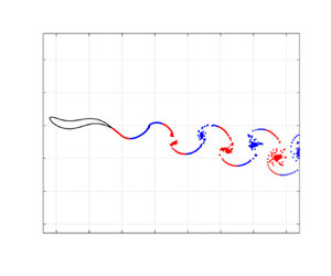
  $V_2$, named, from now on, the forward and lateral velocities, respectively, change their directions at each time step, since the equations of motion are written in the body frame coordinates. After a transient acceleration phase, the body, even maintaining an oscillating pattern, reaches an asymptotic steady state with a constant mean value of the forward velocity while the mean lateral and angular velocities are equal to zero. As a consequence, in the following section, the numerical results are shown in terms of the forward velocity, whose mean value represents the actual locomotion velocity. An animation showing the body motion, obtained by projecting the velocity components $V_1$ and $V_2$ along the $x$ and $y$ directions of the ground frame of reference (animation-link), is helpful to better illustrate the actual gait of the body. As a final comment, the above numerical model may be considered as part of the splitting procedure introduced by Chorin (Reference Chorin1973) which, accounting for diffusive vorticity, leads directly to the classical vortex method for viscous flow (see e.g. Graziani, Ranucci & Piva Reference Graziani, Ranucci and Piva1995; Koumoutsakos & Leonard Reference Koumoutsakos and Leonard1995; Eldredge, Colonius & Leonard Reference Eldredge, Colonius and Leonard2002).
5. Numerical results and discussion
We would like to analyse in the present section the free swimming of a deformable body with a focus on the asymptotic steady state condition. The fish undulates with a prescribed periodic deformation characterized by a specific phase velocity and, after a transient, the fish reaches a steady state under the combination of potential and vortical velocity contributions. Let us note that the resulting value depends only on the phase velocity while the single contributions may vary with the deformation amplitude. As anticipated in the previous sections, the standard efficiency measures are not suitable, while the present results provide the data needed for the evaluation of the cost of transport. As a further point, the results allow for interesting considerations of the transient phases, which are also illustrated through the representation of the wake patterns.
5.1. Body shape and kinematics
The swimming fish at rest is represented by a shape corresponding to a NACA $0012$ airfoil with a chord length $c$ equal to $1$. Previous works employed a large number of different approaches to describe fish undulation. Some of the proposed analytical expressions for the lateral displacement of the mid-line were obtained by fitting data from direct fish observations (see e.g. Hess & Videler Reference Hess and Videler1984; Lauder & Tytell Reference Lauder and Tytell2005). These analytical expressions consist of a travelling wave usually multiplied by a polynomial amplitude modulation, thus allowing for direct control of geometrical parameters, such as the tail-beat amplitude. An additional mathematical condition is required to enforce the inextensibility given by
 \begin{equation} \left(\frac{\partial y_c}{\partial s}\right)^2 + \left(\frac{\partial x_c}{\partial s}\right)^2 = 1, \end{equation}
where  $x_c$ and $y_c$ are the mid-line coordinates and $s$ represents the curvilinear coordinate along the mid-line itself. To satisfy implicitly this condition, some authors proposed a deformation in terms of the mid-line curvature from which the lateral displacement follows (Kern & Koumoutsakos Reference Kern and Koumoutsakos2006; Wang et al. Reference Wang, Yu and Tong2018).
Here, a different parameterization based on the instantaneous local slope of the mid-line is proposed as more affordable for bio-mimetic applications, hereafter referred to as synthetic deformation. The slope of the mid-line is defined by the following expression for a travelling wave of constant amplitude  $d\beta$ and a wavenumber $k$ related to a wavelength along $s$
$s$
 \begin{equation} \beta(s,t) = d\beta\sin(k s - \omega t), \end{equation}
where  $\omega$ is the angular frequency. An amplitude modulation may eventually be added to reproduce the deformations given by other authors. The instantaneous coordinates of the airfoil mid-line are obtained by integrating (5.2)
 \begin{gather} x_c(s,t) = \int_0^s \cos\left(\beta(s,t)\right)\,\textrm{d}s, \end{gather}
 \begin{gather} y_c(s,t) = \int_0^s \sin\left(\beta(s,t)\right)\,\textrm{d}s, \end{gather}
and the inextensibility condition is automatically satisfied. The normal to each cross-section of the body is the same as that of the mid-line and the total area is preserved at convergence during the deformation.
In the absence of surrounding fluid, namely, with no external forces and moments, (3.4) and (3.5) hold to maintain the centre of mass position of the body, as well as its principal axes (figure 2a). If these equations are not satisfied, the centre of mass would move under spurious forces (figure 2b), hence, the deformation has to be properly corrected by removing the rigid displacements so to obtain the mid-line envelope in figure 2(a).

5.2. Swimming velocity and expended energy
The present section contains the results for a neutrally buoyant ( $\rho = \rho _b/\rho _f = 1$) body undulating with a fixed angular frequency $\omega = 2{\rm \pi} f = 10\ \textrm {rad}\,\textrm {s}^{-1}$, unless otherwise indicated. For all the analysed cases, the wavenumber $k$ is set to $2{\rm \pi} \ \textrm {m}^{-1}$, i.e. the wavelength $\lambda$ is equal to the chord length $c$, hence corresponding to a phase speed which, according to (5.2), is given by
 \begin{equation} \frac{\omega}{k} = f \lambda = 1.59\ \textrm{m}\,\textrm{s}^{{-}1}. \end{equation}
The forward locomotion velocity component  $U$ is shown in figure 3 for different deformation amplitudes $\delta \beta$. By increasing $\delta \beta$, we notice larger transient acceleration and a steady state velocity that is slightly decreasing. However, due to the inextensibility condition, the wavelength $L$, associated with the instantaneous deformation and measured along the forward direction (see figure 4) may be quite different from the prescribed $\lambda$. From this observation, an equivalent wavelength $\lambda _e$ is defined as
 \begin{equation} \lambda_e = \frac{1}{T}\int_{t}^{t+T}L(t)\,\textrm{d}t, \end{equation}
which leads to an equivalent phase velocity of the body deformation given by
 \begin{equation} \frac{\omega}{k_e} = f\lambda_e. \end{equation}
As a consequence, the asymptotic value of the slip velocity, defined as the ratio between the swimming speed and the equivalent phase velocity, does not change with  $d\beta$, as shown in figure 5, namely, the body moves with a forward velocity which only depends on the backward travelling wave velocity, and not on its amplitude. Since the model does not consider any dissipative effect, the above result seems reasonable, while, under the action of viscous resistance, the slip velocity would definitely be lower and the deformation amplitude would start to play a significant role (Smits Reference Smits2019). For comparison, we report in figure 6 the results for the velocity components for the present model and a carangiform deformation together with those for the viscous model by Yang et al. (Reference Yang, Wu, Yu and Tong2008). The figure confirms that the main effect of the viscous resistance is a consistent reduction of the steady state locomotion velocity which may otherwise be predicted by introducing a model approximation for the viscous drag (see e.g. Akoz & Moored Reference Akoz and Moored2018). In this case, numerical results not reported here reproduce an increasing trend of the asymptotic swimming velocity with the deformation amplitude, as shown by analogous findings in the literature (e.g. Zhang et al. Reference Zhang, Pan, Chao and Yan2018).

Figure 3. Forward swimming velocity for different undulation amplitudes.

Figure 4. Equivalent wavelength  $\lambda _e$.

Figure 5. Slip velocity for different undulation amplitudes.

Figure 6. Velocity components ( $U, V, \varOmega$) for carangiform deformation: present vs viscous results (Yang et al. Reference Yang, Wu, Yu and Tong2008).
As discussed previously, the effects of added mass and vorticity release on the swimming speed may be easily highlighted. Actually, due to the linearity of the system of (3.15), the kinematic variables  $U$,
$U$,  $V$ and $\varOmega$ are given by adding the potential and the vortical impulses. The corresponding forward velocity contributions, $U_\phi$ and $U_w$, are illustrated in figures 7(a) and 7(b) in the form of the slip velocity. For growing amplitude, $U_\phi /(f\lambda _e)$ increases and $U_w/(f\lambda _e)$ decreases and their sum remains constant, as anticipated in figure 5. Let us observe that $U_\phi$, due to the added mass, reaches instantaneously a steady state value, and $U_w$, due to vortex shedding, grows in time with a certain delay. At the same time, it is worth stressing that the rate of change of $U_w$ in the transient is deeply related to the pure potential impulses since a larger added mass contribution induces a larger acceleration and a more intense vortex shedding, as shown in figure 8 and firmly stated by Limacher et al. (Reference Limacher, Morton and Wood2018). From the above considerations, we can deduce that, for conditions usually adopted for efficient cruising at steady state, we should reduce $U_\phi$, hence the contribution due to $\boldsymbol {p}_{sh}$ and $\boldsymbol {{\rm \pi} }_{sh}$, to have a lower intensity of the released vortices. In these conditions, the total velocity is essentially given by $U_w$, which may reach a large value although maintaining a weak vortex shedding. On the contrary, a large $U_\phi$ contribution is required in escape manoeuvres such as a C-start to give the initial instantaneous burst together with a larger acceleration accompanied by a larger energy consumption, as discussed below, which, however, is not a priority in this case. The following vortical contribution becomes eventually predominant at the end of the C-start manoeuvre, in a way analogous to, but more pronounced than, the steady swimming results.

Figure 7. Forward component of the slip velocity for  $\rho = 1$ and different undulation amplitudes: (a) potential contributions; (b) vorticity contributions

Figure 8. Released circulation for different undulation amplitudes.
At this point, looking at figure 5, we observe that the steady state velocity does not match the phase velocity and the following question arises: Why does the slip velocity differ from one? Actually, the wave phase velocity generated by the body and transferred to the fluid appears to depend on the whole motion of the body, i.e. prescribed undulation plus recoil. To verify the above observation, it is helpful to consider a well-established analytical model which may allow for a better understanding of the obtained results. More specifically, the elongated body theory (Lighthill Reference Lighthill1960) provides an analytical expression to evaluate the time averaged thrust exerted on an undulating body by a fluid with an assigned uniform velocity  $U$ and a given lateral displacement $h(x,t)$
 \begin{equation} \bar{T} = \frac{1}{2}\rho_fA(L)\left[\overline{\left(\frac{\partial h}{\partial t}\right)^2} - U^2 \overline{\left(\frac{\partial h}{\partial x}\right)^2}\right]_{x=L}, \end{equation}
where  $A(L)$ is the added mass associated with the trailing edge of the body and the overline indicates a mean value over time. Afterwards, Lighthill introduced the concept of recoil associated with the displacement $h$, in terms of lateral and angular rigid motions that must be added to $h$ in order to respect the corresponding equilibrium equations. For the sake of conciseness, only the equation for the lateral momentum balance is reported here
 \begin{equation} \rho_b\int_0^L S(x)\frac{\partial^2h}{\partial t^2}\,{\textrm{d}\kern0.05em x} ={-}\rho_f\int_0^L \left(\frac{\partial}{\partial t} + U\frac{\partial}{\partial x}\right)\left[A(x)\left(\frac{\partial h}{\partial t} + U\frac{\partial h}{\partial x}\right) \right]\, {\textrm{d}x}, \end{equation}
where  $S(x)$ is the cross-sectional area of the elongated body and $A(x)$ is the related added mass.
By introducing a travelling wave  $\tilde {h}$ with phase velocity ${\omega }/{k}$ and amplitude $a$, i.e.
 \begin{equation} \tilde{h}(x,t) = a\sin\left(kx-\omega t\right), \end{equation}
it is easy to show that zero thrust in (5.8) can be achieved if the velocity  $U$ is equal to the phase velocity. In fact, assuming $U = {\omega }/{k}$, the right-hand side of (5.9) is always equal to zero for the wave kinematic condition
 \begin{equation} \frac{\partial \tilde{h}}{\partial t} + \frac{\omega}{k}\frac{\partial \tilde{h}}{\partial x} = 0, \end{equation}
while the left-hand side is different from zero, unless particular choice is made for  $S(x)$, i.e. the shape of the body. Hence, in principle, $\tilde {h}$ should be modified by taking into account the recoil motions $B(x,t)$ (see e.g. Singh & Pedley Reference Singh and Pedley2008)
 \begin{equation} h(x,t) = \tilde{h}(x,t) + B(x,t). \end{equation}
When the recoil is added to the original undulation, the total motion  $h$ no longer annihilates the thrust (5.8) for $U = {\omega }/{k}$, but either a rigid translation and/or a rotation motion modifies the asymptotic velocity as
 \begin{equation} U = \chi \frac{\omega}{k}, \end{equation}
where the factor  $\chi$, which can be evaluated by a very simple approximation, is larger than one for the present case. As a further assessment, let us notice that (5.9) is directly satisfied by $\tilde {h}$ when $\rho _b$, appearing on the left-hand side, is equal to zero, i.e. when a massless body is considered (see Kanso Reference Kanso2009). It follows that, in these conditions, no recoil motion occurs and the asymptotic velocity $U$ is always equal to ${\omega }/{k}$. In fact, a massless body is able to achieve the same forward speed as that of the fluid pushed backwards by the travelling wave since, in principle, the presence of the body is only attested by its virtual mass given by the surrounding fluid. If we extend the above reasoning, valid for the undulating body in a uniform stream, to the case of self-propelled locomotion, the same conclusion may be reached for the mean force in the forward direction, whose value tends to vanish at steady state conditions.
The just mentioned influence of the recoil on a prescribed deformation may be of great interest also for different phenomena related to swimming control means. For instance, by looking at (3.15) we may see how all the velocity components may substantially vary with the added mass coefficient  $m_{ij}$, as perceived by certain types of fish able to change their configuration during a predator–prey interaction, as done by the sailfish by raising its dorsal fin (see Paniccia et al. Reference Paniccia, Graziani, Lugni and Piva2021).
From an energy point of view, an intense vortex shedding results in a high consumption in terms of kinetic energy released into the flow field, as shown by figure 9. The fluid kinetic energy is obtained (see Graziani et al. Reference Graziani, Ranucci and Piva1995; Kanso Reference Kanso2009) as
 \begin{equation} E = \frac{1}{2}\int_S\phi\frac{\partial\phi}{\partial n}\,\textrm{d}S + \frac{1}{2}\int_S(\boldsymbol{u}_w\times\boldsymbol{\psi})\boldsymbol{\cdot}\boldsymbol{n}\,\textrm{d}S + \frac{1}{2}\int_V\boldsymbol{\psi}\boldsymbol{\cdot}\boldsymbol{\omega}\,\textrm{d}V.\end{equation}
The first two integrals in (5.14) give a contribution which is negligible at steady state conditions, as a consequence of the oscillatory nature of the surface integrals. Actually, the time derivative of the injected energy can be estimated by the last integral, known as the excess energy, and its mean rate of change is a good approximation to the mean power transferred by the body to the fluid. Since the COT is defined as the ratio between the mean power required and the mean swimming velocity, we may see, by combining the results of figures 3 and 9, that high undulation amplitudes are more effective in terms of acceleration but less favourable in terms of COT. If different kinematics are considered, the mean forward velocity may be quite different and the comparison would be less immediate. For a further deepening it would be important to consider a dimensionless form of the COT, by the slip velocity and an appropriate reference power (Bale et al. Reference Bale, Hao, Bhalla and Patankar2014) to allow for a comparison among species characterized by very different masses and styles of swimming.

Figure 9. Time behaviour of the fluid kinetic energy for different deformation amplitudes.
5.3. Released vorticity and wake pattern
From the above discussion, it is clear that a large contribution to the swimming velocity is associated with the release of vorticity, which plays an essential role in building up the final asymptotic steady state. As the vorticity is released, the body experiences a force along the direction of motion, whose nature may be understood by looking at the wake pattern, as first pointed out by von Kármán & Burgers (Reference von Kármán and Burgers1935). The renown Kármán vortex street, which identifies a drag force on a blunt body, consists of vortex pairs of opposite sign arranged so that the clockwise eddies are positioned above the counterclockwise ones. In the case of an undulating fish-like body, a very similar phenomenon may occur due to the lateral displacement of the tail tip, leading to an inverse shedding sequence and to a wake pattern, known as the reverse Kármán street, in general associated with a propulsive capability of the swimmer. From a qualitative point of view, the wake pattern visualization may give a first glance evaluation of the force experienced by the body, without detailed calculations of local values along the surface. For instance, both types of Kármán street may be easily visualized with the present model by a numerical experiment able to obtain both an acceleration phase, representative of thrust, and a deceleration phase, representative of drag. The body initially undulates with an angular frequency  $\omega _1 = 10\ \textrm {rad}\,\textrm {s}^{-1}$ and accelerates towards the corresponding asymptotic speed, then, if the frequency is abruptly halved, a deceleration occurs up to the new asymptotic speed as shown in figure 10. Correspondingly, figure 11 shows in a neat way the two different types of wake pattern, which reveal the different orientation of the so-called mushrooms, interestingly named footprints by Zhang (Reference Zhang2017), which are related to the exchange of forces between fluid and body. However, this correspondence is not always well defined since, for steady locomotion, no average forces are exchanged and the wake configuration does not show a sharp distinction among the two patterns. In this case, it seems reasonable to say that a one-to-one correspondence between the swimming performance and the structure of the wake is not so easy to detect (Smits Reference Smits2019).

Figure 10. Time history of the forward swimming velocity in the presence of an abrupt frequency change: from  $\omega _1 = 10\ \textrm {rad}\,\textrm {s}^{-1}$ to $\omega _2 = 5\ \textrm {rad}\,\textrm {s}^{-1}$.

Figure 11. Acceleration phase reverse Kármán street wake pattern (a). Deceleration phase direct Kármán street wake pattern (b).
6. Final remarks and comments
Self-propelled aquatic locomotion has to be studied by a proper procedure to allow for the undulating body to be completely free to swim, obeying the equilibrium of the internal forces exchanged with the surrounding fluid. However, at steady state, many experimental and computational investigations, with notable exceptions in recent times, have been carried out by considering the body, with a prescribed deformation, in the presence of an incoming uniform stream or tethered with the opposite velocity. In these cases, the aim was to find the thrust and the injected power to evaluate the Froude efficiency. In fact, the most renowned physical models, built on those assumptions, were frequently taken as a guide and a theoretical framework to discuss the output of the investigations. At the same time, the desire to account for the recoil forces, as frequently recommended for the study of free swimming, led to quite involved procedures when a body under an incoming uniform stream was assumed.
A completely different approach, proposed in the last decades, considered instead the locomotion velocity as the primary variable for free swimming of a deformable body, which has to be taken as part of a full system together with the surrounding fluid otherwise at rest. To better understand the intertwining effects of the added mass and the vorticity release, a 2-D model with concentrated vorticity was adopted to provide a flexible tool to cope with the complexity of the self-propelled motion accelerating from zero to a steady state asymptotic velocity. For this purpose, several simulations were reported to clarify the physical contributions due to added mass and to vorticity release in terms of motion and expended power.
On the one hand, the effect of the added mass, easily expressed in terms of the non-circulatory potential impulses, provides the instantaneous burst, which is essential to activate the release of vorticity shed into the wake. On the other hand, the effect of the released vortices, easily measured by the vortical impulse, leads to a gradual increase of the velocity up to steady state. The combined action of the above physical phenomena is clearly shown by the time history of the velocity whose asymptotic value is guided by the phase velocity of the travelling wave together with a proper account of the recoil motion. The starting acceleration, which is increasing for larger amplitudes of the deformation, provides a fast escape even though with a larger request of energy.
The kinematic variables, as the natural unknowns of the free-swimming problem, give the trajectory of the deformable body i.e. the motion generated by the internal forces exchanged with the surrounding fluid, including a complete account of the recoil reactions. Several results reported in Paniccia et al. (Reference Paniccia, Graziani, Lugni and Piva2021) show that, any attempt to constrain the trajectory by reducing the degrees of freedom in the numerical solution, would lead to different body motions less efficient than free swimming. The request to compare different gaits leads, in a straightforward way, to measurement of the efficiency by using the output of the present model, i.e. the velocity and the expended power, as clearly expressed by the COT, since the traditional Froude efficiency is not a proper measure in this case.
To have a preliminary account of the role of vorticity diffusion, missing in the present model, a simple approximation has been devised to evaluate how the influence of the deformation amplitude may be sensitive to the presence of an extra resistance. The results are encouraging and the decrease of the asymptotic velocity for lower amplitudes of the deformation confirmed previous results. A step forward, able to maintain the valid properties of the present model, should take into account the diffusion of vorticity, to recover a handy viscous vortex model (see e.g. Rossi, Colagrossi & Graziani Reference Rossi, Colagrossi and Graziani2015; Durante et al. Reference Durante, Rossi, Colagrossi and Graziani2017), for a more realistic representation of a larger number of physical cases. As an ultimate comment, we would like to mention that the above analysis, beyond its theoretical interest, may be of great help in defining, as briefly observed for certain types of fish, some suitable parameters for bio-mimetic design of engineering applications with a focus on simplified control means.
Supplementary movie
Supplementary movie is available at https://doi.org/10.1017/jfm.2021.375.
Funding
C.L. activity was partially supported by the Research Council of Norway through the Centers of Excellence funding scheme AMOS, project number 223254.
Declaration of interests
The authors report no conflict of interest.
Appendix A
For the sake of convenience we report below a few vector identities used to obtain some of the expressions reported within the previous sections.
Given a vector field  $\boldsymbol u$ defined over a volume $V$ bounded inside by $S_b$ and outside by $S$, the following vector identity holds (N =2,3 is the dimension of the space and the normal ${\boldsymbol {n}}$ points in $V$ on $S_b$ and outwards on $S$)
$S$)
 $$\begin{gather} \int_{V}{\boldsymbol{u}}\,\textrm{d}V\ = \frac{1}{N-1} \int_{V}{\boldsymbol{x}} \times \boldsymbol{\omega }\,\textrm{d}V + \frac{1}{N-1} \int_{S_b}{\boldsymbol{x}}\times (\boldsymbol{n\times u})\,\textrm{d}S\nonumber\\ - \frac{1}{N-1} \int_{S}{\boldsymbol{x}}\times (\boldsymbol{n\times u})\,\textrm{d}S. \end{gather}$$
 Given a single-valued scalar field  $\phi$ and a closed surface $S$, from the generalized Stokes’ theorem it holds (referred to by Noca as the pressure identity)
 \begin{equation} \frac{1}{N-1} \int_{S}{\boldsymbol{x}}\times (\boldsymbol{n\times \boldsymbol{\nabla} \phi})\,\textrm{d}S ={-} \int_{S}\phi {\boldsymbol{n}} \,\textrm{d}S. \end{equation}
For the same vector field in (A1) (Wu et al. Reference Wu, Ma and Zhou2015)
 \begin{equation} \int_V \boldsymbol x
\times \boldsymbol u \, \textrm{d}V ={-}\tfrac{1}{2} \int_V
{|x|}^2 \boldsymbol \omega \, \textrm{d}V -\tfrac{1}{2}
\int_{S_b} {|x|}^2 \boldsymbol n \times \boldsymbol u \,
\textrm{d}S +\tfrac{1}{2} \int_{S} {|x|}^2 \boldsymbol n
\times \boldsymbol u \, \textrm{d}S.
\end{equation}
\begin{equation} \int_V \boldsymbol x
\times \boldsymbol u \, \textrm{d}V ={-}\tfrac{1}{2} \int_V
{|x|}^2 \boldsymbol \omega \, \textrm{d}V -\tfrac{1}{2}
\int_{S_b} {|x|}^2 \boldsymbol n \times \boldsymbol u \,
\textrm{d}S +\tfrac{1}{2} \int_{S} {|x|}^2 \boldsymbol n
\times \boldsymbol u \, \textrm{d}S.
\end{equation}
Given a scalar field  $\phi$ and a closed surface $S$, it holds that
 \begin{equation} \tfrac{1}{2} \int_{S} {|x|}^2 (\boldsymbol n \times \boldsymbol{\nabla} \phi ) \, \textrm{d}S = \int_{S} \boldsymbol x \times \phi \boldsymbol n \, \textrm{d}S. \end{equation}


 Open access