


1. Introduction
Many engineering and physiological flows can be studied by considering the flow through a thin gap with a circular cylinder as an obstruction, including flow through geological formations (Zimmerman & Bodvarsson Reference Zimmerman and Bodvarsson1996), flow in lung alveoli (Lee Reference Lee1969) and the choriocapillaris (Zouache et al. Reference Zouache, Eames, Klettner and Luthert2016). Research into the flow past circular cylinders in a Hele-Shaw configuration has a long history which was reviewed in Klettner & Smith (Reference Klettner and Smith2022); however, other geometrical shapes including lifting surfaces (e.g. flat plates, ellipses and aerofoils) have not been widely studied. The latter shapes, in addition to turning microchannels (Guglielmini et al. Reference Guglielmini, Rusconi, Lecuyer and Stone2011) and the intrinsic fundamental interest in the area, provide the motivation for the study here.
Lifting surfaces, possibly due to their connection with aeronautics, have been widely researched. The two-dimensional Stokes flow past ellipses has been studied analytically (Imai Reference Imai1954; Shintani, Umemura & Takano Reference Shintani, Umemura and Takano1983) and the focus has been on the drag and lift coefficients rather than, for example, the flow field and the position of the rear stagnation point. The two-dimensional unbounded potential flows past ellipses and aerofoils generated by using a Joukowski transformation are well documented and can be used successfully to predict the gradient of the lift coefficient on cambered aerofoils for low angles of attack and high Reynolds number (Batchelor Reference Batchelor1967). Here, there is a unique circulation which results in the rear stagnation point being located at the trailing edge, a flow condition which is commonly referred to as the Kutta condition. For lifting surfaces at an angle of attack in Hele-Shaw cells, the photographs in Van Dyke (Reference Van Dyke1982) show that fluid can navigate around the trailing edge, such that the rear stagnation point is not located there.
Buckmaster (Reference Buckmaster1970) considered the case when the inertia in the flow is sufficient for the rear stagnation point to be located at the trailing edge of a flat plate (which is at an angle of attack). Thin aerofoil theory was used to predict the circulation in the decaying shear layer, commonly called a ‘viscous tail’. The downwash generated by the shear layer reduced the circulation around the flat plate compared with the potential-flow estimation. Wood (Reference Wood1971) investigated these viscous tails experimentally using a symmetric aerofoil and the shear layer was identified but it was found to decay significantly less than the theoretical estimation of Buckmaster (Reference Buckmaster1970).
Other related work has included the following. Smith & Greenkorn (Reference Smith and Greenkorn1969) generalised Riegels’ (Reference Riegels1938) result using a perturbation analysis in the inertial parameter for arbitrary symmetric shapes and in particular studied an ellipse, a circular and a square cylinder at zero angle of attack. Balsa (Reference Balsa1998) studied long slender bodies in a Hele-Shaw cell using matched asymptotics; however, the leading or trailing edges to these bodies was not considered. Guglielmini et al. (Reference Guglielmini, Rusconi, Lecuyer and Stone2011) used a similar approach to analyse low Reynolds number flows in confined channels that turn through different angles and identified a Stokes region at these turning points. Hewitt et al. (Reference Hewitt, Daneshi, Balmforth and Martinez2016) analysed viscoplastic flow past elliptical obstructions in a Hele-Shaw cell and identified plug regions.
As lifting surfaces have received less attention than circular cylinders and there are still significant unresolved issues (Wood Reference Wood1971), these will be investigated in this work. The choice of a thin ellipse is for numerous reasons: the computational challenge of simulating a cusp is avoided; solutions for a circular cylinder can be used (see below); as the shape itself is symmetrical it allows for a wide range of flow conditions to be studied by altering the angle of attack; and thin ellipses will likely have the rear stagnation point at the trailing edge for sufficiently high inertia which will allow a study of the attached shear layer. The interest here is in how the flow and force vary with vertical confinement, inertia and the angle of attack. Asymptotic analysis and numerical simulations will be carried out to investigate the flow field while two approaches will be used for the force analysis. Firstly, we exploit that the Laplacian of a variable is conformally invariant, which together with a Joukowski transformation can be used to obtain the surface pressure and resulting forces on an ellipse. Conformal mapping has been used extensively for Hele-Shaw flows, however, this has been mainly for free boundary problems (Polubarinova-Kochina Reference Polubarinova-Kochina1945; Cummings, Howison & King Reference Cummings, Howison and King1999). Secondly, the Kutta–Joukowski theorem is extended to include the body force term in a modified Bernoulli equation (Buckmaster Reference Buckmaster1970), which decomposes the drag and lift forces into a Hele-Shaw and circulation component. The possibility of using this modified Bernoulli equation for other applications is discussed.
The paper is organised as follows. To begin with a theoretical analysis is given in § 2 which highlights three relevant contributions, namely asymptotic nonlinear analysis, linear analysis and depth-averaged nonlinear analysis, with the last two being closely linked with the prediction of the lift and drag coefficients for the contained shape. The numerical methods applied are briefly reviewed in § 3. Then, the results of the numerical simulations are compared with the theoretical predictions for symmetrical flows in § 4 and with an angle of attack present in § 5. The forces on the ellipse are analysed in § 6. Discussion and conclusions are given in § 7.
2. Theoretical analysis
The starting point of this work is to consider a plane Poiseuille flow (with midplane velocity  $U_c$) of a fluid (with a density and kinematic viscosity of $\rho$ and $\nu$, respectively) past an ellipse with semi-major and -minor axes of $a$ and $b$, respectively, at an angle of incidence $\alpha$; see figure 1. The dimensional governing equations for a steady, laminar, three-dimensional, incompressible flow are the continuity equation
 \begin{equation} {\boldsymbol{\nabla}}\boldsymbol{\cdot}\tilde{\boldsymbol{u}}=0, \end{equation}
and the momentum equation
 \begin{equation} (\tilde{\boldsymbol{u}}\boldsymbol{\cdot}{\boldsymbol{\nabla}})\tilde{\boldsymbol{u}} ={-} \frac{1}{\rho}{\boldsymbol{\nabla}}\tilde{p} + \nu {\nabla}^2\tilde{\boldsymbol{u}}, \end{equation}
where  $\tilde{\boldsymbol u}$ and $\tilde{p}$ are the fluid velocity and pressure, respectively. To non-dimensionalise this system, set ${\boldsymbol {u}}=\tilde {\boldsymbol {u}}/U_c$, ${\boldsymbol {x}}=\tilde {\boldsymbol {x}}/a$ and $p=-2\tilde {p}/(Ga)=\tilde {p}\varLambda /\rho U_c^2$ where $U_c=-Gh^2/(2\mu )$, $\mu$ is the dynamic viscosity, $G$ is the far-field pressure gradient and $h$ is half of the gap height. Here, following Buckmaster (Reference Buckmaster1970), $\varLambda =(U_ca/\nu )(h/a)^2=({2U_cc/\nu })(h/c)^2$ is a measure of the nonlinearity, where $c=2a$. The non-dimensional equations are then
 \begin{equation} {\boldsymbol{\nabla}}\boldsymbol{\cdot}{\boldsymbol{u}}=0, \end{equation}
and
 \begin{equation} \varLambda({\boldsymbol{u}}\boldsymbol{\cdot}{\boldsymbol{\nabla}}){\boldsymbol{u}} ={-} {\boldsymbol{\nabla}}p + \epsilon^2{{\nabla}}^2{\boldsymbol{u}}, \end{equation}
where the geometric ratio is  $\epsilon =h/a$. The boundary conditions include $p\sim -2r\cos \alpha$, $\{U_c\cos \alpha, U_c\sin \alpha \} \rightarrow {O}(1)$ in the far field to match with the plane Poiseuille flow there, as mentioned earlier, and no-slip conditions on $z=\pm \epsilon$ and at the ellipse surface. The angle of incidence $\alpha$ then, in a sense, determines the aspect ratio $\delta$ of the ellipse which is defined here for convenience as the ratio of ellipse length scales normal and streamwise to the incident flow; for thin ellipses in which we are especially interested $a\gg b$ and the angles $\alpha =0$ and $\alpha ={\rm \pi} /2$ represent $\delta =b/a \ll 1$ and $\delta =a/b \gg 1$, respectively, which are the focus of § 4. For intermediate angles of $\alpha$ we can use as an alternative the ratio, $\delta _1$ say, of the $y$-length of the ellipse divided by the $x$-length of the ellipse, i.e. based on the $x$- and $y$-coordinates given in figure 1; this ratio is small for any thin ellipse. As shown in figure 1, $n^*=\epsilon n$ is a stretched coordinate normal to the ellipse surface. Tangential and normal velocities to the ellipse surface are given by $u_s$ and $u_n$, respectively.

Figure 1. Midplane flow incident on an ellipse (semi-major axis  $(a)$ and semi-minor axis $(b)$) at an angle $\alpha$. A Joukowski transformation can be used to transform a circular cylinder (radius $R$) into an ellipse. The origin of the Cartesian coordinate system is at the centre of the ellipse (with ${\hat {\boldsymbol {z}}}$ pointing out of the page).
In § 2.1 below we consider matched asymptotic analysis which includes nonlinear influences. This is followed by § 2.2 concerning the drag and lift forces on the body, where in particular linear and depth-averaged analyses described in §§ 2.2.1, 2.2.2, respectively, can prove most useful.
2.1. Asymptotic analysis
The basis of the asymptotic analysis here is given by balancing effects in (2.3) and (2.4). For a thin ellipse at zero or sufficiently small incidence  $\alpha$, two main cases of physical interest emerge as described below. The first case is that of a thin ellipse whose thickness is comparable to the typical boundary layer thickness, which is ${O}(\epsilon )$ for small $\epsilon$ values. The application of a normal transformation proves beneficial in this regime. The second case has the thin ellipse being substantially thicker than the boundary layer; here, an unexpected result is found to enable the flow solution for the ellipse to be directly related to that for a circular shape.
Firstly the case of  $\delta ={O}(\epsilon )$ is analysed. In this case the ellipse thickness is comparable to the boundary layer thickness, the latter being ${O}(\epsilon )$ because of the $y-z$ geometry (Klettner & Smith Reference Klettner and Smith2022). To derive the steady three-dimensional vortex-like equations holding alongside the thin body surface, we expand
 \begin{equation} (u,v,w,p) \rightarrow (u,\epsilon v, \epsilon w, p_0(x)+\epsilon^2p^*(x,y,z))+ \dots,\end{equation}
where
 \begin{equation} (x,y,z)\rightarrow(x, \epsilon y, \epsilon z). \end{equation}
The velocity components  $v$ and $w$ are small as in (2.5) because of the continuity balance, while the pressure components in (2.5) are implied by the three-dimensional momentum balances. The governing equations then can be written to leading order as
 $$\begin{gather} {\boldsymbol{\nabla}}\boldsymbol{\cdot}{\boldsymbol{u}}=0, \end{gather}$$
 $$\begin{gather}\varLambda({\boldsymbol{u}} \boldsymbol{\cdot} {\boldsymbol{\nabla}})u ={-}p_0'(x)+{\nabla}_H^2u, \end{gather}$$
 $$\begin{gather}\varLambda({\boldsymbol{u}} \boldsymbol{\cdot} {\boldsymbol{\nabla}})v ={-}p^*_y+{{\nabla}}_H^2v, \end{gather}$$
 $$\begin{gather}\varLambda({\boldsymbol{u}} \boldsymbol{\cdot} {\boldsymbol{\nabla}})w ={-}p^*_z+{{\nabla}}_H^2w, \end{gather}$$
with  ${\nabla }_H^2=\partial ^2 /\partial y^2+\partial ^2 /\partial z^2$ being the two-dimensional cross-flow Laplacian. These equations are subject to no-slip conditions at the scaled body surface $y=F(x)$ and at the scaled channel walls $z^*=\pm 1$. Also conditions of matching hold for $y$ large, i.e. relatively far from the ellipse surface.
To treat the effects of the body-surface condition efficiently we next apply the Prandtl transposition in effect to shift the  $y$ coordinate by means of $y = F(x) + y^*$, $z = z^*$, $x = x$, together with $v = F'(x) u + v^*$, $w = w^*$, implying that
 \begin{equation} \partial/\partial x \rightarrow \partial/\partial x -F'(x)\partial /\partial y^*, \quad \partial/\partial y \rightarrow\partial /\partial y^*, \quad\partial/\partial z \rightarrow\partial /\partial z^*. \end{equation}
With the definition  ${\nabla }_H^{*2}=\partial ^2 /\partial y^{*2}+\partial ^2 /\partial z^{*2}$ and similarly ${\boldsymbol {u}}^*$ and ${\boldsymbol {\nabla }}^*$ involving the asterisked variables, we set $p^*-y^*F'(x)p_0'(x)=\breve {p}$ to account for the effective normal pressure variations present. Hence, we obtain the transformed boundary layer equations
 $$\begin{gather} {\boldsymbol{\nabla}}^*\boldsymbol{\cdot} {\boldsymbol{u}}^*=0, \end{gather}$$
 $$\begin{gather}\varLambda({\boldsymbol{u}}^* \boldsymbol{\cdot}{\boldsymbol{\nabla}}^*)u ={-}p_0'(x)+{\nabla}_H^{*2}u, \end{gather}$$
 $$\begin{gather}\varLambda[({\boldsymbol{u}}^* \boldsymbol{\cdot} {\boldsymbol{\nabla}}^*)v^*+F'' u^2] ={-}\breve{p}_{y^*}+{\nabla}_H^{*2}v^*, \end{gather}$$
 $$\begin{gather}\varLambda({\boldsymbol{u}}^* \boldsymbol{\cdot} {\boldsymbol{\nabla}}^*)w^* ={-}\breve{p}_{z^*}+{\nabla}_H^{*2}w^*, \end{gather}$$
from (2.7). Here, the simplification is that the no-slip conditions apply at the body surface  $y^*=0$ and at the channel walls $z^*=\pm 1$. In addition, the conditions of matching for large $y^*$ with the outer flow are
 \begin{equation} u \rightarrow (1-z^{*2})u_0(x), \quad v^* \sim (1-z^{*2})({-}u_0'(x)y^*-c_1), \quad w^* \rightarrow 0, \end{equation}
(Klettner & Smith Reference Klettner and Smith2022) with  $u_0(x)=-p_0'(x)/2$ and $\breve {p} \sim u_0'(x)y^{*2}+2c_1y^*+E$, where $c_1$ and $E$ are constants. Notably, however, we can take
 \begin{equation} u_0(x)=1,\quad \text{or more accurately} \text{ }1+\delta \ \text{to} \text{ }{O}(\delta), \end{equation}
over the range  $0< x<1$ since the body is thin and so alters the incident Poiseuille flow by only a small perturbation. Here, (2.9)–(2.11) are the boundary layer equations for a typical ellipse thickness $\delta$ being of order $\epsilon$ because of the scale in (2.6), i.e. corresponding to the scaled thickness function $F(x)$ of the ellipse being of order unity. The boundary layer problem is also fully nonlinear if $\varLambda ={O}(1)$ in the above form.
Secondly, and in consequence, we have the basis to analyse the case of  $\delta ={O}(\epsilon ^{1/2})$. This analysis works actually for a wider range, namely $\epsilon \ll \delta \ll 1$, but the particular scale $\epsilon ^{1/2}$ for $\delta$ is singled out by the leading-edge region becoming nonlinear. The leading-edge region, which is an extension of the classical leading-edge region of two-dimensional airfoils (e.g. Van Dyke Reference Van Dyke1975) occurs in our three-dimensional setting where $x,y$ are comparable, which implies that $x\sim y \sim \delta ^2$ since the ellipse shape is $y\sim \delta x^{1/2}$ locally. Hence, there is interplay when $\epsilon \sim \delta ^2$ due to the boundary layer thickness of ${O}(\epsilon )$ described in the previous two paragraphs. Thus, here, $\delta$ is significantly larger than the value in (2.9)–(2.11). In terms of the system (2.9) together with (2.11) we now have to allow for the feature that $F \gg 1$. The form of the system then suggests that $u, v^*, w^*,\breve {p}$ remain of ${O}(1)$; hence, $\varLambda$ is scaled essentially as ${O}(1/F)$ because of the physical balancing in (2.9c). So now we can set
 \begin{equation} F=\epsilon^{{-}1/2}F^*, \quad \varLambda=\epsilon^{1/2}\varLambda^*, \end{equation}
for definiteness, with  $F^*$ and $\varLambda ^*$ being of order unity. The smallness of $\varLambda$ is noted in passing. This leaves the reduced system
 $$\begin{gather} {\boldsymbol{\nabla}}^*\boldsymbol{\cdot}{\boldsymbol{u}}^*=0, \end{gather}$$
 $$\begin{gather}0 ={-}p_0'(x)+{\nabla}_H^{*2}u, \end{gather}$$
 $$\begin{gather}\varLambda^*F^{*\prime\prime} u^2 ={-}\breve{p}_{y^*}+{\nabla}_H^{*2}v^*, \end{gather}$$
 $$\begin{gather}0 ={-}\breve{p}_{z^*}+{\nabla}_H^{*2}w^*, \end{gather}$$
from (2.9a–d). The no-slip conditions still apply at the body surface  $y^*=0$ and at the channel walls $z^*=\pm 1$. The conditions for matching at large $y^*$, however, become, from (2.10a–c) with (2.11),
 \begin{equation} u\rightarrow (1-z^{*2}), \quad v^*\sim (1-z^{*2})({-}c_1)+G_1(x,z^*), \quad w^*\rightarrow 0, \end{equation}
where for consistency in the governing equations
 \begin{equation} p_0'(x)={-}2 \quad {\rm and}\quad \breve{p}\sim 2c_1y^* +G_2(x,z^*)y^* +E. \end{equation}
The functions  $G_1$ and $G_2$ are unknown, while the pressure gradient $p_0'(x)$ in (2.15a,b) matches that of the incident Poiseuille flow. Substitution of (2.15a,b) into (2.13) shows $G_2=G_2(x)$ having to be independent of $z^*$ and $G_1$ being governed by
 \begin{equation} \frac{\partial G_1}{\partial z^{*2}}=G_2(x) +\varLambda^*F^{*\prime\prime}(1-z^{*2})^2.\end{equation}
This then leads to the solution
 \begin{equation} \left.\begin{gathered}
G_1=\varLambda^*F^{*\prime\prime}
\{-(1/42)+(11/70)z^{*2}-(1/6)z^{*4}+(1/30)z^{*6}\},
\\ G_2(x)={-}(24/35)\varLambda^*F^{*\prime\prime}.
\end{gathered}\right\}\end{equation}
\begin{equation} \left.\begin{gathered}
G_1=\varLambda^*F^{*\prime\prime}
\{-(1/42)+(11/70)z^{*2}-(1/6)z^{*4}+(1/30)z^{*6}\},
\\ G_2(x)={-}(24/35)\varLambda^*F^{*\prime\prime}.
\end{gathered}\right\}\end{equation}
This form is a generalisation of the result given in Thompson (Reference Thompson1968) and Klettner & Smith (Reference Klettner and Smith2022) for a circular cylinder, to arbitrarily shaped bodies. Some further details were collected in an author's unpublished observations.
The problem of current concern is given by (2.13)–(2.17). Guided by Klettner & Smith (Reference Klettner and Smith2022), we seek a solution comprising two components, one linear and the other nonlinear, namely
 \begin{equation} ({\boldsymbol{u}}^*,\breve{p})=({\boldsymbol{u}}_1^*,\breve{p}_1) + \varLambda^*F^{*\prime\prime}({\boldsymbol{u}}_2^*,\breve{p}_2). \end{equation}
The first component satisfies (2.13) and (2.15a,b) but with zero curvature effect  $\varLambda ^* F^{*\prime \prime }$. This component is seen to be simpler than the one in Klettner & Smith (Reference Klettner and Smith2022) in the sense that now $u_1=u_1(y^*,z^*)$ is independent of $x$ and $c_1=v^*_1=w^*_1=\breve {p}_1=0$, where
 \begin{equation} u_1(y^*,z^*)={-}\hat{u}_{\theta}/(2\sin\theta). \end{equation}
The velocity component  $\hat {u}_{\theta }$ is given in Klettner & Smith (Reference Klettner and Smith2022). The second component ( ${\boldsymbol u}^*_2,\breve {p}_2)$ is, surprisingly, the same as in Klettner & Smith's (2.16)–(2.19), (2.20a,b) for a circular cylinder and corresponds to their nonlinear range $I$: more specifically, the component can be written
 \begin{equation} v^*_2={-}V_2, \quad \breve{p}_2={-}P_2, \end{equation}
where  $V_2, P_2$ are given in figure 24(a–d) in that paper. This finding that the flow solution for the present thin ellipses is very closely related to that for the circular cylinder case is of much potential value. (The same direct relationship holds for any shape of body, even for one of ${O}(1)$ dimensions in $x$ and $y$.) We will use it subsequently in comparisons with direct numerical findings.
2.2. Drag and lift forces
The drag and lift forces on the contained body are examined next partly because of their implications for sustainability of the body. The force on a rigid stationary body is
 \begin{equation} {\boldsymbol{F}} = \int_S(\tilde{p}{\boldsymbol{I}}-{\boldsymbol{\tau}})\boldsymbol{\cdot} {{\hat{\boldsymbol{n}}}}\,{\rm d}S, \end{equation}
where  ${\boldsymbol {I}}$ and ${\boldsymbol {\tau }}$ are the identity matrix and viscous stress tensor, respectively, and ${\hat {\boldsymbol {n}}}$ is the unit vector out of the fluid domain (Batchelor Reference Batchelor1967). The corresponding drag and lift coefficients are defined as
 \begin{equation} C_D = \frac{{\boldsymbol{F}}\boldsymbol{\cdot}{\hat{\boldsymbol{t}}}_c}{\rho U_c^2hL}, \quad C_L = \frac{{\boldsymbol{F}}\boldsymbol{\cdot}{\hat{\boldsymbol{n}}}_c}{\rho U_c^2hL}, \end{equation}
where  $L$ is a characteristic length scale and ${\hat {{\boldsymbol {t}}}}_{c}$ and $\hat {\boldsymbol {n}}_{c}$ are the unit vectors tangential and normal, respectively, to the incident stream. For example, in the $Z$-plane with an incident flow at zero angle of attack ( $\alpha =0$), ${\hat {{\boldsymbol {t}}}_{c}}={{\hat {\boldsymbol {x}}}}$ and ${\hat {\boldsymbol {n}}}_{c} ={\hat {\boldsymbol {y}}}$. Following Klettner et al. (Reference Klettner, Eames, Semsarzadeh and Nicolle2016), the drag coefficient can be split usefully into the pressure and the viscous component
 \begin{equation} C_{DP}= \frac{\displaystyle\int\nolimits_S\tilde{p}{\boldsymbol{I}}{\hat{\boldsymbol{n}}}\,{\rm d}S \boldsymbol{\cdot}{\hat{\boldsymbol{t}}}_c}{\rho U_c^2hL },\quad C_{D\nu}=C_D-C_{DP}, \end{equation}
with similar expressions defined for the lift coefficient.
2.2.1. Linear analysis
Linear analysis, relevant when  $\epsilon \ll 1$ and $\varLambda$ is sufficiently small that inertial effects can be neglected, has already been reviewed in Klettner & Smith (Reference Klettner and Smith2022). The analysis is helpful in predictions of the drag and lift within the appropriate parameter range and in understanding the different physical contributions. Here, the Laplacian of the pressure is zero, together with a no-flux boundary condition on the body surface. The pressure on a circular cylinder surface in a Hele-Shaw cell is then given by
 \begin{equation} \tilde{p}={-}4\rho U_c^2 \left(\frac{\nu }{U_cR}\right)\left(\frac{R}{h}\right)^2\cos(\theta-\alpha), \end{equation}
where  $R$ is the cylinder radius (figure 1b). Since the Laplacian of a variable (in this case the pressure) is conformally invariant (Bazant Reference Bazant2004), it is possible to use the solution (2.24), together with a Joukowski transformation, defined as
 \begin{equation} Z=\zeta +\frac{\lambda^2}{\zeta}, \end{equation}
where  $\lambda$ is a positive constant and $R>\lambda$, to obtain the pressure field for the flow past an ellipse (see figure 1). Integrating (2.24) over the ellipse surface in figure 1 gives the drag and lift coefficients (due to pressure)
 \begin{equation} C_{DP}=\frac{2 {\rm \pi}(1+\delta)}{\varLambda}(\delta\cos^2\alpha+\sin^2\alpha ), \end{equation}
and
 \begin{equation} C_{LP}= \frac{2{\rm \pi}(1+\delta) \cos\alpha\sin\alpha}{\varLambda} \left(1-\delta \right), \end{equation}
respectively. Here,  $L=2a$ in the definition of the force coefficients. When $\delta =1$, this recovers the case of the circular cylinder (Klettner & Smith Reference Klettner and Smith2022).
2.2.2. Nonlinear depth-averaged analysis
To include nonlinear effects, the Navier–Stokes equations are depth averaged to yield a modified Bernoulli equation (following Buckmaster Reference Buckmaster1970) which, although approximate, gives insight into the components contributing to the drag and lift forces. By writing
 \begin{equation} p={\bar{p}}(x,y), \quad {\boldsymbol{u}}=\bar{\boldsymbol{u}}(x,y)(1-z^{*2}), \end{equation}
and depth averaging (2.4), the momentum equation in the  $x$-direction is
 \begin{equation} \frac{8\varLambda }{15}\left(\bar{u} \frac{\partial \bar{u} }{\partial x}+ \bar{v} \frac{\partial \bar{u}}{\partial y} \right)={-} \frac{\partial \bar{p} }{\partial x}-2\bar{u} + \frac{2\epsilon^2}{3} \left(\frac{\partial^2 \bar{u} }{\partial x^2}+ \frac{\partial^2 \bar{u}}{\partial y^2} \right), \end{equation}
with a similar equation for the  $y$-component of the momentum equation, after approximation. If $\epsilon \ll 1$, which is our prime interest, and by defining a velocity potential $\bar {\boldsymbol {u}}={\boldsymbol {\nabla }}\phi$, this leads to a modified Bernoulli equation
 \begin{equation} \bar{p} +\frac{4\varLambda}{15}|\bar{\boldsymbol{u}}|^2+{2}\phi = C, \end{equation}
 where  $C$ is a constant. To determine the drag and lift forces the depth-averaged pressure needs to be integrated over the surface of the body
 \begin{equation} {\boldsymbol{F}}=\frac{\rho U_c^2 2h }{\varLambda}\int_S \left(C-\frac{4{\varLambda}}{15}|\bar{\boldsymbol{u}}|^2-2\phi \right){\boldsymbol{I}} \boldsymbol{\cdot}{\hat{\boldsymbol{n}}}\,{\rm d}S. \end{equation}
The second of the terms in brackets can be identified as the component of the force due to the circulation around the body, while the third is due to the body being present in a Hele-Shaw cell. The velocity potential on the cylinder surface, for the flow incident on a circular cylinder at an angle  $\alpha$, is
 \begin{equation} \phi_c= \frac{\tilde{\phi}_c }{U_cR} = 2\cos(\theta-\alpha). \end{equation}
As the velocity potential is invariant due to the Joukowski transformation, the non-dimensional velocity potential on the ellipse surface is then
 \begin{equation} \phi=\frac{\tilde{\phi}_c}{U_ca}= (1+\delta)\cos(\theta-\alpha), \end{equation}
as  $R=(a+b)/2$. The corresponding drag and lift coefficients are then given by
 \begin{equation} C_{DP}=\frac{2{\rm \pi}(1+\delta) }{\varLambda}(\delta\cos^2\alpha+\sin^2\alpha ), \end{equation}
and
 \begin{equation} C_{LP}={-}\frac{8\varGamma}{15}+ \frac{2{\rm \pi}(1+\delta) \cos\alpha\sin\alpha }{\varLambda} \left(1-\delta \right), \end{equation}
where  $\varGamma =\tilde {\varGamma }/(U_ca)$. It is unclear what the circulation around the ellipse is when the rear stagnation point is not at the trailing edge. However, when $\varLambda$ is increased sufficiently that the rear stagnation point is at the trailing edge, and a small angle of attack and thin lifting surface are considered, an estimation of the circulation around the ellipse can be obtained from Buckmaster's (Reference Buckmaster1970) approximation for a flat plate
 \begin{equation}
\frac{2\tilde{\varGamma}}{U_c c} = \frac{2{\rm \pi} \alpha
}{1+2N\displaystyle\int\nolimits_0^{\infty}\exp^{{-}2Ns}
\Biggl[\left(\dfrac{s+1}{s}\right)^{1/2}-1 \Biggr]{\rm d}s},
\end{equation}
\begin{equation}
\frac{2\tilde{\varGamma}}{U_c c} = \frac{2{\rm \pi} \alpha
}{1+2N\displaystyle\int\nolimits_0^{\infty}\exp^{{-}2Ns}
\Biggl[\left(\dfrac{s+1}{s}\right)^{1/2}-1 \Biggr]{\rm d}s},
\end{equation}
where the parameter  $N=15/(4\varLambda )$ and $s=\tilde {s}/c$ is the non-dimensional distance from the trailing edge of the ellipse. The trailing-edge attached shear layer is predicted to have a decaying strength
 \begin{equation} \gamma(s)=\frac{\tilde{\gamma}(s)}{U_c}=\frac{2N\tilde{\varGamma}}{U_cc}\exp^{{-}2Ns}, \end{equation}
which effectively controls the shear layer length. The circulation in the attached shear layer is equal and opposite to the ellipse bound circulation and the circulation in the shear layer can be related to the initial shear layer strength as
 \begin{equation} \gamma_0=\frac{2N\tilde{\varGamma}}{U_cc}, \end{equation}
at the trailing edge. The features in §§ 2.1 and 2.2 are applied in the comparisons and discussions within the following sections.
3. Numerical methods
Numerical simulations of (2.1) and (2.2) were carried out with the open-source computational fluid dynamics toolbox OpenFOAM using a finite volume method (Weller et al. Reference Weller, Tabor, Jasak and Fureby1998). Three-dimensional structured meshes were generated in blockMesh and the solver used was simpleFoam, which is appropriate for these laminar, steady flows. All schemes are second-order accurate. The ellipse is placed in the middle of a domain of length  $L=30a$ and width $W=30a$, such that the flow at the sides is essentially not affected by the ellipse. The ellipse and the top and bottom plates have the no-slip condition applied, while the sidewalls have the no-flux condition. The inlet condition is that of Poiseuille flow (with the flow from left to right) and the outlet condition is $p=0$. The validation and mesh independence studies have been documented in Klettner & Smith (Reference Klettner and Smith2022). Results and comparisons are presented below.
4. Symmetrical flow past ellipse with  $\epsilon =0.005$ and varying $\delta$ and $\varLambda$


The purpose of this section is to highlight the distinctive flow features present when increasing  $\varLambda$ for symmetrical flows past thin ellipses in a Hele-Shaw cell. We shall consider two aspect ratios $\delta =0.05$ and $\delta =20$, which have the identified Stokes region at the two vertices. These demonstrate how considerable inertial effects can readily enter the flow field even at apparently small $\varLambda$ in the current three-dimensional scenarios.
Velocity profiles close to  $\theta ={\rm \pi}$ are shown in figure 2 for $\varLambda \ll \epsilon$. The tangential velocity profiles (for both aspect ratios) start to diverge from the potential flow at a distance of $n^*\approx 15$ from the ellipse surface (figure 2a,d). In contrast, for a circular cylinder, the tangential velocity component of the outer flow conforms to the potential flow except in the boundary layer region which extends outwards a distance $r^*=2$ from the cylinder surface (see Klettner & Smith Reference Klettner and Smith2022). For the case of the normal velocity profiles, we see that, for $\delta =0.05$, the profile is quite similar to that of a circular cylinder, in that it is a potential flow but displaced a distance from the ellipse boundary. However, for $\delta =20$, the normal velocity profile is significantly different to the potential-flow solution. For the case of $\delta =0.05$, $\theta ={\rm \pi}$ is a stagnation point while for $\delta =20$ the flow has to accelerate around the vertex resulting in a thicker boundary layer.

Figure 2. Midplane (a,b) tangential and (c,d) normal velocity profiles for (a,c)  $\delta =0.05$ and (b,d) $\delta =20$ for $\varLambda \ll \epsilon$. The numerical simulations and potential-flow solutions are given by the black and grey lines, respectively.
To show representative tangential and normal velocity profiles away from the Stokes region at the leading edge (i.e. over the flatter portion of the ellipse), velocity profiles are plotted at 110 $^\circ$ for $\delta =0.05$ and $\varLambda =0.1$ and $1$ in figure 3. For the tangential velocity there is excellent agreement with the asymptotic expression (2.18), when multiplied by ( $1+\delta$) as a consequence of (2.11), for both $\varLambda$. Additionally, it has been found that profiles of the tangential velocity are very similar away from the leading edge ( $\theta <150^\circ$) and are not sensitive to increasing $\varLambda$ (figures not shown here). For the normal velocity there is a good agreement with the asymptotic expression (2.18) for $\varLambda =0.1$ and slight divergence for $\varLambda =1$, which is to be anticipated.

Figure 3. (a) Tangential and (b) normal velocity profiles at  $\theta =110^\circ$ for $\varLambda =0.1$ (full black line) and $\varLambda =1$ (dashed black line). In all cases $\delta =0.05$ and $\epsilon =0.005$. The asymptotic expressions (2.18) are shown in green lines and the potential-flow solutions in grey lines.
When  $\varLambda$ is increased to unity a secondary flow is established and is quite different for the two aspect ratios. In figure 4 streamline plots of the vertical velocity ( $u_z$) and ellipse normal velocity ( $u_n$) are shown in planes perpendicular to the ellipse surface ( $z^*-n^*$) at different angles from the right vertex for $\delta =0.05$ and $\alpha =0$ (figure 4a–d). The secondary flow at the leading edge consists of vortices forming close to the sides ( $z^*=\pm 1$), which then move towards $z^*=0$ away from the leading edge. For $\theta <163^\circ$ a normal flow away from the ellipse surface is induced and two large counter-rotating vortices start to emerge, which are similar to the secondary flow on a circular cylinder (Klettner & Smith Reference Klettner and Smith2022). This inversion of the secondary flow structures has been observed in previous confined flows (Bowles, Ovenden & Smith Reference Bowles, Ovenden and Smith2008). For $\delta =20$ (figure 4e–h) the structure of the secondary flow is similar to that of a circular cylinder but it is very elongated (relative to the semi-minor axis) and thin, protruding into the flow approximately five times the length of the semi-minor axis.

Figure 4. Streamlines of  $u_z$ and $u_n$ in planes normal to the ellipse surface ( $z^*-n^*$) for $\varLambda =1$ for (a–d) $\delta =0.05$ and (e–h) $\delta =20$ ( $\epsilon =0.005$). The angle of the plane (from the right vertex) is shown in the left bottom corner.
5. Flow past ellipse with $\alpha = 10^\circ$, $\delta =0.05$ and varying $\epsilon$ and $\varLambda$


In this section we shall consider the flow past a thin ellipse at an angle of attack of 10 $^\circ$. Firstly, the effect of varying $\epsilon$ and $\varLambda$ is considered and this is followed by an analysis of the trailing-edge attached shear layer. The work again confirms that in this three-dimensional setting substantial influences from inertial forces enter the flow solution even at seemingly small $\varLambda$.
5.1. Effect of varying $\epsilon$ and $\varLambda$


To gain an understanding of the effects of varying  $\epsilon$ and $\varLambda$, two sets of simulations were carried out. Firstly, the ellipse was fixed to have $\delta =0.05$ and $\alpha =10^\circ$ and $\epsilon =h/a$ was increased (for constant $a$), thereby effectively increasing the height of the Hele-Shaw cell. For each $\epsilon$, $\varLambda$ was decreased such that the rear stagnation point (RSP) had reached a constant location. For finite $\epsilon$, this is not at the RSP predicted by two-dimensional unbounded potential-flow theory (see figure 5a). Figure 6(a) shows how the RSP moves from near the potential-flow location when $\epsilon$ is very small to the two-dimensional Stokes-flow RSP location as $\epsilon$ is increased; $\epsilon =0.005$ was the smallest vertical confinement which was considered as the boundary layer scales with this parameter and therefore the corresponding minimum mesh size; it is not possible to make a definitive conclusion on what occurs as $\epsilon \rightarrow 0$.

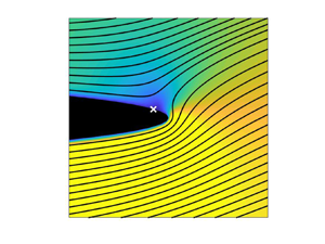
Figure 5. Midplane contour plot of the fluid speed near the trailing edge for (a)  $\varLambda =0.000375$ and (b) $\varLambda =1$ (for both cases $\epsilon =0.005$ and $\delta =0.05$) for an angle of attack of 10 $^\circ$. Streamlines of the velocity field are shown in black. In (a) the location of the RSP for a two-dimensional unbounded potential flow is shown with a white ( $\times$).

Figure 6. The variation of the location of the RSP with increasing (a)  $\epsilon$ (for constant a and $\varLambda$ small enough that the RSP will not move if $\varLambda$ is reduced further) and (b) $\varLambda$, for $\alpha =10^\circ$ for $\delta =0.05$. The dashed grey lines are the potential-flow prediction while the black dashed lines indicate the two-dimensional Stokes-flow prediction (Shintani et al. Reference Shintani, Umemura and Takano1983).
Secondly, the geometry was fixed to have  $\epsilon =0.005$ with $\delta =0.05$ and $\alpha =10^\circ$ and $\varLambda$ was varied in the range $\varLambda \ll \epsilon$ to $\varLambda >1$; the results of which can be seen in figure 6(b). As $\varLambda$ is increased the RSP is at a constant location (note: not at the same location as that for an equivalent ellipse in a two-dimensional unbounded potential flow) until $\varLambda ={O}(\epsilon )$, after which the RSP starts to move towards the trailing edge. This is consistent with the case of the circular cylinder, where the effect of inertia in the boundary layer first occurs when $\varLambda ={O}(\epsilon )$. For $\varLambda >0.5$ the RSP is essentially at the trailing edge, resulting in an attached shear layer, which can be seen in figure 6(b) for $\varLambda =1$.
5.2. Attached shear layer analysis
To investigate the attached shear layer, the geometry is kept fixed with  $\delta =0.05$ and $\epsilon =0.005$ with an angle of attack of $\alpha =10^\circ$. In this analysis, we are interested in the flow when the RSP is at the trailing edge, as can be seen in figure 5(b) (i.e. for $\varLambda >0.5$). The variation of the shear layer (with distance from the trailing edge) can be extracted from the velocity field (for small angles of attack it is possible to only focus on vertical profiles of the horizontal velocity Wood Reference Wood1971) and these are shown in figure 7(a) at various locations in the wake for $\varLambda =0.5,1$ and $1.5$. For higher $\varLambda$, there was a decreased initial shear layer strength at the trailing edge and the rate of decay was less (than for lower $\varLambda$). Following Wood (Reference Wood1971), a curve with the form of (2.37) was fitted to the numerical data (i.e. the dashed lines in figure 7a). As (2.37) has two components, namely, the initial shear layer strength and the exponentially decaying term (which is a function of $\varLambda$), a question arises as to whether to fit the equation to the first or second component. As the initial shear layer strength will be largely determined by the boundary condition on the ellipse, which is different between the numerical simulation and the depth-averaged potential-flow model, it is appropriate that the equation is fitted to the data in the wake (i.e. for $s>0.1$, where $s$ is the non-dimensional distance from the trailing edge). As can be seen from figure 7(a), the rates of decay of the numerical simulations and the model give close agreement. By backward extrapolation, an initial shear layer strength ( $\gamma _0$) can be obtained and using (2.38) an estimation of the bound circulation on the ellipse can be made. This circulation is plotted against $N$ in figure 7(b), together with the analytical prediction from Wood (Reference Wood1971), with close agreement being found.

Figure 7. (a) The variation of the shear layer with non-dimensional distance from the trailing edge of the ellipse for  $\alpha =10^\circ$, where $\varLambda =0.5$ ( $\square$), $1$ (
$1$ ( $*$) and $1.5$ ( $\bigcirc $). The dashed lines are the depth-averaged potential-flow prediction (2.37) matched to the far-field data. (b) The variation of non-dimensional bound circulation per unit radian with $N=15/(4\varLambda )$, where the dashed line is the prediction (2.36) and the estimations (from numerical simulations) are based on the fitted curves in (a).
6. Forces
To investigate the forces on an ellipse in a Hele-Shaw cell, the aspect ratio is fixed to  $\delta =0.05$ and then the effect of varying $\epsilon$ and $\varLambda$ is investigated. As the surface pressure is key to predicting the forces on the ellipse, this will be considered first.
In this work a Joukowski transformation was used to obtain the pressure field around the ellipse, which is only possible under the assumption that the Laplacian of the pressure was zero. For  $\epsilon =0.005$ and $\delta =0.05$, figure 8 shows that there is excellent agreement for $\varLambda \ll 1$ for both angles of attack, $\alpha = 0^\circ$ and 45 $^\circ$. As $\varLambda$ is increased the difference between the linear prediction and the numerical simulations is more pronounced for the case of $\alpha =45^\circ$. The integrated effect of this is discussed below.

Figure 8. Surface pressure profiles for the ellipse at an angle of attack of (a–c) 0 $^\circ$ and (d–f) 45 $^\circ$ for $\varLambda = ({a},{d})$ $0.00375$, (b,e) $0.375$ and (c, f) $1$ with $\epsilon =0.005$ and $\delta =0.05$. The dashed lines are the linear prediction (2.24) for the circular cylinder transformed onto the ellipse using (2.25).
For the first case, the angle of attack was fixed to  $\alpha =10^\circ$ and $\epsilon$ was varied. Note that, for every $\epsilon$ considered, $\varLambda$ was lowered until the RSP was at a constant location (see figure 6b). In figure 9(a,b) the variation of the drag and lift coefficients are shown, together with the pressure drag prediction from (2.26) and (2.27), respectively. The prediction for the drag coefficient is good for small $\epsilon$, with less agreement for $\epsilon ={O}(10^{-1})$. This is because, as $\epsilon$ is increased, the contribution of the pressure drag to the total drag decreases, as seen in figure 9(c). The prediction for the lift coefficient is better for a wider range of $\epsilon$ as the net effect of the shear stress over the upper and lower side is small, resulting in the lift coefficient being mainly determined by the pressure.


For the second case the ellipse was fixed to have  $\epsilon =0.005$ and $\delta =0.05$ and $\varLambda$ was increased. Figure 10(a,b) shows the drag and lift coefficients of the ellipse where the linear prediction is very good up to $\varLambda ={O}(1)$, after which the predictions and the calculations start to diverge. This divergence occurs for lower values of $\varLambda$, for higher angles of attack, which is to be anticipated from the surface pressure profiles seen in figure 8. One possibility of including nonlinear effects when the RSP is at the trailing edge is by using the modified Kutta–Joukowski theorem (2.35). Figure 10(c) shows that the bound circulation term provides a correction to the linear lift coefficient for the case of an angle of attack of 10 $^\circ$ when $\varLambda ={O}(1)$. However, there are significant inertial effects at these higher $\varLambda$ which are not captured with this analysis, leading to the divergence seen in the figures.

Figure 10. Variation of the (a) drag coefficient and (b) lift coefficient with  $\varLambda$ for angles of attack of 0 $^\circ$ ( $\square$), 10 $^\circ$ ( $\lozenge$), 20 $^\circ$ ( $\bigcirc$), 45 $^\circ$ ( $\times$) and 90 $^\circ$ (*) for $\delta =0.05$ and $\epsilon =0.005$. The linear predictions for the pressure induced drag (2.26) and lift (2.27) coefficients are given by the dashed lines. In (c) the prediction (2.35) is shown as ( $\blacklozenge$), which includes the correction due to the bound circulation associated with the attached shear layer.
7. Conclusions
In this work we have used analytical and asymptotic methods and numerical simulations to investigate the flow and force on ellipses in a Hele-Shaw cell. The vertices of the thin ellipses studied here exhibit a Stokes region which makes it not as analytically tractable as a circular cylinder in a Hele-Shaw cell. However, asymptotic predictions were compared with numerical simulations over the flatter part of the ellipse, with close agreement being found. A Joukowski transformation can be used to transform the pressure field of a circular cylinder onto an ellipse, from which the drag and lift coefficients could be derived. This was found to be only appropriate for small  $\epsilon$ where the drag coefficient is dominated by the pressure component. The lift coefficient is less sensitive to this as the net shear force (of the lift coefficient) is small. For $\varLambda ={O}(1)$ (on a point of detail, we mention here that the global Reynolds number $U_c a / \nu$ has to be large for the present inertial effects to come into play), the attached shear layer was analysed and by using a modified Bernoulli equation, together with the Kutta–Joukowski theorem, a correction to the linear prediction was made, which was applicable to low angles of attack.
Flows in Hele-Shaw cells are often used as an analogy to flows in porous media which assumes that the gap thickness and inertia are very small. In this work we have investigated the effect of when these assumptions are not necessarily valid and the limitations of using the developed methods. One possibility of extending this work could be to investigate aerofoils by using a Kármán–Trefftz transformation or other conformal mappings. This might be particularly useful with the recent investigations into deformable Hele-Shaw cells (Box et al. Reference Box, Peng, Pihler-Puzovic and Juel2020).
The flow in the choriocapillaris, a microvascular bed located in the back of the eye, consists of a multipolar Hele-Shaw flow with arteries and veins inserting into the choriocapillaris at approximately right angles. Within the plane of the choriocapillaris blood navigates a varying solid void fraction determined by intervascular spaces called septae. A standard model for the choriocapillaris is a set of sources (arteries) and sinks (veins) connected to one of two parallel sheets, with septae modelled as cylinders spanning the height of the flow domain (Zouache, Eames & Luthert Reference Zouache, Eames and Luthert2015; Zouache et al. Reference Zouache, Eames, Klettner and Luthert2019). Since the depth-averaged expressions (2.30) and (2.31) are general, they may be used to analyse multipolar flows by adding the elemental contributions of sources, sinks and doublets for cylinders to the velocity potential. Future investigations will include proving the validity of these expressions for different geometric and flow parameters.
Acknowledgements
The authors acknowledge the use of the UCL's Myriad High Performance Computing Facility (Myriad@UCL) and Kathleen High Performance Computing Facility (Kathleen@UCL), and associated support services, in the completion of this work.
Declaration of interests
The authors report no conflict of interest.


 Open access