


1. Introduction
Cavitation, the process of bubble formation and collapse, is a key physics problem because of its applications in nature, mechanics, biomedical, and many other fields (Cole & Weller Reference Cole and Weller1948; Lohse, Schmitz & Versluis Reference Lohse, Schmitz and Versluis2001; Ohl et al. Reference Ohl, Arora, Dijkink, Janve and Lohse2006a,Reference Ohl, Arora, Ikink, De Jong, Versluis, Delius and Lohseb; Maxwell et al. Reference Maxwell, Cain, Hall, Fowlkes and Xu2013; Fuster Reference Fuster2019). In recent studies, Hou et al. (Reference Hou, Wang, Yan, Wang and An2021) showed that cavitation bubbles can enhance the efficiency of solar absorption refrigeration systems, and Bhat & Gogate (Reference Bhat and Gogate2021) and Prado et al. (Reference Prado, Antunes, Rocha, Sánchez-Muñoz, Barbosa, Terán- Hilares, Cruz-Santos, Arruda, da Silva and Santos2022) reviewed the effect of cavitation in wastewater and biomass treatment. Lyons et al. (Reference Lyons, Haney, Fee, Wech and Waythomas2019) compared the low-frequency sound signals from volcanic eruptions to that of bubble collapse, and suspect that bubbles of the order of 100 m are created by the interaction of magma with water. Bubbles can generally appear from the nuclei sitting at walls (Crum Reference Crum1979; Atchley & Prosperetti Reference Atchley and Prosperetti1989; Borkent et al. Reference Borkent, Gekle, Prosperetti and Lohse2009), making the interaction with the wall an essential aspect of bubble collapse dynamics. The wall modifies the symmetry of the pressure field near the bubble that causes unequal interface acceleration and thus high-speed liquid jets leading to complex cavitation phenomena (Brenner, Hilgenfeldt & Lohse Reference Brenner, Hilgenfeldt and Lohse2002; Popinet & Zaleski Reference Popinet and Zaleski2002; Supponen Reference Supponen2017). These jets are important in understanding the destructive potential of the cavitation bubbles for several biomedical applications such as the disruption of biological membranes in high-intensity focused ultrasound (HIFU), lithotripsy, histotripsy and sonoporation techniques (Prentice et al. Reference Prentice, Cuschieri, Dholakia, Prausnitz and Campbell2005; Ohl et al. Reference Ohl, Arora, Ikink, De Jong, Versluis, Delius and Lohse2006b; Maxwell et al. Reference Maxwell, Wang, Cain, Fowlkes, Sapozhnikov, Bailey and Xu2011; Pishchalnikov et al. Reference Pishchalnikov, Behnke-Parks, Schmidmayer, Maeda, Colonius, Kenny and Laser2019). Other applications concerning erosion, surface cleaning, noise emission and manufacturing processes (e.g. shot peening) are also closely linked to the phenomenon of jetting (Krefting, Mettin & Lauterborn Reference Krefting, Mettin and Lauterborn2004; Blake, Leppinen & Wang Reference Blake, Leppinen and Wang2015). The bottleneck in development and comprehension of these techniques as well as naturally occurring phenomena remains the limited understanding of the interaction between a cavitation bubble and its surrounding medium.
It is well known that the jets formed during the collapse of bubbles in the presence of a nearby wall are directed towards the wall and that the characteristics of these jets can be described well using the scaling laws given by Popinet & Zaleski (Reference Popinet and Zaleski2002) and Supponen (Reference Supponen2017). However, investigations on the collapse of a bubble initially attached to a wall are reported less often. Naudé & Ellis (Reference Naudé and Ellis1961) discuss the collapse of a bubble initially in contact with a wall by writing the higher-order perturbation solutions to the potential flow model. They also show the collapse dynamics of such bubbles experimentally by producing bubbles with an electric spark in the liquid close to the wall. Hupfeld et al. (Reference Hupfeld, Laurens, Merabia, Barcikowski, Gökce and Amans2020) present experimental results for laser-induced bubbles using ultra-high-speed photography in the high-capillary-number regimes. They study both expansion and collapse phases in several liquids to understand the effect of viscosity on growth, collapse and bubble shapes, including liquid microlayer and contact line evolution. Both Naudé & Ellis (Reference Naudé and Ellis1961) and Hupfeld et al. (Reference Hupfeld, Laurens, Merabia, Barcikowski, Gökce and Amans2020) show that during the collapse the jet is directed towards the solid, whereas Li et al. (Reference Li, Zhang, Wang and Han2018) show that the jet can be directed in the opposite direction when a collapsing bubble is in contact with a spherical solid particle. A similar problem is studied numerically by Lechner et al. (Reference Lechner, Lauterborn, Koch and Mettin2020), who also include the effect of bubble expansion and the liquid microlayer that results in a different nature of bubble collapse and jetting. This problem has also been discussed briefly in numerical studies of Lauer et al. (Reference Lauer, Hu, Hickel and Adams2012) and Koukouvinis et al. (Reference Koukouvinis, Gavaises, Georgoulas and Marengo2016), who observe the change in jetting behaviour as a function of bubble shape, but they do not show jets opposite to the wall. Reuter et al. (Reference Reuter, Gonzalez-Avila, Mettin and Ohl2017) speculate on the appearance of a jet parallel to the wall during the secondary collapse, and consequently the generation of a vortex ring, although no direct experimental observation is reported.
The initiation and consequences of this change of behaviour has not been understood, and a hydrodynamic description of it is not available. In this paper, we bridge this gap and describe the factors controlling the jetting direction using comprehensive theoretical numerical and experimental evidence. We clarify that the change in the jetting direction is an implication of the singularity in the pressure gradient obtained from the potential flow model. This singularity appears only when the effective contact angle at the instant before the collapse is larger than  $90^{\circ }$. We show that at short instants after beginning of collapse phase, and for sufficiently large Reynolds and Weber numbers, the potential flow solution represents accurately the results of direct numerical simulations (DNS). Despite the fact that viscosity instantaneously regularises the solution near the singularity and predicts finite velocities, the effect of the singularity is still present outside the boundary layer, and it explains the changes in the nature of the jet generated. In addition, we show that there is a direct link between the bubble response at short times and the formation of a vortex ring that eventually leads to surprising long-range interaction effects between the bubble and a free surface (see supplementary movie 3 available at https://doi.org/10.1017/jfm.2022.705) that have not been reported before. These results provide a significant advance in the characterisation of the interaction mechanisms between a bubble and its surrounding medium, and may provide reasoning behind unexplained delayed effects in underwater explosions observed by Kedrinskii (Reference Kedrinskii1978), and tsunami generation by underwater volcano eruptions (Paris Reference Paris2015).
2. Problem set-up
We focus on the classical three-dimensional Rayleigh collapse problem for a bubble that has a spherical cap shape (figure 1). This choice is motivated by the fact that for a spherical cap, the bubble geometry is defined by only two parameters, the bubble radius and the contact angle, which simplifies the discussion of the results compared to more complex shapes (e.g. ellipsoids) that could be a focus of future investigations. We restrict ourselves to an axisymmetric configuration where the initial bubble pressure  $p_{g,0}$ is uniform inside the bubble, and the liquid, initially at rest, is at a higher pressure far from the bubble $p_\infty > p_{g,0}$. This problem represents the solution of a bubble in equilibrium state subjected to impulsive action caused by a sudden increase in far-field pressure, and is also a good approximation for the dynamic response of a low-pressure bubble after the expansion stage when it reaches its maximum radius and the liquid velocity approaches zero.

Figure 1. Problem set-up and the different coordinate systems used in this paper, i.e.  $(r_w,\theta _w)$ and $(r_s,\theta _s)$.
The dynamics of this system is governed by the mass, momentum and energy conservation laws, which for the  $i$th component in a multi-component set-up are
 $$\begin{gather} \frac{\partial \rho_i}{\partial t} + \boldsymbol{\nabla} \boldsymbol{\cdot} (\rho_i {\boldsymbol u}) = 0, \end{gather}$$
 $$\begin{gather}\frac{\partial \rho_i {\boldsymbol u}}{\partial t} + \boldsymbol{\nabla} \boldsymbol{\cdot} (\rho_i {\boldsymbol u}{\boldsymbol u}) ={-}\boldsymbol{\nabla} p_i + \boldsymbol{\nabla} \boldsymbol{\cdot} {\boldsymbol{\tau}}_i, \end{gather}$$
 $$\begin{gather}\frac{\partial (\rho_i E_i)}{\partial t} + \boldsymbol{\nabla} \boldsymbol{\cdot} (\rho_i E_i \boldsymbol{u}) ={-} \boldsymbol{\nabla} \boldsymbol{\cdot} ({\boldsymbol u}p_i) + \boldsymbol{\nabla} \boldsymbol{\cdot} ({\boldsymbol{\tau}}_i {\boldsymbol u}). \end{gather}$$
As usual,  $\boldsymbol {u}$ represents the velocity vector field, $\rho _i$ is density, $p_i$ is the pressure field, and ${\boldsymbol{\tau}}_i = \mu _i (\boldsymbol {\nabla } {\boldsymbol u} + (\boldsymbol {\nabla } {\boldsymbol u})^{\rm T})$ is the viscous stress tensor for each component. The total energy $\rho _i E_i = \rho _i e_i + \tfrac {1}{2} \rho _i {\boldsymbol u} \boldsymbol {\cdot } {\boldsymbol u}$, is the sum of internal energy per unit volume $\rho _i e_i$, and kinetic energy $\tfrac {1}{2} \rho _i {\boldsymbol u} \boldsymbol {\cdot } {\boldsymbol u}$ per unit volume. Finally, the equation of state is written as $\rho _i e_i = ({p_i + \varGamma _i \varPi _i})/({\varGamma _i - 1})$, where $\varGamma$ and $\varPi$ are adopted from Johnsen & Colonius (Reference Johnsen and Colonius2006) in such a way that the liquid is slightly compressible and the bubble contents obey an ideal gas equation of state. The system of equations is closed by adding an advection equation for the interface position, which is represented by the volume of fluid method (Tryggvason, Scardovelli & Zaleski Reference Tryggvason, Scardovelli and Zaleski2011). After the advection, the interface is reconstructed using a piecewise linear interface construction. The surface tension appears implicitly while averaging (2.1a) in the mixed cells, and it is added as the continuum surface force using the method of Brackbill, Kothe & Zemach (Reference Brackbill, Kothe and Zemach1992), also reviewed recently by Popinet (Reference Popinet2018). All the intricate details of the method are given in Fuster & Popinet (Reference Fuster and Popinet2018)
In the DNS, a non-slip boundary condition is imposed on the velocity field at the wall, while a standard free-flow condition is applied in all the other boundaries. Note that although a non-slip boundary condition imposes zero velocity at the boundary, the velocity at which the interface is advected in the cell adjacent to the wall is different from zero. This acts effectively as an implicit slip length for the contact line motion given as  $\lambda = \Delta x_{min}/2$, where $\Delta x_{min}$ is the smallest grid size. The influence of this parameter will be discussed in Appendix A. The static contact angle model proposed by Afkhami & Bussmann (Reference Afkhami and Bussmann2008) is used to implement a contact angle boundary condition that, although not very accurate for prediction of the contact line motion, is a convenient tool that gives fair insight into the growth of the boundary layer and range of influence of viscosity. More sophisticated models for contact line motion could be used, but a significant change in the conclusions of this work is not expected.
The initial conditions are defined by imposing the fluid to be initially at rest ( $\boldsymbol {u}=0$). In this case, the divergence of the momentum equation gives a Laplace equation for the initial liquid pressure, assuming that the liquid is an incompressible substance:
 \begin{equation} \Delta p_l = 0. \end{equation}
This equation is solved readily if we assume that the gas pressure is initially uniform such that the boundary conditions for pressure (as shown in figure 1) are as follows. At the interface, the liquid pressure is
 \begin{equation} p_{0,L}=p_{g,0} - \frac{2\sigma}{R_c}, \end{equation}
where  $\sigma$ is the surface tension coefficient, and $R_c$ is the radius of curvature. At the far-away boundaries, the pressure is $p_\infty$, and at the wall, the normal pressure gradient is null due to the impermeability condition. The initial condition for total energy is then calculated from the equation of state using the initial pressure field.
Finally, we introduce relevant dimensionless quantities using the radius of curvature as characteristic length, the liquid density, and the characteristic velocity  $U_c= ({p_\infty }/{\rho _l})^{1/2}$ obtained by assuming that at the instant of maximum radius, the liquid pressure along the surface is negligible compared to the far-field pressure. A simple dimensional analysis shows that the solution of the problem depends on the density and viscosity ratios, the Reynolds number ${Re} = {\rho _l U_c R_c}/{\mu _l}$, the Weber number ${We} = {\rho _l U_c^2 R_c}/{\sigma }$, and the contact angle $\alpha$. The characteristic velocity is constant and equal to $10\,{\rm m}\,{\rm s}^{-1}$ for the low-pressure bubbles collapsing in water under the action of the atmospheric pressure; therefore both the Reynolds and Weber numbers are determined by only the radius of curvature of the bubble. In the particular experiments considered in this study, the radius of curvature remains of the order of 1 cm, obtaining characteristic values of the Weber and Reynolds numbers of the order of ${We} \sim {O}(10^4)$ and ${Re} \sim {O}(10^5)$. The influence of finite values of the Reynolds number is discussed briefly using DNS.
3. Short-time dynamics
At short times, we can simplify the system of equations if we consider the liquid as an incompressible substance and the interface as a free surface, i.e. we neglect inertial and viscous effects inside the bubble. This assumption is reasonable given that  $\mu _g/\mu _l \ll 1$ and $\rho _g/\rho _l \ll 1$. (In experiments, the density ratio is of the order of $10^{-5}$ when the bubble pressure equals the vapour pressure.) The velocity at short times remains a small quantity, thus we can neglect the convective terms as compared to temporal derivatives of velocity and spatial pressure gradients (Batchelor Reference Batchelor2000). This hypothesis remains true when time scales under consideration are smaller than the advection time scales, i.e. ${t_s U_c}/{R_c}\ll 1$. Under these assumptions, the solution for the velocity is obtained from the integration of the linearised momentum equation as
 \begin{equation} {\boldsymbol u}(t_s) ={-} \frac{1}{\rho} \int_0^{t_s} \boldsymbol{\nabla} p + \frac{1}{\rho} \int_0^{t_s} \boldsymbol{\nabla} \boldsymbol{\cdot} {\boldsymbol \tau}. \end{equation}
It is classical for this linear system to decompose the velocity field into a potential part  ${\boldsymbol u}_\phi$ and a viscous correction ${\boldsymbol u}_\nu$, i.e. ${\boldsymbol u} = {\boldsymbol u}_{\phi } + {\boldsymbol u}_{\nu }$. The potential flow theory gives ${\boldsymbol u}_\phi$, whereas the viscous correction requires complex analysis (Saffman Reference Saffman1995; Batchelor Reference Batchelor2000; Pope Reference Pope2000). For short times and large enough Reynolds numbers, the viscous contributions to velocity are relevant only in the small region of thickness $\delta \sim {O}(\sqrt {\nu t})$ near the solid boundary. Thus in such a situation, we expect the solution to be governed by the potential part, and the viscous part is only a correction in a thin region close to the wall. We discuss these aspects next.
3.1. Potential flow solution
The potential flow solution is obtained by solving the inviscid part of the linearised momentum equation
 \begin{equation} \frac{\partial {\boldsymbol u}_{\phi}}{\partial t} ={-}\frac{1}{\rho}\,\boldsymbol{\nabla} p. \end{equation}
The magnitude of the pressure gradient field (or acceleration field) at short infinitesimal times governs the dynamics of bubble collapse at a finite time. To obtain the acceleration, we introduce the dimensionless pressure  $\tilde {p}=({p-p_{0,L}})/({p_\infty - p_{0,L}})$. Note that in the linear problem, the interface does not move, therefore surface tension effects at short times only introduce a correction on the scaling prefactor $(p_\infty -p_{0,L})$ upon which the solution depends. The divergence of (3.2) leads to a Laplace equation ( $\Delta \tilde{p} = 0$) that can be solved with appropriate boundary conditions for $\tilde {p}$. In particular, we impose $\tilde {p}=1$ far away from the bubble, $\tilde {p}=0$ at the bubble interface, and ${{\rm d}\tilde {p}}/{{\rm d}n} = 0$ at the solid boundary. The solution of this equation depends only on the geometry of the bubble, which is fully described as a function of the contact angle $\alpha$. This simplified representation of the fluid fields at short times is referred as the ‘free surface model’ in this paper.
In figure 2(a), we start presenting the isocontours of the magnitude of the non-dimensional acceleration ( $|\boldsymbol {\nabla } \tilde {p}|$) field obtained for a spherical cap bubble with contact angle $\alpha = {3}{\rm \pi} /{4}$, while figure 2(b) shows the variation of the same along the wall in the liquid phase with respect to the distance from the contact line obtained from the free surface model. The isocontours in the left half are obtained numerically from the free surface model, while those in the right half are obtained from the DNS of the Navier–Stokes equations (using the set-up shown in figure 4a), accounting for the presence of a gas with non-zero density ( $\rho _l/\rho _g = 10^{-3}$) and a finite value of viscosity ( $\mu _l/\mu _g = 10^{-2}$) at ${t U_c}/{R_c} = 2.07 \times 10^{-6}$. Good agreement between the two models supports the argument that (2.2) is a good representation of the fluid dynamics at very short times. We distinguish clearly two separate regions: the far field where the pressure gradient contours are hemispherical caps centred at the axis of symmetry, and the near field where the contours for pressure gradient are intricate and diverge on approaching the triple contact point. Next, we characterise each of these regions.

Figure 2. (a) Isocontours of the magnitude of acceleration for a bubble with  $\alpha = 3{\rm \pi} /4$. The isocontours in the left half are obtained from the free surface model, and those in the right half are obtained from DNS. (b) Non-dimensional acceleration magnitude along the wall obtained for a bubble with $\alpha =3{\rm \pi} /4$ using the free surface model.
3.1.1. Near field
The numerical solution of the interface acceleration at the initial time is shown in figure 3(a), where we use the angle with respect to the solid wall  $\theta _w$ to parametrise the interface position. The origin $\theta _w = 0$ corresponds to the point of contact between the interface and the solid wall, and $\theta _w={\rm \pi} /2$ is the intersection of the interface with the axis of symmetry. Figure 3(a) depicts the local non-dimensional acceleration magnitude at bubble interface $\vert {\boldsymbol a} \vert /a_0$ for four representative cases with $\alpha ={\rm \pi} /3, {\rm \pi}/2, 2{\rm \pi} /3,3{\rm \pi} /4$. The value of the reference acceleration is chosen as $a_0 = ({p_\infty - p_{0,L}})/{\rho R_c}$, which is the acceleration magnitude for a spherical bubble with radius $R_c$ and a known pressure difference. As expected, in the case $\alpha = {\rm \pi}/2$, the numerical solution recovers the Rayleigh–Plesset solution, and the non-dimensional acceleration is uniform and equal to 1 all over the interface. When $\alpha < {\rm \pi}/2$, the interface acceleration (thus velocity) tends to zero at the contact point, and therefore it ceases to move even in the potential flow problem with a slip wall. For $\alpha > {\rm \pi}/2$, the appearance of the singularity is evident as the acceleration diverges as we approach the $\theta _w\to 0$ limit. To interpret this result, one must keep in mind that the general solution of the Laplace equation in spherical coordinates can be obtained by separation of variables that leads to an infinite series. This series sometimes diverges at the edge where Dirichlet and Neumann boundary conditions meet due to the appearance of a singularity (Dauge Reference Dauge2006). This singularity was reviewed extensively in the past (Landau & Lifshitz Reference Landau and Lifshitz1959; Blum & Dobrowolski Reference Blum and Dobrowolski1982; Steger Reference Steger1990; Deegan et al. Reference Deegan, Bakajin, Dupont, Huber, Nagel and Witten1997; Li & Lu Reference Li and Lu2000), but studies where this singularity appears in bubble dynamics problems are rare. The asymptotic solutions close to the point where homogeneous Dirichlet and Neumann boundary conditions meet can be expressed alternatively by using the general solution of the Laplace equation (Li & Lu Reference Li and Lu2000; Dauge Reference Dauge2006; Yosibash et al. Reference Yosibash, Shannon, Dauge and Costabel2011), and take the form
 \begin{equation} \tilde{p}_s= \sum_k^\infty C_k \tilde{r}_s^{b_k} \cos\left(b_k \theta_s \right), \end{equation}
where  $\tilde {r}_s=r_s/R_c$ is the non-dimensional distance from the contact line, and $b_k=({{\rm \pi} }/{\alpha }) (k+1/2)$. Taking the derivative with respect to the normal of the interface, we readily find the interface acceleration magnitude near the contact line as
 \begin{equation} \vert {\boldsymbol a}_I \vert = \frac{1}{\rho} \left| \frac{\partial p}{\partial n} \right| \approx a_0 C_0 b_0 \tilde{r}_s^{b_0 - 1}. \end{equation}
This expression exhibits a singularity at the contact point ( $r_s \to 0$) when $b_0 = {{\rm \pi} }/{2\alpha } < 1$ (or $\alpha > {\rm \pi}/2$), implying that the acceleration at the triple contact point is infinite. In these conditions, the first term in the expansion is the leading-order term that eventually dominates the solution in the region $r_s \le R_c$. This can also be seen clearly in figure 2(b), where the fitting curve shown with a solid line is obtained using the first term of the series solution (i.e. parameters $C_0$ and $b_0$ in (3.4)). We repeat the fitting procedure for various $\alpha$ to verify that the numerical values of $b_0$ match well with theoretical predictions, and find $C_0$ that is a constant of order 1 that increases slightly with $\alpha$ (figure 3b).

Figure 3. (a) Non-dimensional acceleration magnitude  ${\vert {\boldsymbol a}_I\vert }/a_0$ along the interface parametrised using the angle $\theta _w$ (measured in the counter-clockwise direction from the point of contact of wall and the axis of symmetry) for $\alpha = {{\rm \pi} }/{3},{{\rm \pi} }/{2},{2}{\rm \pi} /{3},{3}{\rm \pi} /{4}$. Dots represent the numerical solution from the free surface model, and the thick lines are predictions using (3.4) evaluated at the interface. (b) Exponent $b_0$ and coefficient $C_0$ obtained from fitting the pressure gradient obtained from the free surface model along the wall for different $\alpha$. (c) Non-dimensional averaged interface acceleration magnitude as a function of the contact angle using different methods: analytical expression given by (3.6) (blue line), the solution from the free surface model (yellow line), the DNS solution of the Euler equations (black crosses), and the DNS solution of the Navier–Stokes (NS) solver for ${Re}=100$ (red crosses).
Focusing on the characterisation of the regimes where the singularity appears, figure 3(a) shows clearly that the numerical solution (dots) is well described by (3.4) evaluated at the interface (solid lines), showing excellent agreement close to the contact point, i.e. small values of  $\theta _w$. Near the axis of symmetry (e.g. $\theta _w\to {\rm \pi}/2$ and $\tilde {r}_s \approx 1$), the errors are visible and the first term in the series does not suffice to describe accurately the acceleration field.
3.1.2. Far field solution
The far field flow created by the bubble corresponds to a punctual sink sitting at the intersection between the wall and the axis of symmetry. The integration of the momentum equation in the radial coordinate provides the magnitude of the pressure gradient generated by a punctual sink at an arbitrary distance from the sink as
 \begin{equation} \left| \frac{{\rm d}\tilde{p}_{{far}}}{{\rm d}\tilde{r}_w} \right| = \frac{\vert \bar{\boldsymbol a}_I \vert}{a_0}\,\frac{1 + \cos(\alpha)}{\tilde{r}^2_w}, \end{equation}
where  $\vert \bar {\boldsymbol a}_I \vert$ is the magnitude of averaged acceleration along the interface, which determines the strength of the punctual sink. Figure 2(b) shows clearly that this equation captures well the decay of the pressure gradient at distance $\tilde {r}_w$ far from the interface. Because the first term of the series, i.e. (3.4), predicts the interface acceleration reasonably well, we obtain an estimation of the averaged acceleration magnitude for bubbles with $\alpha > {\rm \pi}/2$ as
 \begin{equation} \vert \bar{\boldsymbol a}_I \vert = \left| \frac{1}{S_b} \int \frac{-1}{\rho_l}\,\frac{\partial p}{\partial n}\,{\rm d}S_b \right| = a_0 C_0 b_0\,G(\alpha), \end{equation}
where  $S_b$ stands for the bubble interface surface, and $G(\alpha )$ is a geometrical factor that can be computed numerically, assuming that the first term in the series is indeed the leading-order term along the entire bubble interface. Figure 3(c) shows the averaged non-dimensional interface acceleration magnitude obtained using this model, which compares well with the numerical results of the free surface model and the solution of both the viscous and inviscid Navier–Stokes equations. The results of the simplified model are obtained using the value of $C_0$ computed numerically and reported in figure 3(b). For $\alpha > {\rm \pi}/2$, $\vert \bar {\boldsymbol a} \vert$ increases with $\alpha$. The three proposed models agree well for the angles tested, implying that the free surface model as well as the simplified expression given in (3.6) capture well the averaged bubble response at short times for sufficiently large Reynolds numbers.
3.2. Viscous correction
The potential flow solution is formally exact only at the initial time  $t = 0$ when the interface is at rest. As soon as the interface is set in motion, a thin boundary layer develops immediately, regularising the flow close to the contact point. We use the results from the DNS of the Navier–Stokes equations at short times to investigate the influence of viscosity on the dynamic response of the bubbles.
We solve for the full set of (2.1a) where, for the sake of simplicity, we neglect surface tension effects. The equations are solved using the All-Mach implementation (Popinet Reference Popinet2015; Fuster & Popinet Reference Fuster and Popinet2018), where the one-fluid approach is used to solve the modelling equations. This solver has been used successfully already to investigate some aspects of the interaction of an oscillating bubble and a rigid tube by Fan, Li & Fuster (Reference Fan, Li and Fuster2020), and interactions of collapsing bubbles with a free surface by Saade et al. (Reference Saade, Jalaal, Prosperetti and Lohse2021). The set-up for numerical simulations is shown in figure 4(a), where a spherical-cap-shaped bubble is initialised in a square domain of size 100 times the initial radius of curvature of this bubble. We use such large domains so that the pressure waves reflected from the boundaries do not affect the solution; moreover, the grid is coarsened away from the bubble to diffuse these waves. The simulations are axisymmetric about the left-hand boundary, and the bubble is initially in contact with the bottom boundary where a non-slip boundary condition is applied. The far-away boundaries are given constant far-field pressure conditions and a homogeneous Neumann condition for velocity. The grid is refined progressively near the interface to a minimum grid size  $\Delta x_{min}/R_c = 0.00038$. The maximum time step in the simulation is governed by an acoustic Courant–Friedrichs–Lewy restriction, which in our case is 0.4. The initial pressure field inside the domain is given by (2.2), the velocity field is given as zero, and the total energy is given by the equation of state.

Figure 4. (a) The numerical setup for DNS. (b) Results from the DNS for  $\alpha = 2 {\rm \pi}/3$ and ${Re} = 100$: time-averaged interface acceleration in the direction parallel to the wall, $a_{r,I} = u_{r,I}/t$, as a function of the distance from the wall at five different times (in colour where $t U_c/R_{c,0}\in [7.27 \times 10^{-5},3.6 \times 10^{-4}]$). For reference, we include the potential flow solution given by (3.4) evaluated at the interface (solid black line). The inset represents a zoom in to the viscous boundary layer generated close to the wall.
In figure 4(b), we characterise the bubble motion at short non-dimensional time  $t U_c/R_{c}$ by showing the evolution of the time-averaged interface acceleration magnitude parallel to the wall, defined as $a_{r}(t) = u_r(t)/t$, as a function of the normal distance from the wall. The results shown with coloured dots are obtained from DNS for $\alpha = 2{\rm \pi} /3$ and ${Re} = 100$, where the colour scale represents the non-dimensional time varying between $7.27 \times 10^{-5}$ and $3.6\times 10^{-4}$. The inset shows the clear development of a boundary layer very close to the wall; the thickness of this layer is defined by the height for which the velocity is maximum. Outside this region, the free surface potential flow solution (3.4), shown with a solid black line, predicts the interface velocity obtained from DNS relatively well, therefore the potential flow solution is a good approximation of the collapse process outside the viscous boundary layer. Inside the viscous boundary layer, the interface acceleration is sensitive to the slip length imposed (see Appendix A) and also to the movement of the contact line. In this region, the solution of the free surface model at $t=0$ cannot be extrapolated to predict the flow field near the contact line at short times. Remarkably, although the contact line motion is grid-dependent, the average acceleration and the maximum jet velocity are shown to be independent of the slip length imposed (see Appendix A). This fact, together with the slight dependence of the average acceleration on ${Re}$ (figure 3c), confirms that for large enough Reynolds numbers, the bubble dynamic response is governed mainly by the potential flow solution and not by the particular contact line motion model used. In these conditions, the free surface potential flow model at $t=0$ is a useful tool to predict the average dynamics of the interface at short times.
In order to characterise the jet formation process, we extract the maximum interface velocity magnitude from the DNS data, which we name the jet velocity  ${u}_{jet}$. This velocity is fitted using a power-law function of the form (figure 5a)
 \begin{equation} \frac{u_{jet}}{U_c} = A \left( \frac{t U_c}{R_c} \right)^q, \end{equation}
where  $q$ is a coefficient that becomes smaller than 1 when the acceleration is singular at $t=0$. A theoretical estimation of coefficient $q$ accounting for viscous effects can be obtained from the singular solution described in the previous subsection as follows. The jet velocity after a short time $t_s$ can be approximated from the initial acceleration evaluated at the interface at height equal to the thickness of the boundary layer $z=\delta (t_s)$. The $\delta$ is given approximately by the solution of the Stokes problem for the flow near the flat plate that is started impulsively from rest, therefore we can impose that $\delta (t_s) \approx C_\delta \sqrt {\nu t_s}$, where $C_\delta$ is a constant of order unity. In this case, the jet velocity velocity is estimated as
 \begin{equation} u_{jet} (t_s) = a_{r,I} \left(t=0, z_I=\delta(t_s)\right) t_s, \end{equation}
where we assume that the interface decelerates quickly as soon as it enters inside the viscous boundary layer. Under these assumptions, the coefficient  $q$ is obtained readily as
 \begin{equation} q=\frac{1}{2} + \frac{\rm \pi}{4\alpha}. \end{equation}

As shown in figure 5(b), this model is capable of capturing the evolution of the jet velocity at short times found from DNS simulations accounting for viscous effects when  $\alpha > {\rm \pi}/2$. The exponent $q$ (figure 5b) decreases as $\alpha$ increases because the acceleration gradient in the normal direction increases with $\alpha$, as seen in figure 3(a). Note that the DNS results confirm that $q < 1$ for $\alpha > {\rm \pi}/2$, and therefore the jet acceleration is singular at $t=0$ even in the presence of viscous effects.
Another interesting quantity to describe the overall interface dynamics is the vorticity generated during the collapse. At short times, vorticity is concentrated in a sheet vortex at the wall and at the interface. By assuming a zero stress condition at the interface for  $t = 0$, the only non-zero component of the vorticity can be written as
 \begin{equation} \omega_\phi ={-} 2\,\frac{\partial {u}_r}{\partial \theta}. \end{equation}
It follows from the potential flow solution (figure 3a) that the sign of the acceleration gradient changes depending upon initial contact angle, i.e. if it is greater or less than  ${\rm \pi} /2$, reversing the sign of the vortex sheet generated at the interface. This behaviour is indeed observed from the numerical simulations as shown in figures 6(a,b), where the strength of the vortex sheet is plotted with saturated colour maps. The change in dominant colour represents the opposite sign of vorticity at the interface between the two cases.

Figure 6. The vorticity is shown in colour map and velocity vectors obtained from DNS after a short time ( ${t U_c}/{R_c} = 0.1$) for ${Re} = 100$, for (a) $\alpha = 2 {\rm \pi}/3$, and (b) $\alpha = 5 {\rm \pi}/12$.
4. Long-time dynamics
4.1. High-Reynolds-number regime
Having described the short-time dynamics, in this section we investigate the long-time consequences of this singular response using the experiments and DNS. The results for two representative cases  $\alpha > {\rm \pi}/2$ and $\alpha < {\rm \pi}/2$ shown in figures 7(a,b) are discussed now.

Figure 7. Snapshots of bubble shapes are shown for the two representative cases; the numerical bubble shapes, shown with red curves, are overlaid at same times and scaled to the same length as in the experiments. (a) Case where  $\alpha > {\rm \pi}/2$; snapshots are taken every $0.1$ ms. (b) Case where $\alpha < {\rm \pi}/2$; snapshots are taken every $0.125$ ms.
4.1.1. Dynamics of bubbles with an effective contact angle larger than  ${\rm \pi} /2$

First, we discuss the case where the singularity is present (e.g.  $\alpha > {\rm \pi}/2$). The generation of bubbles with $\alpha > {\rm \pi}/2$ can be investigated using the set-up described briefly in Appendix B, and Bourguille et al. (Reference Bourguille, Bergamasco, Tahan, Fuster and Arrigoni2017) and Tahan et al. (Reference Tahan, Arrigoni, Bidaud, Videau and Thévenet2020). The laser is focused at the bottom of a liquid tank where a water drop is attached. The cavitation in the water drop induces a shock wave in the aluminium plate that leads to the appearance of multiple bubbles in the water tank that interact to form a flat bubble with shape similar to a spherical cap at maximum volume (figure 7a). The snapshots are taken every $0.1$ ms; the interface from the second snapshot is extracted and fitted with an approximate spherical cap which gives $R_c = 7.56\times 10^{-3}$ m and $\alpha = 0.727 {\rm \pi}$.
We reproduce the experimental conditions numerically using the numerical set-up described in § 3.2. The minimum mesh size is  $\Delta x = 60\,\mathrm {\mu }{\rm m}$, the far-field pressure $p_\infty$ is 1 atm, and the pressure inside the bubble is set to the low value 0.1 atm, which is chosen by trial and error to match the numerical collapse time with the collapse time in experiments. We consider both surface tension and viscous effects in the numerical simulations, with ${Re} \approx 75\,600$ and ${We} \approx 10\,500$. The numerically obtained bubble shapes plotted with red contours, and scaled to bubble size in snapshot 2, are subsequently overlaid on the experimental snapshots after the same times. Very good agreement is seen between the numerical and experimental bubble shapes; small differences persist because of the simplification of the bubble shape during the expansion, and the influence of gravity, mass transfer and other effects that are not considered in the numerical simulations.
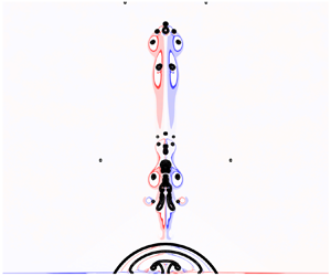
At the beginning of the collapse phase, the highest interface velocity is developed at the edge of the viscous boundary layer (see figure 4b), which leads to the appearance of an annular jet that is generated parallel to the wall, and a mushroom-like shape of the interface contour (see figure 7(a) and supplementary movie 1). These results are consistent with previous numerical works of Lauer et al. (Reference Lauer, Hu, Hickel and Adams2012) and Koukouvinis et al. (Reference Koukouvinis, Gavaises, Georgoulas and Marengo2016). Remarkably, when the collapse is strong enough and the jet reaches the axis of symmetry, a stagnation point appears there, and a secondary upward jet normal to the wall is generated. The re-entrant jet observed for  $\alpha > {\rm \pi}/2$ is not conventional in cavitation and generates vortex ring structures similar to those observed by Reuter et al. (Reference Reuter, Gonzalez-Avila, Mettin and Ohl2017) that are persistent in nature and can travel large distances in comparison to bubble size. The generation of this vortex ring is illustrated numerically in figure 8(a), where the colour maps show the vorticity field. A clear re-entrant annular jet is observed, followed by a mushroom like structure, and the bubble detaches from the wall; consequently a jet in the upwards direction leads eventually to formation of a vortex ring. In the experiments, we visualise this by adding dye in the bottom of the tank (figure 8b) during the collapse of a flat bubble. This vortex ring can travel to a long distance and induce unusual long-range effects like free surface waves and jetting (see supplementary movie 3).

Figure 8. (a) Bubble interface in black curve and the vorticity field in the colour map as obtained from DNS, shown at (consecutively from left to right)  ${t U_c}/{R_c}= 0,0.19,0.3,0.81,1.00,1.45,1.95,4.90$. The annular jet parallel to the wall reaches the axis, resulting in the jet being directed away from the wall, which later generates the vortex ring. The results are plotted for $\alpha = 2{\rm \pi} /3$, ${Re} = \infty$ and ${We} = \infty$. (b) Visualisation of the liquid flow field obtained by adding dye at the bottom of the tank, resulting from collapse of the bubble, shown at every 2.5 ms.
4.1.2. Dynamics of bubbles with an effective contact angle smaller than ${\rm \pi} /2$

The dynamics of bubbles with contact angles smaller than  $90^{\circ }$ (figure 7b) can be obtained using a classical experiment where a laser is focused directly into the liquid very close to the wall. The bubble shape from snapshot 2 in figure 7(b) is approximated with a spherical cap that gives $R_c = 7.63\times 10^{-3}\,{\rm m}$ and $\alpha = 0.389 {\rm \pi}$. The interface contours obtained numerically are shown with the red curves scaled to the size of the bubble in the first snapshot. In this case, the interface acceleration is minimum at the contact line and maximum at the tip of the spherical cap, leading to a conventional high-speed liquid jet directed towards the wall (see figure 7(b) and supplementary movie 2). This jet developed towards the wall impinges into the solid surface, causing cavitation damage. Similar dynamics has been described in several previous studies (Naudé & Ellis Reference Naudé and Ellis1961; Gonzalez-Avila, Denner & Ohl Reference Gonzalez-Avila, Denner and Ohl2021).
4.2. Finite-Reynolds-number effects
Popinet & Zaleski (Reference Popinet and Zaleski2002) showed that for small bubbles collapsing in the vicinity of a rigid wall, the jets can be suppressed due to the viscous effects. In this subsection, we use the DNS to predict quantitatively the range of size for which the observations reported in this paper apply. We take an ideal case of an air bubble with  $p_{b,0} = 0.1$ atm and constant contact angle equal to $120^{\circ }$ collapsing in water at an ambient far-field pressure. In this situation, the characteristic velocity of the process stays constant and equal to $10\,{\rm m}\,{\rm s}^{-1}$, and the initial radius of curvature is then left as the unique parameter controlling the values of the Reynolds and Weber numbers.
In figure 9(a), we show the maximum non-dimensional velocity reached during the collapse as a function of the Reynolds number. For Reynolds numbers above a given critical value,  ${Re} > {Re}_c= 100$, the influence of the Reynolds number on the peak velocities is only marginal. However, when the Reynolds number is below this critical value, the jet velocity drops dramatically further, decaying with decreasing ${Re}$. This sudden change in the peak velocities is controlled by the appearance of jetting, which is not visible for ${Re} \leq 100$ (see figure 9b). For a low-pressure air bubble collapsing in water at atmospheric pressure, these results reveal that the observations reported (reversed re-entrant jet) are applicable for bubbles larger than $R_c > 10\,\mathrm {\mu }{\rm m}$. We must still emphasise that the results reported here are limited to spherical cap bubbles. In reality, other kinds of behaviour can be observed depending on the mechanism by which the bubbles are generated and the bubble shape reached at the instant of maximum expansion. If the bubble shape is not a spherical cap, or the microlayer is not able to drain during the bubble collapse, or the bubble size is comparable to pits, then it can lead to a variety of other collapse and jetting dynamics discussed by Lechner et al. (Reference Lechner, Lauterborn, Koch and Mettin2020), Reuter & Ohl (Reference Reuter and Ohl2021) and Trummler et al. (Reference Trummler, Bryngelson, Schmidmayer, Schmidt, Colonius and Adams2020), respectively.

Figure 9. (a) Peak of the non-dimensional velocity as a function of Reynolds number for an air bubble at  $p_0=0.1$ atm collapsing in water at atmospheric pressure. (b) Interface contours as a function of the Reynolds number at the instant of minimum radius.
5. Conclusions
In this work, we show that impulsive potential flow theory can be used to discuss the influence of bubble shape on the dynamic response of collapsing bubbles for sufficiently large Reynolds and Weber numbers. As an example, we present the results obtained for the collapse of spherical cap bubbles, showing that the effective contact angle at the instant of maximum expansion controls the interface acceleration at the beginning of the collapse phase and the jetting direction observed in DNS and experiments. When  $\alpha > 90^{\circ }$, the potential flow solution at small times shows the appearance of a singularity that causes extremely high accelerations close to the contact point and a change in vorticity direction with respect to the $\alpha \le 90^{\circ }$ case. In the former case, an unconventional jetting mechanism is observed and shown to be responsible for the appearance of a vortex dipole travelling in the direction opposite to the wall. The nature of the interaction between the bubble and the surrounding medium is then influenced strongly by the bubble shape at the instant before collapse, appearing as a critical parameter if one wants to control or model the physical phenomena triggered by the collapse of bubbles attached to a wall.
The findings of this work could be used to explain and control various processes triggered by the collapse of bubbles. Some examples include mixing and transport processes, the development of treatment technologies based on bubble–tissue interactions, including drug delivery and high-intensity ultrasound techniques (Prentice et al. Reference Prentice, Cuschieri, Dholakia, Prausnitz and Campbell2005; Ohl et al. Reference Ohl, Arora, Ikink, De Jong, Versluis, Delius and Lohse2006b; Maxwell et al. Reference Maxwell, Wang, Cain, Fowlkes, Sapozhnikov, Bailey and Xu2011), and interactions between a collapsing bubble and a free surface (Kedrinskii Reference Kedrinskii1978). Another exciting phenomenon is generation of surface waves from bubble collapse in deep water. The phenomenon described in this paper may be related eventually to the appearance of tsunamis from underwater volcanic eruptions, where the mechanisms linking both processes are not yet fully understood Paris (Reference Paris2015). Finally, the fundamental understanding of the interaction of a collapsing bubble with surrounding media should improve the design and development of various technologies based on the physical, mechanical and chemical effects induced by the collapse of bubbles. The relation of the singularity of potential flow to the well-known force singularity during the motion of a contact line described by Huh & Scriven (Reference Huh and Scriven1971) remains another open research problem where the solutions reported in this work may inspire new ideas.
Supplementary movies
Supplementary movies are available at https://doi.org/10.1017/jfm.2022.705.
Acknowledgements
Authors want to acknowledge J.L. Clanche, research engineer at ENSTA Bretagne, for his kind support.
Funding
This research is supported by the European Union (EU) under the MSCA-ITN grant agreement no. 813766, under the project named ultrasound cavitation in soft matter (UCOM). Part of this work was part of the PROBALCAV programme supported by the French National Research Agency (ANR) and cofunded by DGA (French Ministry of Defence Procurement Agency) under reference Project ANR-21-ASM1-0005 PROBALCAV.
Declaration of interests
The authors report no conflict of interest.
Author contributions
D.F., M.A. and S.Z. designed the research programme. M.S. conducted the simulations and analysed data. M.S. and D.F. did the theoretical calculus. E.T. and M.A. performed the experiments. M.S., D.F., M.A., E.T. and S.Z. discussed the results. M.S. and D.F. wrote the paper.
Appendix A. Convergence study
The convergence properties of the contact line velocity and jet velocity are discussed in this appendix. The velocity of the contact line (see figure 10(a), where  $\vert {\boldsymbol u}_{TP}\vert$ is the contact line velocity) changes as the mesh is refined since the slip length changes implicitly ( $\lambda = \Delta x_{min}/2$). It is also evident from the same plot that in very short times, the well-known scaling for the thickness of the boundary layer ( $t^{1/2}$) is not recovered as the boundary layer is not well resolved. At slightly longer times, the boundary layer growth recovers the expected scaling law. Despite the sensitivity of the contact line motion to the slip length imposed, the peak interface velocity (jet velocity $u_{jet}$) plotted in figure 10(b) reveals that the numerical results converge and are therefore independent of the slip length.

Figure 10. Grid convergence of the viscous solution: (a) evolution of velocity of contact line plotted for various grid sizes; (b) evolution of jet velocity plotted for various grid sizes.
Appendix B. Experimental method
The experiments are performed with a pulsed Nd:YAG laser (model quanta ray pro 350-10) that provides a maximum of 3.5 J of energy with Gaussian distribution in time having half-maximum at 9.2 ms. This laser beam passes through a quarter-wave plate and polariser for modulating the energy, and is then focused using a plano-convex lens of focal length 250 mm that creates a focal spot 4 mm in diameter on an aluminium plate. For bubbles with  $\alpha > {\rm \pi}/2$, the laser is focused on the water droplet attached to the bottom of the aluminium plate (1 mm thick) kept at bottom of a water tank; for bubbles with $\alpha < {\rm \pi}/2$, the laser is focused on the top of this aluminium plate kept at the bottom of the same tank (see figure 11). The laser energy is set to 50 % of maximum in the case where $\alpha < {\rm \pi}/2$, and we observe the cavitation phenomenon in the water tank using a high-speed camera.

Figure 11. Experimental set-up used to create flat bubbles.


 Open access