


1. Introduction
Variants of the problem of natural convection in a porous vertical slab where there is a temperature differential between the vertical bounding planes, both of which are impermeable, have been considered by numerous authors since the original work by Gill (Reference Gill1969); for a summary, see Barletta (Reference Barletta2015). More recently, however, there has also been interest in the problem when both bounding planes are permeable, in particular since this situation is believed to be of relevance to systems such as ‘breathing walls’ (Imbabi Reference Imbabi2006; Barletta Reference Barletta2015; Alongi, Angelotti & Mazzarella Reference Alongi, Angelotti and Mazzarella2021), which are a novel concept in the building industry that is aimed at achieving better indoor air quality by allowing air inflow/outflow through insulated building walls.
A common strand through most of this body of work has been to establish the steady-state flow and then to consider its stability to perturbations. More specifically, for the problem with impermeable boundaries, Gill (Reference Gill1969) established that the steady-state base flow, consisting of a vertical velocity component and temperature that are both linear functions of the horizontal spatial variable, would always be stable; on the other hand, for the problem with permeable boundaries, Barletta (Reference Barletta2015) showed that the steady-state base flow would be the same as that in Gill (Reference Gill1969), but the flow may be unstable. Subsequently, there have appeared many works that have considered porous layers with permeable boundaries, all of which have used a one-dimensional steady-state base flow (Barletta Reference Barletta2016; Celli, Barletta & Rees Reference Celli, Barletta and Rees2017; Barletta & Celli Reference Barletta and Celli2018; Barletta & Rees Reference Barletta and Rees2019).
Here, however, our purpose is to investigate whether the steady-state base flow actually is one-dimensional when the bounding planes are permeable; for simplicity, we limit ourselves to the case of a porous vertical slab. In fact, we will find that there is a very strong case for the base flow to be two-dimensional (2-D), which in turn will mean that the resulting stability analysis would need to be revisited; we do not do that here, but we will consider whether the steady-state solutions can be recovered via a time-dependent model.
The layout of the paper is as follows. In § 2, we formulate the governing equations, which we then non-dimensionalize and rescale in § 3. In § 4, we analyse the problem in two asymptotic limits, which helps us to interpret the subsequent 2-D numerical solution to the problem; the method and validation for this are given in § 5, and the solutions themselves are given in § 6. The relevance and significance of the results for ‘breathing walls’ are considered in § 7, and conclusions are drawn in § 8.
2. Mathematical formulation
As in Barletta (Reference Barletta2015), we consider a vertical porous slab bounded by two vertical planes at  $x=\pm L/2$ where uniform temperatures $T_{1}$ and $T_{2}$ are prescribed, with $T_{2}>T_{1}$; a schematic is shown in figure 1. The $x$-axis is horizontal and perpendicular to the bounding planes, while the $y$-axis is vertical and oriented upwards. The external environments in the regions $x<-L/2$ and $x>L/2$ are considered as isothermal fluid reservoirs in a motionless state and kept at different uniform temperatures, $T_{1}$ and $T_{2}$. In these reservoirs, the pressure distribution is purely hydrostatic. Assuming that the two vertical boundaries are permeable, it is then reasonable to assume that the pressure is hydrostatic there also.

Figure 1. Schematic of a vertical porous slab.
Considering a 2-D formulation with  $x$ and $y$ as the independent spatial variables, employing the Darcy law for the local momentum balance equation and assuming thermal equilibrium between the fluid and solid matrix of the porous medium, the governing equations are
 \begin{gather} \rho_{t}+\left( \rho u\right) _{x}+\left( \rho v\right) _{y} =0, \end{gather}
 \begin{gather}\frac{\mu u}{\kappa} ={-}p_{x}, \end{gather}
 \begin{gather}\frac{\mu v}{\kappa} ={-}p_{y}-\rho g, \end{gather}
 \begin{gather}\gamma T_{t}+\rho c\left( uT_{x}+vT_{y}\right) =\chi\left( T_{xx}+T_{yy}+T_{zz}\right) , \end{gather}
where  $t$ is time, $u$ and $v$ are, respectively, the $x$- and $y$-components of the velocity, $p$ is the pressure, $\rho$ is the density of the fluid, $\mu$ is its viscosity, $g$ is the acceleration due to gravity, and $\kappa$ is the permeability of the porous layer, which is assumed to be isotropic. In addition, $\gamma$ and $\chi$ are given by
 \begin{equation} \gamma=\left( 1-\phi\right) \rho_{s}c_{s}+\phi\rho c,\quad\chi=\left( 1-\phi\right) k_{s}+\phi k, \end{equation}
respectively, where  $\phi$ is the porosity, $c$ and $k$ are, respectively, the specific heat and thermal conductivity of the fluid, and the subscript ‘ $s$’ refers to a property of the solid matrix of the porous medium.
Equations (2.1)–(2.4) are subject to
 \begin{gather} p =p_{h},\quad T=T_{1}\quad\text{at }x={-}L/2, \end{gather}
 \begin{gather}p =p_{h},\quad T=T_{2}\quad\text{at }x=L/2, \end{gather}
where  $p_{h}$ is the hydrostatic pressure, given by
 \begin{equation} p_{h}=p_{ref}-\rho gy, \end{equation}
with  $p_{ref}$ as a reference pressure. Although no further motivation was given in Barletta (Reference Barletta2015) for boundary conditions (2.6) and (2.7), we detail in Appendix A how they can be obtained by considering both the porous layer and the surrounding reservoirs. Also, assuming the vertical slab to be of infinite extent, boundary conditions will be required as $y\rightarrow \pm \infty$, but we defer discussion of these until § 6. In addition, we now specify the fluid density, $\rho$, as
 \begin{equation} \rho=\rho_{0}\left( 1-\alpha\left( T-T_{0}\right) \right), \end{equation}
with  $\alpha >0$ as the thermal expansion coefficient, $T_{0}$ as a reference temperature, and $\rho _{0}$ as the density at $T=T_{0}$; without loss of generality, we take $T_{0}=( T_{1}+T_{2}) /2$, as in Barletta (Reference Barletta2015).
It is worth noting at this stage that although (2.6) and (2.7) may suggest that the pressures at  $x=\pm L/2$ are equal, it should be clear from (2.8) and (2.9) that they are not, because the temperatures at $x=\pm L/2$ are not equal; consequently, unless one invokes some kind of approximation, it is not possible to subtract off the hydrostatic pressure from $p$ to give a problem where the dynamic pressure is zero at $x=\pm L/2$, as was done in Barletta (Reference Barletta2015). We discuss this in more detail in § 3.
3. Non-dimensionalization and rescaling
Non-dimensionalizing via
 \begin{align} X & =\frac{x}{L},\quad Y=\frac{y}{L},\quad t^{{\ast}}=\frac{t}{\gamma_{0} L^{2}/\chi},\quad U=\frac{u}{\chi/\rho_{0}cL},\quad V=\frac{v}{\chi/\rho _{0}cL},\nonumber\\ P & =\frac{p-p_{ref}+\rho_{0}gy}{\mu\chi/\rho_{0}c\kappa},\quad\theta =\frac{T-T_{0}}{T_{2}-T_{1}},\quad\rho^{{\ast}}=\frac{\rho}{\rho_{0}}, \end{align}
where  $\gamma _{0}=( 1-\phi ) \rho _{s}c_{s}+\phi \rho _{0}c$, we obtain, on dropping the asterisks on $t$ and $\rho$,
 \begin{gather} -\beta\rho_{t}+\left( \left( 1-\beta\theta\right) U\right) _{X}+\left( \left( 1-\beta\theta\right) V\right) _{Y}=0, \end{gather}
 \begin{gather}U ={-}P_{X}, \end{gather}
 \begin{gather}V ={-}P_{Y}+Ra\,\theta, \end{gather}
 \begin{gather}\left( 1-\beta\varGamma\theta\right) \theta_{t}+\left( 1-\beta\theta\right) \left( U\theta_{X}+V\theta_{Y}\right) =\theta_{XX}+\theta_{YY}, \end{gather}
where
 \begin{equation} \beta=\alpha\left( T_{2}-T_{1}\right) ,\quad\varGamma=\frac{\phi\rho_{0} c}{\left( 1-\phi\right) \rho_{s}c_{s}+\phi\rho_{0}c}, \end{equation}
and  $Ra$ denotes the Rayleigh number, given by
 \begin{equation} Ra=\frac{\kappa L\rho_{0}^{2}cg\alpha\left( T_{2}-T_{1}\right) }{\mu\chi}; \end{equation}
the boundary conditions are now
 \begin{gather} P ={-}\tfrac{1}{2}\,Ra\,Y,\quad\theta={-}1/2\quad\text{at }X={-}1/2, \end{gather}
 \begin{gather}P =\tfrac{1}{2}\,Ra\,Y,\quad\theta=1/2\quad\text{at }X=1/2. \end{gather}
 The Oberbeck–Boussinesq approximation is now seen as simply the statement that  ${\beta \ll 1}$ while holding $Ra$ fixed; although this almost goes with saying, we nevertheless reiterate it here, as it is the heart of the reason why we retain non-zero boundary conditions for $P$. Thus, and with $\varGamma$ a constant that is no larger than $O( 1)$, we obtain
 \begin{gather} U_{X}+V_{Y} =0, \end{gather}
 \begin{gather}U ={-}P_{X}, \end{gather}
 \begin{gather}V ={-}P_{Y}+Ra\,\theta, \end{gather}
 \begin{gather}\theta_{t}+U\theta_{X}+V\theta_{Y} =\theta_{XX}+\theta_{YY}, \end{gather}
subject to (3.8) and (3.9). Observe that (3.8), (3.9) and (3.12) now imply that
 \begin{equation} V=0\quad\text{at }X=\pm1/2. \end{equation}
Furthermore, we can now rescale via
 \begin{equation} U=Ra\bar{U},\quad V=Ra\bar{V},\quad P=Ra\bar{P},\quad t=\frac{\bar{t}}{Ra}; \end{equation}
on dropping the bars, we arrive at the most convenient form, which is
 \begin{gather} U_{X}+V_{Y} =0, \end{gather}
 \begin{gather}U ={-}P_{X}, \end{gather}
 \begin{gather}V ={-}P_{Y}+\theta, \end{gather}
 \begin{gather}\theta_{t}+U\theta_{X}+V\theta_{Y} =\frac{1}{Ra}\left( \theta_{XX} +\theta_{YY}\right) , \end{gather}
subject to
 \begin{gather} P ={-}\tfrac{1}{2}Y,\quad\theta={-}1/2\quad\text{at }X={-}1/2, \end{gather}
 \begin{gather}P =\tfrac{1}{2}Y,\quad\theta=1/2\quad\text{at }X=1/2. \end{gather}
 We should now comment on why this formulation is different to that in Barletta (Reference Barletta2015) and why ours is more appropriate. Traditionally, the Oberbeck–Boussinesq approximation has been taken to mean that one neglects the density variation in the continuity equation and the heat equation, but retains it in the momentum equation (Landman & Schotting Reference Landman and Schotting2007); indeed, if one follows this line, one would obtain  $P=0$ in (3.8) and (3.9), as in Barletta (Reference Barletta2015), leading to the solution
 \begin{equation} U=0,\quad V=X,\quad P=0,\quad\theta=X. \end{equation}
Moreover, there is no difficulty with this approach in problems containing one boundary at which the total pressure is prescribed; however, in the current problem, it is clear that we have two boundaries at which the pressures are different. In this case, one is on safer ground if one views the Oberbeck–Boussinesq approximation as corresponding to  $\beta \ll 1$, rather than just maintaining the density variation in the momentum equation alone. It is for this reason that we have displayed $\beta$ explicitly in (3.2)–(3.5), before dispensing with it in (3.16)–(3.19), although it will make a further appearance in the discussion in § 4.2.1.
4. Analysis
In § 4.1, we first show that there cannot be any one-dimensional steady-state solutions; then, in § 4.2, we consider the nature of the solutions in the asymptotic limits  $Ra\ll 1$ and $Ra\gg 1$.
4.1. Steady solution
Introducing a stream function  $\psi$ such that
 \begin{equation} U=\psi_{Y},\quad V={-}\psi_{X}, \end{equation}
(3.16)–(3.19) can be reformulated as
 \begin{gather} \psi_{XX}+\psi_{YY} ={-}\theta_{X}, \end{gather}
 \begin{gather}\psi_{Y}\theta_{X}-\psi_{X}\theta_{Y} =\frac{1}{Ra}\left( \theta _{XX}+\theta_{YY}\right) , \end{gather}
subject to
 \begin{align} \psi_{X} & =0,\quad\theta={-}1/2\quad\text{at }X={-}1/2, \end{align}
 \begin{align} \psi_{X} & =0,\quad\theta=1/2\quad\text{at }X=1/2. \end{align}
 Now, if  $\theta =X$ were to be a solution, as suggested in Barletta (Reference Barletta2015), then we would need $\psi _{Y}=0$ in (4.3); thence, from (4.2),
 \begin{equation} \psi_{XX}={-}1. \end{equation}
Integrating once with respect to  $X$, we obtain $\psi _{X}=-X+C$, where $C$ is a constant of integration, whence it is clear that the boundary conditions for $\psi$ in (4.4) and (4.5) cannot both be satisfied. Hence this cannot be the base flow, and there is no other obvious one-dimensional base flow in an analytical closed form either; consequently, any steady-state base flow must be two-dimensional and, in general, must be found numerically. Nevertheless, we can note that the problem does possess symmetries, in that
 \begin{equation} \left. \begin{aligned} \theta\left( X,Y\right) & ={-}\theta\left({-}X,-Y\right) ,\quad P\left( X,Y\right) =P\left({-}X,-Y\right) ,\\ U\left( X,Y\right) & ={-}U\left({-}X,-Y\right) ,\quad V\left( X,Y\right) ={-}V\left({-}X,-Y\right) , \end{aligned} \right\} \end{equation}
and thence  $\psi ( X,Y) =\psi ( X,-Y)$.
However, some analytical progress is possible when  $Ra\ll 1$ and $Ra\gg 1$, and we turn to these regimes next, as these results are of use for interpreting the later numerical solutions.
4.2. Asymptotics
4.2.1.  $Ra\ll 1$

Considering regular perturbation expansions for  $\theta$, $\psi$ and $P$ of the form
 \begin{equation} \theta=\theta^{\left( 0\right) }+O\left( Ra\right) ,\quad\psi =\psi^{\left( 0\right) }+O\left( Ra\right) ,\quad P=P^{\left( 0\right) }+O\left( Ra\right) , \end{equation}
(4.2)–(4.5) become, at leading order,
 \begin{equation} \theta_{XX}^{\left( 0\right) }=0, \end{equation}
subject to
 \begin{equation} \theta^{\left( 0\right) }=\pm1/2\quad\text{at }X=\pm1/2, \end{equation}
whence  $\theta ^{( 0) }=X$. Thus we are left with
 \begin{equation} \psi_{XX}^{\left( 0\right) }+\psi_{YY}^{\left( 0\right) }={-}1, \end{equation}
subject to
 \begin{equation} \psi_{X}^{\left( 0\right) }=0\quad\text{at }X=\pm1/2. \end{equation}
From (4.11) and (4.12), it is clear that there can be a solution of the form  $\psi ^{( 0) }=\psi ^{( 0) }( Y)$; specifying $\psi ^{( 0) }=0$ at $( -1/2,0)$ gives
 \begin{equation} \psi^{\left( 0\right) }={-}\frac{Y^{2}}{2}. \end{equation}
Moreover, having determined  $\theta ^{( 0) }$ and $\psi ^{( 0) }$, we have
 \begin{equation} P^{\left( 0\right) }=XY. \end{equation}
Also, for later use, we set  $U^{( 0) }=\partial \psi ^{( 0) }/\partial Y$, giving
 \begin{equation} {U^{\left( 0\right) }={-}Y.} \end{equation}
 Finally, we point out that although we have given the regular perturbation expansion as in (4.8a–c), strictly speaking this will be valid for  $\beta \ll Ra\ll 1$ rather than $Ra\ll 1$.
4.2.2. $Ra\gg 1$

This time, (4.2) and (4.3) give, respectively,
 \begin{gather} \psi_{XX}+\psi_{YY} ={-}\theta_{X}, \end{gather}
 \begin{gather}\psi_{Y}\theta_{X}-\psi_{X}\theta_{Y} \approx0, \end{gather}
the second of which implies that  $\theta =\theta ( \psi )$; thus $\theta$ will be a constant along streamlines. From (4.4) and (4.5), it is clear that streamlines must begin at $X=\pm 1/2$. Moreover, since $\theta$ is constant at $X=\pm 1/2$, this will suggest that $\theta$ is constant in the interior of the flow, although it is perhaps not clear at this point – indeed, not before doing the full numerical computations – how this is reconciled with the fact that $\theta$ is equal to different constants at the vertical boundaries. Consider first the streamlines that emanate from $X=-1/2$; on each of these, $\theta =-1/2$, but it is clear that $\theta$ cannot satisfy the boundary condition at $X=1/2$. This suggests that there must be a thermal boundary layer there, across which $\theta$ changes from $-1/2$ to $1/2$; its width, $\delta$, can be identified easily, as follows. With $\psi,\theta,Y\sim O( 1)$ and $1/2 -X\sim \delta$, we have
 $$\begin{gather} \psi_{XX} \approx0, \end{gather}$$
 $$\begin{gather}\psi_{Y}\theta_{X} \approx\frac{1}{\delta\,Ra}\,\theta_{XX}, \end{gather}$$
giving just  $\psi =\psi ( Y)$ in the boundary layer and $\delta =1/Ra$. Note that $-\psi _{X}\theta _{Y}$ cannot be part of the leading-order balance in (4.19), because $\psi _{X}=0$ at $X=1/2$. To see in more detail why, suppose first that
 \begin{equation} \psi_{X}\sim\left( 1/2-X\right) ^{\lambda}, \quad \text{for }\left( 1/2-X\right) \ll1, \end{equation}
where  $\lambda >0$; if $-\psi _{X}\theta _{Y}$ were to balance the $\theta _{XX}/Ra$ term in (4.3), then we would have $\delta \sim Ra^{-1/( 2+\lambda ) }$. However, this would imply that $\psi _{X}\theta _{Y},\theta _{XX}/Ra\sim Ra^{-\lambda /( 2+\lambda ) }$, but $\psi _{Y}\theta _{X}\sim Ra^{1/( 2+\lambda ) }$, i.e. much larger, giving a contradiction. Of course, we have no guarantee that $\psi _{X}$ behaves algebraically as supposed in (4.20), but this is immaterial, since a corresponding result would also be obtained even if the behaviour of $\psi _{X}$ near $X=1/2$ were not algebraic, although we do not give details here. Moreover, the exact behaviour does not affect the forthcoming analysis.
Now, we formally set  $1/2 -X=Ra^{-1}\xi$, so that (4.3) gives
 \begin{equation} -\psi^{\prime}\left( Y\right)\,\theta_{\xi}=\theta_{\xi\xi}, \end{equation}
where the prime denotes differentiation with respect to  $Y$, subject to
 \begin{gather} \theta =\tfrac{1}{2}\quad\text{at }\xi=0, \end{gather}
 \begin{gather}\theta \rightarrow-\tfrac{1}{2},\quad\text{as }\xi\rightarrow\infty. \end{gather}
In fact,  $\psi ^{\prime }( Y)$ can be scaled out of (4.21)–(4.23) to give a canonical problem for $\theta$, although it is better not to do this at this stage as the sign of $\psi ^{\prime }( Y)$ has not yet been determined. The general solution of (4.21) is
 \begin{equation} \theta=B_{+}\left( Y\right) e^{-\psi^{\prime}\left( Y\right)\,\xi} +C_{+}\left( Y\right) , \end{equation}
where  $B_{+}$ and $C_{+}$ are functions to be determined, and it becomes apparent that the boundary-layer structure is consistent only if $\psi ^{\prime }( Y) >0$; assuming that this is the case, we obtain $B_{+}( Y) =1$, $C_{+}( Y) =-1/2$, and hence
 \begin{equation} \theta=e^{-\psi^{\prime}\left( Y\right) \xi}-\tfrac{1}{2}. \end{equation}
Note, however, that the boundary-layer analysis does not determine what  $\psi$ is, other than that it is a function of $Y$ throughout the layer. Since it must be matched to the flow outside the boundary layer, this implies that $\psi$ must be a function of $Y$ outside of the boundary layer also. By symmetry, clearly the same argument can be applied for streamlines emanating from $X=1/2$. This time, for the boundary layer at $X=-1/2$, we would set ${1}/{2}+X=Ra^{-1}\xi$, giving
 \begin{equation} {\theta=\tfrac{1}{2}-e^{\psi^{\prime}\left( Y\right)\,\xi};} \end{equation}
thus the boundary-layer structure is consistent only if  $\psi ^{\prime }( Y) <0$.
Interestingly, this  $\psi - \theta$ formulation gives no suggestion as to whether one should expect streamlines to emanate from $X=-1/2$ or $X=1/2$; on the other hand, the $P-\theta$ formulation does. From (3.8) and (3.9), one may expect that $P_{X}>0$ for $Y>0$, and $P_{X}<0$ for $Y<0$; hence, from (3.11), $U<0$ for $Y>0$, and $U>0$ for $Y<0$, so $\psi ^{\prime }( Y) <0$ for $Y>0$, and $\psi ^{\prime }( Y) >0$ for $Y<0$.
Furthermore, since  $\psi ^{\prime }( Y)$ must change sign at $Y=0$ and $\vert \psi ^{\prime }( Y) \vert$ becomes smaller as $Y\rightarrow 0$, it is clear from (4.25) and (4.26) that the boundary layers, which have now been identified near $X=-1/2$ for $Y>0$ and $X=1/2$ for $Y<0$, must thicken near $Y=0$. Once this happens, any rigorous asymptotic analysis becomes difficult, although the later numerical results suggest that a much thicker interior layer forms about $Y=0$ between $X=-1/2$ and $X=1/2$. More analytical details are given in Appendix B.
5. Numerics
5.1. Implementation
At this stage, the remaining numerical task is to solve (4.2)–(4.5). However, we are still missing boundary conditions as  $Y\rightarrow \pm \infty$. At first sight, it may appear that the $\psi - \theta$ formulation given by (4.2)–(4.5) is not the best for solving the problem numerically. This is because the computational domain needs to be of finite extent in the $Y$-direction, implying that boundary conditions must be set at $Y=\pm Y_{\infty }$, where $Y_{\infty }$ denotes the value of computational infinity; however, there are no obvious conditions available for $\psi$ or $\psi _{Y}$. On the other hand, $V\rightarrow 0$ might seem appropriate, in view of the boundary conditions at $X=\pm 1/2$; this would imply that $\psi _{X} \rightarrow 0$, whence $\psi$ is a function of $Y$, but there is no way to determine what this function of $Y$ should be. Also, because (4.2) requires a Dirichlet-, Neumann- or Robin-type boundary condition at $Y=\pm Y_{\infty }$, we cannot simply set $\psi _{X}=0$ there, as it is none of these. Another issue with setting $V=0$ at a finite value of $Y$ is that it turns the problem into one for a vertically bounded slab, whereas our initial intention was to consider an unbounded slab.
In view of these considerations, a better resolution turns out to be to take a form for  $P$ that satisfies the boundary conditions for $P$ at $X=\pm 1/2$; the simplest would be $P\sim XY$ for large $\vert Y\vert$. Moreover, this was already found, in § 4.2.1, to be the behaviour at leading order for $Ra\ll 1$; however, we will also find that this choice will not introduce any undesired end effects into the numerical simulations, with the results being independent of the value chosen for $Y_{\infty }$ provided that it is large enough and the mesh is adequately refined. It may therefore appear that a better approach is the $P- \theta$ formulation, whereby (3.16)–(3.19) become
 \begin{gather} P_{XX}+P_{YY} =\theta_{Y}, \end{gather}
 \begin{gather}\frac{1}{Ra}\left( \theta_{XX}+\theta_{YY}\right) ={-}P_{X}\theta _{X}+\left({-}P_{Y}+\theta\right) \theta_{Y}, \end{gather}
subject to
 $$\begin{gather} P ={-}\tfrac{1}{2}Y,\quad\theta={-}1/2\quad\text{at }X={-}1/2, \end{gather}$$
 $$\begin{gather}P =\tfrac{1}{2}Y,\quad\theta=1/2\quad\text{at }X=1/2. \end{gather}$$
For the conditions at  $Y=\pm Y_{\infty }$, we set
 \begin{equation} P=XY,\quad\theta_{Y}=0, \end{equation}
where the second of these is consistent with the boundary conditions for  $\theta$ at $X=\pm 1/2$; hence (5.5a,b) implies that we are setting neither $V$ nor $\theta$ explicitly at $Y=\pm Y_{\infty }$. Nevertheless, it will be beneficial to compute $\psi$, but this can be done after solving the $P-\theta$ problem. In particular, $\psi$ satisfies
 \begin{equation} \psi_{XX}+\psi_{YY}={-}\theta_{X}, \end{equation}
subject to
 \begin{gather} \psi_{X} =0\quad\text{at }X=\pm1/2, \end{gather}
 \begin{gather}\psi_{Y} =U\quad\text{at }Y={\pm} Y_{\infty}, \end{gather}
where  $U$ is obtained from the solution to the $P- \theta$ problem. Also, since the solution to (5.6)–(5.8) is unique only up to a constant, we need to prescribe $\psi$ at one point; thus we set $\psi =0$ at $( -1/2,-Y_{\infty })$.
Nevertheless, although the  $P- \theta$ approach is the one that we adopted, it turns out that the $\psi - \theta$ formulation can also be employed. Since we set $P=XY$ at $Y=\pm Y_{\infty }$, we must have that $\psi _{Y}=-Y$ there. This will mean that only derivatives of $\psi$ appear in the governing PDEs and boundary conditions; hence, to avoid an indeterminacy in the numerical system of equations, a value for $\psi$ must be specified at one point, although the actual value chosen will be immaterial, as it will not affect the computed values of $U$,
$U$,  $V$,
$V$,  $P$ and $\theta$.
To solve (5.1)–(5.5a,b), the finite-element-based software Comsol Multiphysics was used. Second-order quadrilateral elements were employed for (5.1) and (5.2) on refined mapped meshes. There are several issues to be considered as regards the solution approach: first, to determine how large  $Y_{\infty }$ should be, but also the range of interest for $Ra$. As the analysis indicates boundary layers of thickness $Ra^{-1}$, it is clear that even for $Ra$ as low as 100, of the order of several hundred elements would be required in the $X$-direction if a uniform mesh were to be used. On the other hand, if we take $Y_{\infty }$ to be too large, then the number of elements required in the $Y$-direction will also escalate very quickly; it is thus of interest to establish how a small a value of $Y_{\infty }$ would be tolerable. Thus, in what will follow, we will restrict the study to $Ra\leq 100$.
For all cases, the same convergence criterion, namely,
 \begin{equation} \left( \frac{1}{N_{{dof}}}\sum_{i=1}^{N_{{dof}}}\left\vert E_{i}\right\vert ^{2}\right) ^{1/2}<\varepsilon, \end{equation}
was applied; here,  $N_{{dof}}$ is the number of degrees of freedom and is related to the number of elements used, $E_{i}$ is the estimated error in the latest approximation to the $i{\textrm {th}}$ component of the true solution vector, and $\varepsilon =10^{-10}$.
Whilst the above describes the solution to the steady equations, it also proved necessary to consider the associated transient problem, in order to verify the stability of the solutions to the steady problem. To do this, we employed Comsol Multiphysics’ transient solver to solve (3.16)–(3.19), subject to (3.20), (3.21) and (5.5a,b); initial conditions are also required, and these are discussed in § 6.3. The same types of elements were employed as for the steady solver, and the convergence criterion at each time-like step was taken as
 \begin{equation} {\left( \frac{1}{N_{dof}}\sum_{i=1}^{N_{dof}}\left( \frac{\left\vert E_{i}\right\vert }{A_{i}+R\left\vert U_{i}\right\vert }\right) ^{2}\right) ^{{1}/{2}}<1,} \end{equation}
where  $( U_{i})$ is the solution vector corresponding to the solution at each time step, $A_{i}$ is the absolute tolerance for the $i$th degree of freedom, and $R$ is the relative tolerance; for the computations, $R=10^{-3}$, $A_{i}=10^{-4}$ for $i=1,\ldots,N_{dof}$ were used.
5.2. Verification
First, we check the influence of the value of  $Y_{\infty }$ on the solution. Figures 2 and 3 show, respectively, results for $\theta _{X}$ and $U$, at $X=1/2$, obtained using $Y_{\infty }=5$ and 10 when $Ra=1$ and $100$, respectively. For these computations, we use $100\times 100$ and $100\times 200$ meshes, corresponding to $N_{{dof}}=40\,000$ and 80 000, respectively, for $Y_{\infty }=5$ and 10, respectively, which are refined in the $X$-direction, but uniform in the $Y$-direction; the refinement in $X$ is carried out in such a way that there are four elements within a distance of 0.01 from the boundaries at $X=\pm 1/2$, i.e. the order of magnitude of estimated boundary-layer thickness at this value of $Ra$. Both figures indicate that the effect of setting a finite value for computational infinity is limited to the end regions, but otherwise the agreement is very good for $U$ for $\vert Y\vert \lesssim 4.5$ and for $\theta$ for $Y\gtrsim -4.5$. The interpretations of these figures will be given later, when the contour plots are presented.

Figure 2. Effect of  $Y_{\infty }$ on the numerical solutions at $X=1/2$ when $Ra=1$ for (a) $U$, (b) $\theta _{X}$.

Figure 3. Effect of  $Y_{\infty }$ on the numerical solutions at $X=1/2$ when $Ra=100$ for (a) $U$, (b) $\theta _{X}$.
Figure 4 makes use of the same data, but shows a different comparison. The asymptotic result from (4.25) indicates that at high  $Ra$,
$Ra$,  $\theta _{X}\approx U$ at $X=1/2$ for $Y<0$, as well as at $X=-1/2$ for $Y>0$; thus figure 4 shows this comparison for $X=1/2$, $Y<0$, and for the two values of $Y_{\infty }$. A noticeable feature here is that the agreement is worse when $Y_{\infty }=10$ than when $Y_{\infty }=5$. This can be explained by considering asymptotic results. From (4.25), it is evident that the boundary layer becomes thinner if $\varPsi ^{\prime }( Y)$ becomes larger. Since $\varPsi ^{\prime }( Y)$ is identifiable with $U$ at $X=1/2$, we see from figures 3(a) and 4 that this is indeed what happens as $Y$ becomes more and more negative. The conclusion is that the mesh refinement used in the $X$-direction is not adequate for all $Y$ if $Y_{\infty }$ is taken to be as large as 10.

Figure 4. Comparison of numerical solutions for  $U$ and $\theta _{X}$ at $X=1/2$ when $Ra=100$ for (a) $Y_{\infty }=5$, (b) $Y_{\infty }=10$.
Henceforth, all computations are carried out with the  $100\times 100$ mesh and $Y_{\infty }=5$.
6. Results
6.1. Numerical results
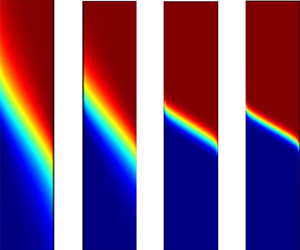
Figure 5(a) shows heat maps for  $\theta$ when $Ra=1,10,100$; from these, we see that there is a thermal boundary layer at the warm boundary for $Y<0$, and at the cold boundary for $Y>0$. This helps to explain the features seen in figure 3(b), namely that $\theta _{X}$ is large for $Y<0$, but practically zero for $Y>0$. In addition, the plots show the appearance of an interior layer as $Ra$ is increased, as discussed in § 4.2.2 and Appendix B; however, even at $Ra=100$, the layer is still some way off from being oriented horizontally, as suggested in Appendix B. Nevertheless, the fact that the isotherms in this interior layer are still visible in figure 5(a)(iii), whereas those in the thermal boundary layers are not, indicates that the results of the asymptotic analysis, which estimate the width of the interior layer and the vertical thermal boundary layers as being $O(Ra^{-1/3})$ and $O( Ra^{-1})$, respectively, are qualitatively correct.

Figure 5. (a) Heat map for  $\theta$; (b) heat map for $P$; (c) contours for $\psi$. For all plots: (i) $Ra=1$, (ii) $Ra=10$, (iii) $Ra=100$.
Figure 5(b) shows heat maps for  $P$ when $Ra=1,10,100$. In fact, these appear to be practically identical, with only minor adjustments in the interior near $Y=0$. Figure 5(c) shows contour plots for $\psi$ when $Ra=1,10,100$. Here also, the plots are very similar to each other. We comment here that although we have not included the velocity vector plots here, the vectors point from right to left for $Y>0$, and left to right for $Y<0$.
6.2. Comparison of asymptotic and numerical results
We can also note that although the problem becomes more nonlinear as  $Ra$ is increased, the profile for $\psi$ in figure 5(c) remains more or less unchanged. To explore this further, figure 6(a) shows $\psi$ at $X=0$ for $-Y_{\infty }\leq Y\leq Y_{\infty }$ for $Ra=1,10,100$, as well as the solution for $\psi ^{( 0) }$ from (4.13), which has been shifted by a constant so that $\psi ^{( 0) }( -1/2,-Y_{\infty }) =0$; figure 6(b) shows $U$ at $X=0$ for $-Y_{\infty }\leq Y\leq Y_{\infty }$ for the same values of $Ra$, as well as the solution for $U^{( 0) }$ from (4.15). Surprisingly, even though $\psi ^{( 0) }$ ought not to be relevant for this discussion, since it was obtained for the $Ra\ll 1$ regime, it turns out that it provides an adequate approximation for $\psi$ even outside of this regime, with even the curve for $Ra=100$ being indistinguishable from that for $\psi ^{( 0) }$; in a similar vein, away from $Y=0$, the isobars in figure 5(b) resemble the hyperbolae $XY=\textrm {constant}$ that are suggested by (4.14). Overall, this appears to be another example of an asymptotic result being numerically useful far beyond its nominal range of validity, as discussed by Crighton (Reference Crighton1994) and Andrianov & Awrejcewicz (Reference Andrianov and Awrejcewicz2005).


Moreover, the result for  $\psi$ suggests that $\psi ^{\prime }( Y) =-Y$, which would explain the linear behaviour of $U$ and $\theta _{X}$ at $X=1/2$ away from $Y=0$ in figure 4. With this in mind, figure 7 superimposes the curve for $-Ra\,Y$ over the data from figure 4; hence it is clear that there is very good agreement away from the interior layer near $Y=0$.

Figure 7. Comparison of numerical solutions for  $U$ and $\theta _{X}$ at $X=1/2$ when $Ra=100$ for $Y_{\infty }=5$ with $-Ra\,Y$.
A further comparison of the asymptotic and numerical solutions is given in figure 8, which shows  $\theta$ as a function of $X$ for $Y=-9$ and $-4.5$ in the vicinity of $X=1/2$ for $Ra=100$; note that the computation was carried out using $Y_{\infty }=10$, whereas for the asymptotic solution we have used (4.25), which yields
 \begin{equation} {\theta=e^{Ra\,Y\left( {1}/{2}-X\right) }-\tfrac{1}{2}.} \end{equation}
It is notable that the agreement in figure 8(a) for  $Y=-9$ is not particularly good, since the mesh is not adequately resolved for these values of $Ra$ and $Y$; in figure 8(b) for $Y=-4.5$, the agreement is excellent. These results reinforce the comments made in conjunction with figure 4.

Figure 8. Comparison of numerical and asymptotic solutions for  $\theta$ near $X=1/2$ when $Ra=100$ with $Y_{\infty }=10$ for (a) $Y=-9$, (b) $Y=-4.5$. The curves in (b) are more or less indistinguishable.
6.3. Stability
To determine whether the calculated steady states are stable, we used them as initial conditions in a 2-D initial value problem solver. Focusing on  $Ra=100$, we found that indeed the steady-state solution was recovered. However, to test this further, we also performed a run for $Ra=100$, but using the steady-state solution obtained for a much lower value of $Ra$ ( $=1$) as the initial condition. Once again, the steady-state solution for $Ra=100$ was recovered, suggesting that steady-state solutions up to at least this value of $Ra$ would indeed be stable to 2-D perturbations; however, in the interests of brevity, we have not included the corresponding heat maps for the temperature as it evolves with time.
It is beyond the scope here as to whether these solutions are stable to 3-D perturbations and whether or not there is a critical Rayleigh number above which these 2-D steady solutions would be linearly unstable.
7. Relevance and significance for breathing walls
As mentioned in § 1, the problem studied here is believed to be of relevance to breathing walls; we now examine this statement in more detail.
Breathing walls are more frequently linked to the concept of dynamic insulation, whereby fresh air from the outside is sucked into a building whose walls are made of a porous insulating layer, with the required pressure difference being provided by a fan. On its way through the pores, the fresh air is warmed by the heat conducting out through the material in the opposite direction, assuming that the outside surroundings are cooler than the interior of the building; in addition, the wall can act as a filter of airborne pollutants. As regards the porous material, one example is no-fines concrete, which is a cement-based mixture involving large aggregates only, i.e. gravel with an average diameter in the 6–12 mm range and having a highly interconnected porous matrix (Alongi et al. Reference Alongi, Angelotti and Mazzarella2021); other examples are mineral wool (Alongi et al. Reference Alongi, Angelotti and Mazzarella2021) and cellulose (Ascione et al. Reference Ascione, Bianco, De Stasio, Mauro and Vanoli2015).
However, in hindsight, the formulation that we have considered here appears to be more akin to diffusive insulation (Taylor, Cawthorne & Imbabi Reference Taylor, Cawthorne and Imbabi1996), in the sense that a pressure difference has been established across the porous material indirectly as a consequence of the temperature difference. As a result, this leads to the possibility of flow into the building at the lower part of the insulating layer, and flow out at the upper part; this is different to what one would expect in the case of dynamic insulation, where air flow would be into the building everywhere. As a consequence, the problem depends not only on the coordinate normal to the insulating layer, but also on the coordinate parallel to it, which is what we have seen in our solutions. Moreover, were the steady flow to become unstable at values of the Rayleigh number higher than those considered here, it is clear that this would lead to either a more complex, steady, inflow/outflow scenario or an entirely unsteady one; the latter would appear to be far removed from the desired situation that occurs for the case of dynamic insulation, and therefore unfavourable. Even all of the above comes with the caveat that the inside of a building is not always necessarily warmer than outside; typically, to a rough approximation, one expects the outside temperature to undergo daily periodic oscillations, with maxima and minima on either side of the constant indoor temperature (Alongi, Angelotti & Mazzarella Reference Alongi, Angelotti and Mazzarella2020; Alongi et al. Reference Alongi, Angelotti and Mazzarella2021).
8. Conclusions
This paper has revisited the problem of natural convection in a vertical porous slab bounded by two permeable planes, both of which are kept at uniform, although different, temperatures (Barletta Reference Barletta2015). On re-analysing the problem, it was demonstrated that there is no one-dimensional steady-state solution, contrary to the result given in Barletta (Reference Barletta2015). Two-dimensional solutions for the steady state were then obtained numerically using a pressure–temperature formulation for values of  $Ra$ as high as $10^{2}$; the main characteristics of the flow were backed up, both qualitatively and quantitatively, by asymptotic analysis. Furthermore, the analysis given here would have implications for the results in Barletta (Reference Barletta2016), Celli et al. (Reference Celli, Barletta and Rees2017), Barletta & Celli (Reference Barletta and Celli2018) and Barletta & Rees (Reference Barletta and Rees2019), wherein pressure boundary conditions at permeable boundaries were considered and one-dimensional steady-state solutions for the base flow were found and used for stability analyses. We also performed 2-D transient computations and found that the steady-state solutions for $Ra$ as high as $10^{2}$ would be stable to 2-D perturbations.
Acknowledgements
The authors would like to thank the anonymous reviewers for their invaluable comments and suggestions.
Declaration of interests
The authors report no conflict of interest.
Appendix A. Boundary conditions (2.6) and (2.7)
Here, we consider how boundary conditions (2.6) and (2.7) can be arrived at from a more general model that takes into account the field equations for both the insulation layer and the reservoirs. Without loss of generality, we will consider only (2.7).
In order to avoid having to discuss the complications associated with the Beavers–Joseph conditions at the interface of a porous medium and a clear fluid (Beavers & Joseph Reference Beavers and Joseph1967; Ochoa-Tapia & Whitaker Reference Ochoa-Tapia and Whitaker1995a,Reference Ochoa-Tapia and Whitakerb, Reference Ochoa-Tapia and Whitaker1998a,Reference Ochoa-Tapia and Whitakerb; Jager & Mikelic Reference Jäger and Mikelic2000), we assume for simplicity that the reservoir is itself a porous medium, having permeability  $\kappa _{res}$, where $\kappa _{res}\gg \kappa$, and porosity $\phi _{res}$, where $\phi _{res}>\phi$; in addition, let $k_{res}$ denote the thermal conductivity of the solid matrix of this porous medium. In the reservoir, the velocity, pressure and temperature fields satisfy (2.1)–(2.4), with the physical parameters replaced accordingly, whereas far from the interface at $x=L/2$, we can reasonably suppose that
 \begin{equation} {p\rightarrow p_{h},\quad T\rightarrow T_{2}.} \end{equation}
At  $x=L/2$, we would expect the continuity of pressure, continuity of normal velocity, continuity of temperature, and continuity of normal heat flux; thus, respectively,
 \begin{gather} {\left[ p\right] _{-}^{+}} {=0,} \end{gather}
 \begin{gather}{-\frac{\kappa}{\mu}\left( \frac{\partial p}{\partial x}\right) _{-}} {={-}\frac{\kappa_{res}}{\mu}\left( \frac{\partial p}{\partial x}\right) _{+},} \end{gather}
 \begin{gather}{\left[ T\right] _{-}^{+}} {=0,} \end{gather}
 \begin{gather}{-\left( \left[ \left( 1-\phi\right) k_{s}+\phi k\right] \frac{\partial T}{\partial x}\right) _{-}} {={-}\left( \left[ \left( 1-\phi _{res}\right) k_{res}+\phi_{res}k\right] \frac{\partial T}{\partial x}\right) _{+},} \end{gather}
with  $[ \textrm { \ }] _{-}^{+}$ denoting the difference in the value of a function above and below $x=L/2$, and $( \textrm { \ }) _{\pm }$ denoting the value of a function in the limit as $x$ tends to $L/2$ from above and below, respectively.
Now, since  $\kappa _{res}\gg \kappa$, (A3) reduces to
 \begin{equation} {\left( \frac{\partial p}{\partial x}\right) _{+}\approx0;} \end{equation}
moreover, (A5) reduces to
 \begin{equation} {\left( \frac{\partial T}{\partial x}\right) _{+}\approx0} \end{equation}
if  $( 1-\phi _{res}) k_{res}+\phi _{res}k\gg ( 1-\phi ) k_{s}+\phi k$. Thence, with (A6) and (A7) as boundary conditions at $x=L/2$, it is clear that $p\approx p_{h}$, $T\approx T_{2}$ for the reservoir, which then leads to (2.7), as required.
Appendix B. Interior layer for $Ra\gg 1$

Supposing that  $\psi =0$ on $Y=0$, and that the interior layer is of width $O( \epsilon )$, where $\epsilon \ll 1$ and is to be determined, we may at least be able to make an estimate for $\epsilon$ in terms of $Ra$. Supposing that $\psi \sim [ \psi ]$, where $[ \psi ]$ is also to be determined, we set
 \begin{equation} Y=\epsilon\eta,\quad\psi=\left[ \psi\right] \varPsi, \end{equation}
so that (4.2) and (4.3) become, at leading order,
 \begin{gather} \frac{\left[ \psi\right] }{\epsilon^{2}}\,\varPsi_{\eta\eta} ={-}\theta_{X}, \end{gather}
 \begin{gather}\frac{\left[ \psi\right] }{\epsilon}\left( \varPsi_{\eta}\theta_{X}-\varPsi _{X}\theta_{\eta}\right) =\frac{1}{Ra\,\epsilon^{2}}\,\theta_{\eta\eta}. \end{gather}
Hence (B2) and (B3) suggest that
 \begin{equation} \left[ \psi\right] \sim\epsilon^{2},\quad\frac{\left[ \psi\right] }{\epsilon}\sim\frac{1}{Ra\,\epsilon^{2}}, \end{equation}
leading to
 \begin{equation} \epsilon\sim Ra^{{-}1/3},\quad\left[ \varPsi\right] \sim Ra^{{-}2/3}. \end{equation}
So the problem at hand is, for  $-\infty <\eta <\infty$ and $-1/2\leq X\leq 1/2$,
 \begin{gather} \varPsi_{\eta\eta} ={-}\theta_{X}, \end{gather}
 \begin{gather}\varPsi_{\eta}\theta_{X}-\varPsi_{X}\theta_{\eta} =\theta_{\eta\eta}, \end{gather}
subject to boundary conditions as  $\eta \rightarrow \pm \infty$, as well as initial-like conditions for $\theta$, since (B7) contains a term in $\theta _{X}$, where $X$ plays the role of a time-like variable. The boundary conditions for $\theta$ seem to be fairly straightforward and are just
 \begin{equation} \theta\rightarrow\pm\tfrac{1}{2}\quad\text{as }\eta\rightarrow\pm\infty. \end{equation}
As regards  $\varPsi$, (B6) and (B8) suggest that $\varPsi _{\eta \eta }\rightarrow 0$ as $\eta \rightarrow \pm \infty$, from which we might infer that $\varPsi _{\eta }$ should, in general, tend to different functions of $X$ as $\eta \rightarrow \pm \infty$, although it is not clear at present how these functions would be determined; indeed, we cannot even rule out the simplest possibility that just $\varPsi _{\eta }\rightarrow 0$ as $\eta \rightarrow \pm \infty$. The initial-like conditions are even less straightforward. In view of the orientation of the velocity vectors, which can be inferred from figure 5(c) and indicate $\psi _{Y}>0$ for $Y<0$ and $\psi _{Y}<0$ for $Y>0$, we can surmise that there should be one condition for $\theta$ at $X=-1/2$ for $\eta \leq 0$ and another at $X=1/2$ for $\eta \geq 0$; moreover, no initial-like conditions are required on $\varPsi$, since there are no $X$-derivatives of $\varPsi$ in (B6). In fact, the situation is similar to that in Fowler & Robinson (Reference Fowler and Robinson2018) for flow in a volcanic conduit, in that we have counter-current convection in a thin layer; in that case, there was no equivalent of (B6) and $\varPsi =-\eta ^{2}/2$, meaning that a solution for $\theta$ could be found by using Laplace transforms and solving a resulting integral equation, as originally done in Carrier, Krook & Pearson (Reference Carrier, Krook and Pearson1966) and Howard & Veronis (Reference Howard and Veronis1987), so as to determine $\theta ( X,0)$. Of course, the current problem is nonlinear and there is no possibility of finding a solution by Laplace transforms. Moreover, these initial-like conditions should reflect what is coming from the vertical boundaries at $X=\pm 1/2$, which would require us to consider more closely what happens in the vicinity of $( -1/2,0)$ and $( 1/2,0)$.
Consider, without loss of generality, the point  $( -1/2,0)$. For the boundary layer near $X=-1/2$ for $Y>0$, we have $X+1/2\sim Ra^{-1}$, and in the vicinity of $( -1/2,0)$ we could reasonably expect that $X+1/2\sim Y$. Supposing then that $X+1/2\sim \varDelta$, $Y\sim \varDelta$, where $\varDelta ( \ll 1)$ is to be determined, (4.2) and (4.3) would give, on setting $X+1/2=\varDelta \bar {X}$ and $Y=\varDelta \bar {Y}$,
 \begin{gather} \psi_{\bar{X}\bar{X}}+\psi_{\bar{Y}\bar{Y}} ={-}\varDelta\theta_{\bar{X}}, \end{gather}
 \begin{gather}\psi_{\bar{Y}}\theta_{\bar{X}}-\psi_{\bar{X}}\theta_{\bar{Y}} =\frac {1}{Ra}\left( \theta_{\bar{X}\bar{X}}+\theta_{\bar{Y}\bar{Y}}\right) , \end{gather}
respectively. This would imply that we have self-consistency if  $\psi \sim \varDelta$ and $\varDelta =1/Ra$, with all second derivatives being retained and it therefore being possible to satisfy all boundary conditions at $\bar {X}=0$ and $\bar {Y}\rightarrow \pm \infty$, as well as matching conditions as $\bar {X}\rightarrow \pm \infty$. This would mean that the extent of this region in the $Y$-direction, $Ra^{-1}$, is much smaller than the extent of the interior layer in the $Y$-direction, $Ra^{-1/3}$. In turn, this suggests that near $X=-1/2$, the interior layer merely sees the value of $\theta$ at the lower outer edge of this $O( Ra^{-1}) \times O( Ra^{-1})$ region, i.e. $\theta =-1/2$ for $\eta \leq 0$. Using an analogous argument near $X=1/2$ for $\eta \geq 0$, we would obtain the following initial-like conditions:
 \begin{equation} \theta=\left\{ \begin{array}{@{}ll} -1/2, & X={-}1/2,\text{ for }\eta\leq0,\\ 1/2, & X=1/2,\text{ for }\eta\geq0. \end{array} \right. \end{equation}
The reason for not using the upper outer edge near  $X=-1/2$ and the lower outer edge near $X=1/2$ is to do with the direction of the flow, as discussed in the previous paragraph.
The above considerations are summarized schematically in figures 9 and 10. Figure 9 shows how the suggested interior layer and the  $O( Ra^{-1}) \times O( Ra^{-1})$ regions near $( -1/2,0)$ and $( 1/2,0)$ fit into the overall asymptotic structure of the problem, whereas figure 10 indicates the structure of the interior layer. Finding solutions of (B6) and (B7), subject to (B8), (B11) and a suitable condition on $\varPsi _{\eta }$ as $\eta \rightarrow \pm \infty$, constitutes an interesting, but challenging, numerical task, although the result will not affect the earlier work in this paper.

Figure 9. Asymptotic structure of the problem as  $Ra\rightarrow \infty$.

Figure 10. Structure of the interior layer, with boundary and initial-like conditions for  $\theta$.


 Open access