


1 Introduction
Horizontal convection (HC) is convection generated in a fluid layer  $0<z<h$ by imposing non-uniform buoyancy along the top surface
  $z=h$; all other bounding surfaces are insulated (Sandström Reference Sandström1908; Rossby Reference Rossby1965; Hughes & Griffiths Reference Hughes and Griffiths2008). The problem of HC is a basic one in fluid mechanics and serves as an interesting counterpoint to the much more widely studied problem of Rayleigh–Bénard convection (RBC) in which the fluid layer is heated at the bottom,
  $z=0$, and cooled the top,
  $z=h$.
In RBC the correct definition of the Nusselt number,  $Nu$, is clear: after averaging over
  $(x,y,t)$ there is a constant vertical heat flux passing through every level of constant
  $z$ between
  $0$ and
  $h$. By definition, the RBC
  $Nu$ is the constant vertical heat flux through the layer divided by the diffusive heat flux of the unstable static solution.
In HC, however, there is zero net vertical heat flux through every level of constant  $z$. Thus, using notation introduced systematically in § 3, if the vertical flux of buoyancy or heat through the non-uniform surface is denoted by
  $F(x)$ then
  $\overline{F}=0$, where the overline denotes an
  $x$-average. To obtain a non-zero index of the vertical heat flux, Rossby (Reference Rossby1965, Reference Rossby1998) defined the Nusselt number of HC as a suitably normalized version of
  $\overline{|F|}$. In § 3 we discuss three other definitions of the horizontal-convective
  $Nu$, and recommend
 $$\begin{eqnarray}Nu\stackrel{\text{def}}{=}\unicode[STIX]{x1D712}/\unicode[STIX]{x1D712}_{diff}\end{eqnarray}$$
 as the best of the four. In (1.1),  $\unicode[STIX]{x1D712}$ is the dissipation of buoyancy (or thermal) variance defined in (3.7) below and
  $\unicode[STIX]{x1D712}_{diff}$ is the corresponding quantity of the diffusive (i.e. zero Rayleigh number) solution. In the context of RBC, Howard (Reference Howard1963) remarked that
  $\unicode[STIX]{x1D712}$ is a measure of the entropy production by thermal diffusion within the enclosure; in this work, we explore the ramifications of viewing (1.1) as a measure of HC entropy production.
The ratio on the right-hand side of (1.1) was introduced as a non-dimensional index of the strength of HC by Paparella & Young (Reference Paparella and Young2002). But because there seemed to be no clear connection to heat flux, Paparella & Young (Reference Paparella and Young2002) did not refer to  $\unicode[STIX]{x1D712}/\unicode[STIX]{x1D712}_{diff}$ as a ‘Nusselt number’. The ratio
  $\unicode[STIX]{x1D712}/\unicode[STIX]{x1D712}_{diff}$ has been used as an index of HC in a few subsequent papers (Siggers, Kerswell & Balmforth Reference Siggers, Kerswell and Balmforth2004; Rocha et al. Reference Rocha, Bossy, Llewellyn Smith and Young2020). But most authors prefer to work with a Nusselt number with a more obvious connection to the heat flux. In § 3 we address this concern by establishing relations between
  $Nu$ in (1.1) and the horizontal and vertical heat fluxes in HC. This justifies referring to
  $\unicode[STIX]{x1D712}/\unicode[STIX]{x1D712}_{diff}$ as a Nusselt number, and we note other advantages that compel (1.1) as the best definition of a horizontal-convective Nusselt number.
Section 4 discusses the transient adjustment of  $Nu$ in (1.1) to its long-time average and introduces a ‘surface Nusselt number’,
  $Nu_{s}$, that is defined in terms of the entropy flux through the top surface. In statistical steady state the surface flux of entropy must balance the interior production of entropy and so, with sufficient time averaging,
  $Nu_{s}=Nu$. The Nusselt number
  $Nu_{s}$ has the advantage of requiring only a surface integral, rather than the volume integral of
  $|\unicode[STIX]{x1D735}b|^{2}$ involved in (1.1). In § 4 we also discuss the quantitative differences between the
  $\unicode[STIX]{x1D712}$-based
  $Nu$ in (1.1) and Rossby’s Nusselt number based on
  $\overline{|F|}$. Section 5 is the conclusion.
2 Formulation of the HC problem
Consider a Boussinesq fluid with density  $\unicode[STIX]{x1D70C}=\unicode[STIX]{x1D70C}_{0}(1-g^{-1}b)$, where
  $\unicode[STIX]{x1D70C}_{0}$ is a constant reference density,
  $b$ is the ‘buoyancy’ and
  $g$ is the gravitational acceleration. If the fluid is stratified by temperature variations then
  $b=g\unicode[STIX]{x1D6FC}(T-T_{0})$, where
  $T_{0}$ is a reference temperature and
  $\unicode[STIX]{x1D6FC}$ is the thermal expansion coefficient. The Boussinesq equations of motion are
 $$\begin{eqnarray}\displaystyle & \displaystyle \boldsymbol{u}_{t}+\boldsymbol{u}\boldsymbol{\cdot }\unicode[STIX]{x1D735}\boldsymbol{u}+\unicode[STIX]{x1D735}p=b\hat{\boldsymbol{z}}+\unicode[STIX]{x1D708}\unicode[STIX]{x1D6FB}^{2}\boldsymbol{u}, & \displaystyle\end{eqnarray}$$
 $$\begin{eqnarray}\displaystyle & \displaystyle b_{t}+\boldsymbol{u}\boldsymbol{\cdot }\unicode[STIX]{x1D735}b=\unicode[STIX]{x1D705}\unicode[STIX]{x1D6FB}^{2}b, & \displaystyle\end{eqnarray}$$
 $$\begin{eqnarray}\displaystyle & \displaystyle \unicode[STIX]{x1D735}\boldsymbol{\cdot }\boldsymbol{u}=0. & \displaystyle\end{eqnarray}$$
 The kinematic viscosity is  $\unicode[STIX]{x1D708}$ and the thermal diffusivity is
  $\unicode[STIX]{x1D705}$.
2.1 Horizontal-convective boundary conditions and control parameters
We suppose the fluid occupies a rectangular domain with depth  $h$, length
  $\ell _{x}$ and width
  $\ell _{y}$; we assume periodicity in the horizontal directions,
  $x$ and
  $y$. At the bottom surface (
 $z=0$) and top surface
  $(z=h)$ the boundary conditions on the velocity
  $\boldsymbol{u}=(u,v,w)$ are
  $w=0$ and for the viscous boundary condition either no slip,
  $u=v=0$, or free slip,
  $u_{z}=v_{z}=0$. At
  $z=0$ the buoyancy boundary condition is no flux,
  $\unicode[STIX]{x1D705}b_{z}=0$; at the top,
  $z=h$, the boundary condition is
  $b=b_{s}(x)$, where the top surface buoyancy
  $b_{s}$ is a prescribed function of
  $x$. As a surface buoyancy field we use
 $$\begin{eqnarray}b_{s}(x)=b_{\star }\cos (kx),\end{eqnarray}$$
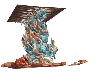
 where  $k\stackrel{\text{def}}{=}2\unicode[STIX]{x03C0}/\ell _{x}$. Figure 1 shows a three-dimensional (3-D) HC flow with no-slip boundary conditions and the surface buoyancy (2.4). Figure 2 shows
  $y$-averaged buoyancy and the overturning streamfunction calculated by
  $y$-averaging the 3-D velocity. These figures illustrate three main large-scale features of HC: a buoyancy boundary layer pressed against the non-uniform upper surface and uniform buoyancy in the deep bulk; an entraining plume beneath the densest point on the upper surface; and interior upwelling towards the non-uniform surface in the bulk of the domain.

Figure 1. A snapshot of the  $b=-0.7964b_{\star }$ surface at
  $\unicode[STIX]{x1D705}t/h^{2}=0.12$ for a 3-D horizontal-convective flow; colours denote the vertical velocity. This is a no-slip solution with sinusoidal surface buoyancy
  $b_{s}$ in (2.4); control parameters are
  $Ra=6.4\times 10^{10}$,
  $Pr=1$,
  $A_{x}=4$ and
  $A_{y}=1$.

Figure 2. Snapshots of (a) streamfunction, calculated from the  $y$-averaged velocity (
 $u$,
$u$,  $w$), and (b) the
  $y$-averaged buoyancy at
  $\unicode[STIX]{x1D705}t/h^{2}=0.12$. This is the same solution as that of figure 1. The streamfunction in (a) is defined by the
  $y$-average of
  $u$ and
  $w$. The black contour in (b) is
  $b=-0.79b_{\star }$, which is close to the bottom buoyancy, defined as the
  $(x,y,t)$-average of
  $b$ at
  $z=0$.
The problem is characterized by four non-dimensional parameters: the Rayleigh and Prandtl numbers
 $$\begin{eqnarray}Ra\stackrel{\text{def}}{=}\frac{\ell _{x}^{3}b_{\star }}{\unicode[STIX]{x1D708}\unicode[STIX]{x1D705}}\quad \text{and}\quad Pr\stackrel{\text{def}}{=}\frac{\unicode[STIX]{x1D708}}{\unicode[STIX]{x1D705}},\end{eqnarray}$$
 and the aspect ratios  $A_{x}\stackrel{\text{def}}{=}\ell _{x}/h$ and
  $A_{y}\stackrel{\text{def}}{=}\ell _{y}/h$. Two-dimensional (2-D) HC corresponds to
  $A_{y}=0$.
2.2 Horizontal-convective power integrals
We use an overline  $\overline{\,\cdots \,}$ to denote an average over
  $x$,
$x$,  $y$ and
  $t$, taken at any fixed
  $z$, and angle brackets
  $\langle \cdots \rangle$ to denote a total volume average over
  $x$,
$x$,  $y$,
$y$,  $z$ and
  $t$. Using this notation, we recall some results from Paparella & Young (Reference Paparella and Young2002) that are used below.
Horizontally averaging the buoyancy equation (2.2), we obtain the zero-flux constraint
 $$\begin{eqnarray}\overline{wb}-\unicode[STIX]{x1D705}\bar{b}_{z}=0.\end{eqnarray}$$
Forming 〈u⋅ (2.1)〉, we obtain the kinetic energy power integral
 $$\begin{eqnarray}\unicode[STIX]{x1D700}=\langle wb\rangle ,\end{eqnarray}$$
 where  $\unicode[STIX]{x1D700}\stackrel{\text{def}}{=}\unicode[STIX]{x1D708}\langle |\unicode[STIX]{x1D735}\boldsymbol{u}|^{2}\rangle$ is the rate of dissipation of kinetic energy and
  $\langle wb\rangle$ is the rate of conversion between potential and kinetic energy.
Vertically integrating (2.6) from  $z=0$ to
  $h$ we obtain another expression for
  $\langle wb\rangle$; substituting this into (2.7) we find
 $$\begin{eqnarray}\unicode[STIX]{x1D700}=\unicode[STIX]{x1D705}\unicode[STIX]{x0394}\bar{b}/h,\end{eqnarray}$$
 where  $\unicode[STIX]{x0394}\bar{b}=\bar{b}(h)-\bar{b}(0)$ is the difference between the
  $(x,y,t)$-average of the buoyancy at the top,
  $z=h$, and the buoyancy at the bottom,
  $z=0$. The buoyancy difference can be bounded using the extremum principle for the buoyancy advection–diffusion equation (2.2). In the case of the sinusoidal profile in (2.4), with
  $\bar{b}(h)=0$, this leads to the inequality
 $$\begin{eqnarray}\unicode[STIX]{x1D700}\leqslant \unicode[STIX]{x1D705}b_{\star }/h.\end{eqnarray}$$
 In the example shown in figure 1 the bottom buoyancy is  $\bar{b}(0)\approx -0.83b_{\star }$ and thus the right-hand side of inequality (2.9) is about 20 % larger than
  $\unicode[STIX]{x1D700}$.
3 Definition of the horizontal-convective Nusselt number
For equilibrated HC the vertical buoyancy flux is zero through every level – see (2.6) – and cannot be used to define a Nusselt number analogous to that of RBC. Moreover, with specified  $b_{s}(x)$, buoyancy is transported along the
  $x$ axis and it is natural to consider the net horizontal flux,
 $$\begin{eqnarray}J(x)\stackrel{\text{def}}{=}\frac{1}{\unicode[STIX]{x1D70F}h\ell _{y}}\int _{0}^{\unicode[STIX]{x1D70F}}\int _{0}^{\ell _{y}}\int _{0}^{h}(ub-\unicode[STIX]{x1D705}b_{x})\,\text{d}z\,\text{d}y\,\text{d}t,\end{eqnarray}$$
 in defining an HC Nusselt number. In (3.1)  $\unicode[STIX]{x1D70F}$ is a time horizon sufficiently long so that the time average removes unsteady fluctuations remaining after the spatial average over the
  $(y,z)$ plane. But
  $J(x)$ is not constant and it is not initially obvious how to best define a single number out of
  $J(x)$ as an index of HC buoyancy transport.
Another measure of horizontal-convective transport is provided by the averaged vertical buoyancy flux through the non-uniformly heated surface at  $z=h$:
 $$\begin{eqnarray}F(x)\stackrel{\text{def}}{=}\frac{1}{\unicode[STIX]{x1D70F}\ell _{y}}\int _{0}^{\unicode[STIX]{x1D70F}}\int _{0}^{\ell _{y}}\unicode[STIX]{x1D705}b_{z}(x,y,h,t)\,\text{d}y\,\text{d}t.\end{eqnarray}$$
 Averaging the buoyancy equation (2.2) over the  $(y,z)$ plane, and also over time, one finds that the divergence of the
  $x$ flux in (3.1) is equal to the flux in and out through the top:
 $$\begin{eqnarray}h\frac{\text{d}J}{\text{d}x}=F.\end{eqnarray}$$
 Figure 3 exhibits the functions  $J(x)$ and
  $F(x)$ for the
  $Ra=6.4\times 10^{10}$ solution shown in figure 1.

Figure 3. (a) The dashed black curve is the sinusoidal surface buoyancy profile in (2.4) and the solid blue curve is the vertical flux  $F(x)$ defined in (3.2). (b) The horizontal flux
  $J(x)$ defined in (3.1) (the solid blue curve) and the relation (3.14) with
  $D$ diagnosed from (3.17) (the dashed black curve). This is the same solution as that of figures 1 and 2.
3.1 Two horizontal-convective Nusselt numbers
Following Rossby (Reference Rossby1965, Reference Rossby1998), some authors use, more or less, the Nusselt number
 $$\begin{eqnarray}Nu_{F}\stackrel{\text{def}}{=}\overline{|F|}/\overline{|F_{diff}|}.\end{eqnarray}$$
 In (3.4),  $F_{diff}$ is the vertical flux of the diffusive solution, i.e. the vertical buoyancy flux produced by the solution of
  $\unicode[STIX]{x1D6FB}^{2}b_{diff}=0$, with
  $b_{diff}$ satisfying the same boundary conditions as
  $b$ (e.g. Chiu-Webster, Hinch & Lister Reference Chiu-Webster, Hinch and Lister2008; Tsai et al. Reference Tsai, Hussam, King and Sheard2020). We say ‘more or less’ because in practice the normalizing denominator
  $\overline{|F_{diff}|}$ in (3.4) is sometimes replaced with a scale estimate such as
  $\unicode[STIX]{x1D705}b_{\star }/\ell _{x}$.
As a variant of (3.4), other authors define a Nusselt number based on the net buoyancy flux through that part of the non-uniformly heated surface with a destabilizing vertical buoyancy flux, i.e. that part of the surface where  $F(x)<0$ (e.g. Hughes & Griffiths Reference Hughes and Griffiths2008; Gayen et al. Reference Gayen, Griffiths, Hughes and Saenz2013; Gayen, Griffiths & Hughes Reference Gayen, Griffiths and Hughes2014; Rosevear, Gayen & Griffiths Reference Rosevear, Gayen and Griffiths2017). Let
  $X^{-}$ denote that part of the non-uniformly heated surface where
  $F=-|F|<0$ and
  $X^{+}$ that part where
  $F=+|F|>0$. Because there is no net flux through the surface
 $$\begin{eqnarray}\int _{X_{-}}F(x)\,\text{d}x+\int _{X_{+}}F(x)\,\text{d}x=0,\end{eqnarray}$$
and so
 $$\begin{eqnarray}\int _{X_{-}}|F(x)|\,\text{d}x=\int _{X_{+}}F(x)\,\text{d}x={\textstyle \frac{1}{2}}\ell _{x}\overline{|F|}.\end{eqnarray}$$
 Despite the close connection between the relation above and the numerator on the right-hand side of (3.4), this alternative Nusselt number is not simply related to  $Nu_{F}$: one must normalize the
  $X_{-}$ integral in (3.6) by the length of the interval
  $X_{-}$. This unknown length varies with
  $Ra$ and is not equal to
  $\ell _{x}/2$ – though in figure 3(a) it is close. Hence a priori there is not a simple relation between
  $Nu_{F}$ and the Nusselt number based on the destabilized part of the boundary.
Siggers et al. (Reference Siggers, Kerswell and Balmforth2004) considered, and rejected, the Nusselt numbers discussed above as too difficult for theoretical work. The problem is that one does not know in advance where buoyancy flows into and out of the domain and it is difficult to get an analytic grip on  $|F|$. As an indication of the difficulty, there is no proof that the two
  $F$-based Nusselt numbers discussed above, when correctly normalized by the diffusive solution, are strictly greater than one. One expects on physical grounds that any fluid motion must increase buoyancy transport above that of the diffusive solution. A good definition of Nusselt number should manifestly satisfy this basic requirement and the Nusselt numbers above do not.
3.2 The Nusselt number  $Nu\stackrel{\text{def}}{=}\unicode[STIX]{x1D712}/\unicode[STIX]{x1D712}_{diff}$ and some of its properties

The alternative to the Nusselt numbers discussed above is to use the diffusive dissipation of buoyancy variance,
 $$\begin{eqnarray}\unicode[STIX]{x1D712}\stackrel{\text{def}}{=}\unicode[STIX]{x1D705}\langle |\unicode[STIX]{x1D735}b|^{2}\rangle ,\end{eqnarray}$$
 and define the Nusselt number as in (1.1) (Paparella & Young Reference Paparella and Young2002; Siggers et al. Reference Siggers, Kerswell and Balmforth2004; Rocha et al. Reference Rocha, Bossy, Llewellyn Smith and Young2020). It is straightforward to show that  $Nu$ in (1.1) is greater than unity: amongst all functions
  $c(\boldsymbol{x})$ that satisfy the same boundary conditions as
  $b(\boldsymbol{x},t)$, the diffusive solution
  $b_{diff}(\boldsymbol{x})$ minimizes the functional
  $\langle |\unicode[STIX]{x1D735}c|^{2}\rangle$.
Now  $\unicode[STIX]{x1D712}$ in (3.7) does not have an obvious connection to the fluxes
  $J(x)$ and
  $F(x)$ in (3.1) and (3.2). This is probably why
  $\unicode[STIX]{x1D712}/\unicode[STIX]{x1D712}_{diff}$ has not been popular as an index of the strength of HC. Siggers et al. (Reference Siggers, Kerswell and Balmforth2004) refer to
  $\unicode[STIX]{x1D712}$ as a ‘pseudo-flux’ because
  $\unicode[STIX]{x1D712}$ seems not to have a clear connection to the horizontal flux
  $J(x)$. But in (3.9) below, we establish an integral relation between
  $\unicode[STIX]{x1D712}$ and
  $J$: this supports
  $\unicode[STIX]{x1D712}/\unicode[STIX]{x1D712}_{diff}$ as a useful definition of
  $Nu$.
$Nu$.
Multiplying the buoyancy equation (2.2) with  $b$ and taking the total volume–time average
  $\langle \rangle$ we obtain a ‘power integral’ that expresses
  $\unicode[STIX]{x1D712}$ entirely in terms of conditions at the non-uniform surface
  $z=h$:
 $$\begin{eqnarray}\unicode[STIX]{x1D712}=\overline{Fb_{s}}/h,\end{eqnarray}$$
 where  $F(x)$ is the vertical buoyancy flux in (3.2) and
  $b_{s}(x)$ is the non-uniform surface buoyancy. Noting that
  $\unicode[STIX]{x1D712}>0$, we see that (3.8) has an intuitive physical interpretation: on average buoyancy enters the domain (
 $F(x)>0$) where
  $b_{s}(x)$ is higher than its average value and leaves (
 $F(x)<0$) at locations where
  $b_{s}(x)$ is lower than its average value. In § 4.3 we discuss further useful properties of the buoyancy power integral (3.8).
Using (3.3) to replace  $F$ in (3.8) by
  $\text{d}J/\text{d}x$, and integrating by parts in
  $x$, one finds
 $$\begin{eqnarray}\unicode[STIX]{x1D712}=-\overline{J\frac{\text{d}b_{s}}{\text{d}x}}.\end{eqnarray}$$
 Thus  $\unicode[STIX]{x1D712}$ is directly related to an
  $x$-average of
  $J(x)$, weighted by the surface buoyancy gradient: in this sense
  $\unicode[STIX]{x1D712}$ is a bulk index of the horizontal buoyancy flux of HC. The relation (3.9) also shows that the horizontal flux
  $J$ is, on average, down the applied surface gradient
  $\text{d}b_{s}/\text{d}x$. Below in (3.16) we use (3.9) to define an intuitive ‘effective diffusivity’ of HC.
3.3 The Nusselt number of a discontinuous surface buoyancy profile
There is a fourth definition of the HC Nusselt number which, however, only applies to piecewise constant surface forcing profiles, such as
 $$\begin{eqnarray}b_{s}(x)=\left\{\begin{array}{@{}ll@{}}+b_{\star },\quad & \text{for }-\ell _{x}/2<x<0;\\ -b_{\star },\quad & \text{for }0<x<+\ell _{x}/2\end{array}\right.\end{eqnarray}$$
 (Shishkina, Grossmann & Lohse Reference Shishkina, Grossmann and Lohse2016; Passaggia, Scotti & White Reference Passaggia, Scotti and White2017). The advantage of the profile (3.10) is that the horizontal buoyancy flux through the discontinuity in  $b_{s}(x)$ – that is
  $J(0)$ – is distinguished and provides a ‘natural’ definition of the horizontal-convective Nusselt number.
Now with the discontinuous  $b_{s}(x)$ in (3.10), the surface buoyancy gradient is
  $2b_{\star }\unicode[STIX]{x1D6FF}(x)$ and (3.9) is particularly simple:
 $$\begin{eqnarray}\unicode[STIX]{x1D712}=-2b_{\star }J(0)/\ell _{x}.\end{eqnarray}$$
 For the special  $b_{s}(x)$ in (3.10) there is a direct connection between
  $\unicode[STIX]{x1D712}$ and the flux through the location of the discontinuous jump in buoyancy, i.e. the
  $\unicode[STIX]{x1D712}$-based definition of
  $Nu$ in (1.1) recovers the natural definition of Nusselt number associated with the discontinuous
  $b_{s}$ in (3.10). Of course,
  $Nu$ in (1.1) is not restricted to piecewise constant surface forcing profiles, but can also be applied to smoothly varying
  $b_{s}(x)$ such as the sinusoid in (2.4), or to the case with constant
  $\text{d}b_{s}/\text{d}x$ (Rossby Reference Rossby1965; Sheard & King Reference Sheard and King2011).
3.4 Two-dimensional surface buoyancy distributions and the effective diffusivity
The  $Nu$ in (1.1) copes with 2-D surface buoyancy distributions,
  $b_{s}(x,y)$, such as the examples considered by Rosevear et al. (Reference Rosevear, Gayen and Griffiths2017). In this case, and in analogy with (3.1), one can define a 2-D buoyancy flux,
  $\boldsymbol{J}$, as the
  $(z,t)$ average of
  $(ub-\unicode[STIX]{x1D705}b_{x})\hat{\boldsymbol{x}}+(vb-\unicode[STIX]{x1D705}b_{y})\hat{\boldsymbol{y}}$. Then it is easy to show that the generalizations of (3.3) and (3.9) are
 $$\begin{eqnarray}h\,\unicode[STIX]{x1D735}\!\boldsymbol{\cdot }\!\,\boldsymbol{J}=F\end{eqnarray}$$
and
 $$\begin{eqnarray}\overline{\boldsymbol{J}\boldsymbol{\cdot }\unicode[STIX]{x1D735}b_{s}}=-\unicode[STIX]{x1D712}.\end{eqnarray}$$
 Thus the horizontal buoyancy flux  $\boldsymbol{J}$ is, on average, down the applied surface buoyancy gradient
  $\unicode[STIX]{x1D735}b_{s}$, and
  $\unicode[STIX]{x1D712}$ emerges as a measure of this horizontal-convective transport.
The down-gradient direction of  $\boldsymbol{J}$ suggests a relation between
  $\boldsymbol{J}$ and
  $\unicode[STIX]{x1D735}b_{s}$ in terms of an ‘effective diffusivity’,
  $D$. Thus we propose that
 $$\begin{eqnarray}\boldsymbol{J}\approx -D\unicode[STIX]{x1D735}b_{s},\end{eqnarray}$$
 where  $D$ is a constant. An estimate of
  $D$ is obtained by minimizing the squared error
 $$\begin{eqnarray}E(D)\stackrel{\text{def}}{=}\overline{|\boldsymbol{J}+D\unicode[STIX]{x1D735}b_{s}|^{2}}.\end{eqnarray}$$
 Setting  $\text{d}E/\text{d}D$ to zero we obtain
 $$\begin{eqnarray}D\stackrel{\text{def}}{=}-\overline{\boldsymbol{J}\boldsymbol{\cdot }\unicode[STIX]{x1D735}b_{s}}/\overline{|\unicode[STIX]{x1D735}b_{s}|^{2}}.\end{eqnarray}$$
 Substituting (3.13) into (3.16), the effective diffusivity, defined via minimization of  $E(D)$, is diagnosed as
 $$\begin{eqnarray}\displaystyle D & = & \displaystyle \unicode[STIX]{x1D705}\left\langle |\unicode[STIX]{x1D735}b|^{2}\right\rangle /\overline{|\unicode[STIX]{x1D735}b_{s}|^{2}}\end{eqnarray}$$
 $$\begin{eqnarray}\displaystyle & = & \displaystyle Nu\,\unicode[STIX]{x1D705}\langle |\unicode[STIX]{x1D735}b_{diff}|^{2}\rangle /\overline{|\unicode[STIX]{x1D735}b_{s}|^{2}}.\end{eqnarray}$$
 In (3.17) the ratio  $\left\langle |\unicode[STIX]{x1D735}b|^{2}\right\rangle /\,\overline{|\unicode[STIX]{x1D735}b_{s}|^{2}}$ emerges as an enhancement factor multiplying the molecular diffusivity
  $\unicode[STIX]{x1D705}$ to produce the effective diffusivity
  $D$. Figure 3(b) compares the effective diffusive flux in (3.14) against
  $J(x)$ for the solution shown in figures 1 and 2.
We caution that the good agreement in figure 3(b) is only for the sinusoidal  $b_{s}(x)$ in (2.4). We have not tested (3.17) using other surface profiles. Tsai et al. (Reference Tsai, Hussam, King and Sheard2020) introduce a parametrized family of surface buoyancy profiles, with the discontinuous profile (3.10) as one end member and a profile with uniform buoyancy gradient (Rossby Reference Rossby1965) as the other. It would be interesting to systematically test (3.17) using this family.
3.5 Entropy production and surface entropy flux
Thermodynamics provides a physical interpretation of the definition (1.1) and of the power integral (3.8). In the general equations of fluid mechanics, the rate of entropy generation per unit mass resulting from diffusion of heat is  $\unicode[STIX]{x1D6FD}|\unicode[STIX]{x1D735}T|^{2}/T^{2}$, where
  $T$ is the absolute temperature and
  $\unicode[STIX]{x1D6FD}$ is thermal conductivity (see § 49 of Landau & Lifshitz (Reference Landau and Lifshitz1959)). Within the Boussinesq approximation
  $T=T_{0}+T_{1}$, where
  $T_{0}$ is a constant reference temperature,
  $b=g\unicode[STIX]{x1D6FC}T_{1}$ and
  $T_{0}\gg T_{1}$;
  $\unicode[STIX]{x1D6FD}$ is close to a constant and the diffusivity in the buoyancy equation (2.2) is
  $\unicode[STIX]{x1D705}=\unicode[STIX]{x1D6FD}/\unicode[STIX]{x1D70C}_{0}c_{0}$, where
  $c_{0}$ is a constant heat capacity and
  $\unicode[STIX]{x1D70C}_{0}$ the constant reference density. Approximating the denominator in
  $\unicode[STIX]{x1D6FD}|\unicode[STIX]{x1D735}T|^{2}/T^{2}$ with
  $T_{0}^{2}$, the rate of production of entropy per unit volume in a Boussinesq fluid is proportional to
  $\unicode[STIX]{x1D705}|\unicode[STIX]{x1D735}b|^{2}$. Therefore on the left-hand side of (3.8),
  $\unicode[STIX]{x1D712}$ is the volume-averaged production of entropy by buoyancy diffusion within the enclosure. The right-hand side of (3.8) is the non-zero flux of entropy through the top surface which, in statistical steady state, is required to balance the interior entropy production
  $\unicode[STIX]{x1D712}$.
This thermodynamic balance also applies to RBC and so the Rayleigh–Bénard Nusselt number can also be expressed in the form (1.1) (Howard Reference Howard1963; Doering & Constantin Reference Doering and Constantin1996): the Nusselt number  $Nu$ in (1.1) has the ancillary advantage of coinciding with that of Rayleigh–Bénard and focusing attention on entropy production,
  $\unicode[STIX]{x1D712}$, as the fundamental quantity determining both the strength of transport and the vigour of mixing in all varieties of convection.
4 Equilibration of the Nusselt number
In this section we summarize the results of a numerical study directed at characterizing the transient adjustment of Nusselt number  $Nu$ in (1.1) to its long-time average. Thus in this section
  $Nu(t)$ is the ‘instantaneous Nusselt number’ in which
  $\unicode[STIX]{x1D712}(t)$ is defined via a volume average (with no time averaging). We limit attention to
  $Pr=1$ and the sinusoidal
  $b_{s}(x)$ in (2.4) and discuss both no-slip and free-slip boundary conditions. We consider 2-D solutions with aspect ratios
 $$\begin{eqnarray}\ell _{x}/h=4,\quad \ell _{y}/h=0\end{eqnarray}$$
and 3-D solutions with
 $$\begin{eqnarray}\ell _{x}/h=4,\quad \ell _{y}/h=1.\end{eqnarray}$$
 We focus on  $Ra=6.4\times 10^{10}$ – the same
  $Ra$ used in figures 1–3. We find no important differences in the equilibration of
  $Nu$ between these four cases (no slip versus free slip and 2-D versus 3-D).
These computations were performed with tools developed by the Dedalus project: a spectral framework for solving partial differential equations (Burns et al. Reference Burns, Vasil, Oishi, Lecoanet and Brown2020; www.dedalus-project.org). We use Fourier bases in the horizontal, periodic directions and a Chebyshev basis in the vertical, and time-march the spectral equations using a fourth-order implicit–explicit Runge–Kutta scheme. For the 2-D solutions the resolution is  $n_{x}\times n_{z}=512\times 128$ and for 3-D solutions is
  $n_{x}\times n_{y}\times n_{z}=512\times 128\times 128$. We tested the sensitivity of our results by halving this resolution and found only small differences.
4.1 Equilibration of $Nu(t)$ and other indices of the strength of convection

Figure 4 shows the temporal evolution of the volume-averaged kinetic energy,  $Nu$ in (1.1) and the bottom buoyancy
  $\bar{b}(z=0)$ of two
  $Ra=6.4\times 10^{10}$ solutions: one with no-slip and the other with free-slip boundary conditions. Both solutions in figure 4 are 2-D (
 $A_{y}=0$). The initial condition is
  $\boldsymbol{u}=b=0$, i.e. the initial buoyancy is equal to the average of
  $b_{s}(x)$ in (2.4). The bottom buoyancy in figure 4(c) appears as the energy source in (2.8) and in this sense the free-slip solution, with a larger value of
  $|\bar{b}(0)|$, is more strongly forced than the no-slip solution. By all three indices the free-slip flow has a stronger circulation than no-slip flow.

Figure 4. Approach to statistical equilibrium of two cases, one with the no-slip boundary condition (red curves) and the other with free slip (blue curves). Parameters are  $Ra=6.4\times 10^{10}$,
  $Pr=1$,
  $A_{x}=4$ and
  $A_{y}=0$ (2-D solutions). The initial condition is
  $\boldsymbol{u}=0$ and
  $b=0$. (a) Domain-averaged kinetic energy, scaled with
  $b_{\star }h$. (b) The ‘instantaneous Nusselt number’,
  $\unicode[STIX]{x1D712}/\unicode[STIX]{x1D712}_{diff}$, with no time-averaging applied to
  $\unicode[STIX]{x1D712}$. (c) The bottom buoyancy
  $\bar{b}(z=0)/b_{\star }$.
Both solutions in figure 4 slowly settle into a statistically steady state with persistent eddying time dependence associated with undulations of the plume that falls from beneath the densest point on the top surface,  $z=h$. As noted by Wang & Huang (Reference Wang and Huang2005) and Ilicak & Vallis (Reference Ilicak and Vallis2012), there is an active initial transient during which the flow is much more energetic than its long-time state, which is achieved on the diffusive time scale
  $h^{2}/\unicode[STIX]{x1D705}$. The volume-averaged kinetic energy in figure 4(a) transiently achieves values more than 30 times larger than the final value at the end of the computation
  $t=0.65h^{2}/\unicode[STIX]{x1D705}$. But most of this initial excitement subsides by about
  $t=0.1h^{2}/\unicode[STIX]{x1D705}$ and subsequently there is a slow adjustment lasting until the end of the computation. The kinetic energy and the bottom buoyancy are still slowly decreasing at
  $t=0.65h^{2}/\unicode[STIX]{x1D705}$. Fortunately, however, the Nusselt number in figure 4(b) reaches its final value significantly more rapidly than the other two indices, e.g. beyond about
  $t=0.15h^{2}/\unicode[STIX]{x1D705}$,
  $Nu(t)$ is stable. Probably this is because
  $Nu(t)$ is determined mainly by transport and mixing in the surface boundary layer, where
  $|\unicode[STIX]{x1D735}b|$ is largest. The surface boundary layer comes rapidly into statistical equilibrium. Griffiths, Hughes & Gayen (Reference Griffiths, Hughes and Gayen2013) and Rossby (Reference Rossby1998) have previously noted that adjustment of the boundary layer to perturbations in the surface buoyancy is very much faster than the diffusively controlled adjustment of the deep bulk. From figures 1 and 2, the boundary-layer thickness is about
  $0.05h$, and hence the diffusive equilibration of the boundary layer occurs on a tiny fraction
  $(1/400)$ of the vertical diffusive time scale
  $h^{2}/\unicode[STIX]{x1D705}$.
4.2 ‘Cold-start’ initial conditions
Numerical resolution of the small spatial scales and fast velocities characteristic of the initial transient in figure 4 makes strong demands on both spatial resolution and time-stepping. To reduce the strength of this transient, particularly for 3-D integrations with  $Ra$ greater than about
  $10^{9}$, we experimented with buoyancy initial conditions such as
  $b(x,y,z,0)=-0.74b_{\star }$. This ‘cold start’ ensures that the flow begins closer to its ultimate sluggish state, thus rendering the initial transient much less energetic. The cold start makes far less arduous computational demands, both because the weaker transient requires less spatial and temporal resolution and because
  $Nu(t)$ equilibrates even faster than in figure 4: see figure 5.

Figure 5. Rapid statistical equilibration of the Nusselt number of four  $Ra=6.4\times 10^{10}$ solutions with the ‘cold-start’ initial condition
 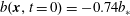 $b(\boldsymbol{x},t=0)=-0.74b_{\ast }$.

Figure 6. Approach to statistical equilibrium for 2-D free-slip simulations at  $Ra=6.4\times 10^{10}$. We show three initial buoyancy conditions
  $b(x,z,0)=b_{\star }\times (0,-0.74,-0.9)$. (a) Domain-averaged kinetic energy. (b) The Nusselt number
  $Nu(t)$. (c) The bottom buoyancy
  $\bar{b}(z=0)/b_{\star }$.
In figure 5 we used the cold initial buoyancy  $-0.74b_{\star }$ that is suggested by the long calculation in figure 4(c). But usually one must guess at the initial buoyancy which is closest to the ultimate bottom buoyancy. The three solutions shown in figure 6 indicate that the consequences of a guess that is too cold are not serious. The solution with initial buoyancy
  $b(x,z,0)=-0.9b_{\star }$ is too cold: the bottom buoyancy must increase to about
  $-0.75b_{\star }$ in the long-time state. Nonetheless, the Nusselt number of the too-cold solution in figure 6(b) equilibrates quickly. Moreover to estimate
  $Nu$ it is better to start too cold than too warm: the too-warm initial condition in figure 6, i.e.
  $b(x,z,0)=0$, has a large initial transient in the kinetic energy and
  $Nu(t)$ does not stabilize until about
  $t=0.2h^{2}/\unicode[STIX]{x1D705}$. The kinetic energy and bottom buoyancy in figure 6(a,c) require longer evolution than
  $Nu(t)$ in order to achieve their final values. Additionally, the transient period for the too-cold initial condition has a much weaker flow compared to the vigorous transient flow of the too-warm solution (see figure 6a); this reduces the computational effort required to reach statistical steady state.

Figure 7. A comparison of the ‘instantaneous Nusselt number’ time series for (a) the 2-D free-slip solution at  $Ra=6.4\times 10^{10}$ with initial condition
  $b(x,z,0)=0$ and (b) the 3-D free-slip solution at
  $Ra=6.4\times 10^{10}$ with initial condition
  $b(x,z,0)=-0.74b_{\star }$. In both cases
  $Pr=1$. Nusselt number
  $Nu(t)$ is defined via the volume average of
  $\unicode[STIX]{x1D705}|\unicode[STIX]{x1D735}b|^{2}$, i.e. the second term on the right-hand side of (4.3). The surface Nusselt number,
  $Nu_{s}(t)$, is defined via the surface average of
  $b_{s}$ times the flux
  $\unicode[STIX]{x1D705}b_{z}(x,h,t)$, i.e. the first term on the right-hand side of (4.3). Nusselt number
  $Nu_{F}(t)$ is defined as in (3.4) without the time average. The time series in (b) is from the solution shown in figures 1 and 2.
4.3 The surface Nusselt number $Nu_{s}$

The identity (3.8) provides an alternative means of diagnosing  $Nu$ by measuring the buoyancy flux
  $\unicode[STIX]{x1D705}b_{z}(x,y,h,t)$ through the top surface of the domain. We refer to this second Nusselt number as the ‘surface Nusselt number’, denoted
  $Nu_{s}(t)$. Multiplying the buoyancy equation (2.2) by
  $b$, and integrating over the volume of the domain, we obtain
 $$\begin{eqnarray}\frac{\text{d}}{\text{d}t}\int {\textstyle \frac{1}{2}}b^{2}\,\text{d}V=\int _{z=h}b_{s}\unicode[STIX]{x1D705}b_{z}\,\text{d}A-\unicode[STIX]{x1D705}\int |\unicode[STIX]{x1D735}b|^{2}\,\text{d}V.\end{eqnarray}$$
 This shows that the difference between  $Nu_{s}(t)$ and
  $Nu(t)$ – the two terms on the right-hand side of (4.3) – is related to temporal fluctuations in the domain-integrated buoyancy variance. The buoyancy power integral (3.8) is obtained by time-averaging (4.3).
Figure 7 shows that during the initial transient there are substantial differences between  $Nu(t)$ and
  $Nu_{s}(t)$. But after the transient subsides,
  $Nu(t)$ and
  $Nu_{s}(t)$ are almost equal, even without time-averaging. This coincidence is most striking in the 2-D solution shown figure 7(a). For the 3-D solution in figure 7(b),
  $Nu_{s}(t)$ closely follows
  $Nu(t)$, except for the small high-frequency variability evident in
  $Nu_{s}(t)$, but not in
  $Nu(t)$.
This close agreement between  $Nu(t)$ and
  $Nu_{s}(t)$ indicates that in statistical steady state the left-hand side of (4.3) is a small residual between the two much larger terms on the right-hand side. This indicates that the buoyancy boundary layer is strongly controlled by diffusion. Moreover, the source of the low-frequency temporal variability in
  $Nu(t)$ and
  $Nu_{s}(t)$ is the same in the 2-D and 3-D cases and results from large-scale, dominantly 2-D, interior eddies stirring the boundary layer. The high-frequency variability evident in the 3-D
  $Nu_{s}(t)$ likely results from the small-scale spanwise (
 $y$) boundary-layer variability evident in figure 1. Although the time series in figure 7(b) is from a 3-D solution, the spanwise components are weak:
 $$\begin{eqnarray}\frac{\langle v^{2}\rangle }{\langle u^{2}+v^{2}+w^{2}\rangle }\approx 0.11\quad \text{and}\quad \frac{\langle b_{y}^{2}\rangle }{\langle b_{x}^{2}+b_{y}^{2}+b_{z}^{2}\rangle }\approx 0.012.\end{eqnarray}$$
 Thus, despite the visual impression from figure 1, the solution is dominantly 2-D with weak spanwise perturbations. To obtain a robustly 3-D flow, it seems that  $Ra$ must be increased above
  $6.4\times 10^{10}$ in figure 1. This conclusion is supported by the numerical insensitivity of
  $Nu$ to both boundary condition and dimensionality evident in figure 5: the time-averaged Nusselt varies by less than a factor of two, from
  $25.5$ for no-slip 2-D to
  $43.9$ for free-slip 3-D. Moreover the viscous boundary condition has a larger quantitative effect on
  $Nu$ than does dimensionality: in figure 5 the 2-D free-slip solution has larger
  $Nu$ than that of the 3-D no-slip solution.
In the context of 2-D very viscous ( $Pr=\infty$) HC, Chiu-Webster et al. (Reference Chiu-Webster, Hinch and Lister2008) show that important structural features of the flow are independent of boundary condition. The result in figure 5 is numerical evidence that this insensitivity to the viscous boundary condition extends to 3-D HC with
  $Pr=1$.
Direct evaluation of  $\unicode[STIX]{x1D712}$ via definition (3.7) requires the volume integral of
  $|\unicode[STIX]{x1D735}b|^{2}$; this integrand is concentrated on small spatial scales. Thus in an experimental situation it is likely impossible to evaluate
  $\unicode[STIX]{x1D712}$ directly from (3.7). The identity (4.3) shows that
  $\unicode[STIX]{x1D712}$ can alternatively be estimated from a surface integral involving the vertical buoyancy flux through the non-uniform surface – this is the flux of entropy through the surface required to balance interior entropy production associated with molecular diffusion of heat. Figure 3(a) indicates that the surface entropy flux,
  $b_{s}F$, is a smooth, large-scale quantity. Thus
  $Nu_{s}$ is accessible to experimental measurement. Numerical solutions provide both
  $Nu$ and
  $Nu_{s}$ and one can use this information to test if the solution is in statistical steady state, e.g. as in figure 7.
4.4 The Nusselt number $Nu_{F}$ and its relation to $Nu$ and $Nu_{s}$


In § 4.1 we concluded that the time average of  $Nu(t)$ can be obtained with computations that are significantly shorter than the vertical diffusion time
  $h^{2}/\unicode[STIX]{x1D705}$. This conclusion probably extends to the alternative Nusselt numbers discussed in § 3: all these measures of buoyancy flux are designed to diagnose the thickness of the surface boundary layer and likely exhibit the rapid equilibration in figure 4(b). In support of this conclusion, figure 7(a) shows a time series of Rossby’s Nusselt number
  $Nu_{F}(t)$ in (3.4). Nusselt number
  $Nu_{F}(t)$ is in close agreement with
  $Nu(t)$ and
  $Nu_{s}(t)$. Moreover, the ratio
  $Nu_{F}(t)/Nu_{s}(t)$ fluctuates around 1.04 (not shown).
We were surprised by the close numerical agreement of  $Nu_{F}(t)$ with the other Nusselt numbers: a priori one anticipates that
  $Nu_{F}$ should differ from
  $Nu(t)$ and
  $Nu_{s}(t)$ by a non-dimensional multiplier. But why is this multiplier close to one? We can explain this coincidence using the formula for the effective diffusivity in (3.18). For the sinusoidal buoyancy profile
  $b_{s}(x)$ in (2.4), the diffusive solution is
 $$\begin{eqnarray}b_{diff}=\underbrace{b_{\star }\cos (kx)}_{b_{s}(x)}\,\frac{\cosh kz}{\cosh kh},\end{eqnarray}$$
and so the effective diffusivity in (3.18) is
 $$\begin{eqnarray}D=Nu\,\unicode[STIX]{x1D705}\frac{\tanh (kh)}{kh}.\end{eqnarray}$$
 On the other hand, from (3.12) and (3.14), the vertical flux is  $F\approx k^{2}hDb_{s}$; this result can be used to evaluate the numerator in
  $Nu_{F}$, and the denominator follows from (4.5):
 $$\begin{eqnarray}\displaystyle Nu_{F} & {\approx} & \displaystyle \frac{D}{\unicode[STIX]{x1D705}}\frac{kh}{\tanh (kh)}\end{eqnarray}$$
 $$\begin{eqnarray}\displaystyle & {\approx} & \displaystyle Nu,\end{eqnarray}$$
 where (4.6) was used in passing from (4.7) to (4.8). Note that this result relies on special properties of the sinusoidal  $b_{s}(x)$; for other surface buoyancy profiles,
  $Nu_{F}/Nu$ will not necessarily be close to one.
5 Conclusion
In § 3 we discussed four different Nusselt numbers used as indices of horizontal-convective heat transport. We advocate adoption of  $Nu=\unicode[STIX]{x1D712}/\unicode[STIX]{x1D712}_{diff}$ as the primary index of the strength of HC. This particular Nusselt number is based on
  $\unicode[STIX]{x1D712}=\unicode[STIX]{x1D705}\langle |\unicode[STIX]{x1D735}b|^{2}\rangle$, which, up to a constant multiplier, is the volume-averaged rate of Boussinesq entropy production. An advantage of
  $\unicode[STIX]{x1D712}/\unicode[STIX]{x1D712}_{diff}$ over alternative HC Nusselt numbers discussed in § 3 is that the Nusselt number of RBC can also be expressed as
  $\unicode[STIX]{x1D712}/\unicode[STIX]{x1D712}_{diff}$. Thus the thermodynamic interpretation in terms of entropy production provides a unified framework for both varieties of convection.
The surface Nusselt number,  $Nu_{s}$, of § 4.3 is the flux of entropy through the non-uniform surface; in statistically steady state the surface entropy flux balances interior production. In experimental situations it is easier to measure the surface integral of
  $b_{s}F$ required for
  $Nu_{s}$ than the volume integral of
  $|\unicode[STIX]{x1D735}b|^{2}$ demanded by
  $Nu$. Figure 7 shows that time series of
  $Nu(t)$ and
  $Nu_{s}(t)$ are almost equal. This coincidence indicates that the surface boundary layer is dominated by buoyancy diffusion, even at
  $Ra=6.4\times 10^{10}$ used in figure 7.
The power integral  $\overline{\boldsymbol{J}\boldsymbol{\cdot }\unicode[STIX]{x1D735}b_{s}}=-\unicode[STIX]{x1D712}$ provides a connection between
  $Nu$ and the horizontal buoyancy flux
  $\boldsymbol{J}$. Using this relation one can introduce the effective diffusivity
  $D$ in (3.17) and (3.18) such that
  $\boldsymbol{J}\approx -D\unicode[STIX]{x1D735}b_{s}$. This establishes a relation between entropy production and horizontal-convective buoyancy flux.
In § 4 we showed that  $Nu(t)$ equilibrates more rapidly than other average properties of HC, such as volume-averaged kinetic energy and bottom buoyancy. With a cold start, the long-term average of
  $Nu(t)$ can be estimated with integrations that are much shorter than a diffusive time scale (see figures 5 and 6b). These numerical results indicate that entropy production,
  $\unicode[STIX]{x1D712}$, is strongly concentrated in an upper boundary layer and that fast diffusion through this thin layer results in rapid equilibration of
  $Nu$ and
  $Nu_{s}$.
The thermodynamic interpretation of  $\unicode[STIX]{x1D712}$ explains why
  $\unicode[STIX]{x1D712}$ participates in so many identities and inequalities. Alternative Nusselt numbers, such as
  $Nu_{F}$ in (3.4), do not lead to an analytic framework that can be explored and exploited by variational methods. Thus bounds on the
  $Nu$–
$Nu$– $Ra$ relation of HC employ
  $\unicode[STIX]{x1D712}/\unicode[STIX]{x1D712}_{diff}$ (Siggers et al. Reference Siggers, Kerswell and Balmforth2004; Rocha et al. Reference Rocha, Bossy, Llewellyn Smith and Young2020). Nusselt definitions that use
  $|F|$ as a device to obtain a non-zero measure of the surface buoyancy flux are arbitrary to the extent that the mean of
  $F^{2}$, or indeed any other functional norm of
  $F$ or
  $J$, might be employed. These alternatives to entropy production do not have a link to the Boussinesq equations of motion and are not as useful as
  $Nu=\unicode[STIX]{x1D712}/\unicode[STIX]{x1D712}_{diff}$.
Acknowledgements
We thank T. Sohail for help with figure 1 and B. Gallet and T. Bossy for discussion of horizontal convection. We thank the three referees for comments that greatly improved this paper. Computer resources were provided by the Australian National Computational Infrastructure at ANU, which is supported by the Commonwealth of Australia. W.R.Y. was supported by National Science Foundation Award OCE-1657041.
Declaration of interests
The authors report no conflict of interest.


 Open access