


1. Introduction
The mixing of scalars and their release to a surrounding fluid are of overwhelming importance for a plethora of industrial and environmental flows. Examples are the release and propagation of airborne molecules in free or enclosed spaces, atmospheric or oceanic thermal motions and combustion in closed chambers. The simplest paradigm for turbulent mixing is when a substance is a scalar characterized only by its concentration that does not influence the flow (Shraiman & Siggia Reference Shraiman and Siggia2000; Warhaft Reference Warhaft2000). Turbulent mixing is a process that naturally occurs when regions at different scalar concentrations interact (Eswaran & Pope Reference Eswaran and Pope1988; Overholt & Pope Reference Overholt and Pope1996). As a consequence, mixing is inherently associated with statistically inhomogeneous anisotropic flows (Craske, Debugne & van Reeuwijk Reference Craske, Debugne and van Reeuwijk2015). It can be viewed as being composed of two elementary processes: turbulent stirring and diffusion (Holzer & Siggia Reference Holzer and Siggia1994; Pumir Reference Pumir1994; Dimotakis Reference Dimotakis2005). The former is a result of the motion induced by turbulence while the latter is a result of the scalar concentration gradients. From a local perspective, these two processes have opposite effects on the scalar concentration gradients and thus contrast each other. Molecular diffusion causes the homogenization of the scalar concentration, thus eroding the concentration gradients and the effectiveness of the diffusion itself. On the contrary, the scalar stirring induced by the fluctuating velocity field sustains the scalar concentration gradients by distorting and pushing toward each other the scalar iso-concentration surfaces (Sreenivasan Reference Sreenivasan2019). When the free-surface boundary of a passive scalar flow is considered, the velocity stirring of the scalar field is commonly distinguished in large-scale engulfment and small-scale nibbling (Mathew & Basu Reference Mathew and Basu2002; Westerweel et al. Reference Westerweel, Fukushima, Pedersen and Hunt2005, Reference Westerweel, Fukushima, Pedersen and Hunt2009; Watanabe et al. Reference Watanabe, Sakai, Nagata, Ito and Hayase2015; Borrell & Jiménez Reference Borrell and Jiménez2016; Jahanbakhshi & Madnia Reference Jahanbakhshi and Madnia2016) and the concentration flux across the so-called scalar interface is of overwhelming importance for applications and needs to be understood (Holzner & Lüthi Reference Holzner and Lüthi2011; da Silva et al. Reference da Silva, Hunt, Eames and Westerweel2014).
The process of stirring of scalar iso-concentration surfaces is initiated with the large-scale coherent structures of turbulence by engulfment of fluid at different scalar concentrations. The scalar entrapped by the large-scale motions is then further processed by nibbling mechanisms at smaller and smaller scales produced by the turbulent cascade where, finally, molecular diffusion is rapid enough to complete the turbulent entrainment and mixing. It is then evident that turbulent mixing is a spatially evolving cascade process involving the full spectrum of scales (Sreenivasan Reference Sreenivasan1996; Schumacher & Sreenivasan Reference Schumacher and Sreenivasan2005; Schumacher, Sreenivasan & Yeung Reference Schumacher, Sreenivasan and Yeung2005; Cimarelli et al. Reference Cimarelli, Cocconi, Frohnapfel and De Angelis2015, Reference Cimarelli, Mollicone, van Reeuwijk and De Angelis2021) and different flow regions. Hence, it is legitimate to study the turbulent mixing from both the large- and small-scale perspective. The first stage of the process, at the large scale of motion, is highly influenced by the flow configuration, large scales being the result of the flow instability. On the other hand, the last stage of turbulent mixing, at small scales, is characterized by a larger degree of universality.
This multi-scale nature of turbulent mixing calls for a multi-scale analysis of the process as demonstrated by a number of recent works. As an example, Philip et al. (Reference Philip, Meneveau, de Silva and Marusic2014) and Mistry et al. (Reference Mistry, Philip, Dawson and Marusic2016) studied the entrainment process by analysing particle image velocimetry data of a turbulent boundary layer and of an axisymmetric jet, respectively, decomposed in a hierarchy of scales by means of a spatial filtering operation. This approach provided evidence that large-scale transport determines the overall rate of entrainment but that the actual entrainment occurs physically at small diffusive scales along the interface. This result supports the interpretation of viscous nibbling as a small-scale process and inviscid engulfment as a large-scale one. More recently, in Cimarelli et al. (Reference Cimarelli, Cocconi, Frohnapfel and De Angelis2015) the spectral balance equation of enstrophy was used to study the multi-scale properties of entrainment in decaying shear-less turbulence. A strongly anisotropic cascade process is revealed to occur at the turbulent front consisting of a transfer of enstrophy towards smaller and smaller normal-to-the-interface scales while retaining very large parallel-to-the-interface scales. In agreement with this picture, the scale-by-scale analysis of the turbulent kinetic energy reported in Watanabe, da Silva & Nagata (Reference Watanabe, da Silva and Nagata2020) highlights the simultaneous presence of forward cascade processes for the normal-to-the-interface scales and reverse cascade processes for the parallel-to-the-interface scales. These multi-scale spatially evolving cascade mechanisms have been finally rigorously explained in Cimarelli et al. (Reference Cimarelli, Mollicone, van Reeuwijk and De Angelis2021) by means of the theoretical framework provided by the generalized Kolmogorov equation.
One of the main limitations in the understanding of turbulence entrainment and mixing is the lack of dynamical information of the process, i.e. the cause and the effect of the elementary processes composing the flow system. Most of the studies mentioned above deal with the analysis of flow realization snapshots, thus losing possible information about the dynamic causality of the phenomena that naturally occur over time. In this context, it would be important to assess the previously shown multi-scale mechanisms of turbulent entrainment and mixing from a dynamic point of view. In the present work, we address this issue by analysing the evolution of the process under the separate action of large and small velocity scales. To this aim, numerical experiments are performed where the velocity coupling of the passive scalar equation with the Navier–Stokes equations is modified to alternatively suppress the role of large and small velocity scales in the process of scalar mixing. Hence, this approach allows us to clearly assess their contribution from a dynamical point of view. To the authors’ knowledge this is the first attempt to address the dynamic causality of large and small velocity scales in turbulent mixing and entrainment of a scalar.
The paper is organized as follows. The numerical settings and the main flow features of the temporal planar jet are shown in § 2. Some heuristic arguments in support of the relevance of the different scales of turbulence in the scalar mixing process are reported in § 3. The numerical experiments are described in § 4 and their results are presented in § 5. In § 6, some insights into the essential processes at the basis of turbulent entrainment and mixing are envisaged. Finally, the work is closed by concluding remarks in § 7.
2. Temporal jet
2.1. Numerical settings
The selected base flow for the numerical experiments on turbulent entrainment and mixing is a turbulent planar temporal jet (da Silva & Pereira Reference da Silva and Pereira2008; van Reeuwijk & Holzner Reference van Reeuwijk and Holzner2014; Cimarelli et al. Reference Cimarelli, Mollicone, van Reeuwijk and De Angelis2021). This type of flow represents a paradigm for free shear flows by reproducing essential flow features such as an inhomogeneous mean shear, a turbulent/non-turbulent interface region and a simultaneous presence of two interacting well-separated ranges of scales: the large-scale motions reminiscent of the Kelvin–Helmholtz instability and the small-scale fluctuations of the developed turbulent motion. The main advantage of this type of flow with respect to other paradigms, e.g. spatially developing jets, mixing layers and wakes (Stanley, Sarkar & Mellado González Reference Stanley, Sarkar and Mellado González2002), is the two-dimensional statistical spatial homogeneity. Indeed, the flow develops in time rather than in the streamwise direction thus gaining a statistical spatial homogeneity and losing the statistical homogeneity in time.
The flow is governed by the Navier–Stokes equations coupled with the evolution of a passive scalar:
 \begin{equation} \left.\begin{gathered}
\frac{\partial u_i}{\partial x_i} = 0, \\[-4pt] \frac{\partial
u_i}{\partial t} + \frac{\partial u_i u_j}{\partial x_j}
={-}\frac{\partial p}{\partial x_i} + \frac{1}{Re}
\frac{\partial^2 u_i}{\partial x_j \partial x_j}, \\ [-4pt]
\frac{\partial \theta}{\partial t} + \frac{\partial \theta
u_j}{\partial x_j} = \frac{1}{Re Sc}\frac{\partial^2
\theta}{\partial x_j \partial x_j}.
\end{gathered}\right\} \end{equation}
\begin{equation} \left.\begin{gathered}
\frac{\partial u_i}{\partial x_i} = 0, \\[-4pt] \frac{\partial
u_i}{\partial t} + \frac{\partial u_i u_j}{\partial x_j}
={-}\frac{\partial p}{\partial x_i} + \frac{1}{Re}
\frac{\partial^2 u_i}{\partial x_j \partial x_j}, \\ [-4pt]
\frac{\partial \theta}{\partial t} + \frac{\partial \theta
u_j}{\partial x_j} = \frac{1}{Re Sc}\frac{\partial^2
\theta}{\partial x_j \partial x_j}.
\end{gathered}\right\} \end{equation}
Equations (2.1) are written in a dimensionless form by using the initial jet width  $H$ for the length scales, the initial jet velocity $U_0$ for the velocity scales and the initial jet scalar concentration $C_0$ for the scalar scales. When not specifically stated, all the results of the present work are reported dimensionless by using $H$,
$H$,  $U_0$ and $C_0$ as reference scales. Here $Re = U_0 H / \nu$ is the Reynolds number, where $\nu$ is the kinematic viscosity, while $Sc = \nu / \alpha$ is the Schmidt number, where $\alpha$ is the diffusivity of the scalar. In (2.1), index $i=1,2,3$ corresponds to the streamwise, spanwise and cross-flow $(u,v,w)$ velocities and $(x,y,z)$ directions. Equations (2.1) are solved using the open-source code Incompact3d (Laizet & Lamballais Reference Laizet and Lamballais2009). The spatial discretization is based on a high-order compact finite-difference scheme, sixth-order accurate, and the time integration is performed using a third-order Runge–Kutta scheme. Periodic boundary conditions are applied in all directions.
The initial condition is a fluid layer that is quiescent and characterized by a null concentration of the scalar except for a thin region  $-H/2< z< H/2$ where the streamwise velocity and the scalar are non-zero and homogeneously distributed in the streamwise and spanwise directions:
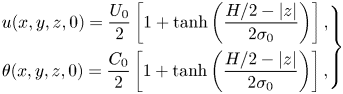 \begin{equation} \left.\begin{gathered}
u (x,y,z,0) = \frac{U_0}{2} \left [ 1 + \tanh \left (
\frac{H/2 -|z|}{2 \sigma_0} \right ) \right ] ,\\ \theta
(x,y,z,0) = \frac{C_0}{2} \left [ 1 + \tanh \left (
\frac{H/2 -|z|}{2 \sigma_0} \right ) \right ], \end{gathered}\right\}
\end{equation}
\begin{equation} \left.\begin{gathered}
u (x,y,z,0) = \frac{U_0}{2} \left [ 1 + \tanh \left (
\frac{H/2 -|z|}{2 \sigma_0} \right ) \right ] ,\\ \theta
(x,y,z,0) = \frac{C_0}{2} \left [ 1 + \tanh \left (
\frac{H/2 -|z|}{2 \sigma_0} \right ) \right ], \end{gathered}\right\}
\end{equation}
where  $\sigma _0 = H / 35$ is the initial momentum thickness. In order to facilitate a rapid transition to turbulence, a perturbation is superimposed to the initial condition of all three components of the velocity field consisting of a uniform random noise whose amplitude is $0.01 U_0$.
The simulations have been performed for  $Re = 3000$ and $Sc = 1$. The numerical domain is a cuboid of size $36H \times 36H \times 24H$ discretized with $900 \times 900 \times 600$ equally spaced points, thus leading to the same resolution in all three spatial directions. The worst condition for the resolution is reached at the centreline during the initial turbulent transition for $t = 20$ where $\Delta x / \eta _{cl} \approx 4.5$ with $\eta _{cl}$ the centreline value of the Kolmogorov scale. As shown in the following, in the self-similar decay of the flow, the Kolmogorov scale increases from this minimum both in time $\eta _{cl} \propto \sqrt {t}$ and with cross-flow position, thus highlighting that the spatial resolution employed is appropriate (see also the Appendix where a validation of the numerical solution is reported). Finally, a constant time step $\Delta t = 0.01$ has been used leading to a Courant–Friedrichs–Lewy (CFL) number that on average is $\textrm {CFL} \approx 0.3$.
Averages, hereafter denoted as  $\langle \cdot \rangle$, have been computed by taking advantage of the statistical properties of the flow, i.e. spatial homogeneity in the streamwise and spanwise directions and symmetry in the cross-flow direction, and by using an ensemble of two independent flow realizations obtained using different random perturbations in the initial conditions. The customary Reynolds decomposition of the flow in a mean and fluctuating field is adopted:
 $$\begin{gather} \boldsymbol{u} = \boldsymbol{U} + \boldsymbol{\upsilon}, \end{gather}$$
 $$\begin{gather}\theta = \varTheta + \vartheta, \end{gather}$$
where  $\boldsymbol {U} = \langle \boldsymbol {u} \rangle$ and $\varTheta = \langle \theta \rangle$ are the average fields and $\boldsymbol {\upsilon }$ and $\vartheta$ are the fluctuating ones.
2.2. Flow features and self-similarity
The evolution of the flow is shown in figure 1 by means of iso-contours of the scalar field at different time instants. From the initial condition, the flow field exhibits first Kelvin–Helmholtz-like instabilities and then transitional mechanisms giving rise to turbulent fluctuations. As shown in figure 2(a), these production mechanisms of turbulent fluctuations exceed the dissipative ones giving rise to an increase of the turbulent kinetic energy and of the scalar variance content up to  $t \approx 15$ and $t \approx 20$ where the maxima of $\langle \vartheta \vartheta \rangle _{cl} (t) = \langle \vartheta \vartheta \rangle (z=0,t)$ and $k_{cl} (t) = \langle \upsilon _i \upsilon _i \rangle (z=0,t)/ 2$ are reached, respectively. Hence, for $t > 20$, turbulence starts to decay. As shown by the instantaneous behaviour of the scalar field in figure 1, the flow, while decaying, performs entrainment and mixing producing increasingly larger scales of motion and increasing its width. Note that also at the latest stages of the decay, the large-scale structures of the main flow instability are still visible.
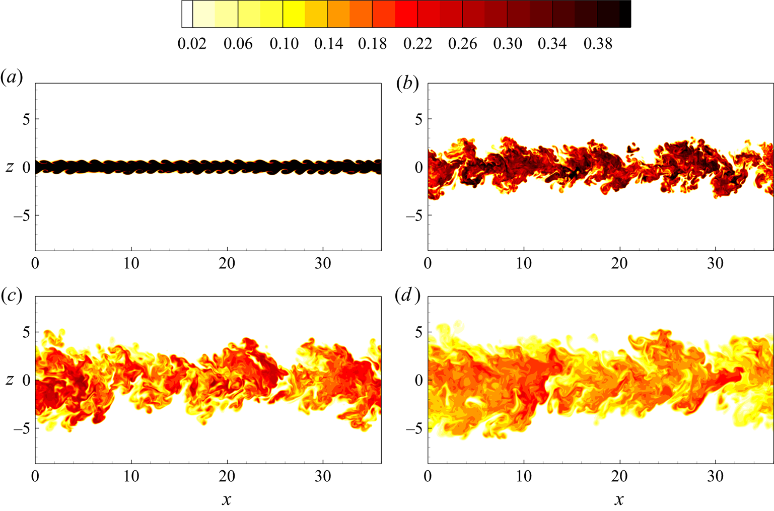
Figure 1. Direct numerical simulation of a turbulent temporal jet. Iso-contours of the scalar field  $\theta = [0,0.4]$ for $t=$ (a) 10, (b) 35, (c) 70 and (d) 105.
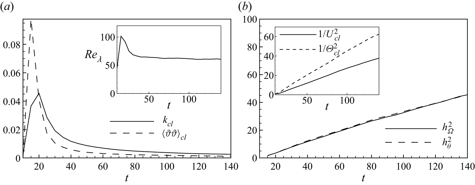
Figure 2. (a) Temporal evolution of the centreline turbulent kinetic energy  $k_{cl}$ and of the centreline scalar variance $\langle \vartheta \vartheta \rangle _{cl}$. The behaviour of the Taylor Reynolds number is shown in the inset. (b) Self-similar behaviour of the jet half-widths, $h_\varOmega$ and $h_\theta$, and of the mean centreline velocity and scalar concentration, $U_{cl}$ and $\varTheta _{cl}$ (inset).
The decay of the flow is characterized by a self-similar behaviour. The only relevant parameters in the self-similar regime are the volume flux  $Q_0 \equiv \int U \,\textrm {d}z$, the cross-sectional scalar content $C_0 \equiv \int \varTheta \,\textrm {d} z$ and the time $t$. The former two are invariant for this flow type. The conserved quantities, $Q_0=\text {const.}$ and $C_0=\text {const.}$, can be easily derived from the cross-stream integration of the mean streamwise momentum equation and of the mean scalar equation, respectively. These three relevant parameters immediately imply that the self-similar decay is characterized by an increase of the length scales as $\sqrt {Q_0 t}$ and by a decrease of the velocity and scalar scales as $\sqrt {Q_0 / t}$ and $C_0 /\sqrt {Q_0t}$, respectively. In figure 2(b), we show the behaviour of the mean centreline velocity and scalar concentration, $U_{cl} (t) = U (z=0,t)$ and $\varTheta _{cl} (t) = \varTheta (z=0,t)$, and of the jet half-widths $h_\varOmega$ and $h_\theta$, defined as the centreline distance where the mean enstrophy and scalar profiles reduce to 2 % their centreline value. From the plot it is clear that the flow has reached a dynamic equilibrium for $t> 30$ when all the observables start to follow a self-similar behaviour. Note that the scalar and enstrophy interfaces measured by means of $h_\varOmega$ and $h_\theta$ almost collapse. In accordance with these scaling of velocities and lengths, the self-similar regime is characterized by a constant Taylor Reynolds number, $Re_\lambda = \sqrt {2 k_{cl}/3} \lambda _{cl} / \nu = 60$, where $\lambda _{cl} = \sqrt {10 \nu k_{cl} / \epsilon _{cl}}$ is the centreline value of the Taylor microscale and $\epsilon _{cl}$ the centreline turbulent dissipation (see the inset of figure 2a).
3. A heuristic view of entrainment and mixing
The evolution of scalar fields is governed by inertial and diffusive transport phenomena. The mixing and entrainment properties of the scalar are, hence, the result of complex dynamical interactions between these two processes. Indeed, scalar entrainment is directly accomplished by diffusive mechanisms only, but, from a dynamical point of view, their strength significantly depends on the properties of the inertial scalar fluxes especially in turbulent flows. It is then reasonable to use information from both the inertial and diffusive phenomena to argue about the rate of scalar entrainment and mixing. Based on heuristic arguments, we try here give an estimate of these two processes by considering general scale-dependent properties of the flow motion. Indeed, in the case of Schmidt number close to unity, both mixing due to turbulence convection and scalar diffusion occur at similar length and time scales. These predictions are then used to produce alternative scalings for the rate of scalar entrainment and mixing.
The diffusive flux across iso-concentration surfaces can be generally estimated as
 \begin{equation} \phi_\alpha \equiv \alpha \frac{\mathcal{C}}{\ell} S_\ell, \end{equation}
where  $\mathcal {C}$ is a characteristic scalar concentration and $S_\ell$ is the area of the scalar interface indirectly induced by a turbulent motion with cutoff scale $\ell$ (Catrakis, Aguirre & Ruiz-Plancarte Reference Catrakis, Aguirre and Ruiz-Plancarte2002). On the other hand, the turbulent scalar flux across iso-concentration surfaces is directly determined by the convective action of the turbulent field and can be estimated as
 \begin{equation} \phi_{u} \equiv \mathcal{C} u_\ell S_\ell, \end{equation}
where  $u_\ell$ is the characteristic velocity difference of a turbulent motion with cutoff scale $\ell$. Let us recall that this reasoning applies for flows of unity Schmidt number where the velocity and scalar cutoff length scales are similar. Equations (3.1) and (3.2) highlight that the essential role of turbulent motion is to influence the convoluted scalar surfaces by prescribing the interface area $S_\ell$ and its fluctuation $u_\ell$, thus influencing both the diffusive and inertial scalar fluxes.
Based on the assumption that iso-surfaces in turbulence are fractal-like, it is possible to derive a useful relation for estimating the area of complex turbulence surfaces:
 \begin{equation} S_\ell =S_0 \left ( \frac{\ell}{L} \right )^{2-D}, \end{equation}
where  $S_0$ and $L$ are some characteristic area and length and $D$ is the fractal dimension of the surface. In this context, a fundamental result has been obtained by Sreenivasan, Ramshankar & Meneveau (Reference Sreenivasan, Ramshankar and Meneveau1989). Indeed, by assuming that all fluxes across iso-surfaces are independent of Reynolds number, Sreenivasan et al. (Reference Sreenivasan, Ramshankar and Meneveau1989) found that an estimate of the fractal dimension of turbulent interfaces is $D= 7/3$ in good agreement with experimental results. By inserting the estimate of the surface area (3.3) in the models for the diffusive and inertial scalar fluxes (3.1) and (3.2), we obtain the following relations:
 $$\begin{gather} \phi_\alpha = \alpha \frac{\mathcal{C}}{\ell} S_0 \left ( \frac{\ell}{L} \right )^{2-D}, \end{gather}$$
 $$\begin{gather}\phi_{u} = \mathcal{C} u_\ell S_0 \left ( \frac{\ell}{L} \right )^{2-D}. \end{gather}$$
It is useful now to introduce the relative speed of a scalar iso-concentration surface:
 \begin{equation} V_\theta = V_b - V_e, \end{equation}
where  $V_b$ is the boundary entrainment rate and $V_e$ is the entrainment velocity (da Silva et al. Reference da Silva, Hunt, Eames and Westerweel2014). By considering this entrainment parametrization, the scalar concentration flux can be globally estimated as
 \begin{equation} \phi = S_0 V_\theta \mathcal{C} . \end{equation}
It is now relevant to determine a scaling of  $V_\theta$ by using information from the inertial and diffusive fluxes. By equating this expression with the estimates (3.4) and (3.5), we can define two alternative scalings of the entrainment velocity:
 $$\begin{gather} V_\theta^\alpha = \frac{\alpha}{\ell} \left ( \frac{\ell}{L} \right )^{2-D}, \end{gather}$$
 $$\begin{gather}V_\theta^{u} = u_\ell \left ( \frac{\ell}{L} \right )^{2-D} . \end{gather}$$
Interestingly, these two relations do not depend on the characteristic scalar concentration, thus suggesting the relevance of studying the effects of the structure of the velocity field on the mixing properties of scalar fields as is done in the following sections.
4. Numerical experiments
As shown in the previous analysis, all the scales of the turbulent motion contribute to the wrinkling of the scalar interface; however, of general relevance is the understanding of the separated role played by the large (engulfment) and small (nibbling) scales. Indeed, it is reasonable to argue that the large-scale field is responsible for large-scale events of scalar transport and, hence, of deformation and stretching of the scalar interface. These large-scale phenomena are in general a result of motions related to the flow instability, such as the Kelvin–Helmholtz instability for the case of temporal jets. On the other hand, the small-scale motion is expected to be more universal at least for high Reynolds numbers. It is again reasonable to argue that small turbulent scales produce a less convoluted scalar interface but composed of smaller and smaller ripples.
It is then relevant to establish how the diffusive and convective laws of the scalar interface (3.4) and (3.5) change under the separate deformation action of large- and small-scale turbulent fluctuations. In the present work, we aim at dynamically establishing the above mentioned scale dependency of turbulent mixing and entrainment by performing numerical experiments where the scalar field is separately driven by large- and small-scale motions. First, a filtering operator is defined and applied to the velocity field:
 \begin{equation} \bar{\boldsymbol{u}} = \int G (\boldsymbol{x},\boldsymbol{\xi}) \boldsymbol{u} (\boldsymbol{\xi}) \,\textrm{d} \boldsymbol{\xi} ,\end{equation}
where
 \begin{equation} \int G (\boldsymbol{x},\boldsymbol{\xi}) \,\textrm{d} \boldsymbol{\xi} = 1 \end{equation}
and  $G$ is the kernel of a generic filter in space. The filtering formalism allows us to decompose the turbulent motion in the space of scales as
 \begin{equation} \boldsymbol{u} = \bar{\boldsymbol{u}} + \boldsymbol{u}' . \end{equation}
This decomposition of the velocity field is used to simulate the different dynamics of two independent scalar fields,  $\tilde {\theta }$ and $\theta ''$, separately driven by the large and small scales of the turbulence motion, respectively. The system of equations solved is
 \begin{equation} \left.\begin{gathered} \frac{\partial u_i}{\partial x_i} = 0
,\\ \frac{\partial u_i}{\partial t} + \frac{\partial u_i
u_j}{\partial x_j} ={-}\frac{\partial p}{\partial x_i} +
\frac{1}{Re} \frac{\partial^2 u_i}{\partial x_j \partial
x_j},\\ \frac{\partial \tilde{\theta}}{\partial t} +
\frac{\partial \tilde{\theta} \bar{u}_j}{\partial x_j} =
\frac{1}{Re Sc}\frac{\partial^2 \tilde{\theta}}{\partial
x_j \partial x_j},\\ \frac{\partial \theta''}{\partial t} +
\frac{\partial \theta'' u_j'}{\partial x_j} +
\frac{\partial \theta'' U_j}{\partial x_j} = \frac{1}{Re
Sc}\frac{\partial^2 \theta''}{\partial x_j \partial x_j},
\end{gathered}\right\}
\end{equation}
\begin{equation} \left.\begin{gathered} \frac{\partial u_i}{\partial x_i} = 0
,\\ \frac{\partial u_i}{\partial t} + \frac{\partial u_i
u_j}{\partial x_j} ={-}\frac{\partial p}{\partial x_i} +
\frac{1}{Re} \frac{\partial^2 u_i}{\partial x_j \partial
x_j},\\ \frac{\partial \tilde{\theta}}{\partial t} +
\frac{\partial \tilde{\theta} \bar{u}_j}{\partial x_j} =
\frac{1}{Re Sc}\frac{\partial^2 \tilde{\theta}}{\partial
x_j \partial x_j},\\ \frac{\partial \theta''}{\partial t} +
\frac{\partial \theta'' u_j'}{\partial x_j} +
\frac{\partial \theta'' U_j}{\partial x_j} = \frac{1}{Re
Sc}\frac{\partial^2 \theta''}{\partial x_j \partial x_j},
\end{gathered}\right\}
\end{equation}
thus highlighting that the evolution of the scalar field  $\tilde {\theta }$ is driven by a flow motion composed of large-scale fluctuations, $\tilde {\theta }= \tilde {\theta }[\bar {\boldsymbol {u}}]$. On the contrary, the scalar field $\theta ''$ evolves under the action of a flow motion composed of small-scale fluctuations, $\theta ''=\theta ''[\boldsymbol {U} + \boldsymbol {u}']$. As can be seen, for the scalar field $\theta ''$ the action of the mean flow has been explicitly added since $\langle \boldsymbol {u}' \rangle = 0$, while, for the scalar field $\tilde {\theta }$, the mean is implicitly included because $\langle \bar {\boldsymbol {u}} \rangle = \boldsymbol {U}$. It is important to notice that the filtering operation is applied for the sole decomposition of the velocity field in large and small scales that separately drive the evolution of the scalar fields $\tilde {\theta }$ and $\theta ''$, respectively. Hence, the two scalar fields $\tilde {\theta }$ and $\theta ''$ are the result of a different dynamical evolution imposed by the separate action of large- and small-scale motions and should not be confused with the filtering decomposition of the scalar field itself, i.e. $\theta \neq \tilde {\theta } + \theta ''$.
The initial conditions are taken from the unfiltered solution at  $t = 40$ thus allowing us to study the different evolution of $\tilde {\theta }$ and $\theta ''$ in the fully turbulent self-similar conditions of the flow. A two-dimensional Gaussian filter is employed in the two homogeneous directions, with characteristic length $\varDelta = 2.2 \lambda _{cl}$. Hence, the filter length increases during the flow decay as $\sqrt {t}$ by following the behaviour of the Taylor microscale $\lambda _{cl}$. By analysing other values of filter lengths, we found that the selected value $\varDelta = 2.2 \lambda _{cl}$ allows us to nicely split the large-scale motions typical of the main instability of the flow from the more homogeneous and isotropic small-scale turbulent field (da Silva, Lopes & Raman Reference da Silva, Lopes and Raman2015).
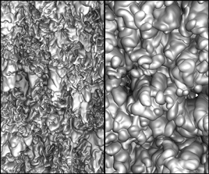
As shown in figure 3, the large-scale spanwise rolls reminiscent of the Kelvin–Helmholtz instability are carried by the large-scale field  $\bar {\boldsymbol {u}}$. Superimposed to this large-scale motion, very anisotropic turbulent fluctuations are also observed in the field $\bar {\boldsymbol {u}}$. On the contrary, no signature of large-scale spanwise rolls is found in the small-scale field $\boldsymbol {u}'$. This scenario is confirmed by the streamwise velocity spectra $E_k(k_x)$ evaluated at the jet interface $z=h_\theta$ and shown in figure 4(a). Indeed, the large-scale field $\bar {\boldsymbol {u}}$ is found to capture the large-scale spectral behaviour including the peak at small wavenumbers, while the small-scale field $\boldsymbol {u}'$ reproduces the small-scale spectral behaviour. In particular, the crossover scale between the two fields is found to take place well within the inertial range where the turbulent spectrum follows the classic $k^{-5/3}$ power law. Hence, the more homogeneous and isotropic small-scale fluctuations of the flow find their support in the field $\boldsymbol {u}'$.
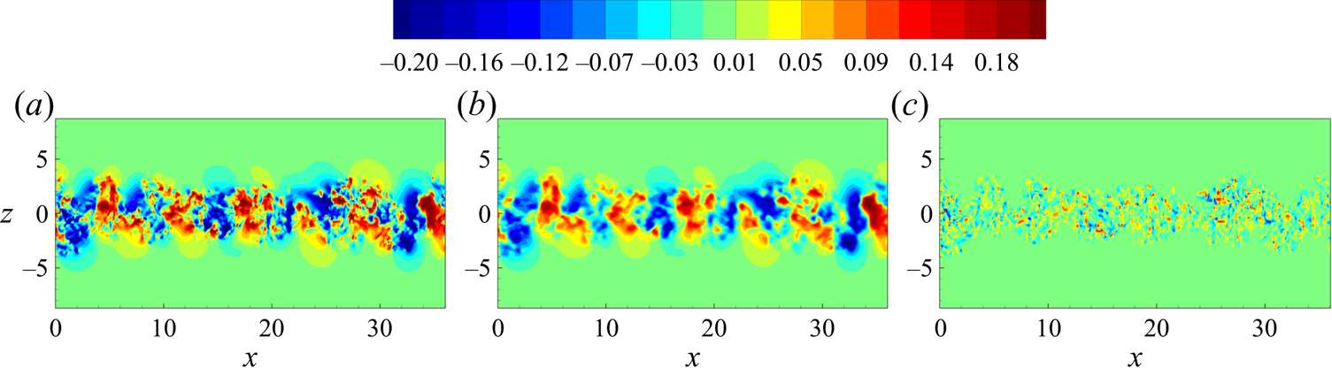
Figure 3. Iso-contours of the instantaneous cross-flow velocity,  $[-0.2,0.2]$, for $t=40$. The unfiltered field $\upsilon _3$ (a) is compared with the large- and small-scale fields, $\bar {\upsilon }_3$ (b) and $\upsilon _3'$ (c), respectively.
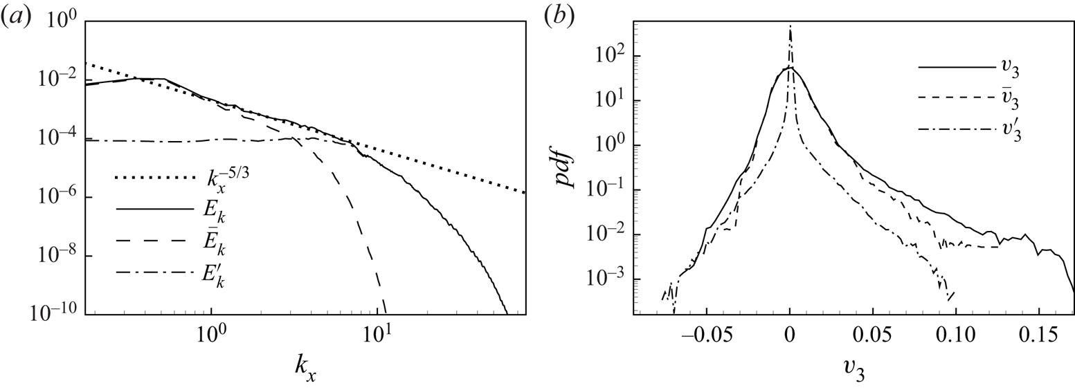
Figure 4. (a) Streamwise energy spectrum evaluated at the jet interface  $z=h_\theta$ for $t=40$. The unfiltered behaviour $E_{k}(k_x)$ is compared with the large- and small-scale velocity decomposition $\bar {E}_{k}$ and $E_{k}'$, respectively. (b) Probability density function of the cross-flow velocity component $\upsilon _3$ evaluated at the jet interface $z=h_\theta$ for $t=40$. The unfiltered behaviour $pdf(\upsilon _3)$ is compared with the large- and small-scale velocity decomposition $pdf(\bar {\upsilon }_3)$ and $pdf(\upsilon _3')$, respectively.
To better characterize the large- and small-scale fields, the probability density function of the velocity decomposition evaluated at the jet interface is shown in figure 4(b). The positively skewed distribution of the cross-flow velocity fluctuations at the interface is found to be almost entirely carried by the large-scale field  $\bar {\boldsymbol {u}}$. On the contrary, the small-scale field $\boldsymbol {u}'$ exhibits an almost symmetric distribution with a highly intermittent character. All these features are at the basis of the significantly different entrainment and mixing properties of the scalar field experiments that are discussed in the following section.
In closing this section, let us point out that other types of filter kernels, including also the filtering in the cross-flow direction, have been considered. The detailed study of the effects of the filter type, of the filter lengths and of the initial conditions on the evolution of the scalar fields described by the system of (4.4) is reported in Boga (Reference Boga2020). For the purpose of the present work, no physically relevant differences have been observed. In the same work, different filter lengths for the scalar fields  $\tilde {\theta }$ and $\theta ''$ have also been considered to enforce a separation of scales that due to the relatively low Reynolds number considered is otherwise limited. Again, no physically relevant phenomena are observed.
5. Results
We start by considering the scalar field evolution under the separate action of the large- and small-scale velocity fields. As shown in figure 5, the evolution of the scalar field  $\tilde {\theta }$ roughly resembles that of the unfiltered case $\theta$ in terms of both large-scale pattern and spreading of the jet. Indeed, the main difference between the two fields is given by the reduced amount of mixing, i.e. large-scale engulfment events are present but not combined with small-scale nibbling. As a result, at the final stages of the evolution for $t=140$, the region occupied by the scalar field $\tilde {\theta }$ is almost the same as that for $\theta$ but with the difference that unmixed flow regions of low-concentration levels are present within it. A completely different scenario appears for the scalar field $\theta ''$. In this case the large-scale pattern is completely different with respect to that of $\theta$, with large-scale engulfment events being completely suppressed. The low-concentration regions initially present within the jet for $t=50$ are absorbed during the evolution by the small-scale nibbling and diffusion, thus leading to a significantly more mixed turbulent jet at the final stage of the evolution for $t=140$. The completely different evolution of the two scalar fields $\tilde {\theta }$ and $\theta ''$ is also found to produce very distinct scalar-interface topologies for $t = 140$. A less convoluted interface with small-scale wrinkling is produced by the scalar field $\theta ''$ in contrast to a highly convoluted surface with almost absent small-scale wrinkling for the scalar field $\tilde {\theta }$.

Figure 5. Temporal evolution of the scalar fields. Iso-contours  $[0,0.4]$ of the scalar $\theta$ driven by the unfiltered velocity field (a–c), of the scalar $\tilde {\theta }$ driven by the large-scale velocity field (d–f) and of the scalar $\theta ''$ driven by the small-scale velocity field (g–i). Times $t =50$ (a,d,g), $t =95$ (b,e,h) and $t =140$ (c,f,i).
We analyse now the evolution of the three scalar fields  $\theta$, $\tilde {\theta }$ and $\theta ''$ from a statistical point of view. As shown in figure 6, the small-scale-driven scalar field $\theta ''$ shows a slower decay of the mean centreline scalar concentration together with a more rapid decay of its variance. On the contrary, the large-scale-driven scalar field $\tilde {\theta }$ shows a behaviour that more closely matches that of the unfiltered field in terms of mean scalar concentration decay, i.e. only a slightly slower decay is observed (see figure 6a). This matching of the unfiltered behaviour is, however, not observed when considering the scalar concentration variance. As shown in figure 6(b), a significantly slower decay of the scalar fluctuations is indeed observed.
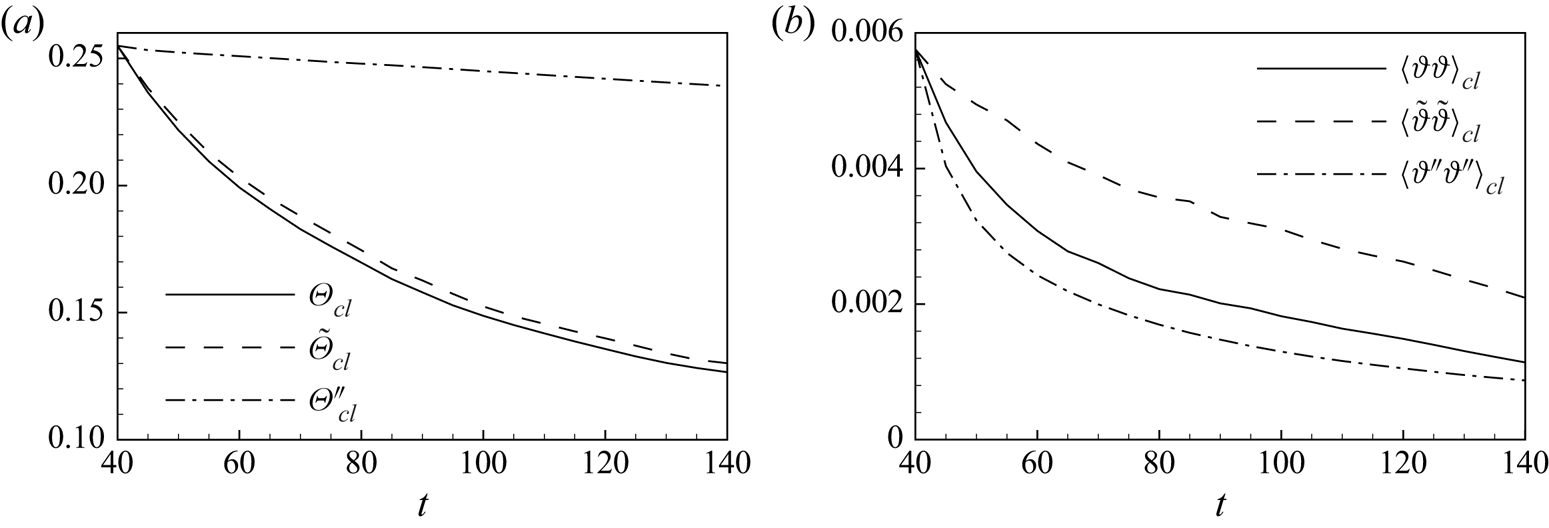
Figure 6. Temporal evolution of the centreline scalar mean (a) and variance (b) for the scalar fields  $\varTheta _{cl}$ and $\langle \vartheta \vartheta \rangle _{cl}$ (solid line), $\tilde {\varTheta }_{cl}$ and $\langle \tilde {\vartheta }\tilde {\vartheta } \rangle _{cl}$ (dashed line) and $\varTheta _{cl}''$ and $\langle \vartheta '' \vartheta '' \rangle _{cl}$ (dashed-dotted line).
The origin of these behaviours can be studied by considering the scalar variance budgets for  $\theta$, $\tilde {\theta }$ and $\theta ''$:
 $$\begin{gather} \frac{\partial \langle \vartheta \vartheta \rangle}{\partial t} + \frac{\partial}{\partial z} ( \varphi_u + \varphi_\alpha ) = {\rm \pi}- \epsilon_\theta, \end{gather}$$
 $$\begin{gather}\frac{\partial \langle \tilde{\vartheta} \tilde{\vartheta} \rangle}{\partial t} + \frac{\partial}{\partial z} ( \tilde{\varphi}_u + \tilde{\varphi}_\alpha ) = \tilde{\rm \pi} - \tilde{\epsilon}_\theta, \end{gather}$$
 $$\begin{gather}\frac{\partial \langle \vartheta'' \vartheta'' \rangle}{\partial t} + \frac{\partial}{\partial z} ( \varphi_u'' + \varphi_\alpha'' ) = {\rm \pi}'' - \epsilon_\theta'', \end{gather}$$
where it is possible to recognize the turbulence production and dissipation terms
 $$\begin{gather} {\rm \pi}={-} 2 \langle \vartheta \upsilon_3 \rangle \frac{\partial \varTheta}{\partial z}, \quad \epsilon_\theta ={-} \frac{2}{Re Sc} \left\langle \frac{\partial \vartheta}{\partial x_j} \frac{\partial \vartheta}{\partial x_j} \right\rangle, \end{gather}$$
 $$\begin{gather}\tilde{\rm \pi} ={-} 2 \langle \tilde{\vartheta} \bar{\upsilon}_3 \rangle \frac{\partial \tilde{\varTheta}}{\partial z}, \quad \tilde{\epsilon}_\theta ={-} \frac{2}{Re Sc} \left\langle \frac{\partial \tilde{\vartheta}}{\partial x_j} \frac{\partial \tilde{\vartheta}}{\partial x_j} \right\rangle, \end{gather}$$
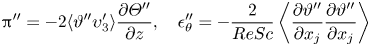 $$\begin{gather}{\rm \pi}'' ={-} 2 \langle \vartheta'' \upsilon_3' \rangle \frac{\partial \varTheta''}{\partial z}, \quad \epsilon_\theta'' ={-} \frac{2}{Re Sc} \left\langle \frac{\partial \vartheta''}{\partial x_j} \frac{\partial \vartheta''}{\partial x_j} \right\rangle \end{gather}$$
and the turbulent and diffusive fluxes
 $$\begin{gather} \varphi_u = \langle \vartheta \vartheta\, \upsilon_3 \rangle, \quad \varphi_\alpha ={-} \frac{1}{Re Sc} \frac{\partial \langle \vartheta \vartheta \rangle}{\partial z}, \end{gather}$$
 $$\begin{gather}\tilde{\varphi}_u = \langle \tilde{\vartheta} \tilde{\vartheta}\, \bar{\upsilon}_3 \rangle, \quad \tilde{\varphi}_\alpha ={-} \frac{1}{Re Sc} \frac{\partial \langle \tilde{\vartheta} \tilde{\vartheta} \rangle}{\partial z}, \end{gather}$$
 $$\begin{gather}\varphi_u'' = \langle \vartheta'' \vartheta''\, \upsilon_3' \rangle, \quad \varphi_\alpha'' ={-} \frac{1}{Re Sc} \frac{\partial \langle \vartheta'' \vartheta'' \rangle}{\partial z} . \end{gather}$$
As shown in figure 7(a), the turbulence production of scalar fluctuations is largely reduced for the scalar field  $\vartheta ''$ driven by the small-scale velocity field. This behaviour can be easily explained by considering that turbulence production is a large-scale anisotropic phenomenon and, hence, is largely inhibited when coupling a scalar field with an almost isotropic small-scale velocity field. Accordingly, the scalar field $\tilde {\vartheta }$ being driven by a very anisotropic large-scale velocity field exhibits a turbulence production that is almost unaltered with respect to that of $\vartheta$. The behaviour of turbulence dissipation is shown in the inset of figure 7(a). At the initial stages of the decay, the dissipations of both $\tilde {\vartheta }$ and $\vartheta ''$ show a reduction with respect to that of the scalar field $\vartheta$. On the other hand, for $t \ge 70$ only the dissipation of the scalar field $\vartheta ''$ shows a reduction while the dissipation of $\tilde {\vartheta }$ is found to almost recover the dissipation values of $\vartheta$.
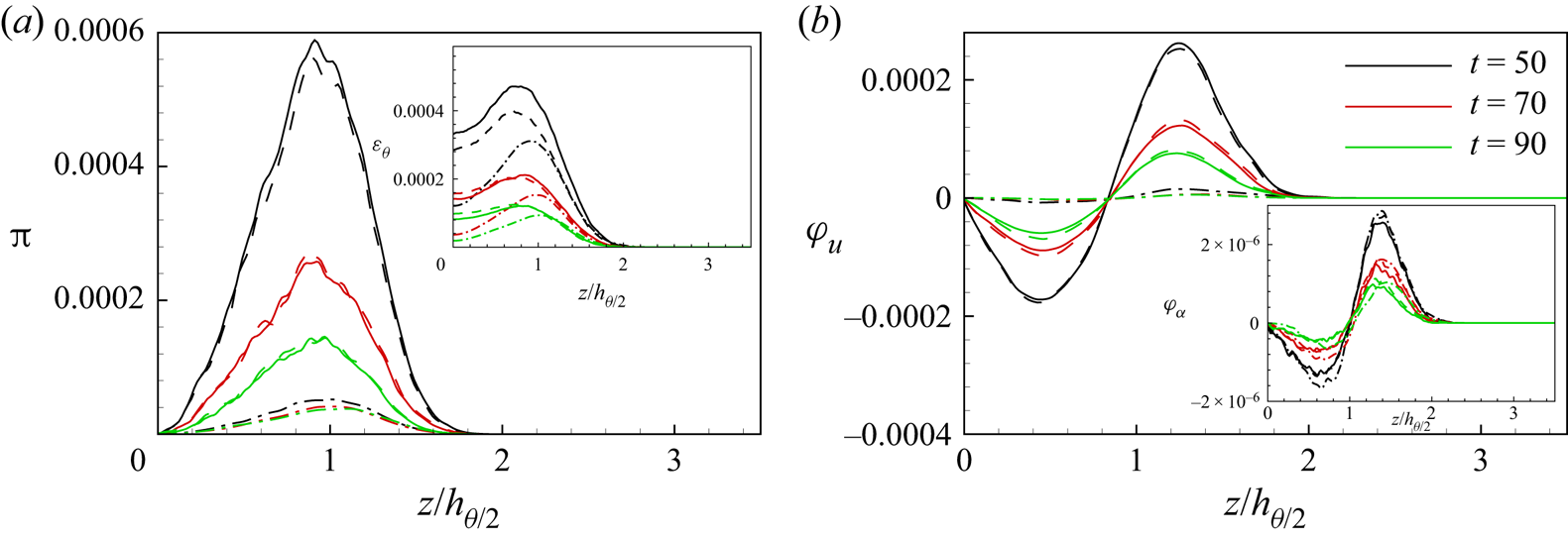
Figure 7. Scalar variance budget at  $t=50$, $70$ and $90$ for the scalar fields $\theta$ (solid line), $\tilde {\theta }$ (dashed line) and $\theta ''$ (dashed-dotted line). (a) Turbulence production and dissipation (inset). (b) Turbulent flux and diffusive flux (inset). The jet centreline distance $z$ is normalized with $h_{\theta /2}$ defined as the jet centreline distance where the mean scalar concentration reduces to half its centreline value.
These behaviours of turbulence production and dissipation can be used to explain the previously observed decays of the mean and variance of the scalar concentration (see again figure 6). By noting that the turbulence production of scalar fluctuations is a phenomenon that subtracts intensity from the mean field and releases it to the fluctuations, it is immediately clear that for the scalar field  $\theta ''$, the large reduction in the production of scalar fluctuations leads to a significantly slower decay of the mean scalar concentration $\varTheta ''(t)$. This reduction in the production of scalar fluctuations is not balanced by an equivalently large decrease of dissipation thus leading to a reduction of the net source of scalar fluctuations, i.e. ${\rm \pi} '' - \epsilon _\theta '' < {\rm \pi}- \epsilon _\theta$. As a consequence, a more rapid decay of the intensity of the scalar fluctuations $\langle \vartheta '' \vartheta '' \rangle (t)$ is observed. The opposite scenario occurs for the scalar $\tilde {\theta }$ driven by the anisotropic large-scale velocity field. In this case the production of scalar fluctuations is only marginally reduced, thus justifying the slightly slower decay of the mean scalar concentration $\tilde {\varTheta }(t)$. This slight reduction of production is combined with a larger reduction of dissipation especially at the first stages of the evolution, thus leading to an increase of the net source of scalar fluctuations, i.e. $\tilde {{\rm \pi} } - \tilde {\epsilon }_\theta > {\rm \pi}- \epsilon _\theta$. This behaviour justifies the observed slower decay of the intensity of the scalar fluctuations $\langle \tilde {\vartheta } \tilde {\vartheta }\rangle (t)$.
The formalism of the scalar variance budget allows us also to address the inertial and diffusive phenomena of spatial spreading of the scalar fluctuations from the production to the dissipative regions of the flow, i.e. the turbulent and diffusive fluxes  $\varphi _u$ and $\varphi _\alpha$. As shown in figure 7(b), the scalar fluctuations are transported from the production region towards the inner and outer regions of the jet, $z/h_{\theta /2} < 1$ and $z/h_{\theta /2} > 1$, respectively. This transport is essentially performed by inertial mechanisms for both $\vartheta$ and $\tilde {\vartheta }$, i.e. the scalar fluctuations driven by the unfiltered field and by the large-scale velocity field, respectively. Indeed, the turbulent flux is always far greater than the diffusive one: $\varphi _u \gg \varphi _\alpha$ and $\tilde {\varphi }_u \gg \tilde {\varphi }_\alpha$. The scenario is, however, different for the scalar fluctuations $\vartheta ''$ driven by the small-scale velocity field. Also in this case the fluctuations are mainly transported by inertial mechanisms, $\varphi _u'' > \varphi _\alpha ''$, but their intensity is markedly reduced: $\varphi _u'' \ll \varphi _u$. On the contrary, the diffusion mechanisms are found to surprisingly remain almost unaltered, i.e. $\varphi _\alpha '' \approx \varphi _\alpha$. Accordingly, we argue that the reduction of the inertial transport mechanisms is not induced by a decrease of the scalar fluctuation intensity given by the contraction of the turbulence production but simply by a less efficient coupling of the small-scale velocity field with the scalar fluctuations, i.e. $|\langle \vartheta '' \vartheta '' \upsilon _3' \rangle | \ll |\langle \vartheta \vartheta \, \upsilon _3 \rangle |$. As a result, the percentage contribution of diffusion with respect to advection in the spatial spreading of the scalar fluctuations $\vartheta ''$ is largely increased.
As expected, the described different evolution of the mean and fluctuating scalar field for the three numerical experiments also has an impact on the global mixing and entrainment properties of the scalar jet. In figure 8(a), the entrained volume  $\mathcal {V}$, defined as the volume of fluid where the scalar concentration is $\theta > \theta _{th}$ with $\theta _{th} = 0.02 \varTheta _{cl}$, is shown as a function of time for the three numerical experiments. During the flow decay, the entrained volume is significantly reduced for the scalar driven by the small-scale velocity field, $\mathcal {V}'' < \mathcal {V}$. On the other hand, a smaller reduction of the entrained volume is observed for the scalar driven by the large-scale velocity field, $\tilde {\mathcal {V}} < \mathcal {V}$. This difference between the two scalar fields $\tilde {\theta }$ and $\theta ''$ is enhanced when considering the spreading of the scalar jet. As shown in the inset of 8(a), the position of the scalar interface is only slightly reduced for the scalar driven by the large-scale velocity field, $\tilde {h}_\theta \approx h_\theta$, in contrast to the scalar driven by the small-scale velocity field where the position of the scalar interface advances very slowly, $h_\theta '' \ll h_\theta$.
Figure 8. (a) Temporal evolution of the entrained volume  $\mathcal {V}$ and of the position of the interface $h_\theta$ (inset) for the scalar field driven by the unfiltered velocity field $\mathcal {V}$ and $h_\theta$ (solid line), by the large-scale velocity field $\tilde {\mathcal {V}}$ and $\tilde {h}_\theta$ (dashed line) and by the small-scale velocity field $\mathcal {V}''$ and $h_\theta ''$ (dashed-dotted line). (b) Probability density function of the scalar fields $\theta$, $\tilde {\theta }$ and $\theta ''$ evaluated for $t=120$ at the mean scalar interface position $z=h_\theta$, $z=\tilde {h}_\theta$ and $z=h_\theta ''$ and at the jet centreline $z=0$ (inset).
The different entrainment and propagation of the scalars  $\tilde {\theta }$ and $\theta ''$ can be explained by recalling the behaviours of the turbulent and diffusive fluxes. Contrary to the scalar $\tilde {\theta }$, the scalar driven by the small-scale velocity field $\theta ''$ is characterized by a significantly reduced inertial flux, $|\varphi _u''| \ll |\varphi _u|$, thus explaining the very slow spreading of the jet, $h_\theta '' \ll h_\theta$. We argue that, associated with this reduction of inertial fluxes, a reduced amount/intensity of entrapment events is experienced by the scalar $\theta ''$. As a result, the presence and the size of null-concentration blobs entrapped within the scalar jet $z < h_\theta ''$ are markedly reduced. At the same time the diffusion processes for the scalar $\theta ''$ remain almost unaltered, $\varphi _\alpha '' \approx \varphi _\alpha$. Hence, we argue that the time scale of the diffusion processes is small enough to effectively complete the entrainment of the reduced amount of entrapped null-concentration blobs. This picture is confirmed by figure 5, where the instantaneous flow patterns of the scalar field $\theta ''$ show a significantly more mixed flow region within the scalar jet $z < h_\theta ''$. These behaviours are not observed for the scalar driven by the large-scale velocity field $\tilde {\theta }$ since in this case engulfment events are largely reproduced $\tilde {\varphi }_u \gg \varphi _u''$ while retaining the same intensity of the diffusion processes $\tilde {\varphi }_\alpha \approx \varphi _\alpha ''$. Indeed, the pattern of the scalar $\tilde {\theta }$ shown in figure 5 exhibits a number of unmixed flow regions within the scalar jet $z < \tilde {h}_\theta$. This different behaviour of entrainment for the two scalars explains why the reduction of the entrained volume for the scalar $\theta ''$, $\mathcal {V}'' < \mathcal {V}$, is not as large as the reduction of the spreading of the jet, $h_\theta '' \ll h_\theta$.
The probability density function of the three scalars  $\vartheta$, $\tilde {\vartheta }$ and $\vartheta ''$ actually confirms the above mentioned entrainment and mixing properties. As shown in the inset of figure 8(b), the probability density function at the jet centreline highlights a symmetric distribution of the scalar fluctuations for $\vartheta ''$ and a very wide and asymmetric distribution for $\vartheta$ and $\tilde {\vartheta }$. In particular, this asymmetry is essentially given by an increased probability of large negative scalar fluctuations that can be clearly associated with the presence of unmixed flow regions of low scalar concentration even at the jet centreline due to very-large-scale engulfment events. In this respect, it can be noticed that the probability density functions of $\vartheta$ and $\tilde {\vartheta }$ have a negative tail that extends up to $\vartheta /\varTheta = -1$ corresponding to $\theta = 0$ and, hence, to completely unmixed flow regions. This behaviour is not observed for $\vartheta ''$, thus confirming that this field lacks engulfment events and, at the same time, exhibits a mixed flow in the scalar jet core.
As shown in figure 8(b), the scenario is completely different at the scalar interface,  $z=h_\theta$, $z=\tilde {h}_\theta$ and $z=h_\theta ''$. In this case, all three scalar fields $\vartheta$, $\tilde {\vartheta }$ and $\vartheta ''$ show a peak of probability for $\vartheta /\varTheta = -1$ corresponding again to $\theta = 0$. Indeed, the presence of entrainment at the scalar interface is revealed by a wide positive tail of the probability distribution. Interestingly, for the scalars $\vartheta$ and $\tilde {\vartheta }$ this positive tail is very wide and flat, thus revealing that at the scalar interface a wide range of scalar fluctuation intensities is almost equally probable. We argue that this plateau is again due to large-scale engulfment mechanisms that intersect the mean scalar interface and contain a wide range of scalar values. On the contrary, the scalar $\vartheta ''$ driven by the small-scale velocity field exhibits a positive tail characterized by a decrease of the probability with the intensity of the scalar fluctuations. Indeed, in this case engulfment is absent and the small scales of nibbling can contain only a fraction of the entire range of scalar values.
6. Turbulent entrainment and mixing
6.1. Theoretical framework
The different mixing and entrainment properties of the three numerical experiments highlighted in the previous section can now be analysed in terms of heuristic arguments in order to reveal the essential features of the process. In § 3, we have shown how the complex dynamics of turbulent fluctuations has an impact on the entrainment and mixing rates of a scalar field by establishing the geometrical and fluctuating properties of the scalar surface through which a scalar concentration flux occurs following the well-established Fick's law of diffusion. We apply now these arguments to the three scalar concentration experiments here developed.
In the case of a temporal planar jet and considering the scalar iso-concentration surface  $\theta = 0.02 \varTheta _{cl}$, a proper choice of the characteristic scales for the diffusive and inertial scalar fluxes (3.4) and (3.5) is
 \begin{equation} L = h_\theta, \quad \ell = \eta_{int}^\theta, \quad u_\ell = u_{\eta_{int}}, \quad \mathcal{C} = \varTheta_{cl}, \end{equation}
where  $h_\theta$ is the jet half-width defined by the mean scalar interface itself, while $\eta _{int}^\theta$ and $u_{\eta _{int}}$ are the Batchelor scale and the Kolmogorov velocity evaluated at the scalar interface $z = h_\theta$. Without loss of generality we have chosen the scalar iso-concentration surface $\theta = 0.02 \varTheta _{cl}$, but let us highlight that the same theoretical framework applies for all scalar surfaces. With these characteristic scales, the diffusive and inertial fluxes become
 \begin{equation} \phi_\alpha = \alpha \frac{\varTheta_{cl}}{\eta_{int}^\theta} S_0 \left ( \frac{\eta_{int}^\theta}{h_\theta} \right )^{2-D}, \quad \phi_{u} = \varTheta_{cl} u_{\eta_{int}} S_0 \left ( \frac{\eta_{int}^\theta}{h_\theta} \right )^{2-D} \end{equation}
and it is easy to show that the two fluxes equal each other:
 \begin{equation} \phi_\alpha = \phi_{u} . \end{equation}
An alternative scaling is given by considering an outer velocity scale in the assumptions (6.1a–d), i.e.
 \begin{equation} u_\ell = \upsilon_{int}, \end{equation}
where  $\upsilon _{int}$ is the standard deviation of the velocity fluctuations at $z = h_\theta$. In this case, the inertial flux differs from the diffusive one and can be written as
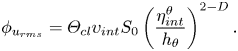 \begin{equation} \phi_{u_{rms}} = \varTheta_{cl} \upsilon_{int} S_0 \left ( \frac{\eta_{int}^\theta}{h_\theta} \right )^{2-D} . \end{equation}
In the temporal jet, the entrainment hypothesis (3.7) can be written as
 \begin{equation} \phi = S_0 V_\theta \varTheta_{cl}, \end{equation}
where  $S_0$ is the ( $x$–
$x$– $y$)-plane surface of the jet. Hence, the different estimates of the scalar surface velocity become
 \begin{equation} \left.\begin{gathered}
V_\theta^\alpha =
V_\theta^{u} = \frac{\alpha}{\eta_{int}^\theta} \left (
\frac{\eta_{int}^\theta}{h_\theta} \right )^{2-D} =
u_{\eta_{int}} \left ( \frac{\eta_{int}^\theta}{h_\theta}
\right )^{2-D},\\
V_\theta^{u_{rms}} = \upsilon_{int}
\left ( \frac{\eta_{int}^\theta}{h_\theta} \right )^{2-D}.\end{gathered}\right\}
\end{equation}
\begin{equation} \left.\begin{gathered}
V_\theta^\alpha =
V_\theta^{u} = \frac{\alpha}{\eta_{int}^\theta} \left (
\frac{\eta_{int}^\theta}{h_\theta} \right )^{2-D} =
u_{\eta_{int}} \left ( \frac{\eta_{int}^\theta}{h_\theta}
\right )^{2-D},\\
V_\theta^{u_{rms}} = \upsilon_{int}
\left ( \frac{\eta_{int}^\theta}{h_\theta} \right )^{2-D}.\end{gathered}\right\}
\end{equation}
In the self-similar regime,  $h_\theta \propto \sqrt {t}$, $\eta _{int}^\theta \propto \sqrt {t}$, $u_{\eta _{int}} \propto 1/\sqrt {t}$ and $\upsilon _{int} \propto 1/\sqrt {t}$, thus leading to the following scaling:
 \begin{equation} V_\theta= V_\theta^\alpha = V_\theta^{u} \propto \frac{1}{\sqrt{t}}, \quad V_\theta^{u_{rms}} \propto \frac{1}{\sqrt{t}} . \end{equation}
 For the scalar  $\tilde {\theta }$ driven by the large-scale velocity field, the above assumptions apply by simply replacing the characteristic scales, i.e.
 \begin{equation} L = \tilde{h}_\theta,\quad \ell = \tilde{\eta}_{int}^\theta, \quad \mathcal{C} = \tilde{\varTheta}_{cl}, \quad u_\ell = \tilde{u}_{\eta_{int}} \quad \text{or} \quad u_\ell = \tilde{\upsilon}_{int}, \end{equation}
thus leading to the following velocity scales:
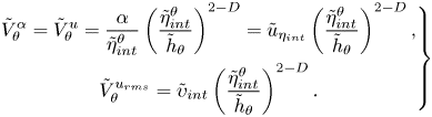 \begin{equation} \left.\begin{gathered} \tilde{V}_\theta^\alpha = \tilde{V}_\theta^{u} = \frac{\alpha}{\tilde{\eta}_{int}^\theta} \left ( \frac{\tilde{\eta}_{int}^\theta}{\tilde{h}_\theta} \right )^{2-D} = \tilde{u}_{\eta_{int}} \left ( \frac{\tilde{\eta}_{int}^\theta}{\tilde{h}_\theta} \right )^{2-D},\\ \tilde{V}_\theta^{u_{rms}} = \tilde{\upsilon}_{int} \left ( \frac{\tilde{\eta}_{int}^\theta}{\tilde{h}_\theta} \right)^{2-D}.\end{gathered}\right\} \end{equation}
On the contrary, for the scalar  $\theta ''$ driven by the small-scale velocity field, the choice of the characteristic scales needs more attention. Indeed, due to the absence of large-scale engulfment events, the largest characteristic length for the scalar surface is given by the filter length $\varDelta$ (see the instantaneous scalar topology shown in figure 5). Accordingly, the characteristic scales are
 \begin{equation} L = \varDelta, \quad \ell = \eta_{int}^{\theta \,\prime\prime}, \quad \mathcal{C} = \varTheta_{cl}'', \quad u_\ell = u_{\eta_{int}}'' \quad \text{or} \quad u_\ell = \upsilon_{int}'' \end{equation}
and the estimates of the scalar surface velocity become
 \begin{equation} \left.\begin{gathered}
{V_\theta^\alpha}^{\prime\prime} = {V_\theta^{u}}^{\prime
\prime} = \frac{\alpha}{\eta_{int}^{\theta \,
\prime\prime}} \left ( \frac{\eta_{int}^{\theta \,
\prime\prime}}{\varDelta} \right )^{2-D} = u_{\eta_{int}}
'' \left ( \frac{\eta_{int}^{\theta \,
\prime\prime}}{\varDelta} \right )^{2-D},\\
{V_\theta^{u_{rms}}}^{\prime \prime} = \upsilon_{int}''
\left ( \frac{\eta_{int}^{\theta \,
\prime\prime}}{\varDelta} \right )^{2-D} .
\end{gathered}\right\}
\end{equation}
\begin{equation} \left.\begin{gathered}
{V_\theta^\alpha}^{\prime\prime} = {V_\theta^{u}}^{\prime
\prime} = \frac{\alpha}{\eta_{int}^{\theta \,
\prime\prime}} \left ( \frac{\eta_{int}^{\theta \,
\prime\prime}}{\varDelta} \right )^{2-D} = u_{\eta_{int}}
'' \left ( \frac{\eta_{int}^{\theta \,
\prime\prime}}{\varDelta} \right )^{2-D},\\
{V_\theta^{u_{rms}}}^{\prime \prime} = \upsilon_{int}''
\left ( \frac{\eta_{int}^{\theta \,
\prime\prime}}{\varDelta} \right )^{2-D} .
\end{gathered}\right\}
\end{equation}
6.2. Comparison with the numerical experiments
To verify these scalings, it is important to note that the entrainment velocity  $V_e$ is null in the temporal jet, since
 \begin{equation} \frac{\textrm{d}}{\textrm{d}t} \int U \,\textrm{d}z = 0, \end{equation}
and, hence, the relative speed of scalar interface defined in (3.6) is entirely determined by the boundary entrainment rate  $V_\theta = V_b$. The boundary entrainment velocity can be computed as the rate of variation of the volume of fluid entrained $\mathcal {V}$:
 \begin{equation} V_b = \frac{1}{2 S_0} \frac{\textrm{d}\mathcal{V}}{\textrm{d}t}. \end{equation}
In figure 9(a), the behaviour of the boundary entrainment velocity for the three numerical experiments is shown. In accordance with the flow analysis reported in § 5, the scalar field  $\tilde {\theta }$ exhibits only a slight reduction of the entrainment rate, while, for the scalar field $\theta ''$, this reduction is larger. As shown in the inset of figure 9(a), after an initial transient that is more marked for the scalar field $\theta ''$, a self-similar scaling $V_b \propto t^{-1/2}$ applies for $t > 80$.

Figure 9. (a) Boundary entrainment rate as a function of time for the three scalar fields  $\theta$, $\tilde {\theta }$ and $\theta ''$. The inset shows the entrainment rate scaled in self-similar variables. (b) Time evolution of the scalar surface area computed using the fractal estimate (6.15a–c) for the three scalar fields $\theta$, $\tilde {\theta }$ and $\theta ''$.
The heuristic approach defined in the previous section is based on the idea that iso-surfaces are determined by the structure of turbulence and are fractal-like (Sreenivasan et al. Reference Sreenivasan, Ramshankar and Meneveau1989). The estimate of the corresponding iso-surface area for the three numerical experiments is reported in figure 9(b). Let us recall that for the assumptions made in the previous section, the fractal-like surfaces read
 \begin{equation} S_\ell = S_0 \left ( \frac{\eta_{int}^\theta}{h_\theta} \right )^{2-D}, \quad \tilde{S}_\ell = S_0 \left ( \frac{\tilde{\eta}_{int}^\theta}{\tilde{h}_\theta} \right )^{2-D}, \quad S_\ell'' = S_0 \left ( \frac{\eta_{int}^{\theta \, \prime\prime}}{\varDelta} \right )^{2-D}, \end{equation}
respectively, for the scalar fields  $\theta$, $\tilde {\theta }$ and $\theta ''$. As shown in figure 9(b), both the scalar fields $\tilde {\theta }$ and $\theta ''$ experience a reduction of the scalar interface area. In the $\tilde {\theta }$ scalar field, this reduction is given by the lack of small-scale wrinkles at the scalar interface due to the absence of small-scale nibbling. Conversely, in the $\theta ''$ scalar field, this reduction is caused by the lack of large-scale convolutions of the scalar interface due to the absence of large-scale engulfment. Since this reduction is larger for the scalar field $\theta ''$, $S_\ell '' < \tilde {S}_\ell < S_\ell$, we argue that large-scale engulfment more efficiently increases the interface area than small-scale nibbling. Let us notice that we have verified these scalings by measuring the actual iso-surface area of $\theta = \theta _{th}$ and a good agreement has been found. The behaviour of the scalar interface areas supports the observed reduction of entrainment rate for the scalar fields $\tilde {\theta }$ and $\theta ''$ (see again figure 9a). But, actually, the physics at the basis of the rate of entrainment is more complex and eludes the simple indication given by the interface area. Indeed, the heuristic models for the entrainment rate (6.7a,b), (6.10a,b) and (6.12), despite being based on the fractal surface area, actually show a completely different behaviour. Let us try to grasp the essential reasons.
In figure 10(a,b), the predictions of the entrainment velocity given by (6.7a,b), (6.10a,b) and (6.12) are shown. For the scalars  $\theta$ and $\tilde {\theta }$, respectively driven by the unfiltered and large-scale velocity fields, the predictions are reasonable in terms of both behaviour and reduction of the entrainment rate for the scalar $\tilde {\theta }$. Compare these behaviours with the measurements reported in figure 9(a). On the other hand, the prediction for the scalar $\theta ''$ lacks in capturing the reduction of the entrainment rate that, on the contrary, is estimated to be the largest one. Despite being characterized by the largest predicted reduction of the scalar iso-surface area, see figure 9(b), equations (6.12) predict a large entrainment rate because of a smaller value of the Batchelor scale and of a larger value of the velocity fluctuation intensity, i.e.
 \begin{equation} \eta_{int}^{\theta \, \prime\prime} \ll \eta_{int}^\theta \quad \text{and} \quad \upsilon_{int}'' \gg \upsilon_{int} . \end{equation}
These inequalities are simply due to the lower propagation rate of the scalar field  $\theta ''$ with respect to $\theta$ and $\tilde {\theta }$. As a result, the interface of the scalar field $\theta ''$ experiences a velocity field associated with a much more inner location with respect to that experienced by the other two scalar interfaces since $h_\theta '' \ll \tilde {h}_\theta \approx h_\theta$. At inner positions, the variance and dissipation of velocity fluctuations are larger than those at the outer regions of the jet (see (Cimarelli et al. Reference Cimarelli, Mollicone, van Reeuwijk and De Angelis2021)) and the operation of filtering out the large-scale fluctuations is not able to balance this flow inhomogeneity thus justifying inequalities (6.16a,b). Overall, we have that the scalar $\theta ''$ driven by the small-scale velocity field experiences a reduction of the scalar interface area $S_\ell '' < \tilde {S}_\ell < S_\ell$ that is overcome by a larger increase of the diffusion velocity $\alpha / \eta _{int}^{\theta \, \prime \prime } \gg \alpha / \tilde {\eta }_{int}^\theta \approx \alpha / \eta _{int}^\theta$ and of the velocity fluctuations $\upsilon _{int}'' \gg \tilde {\upsilon }_{int} \approx \upsilon _{int}$. For this reason, (6.7a,b), (6.10a,b) and (6.12) actually predict a larger entrainment rate for the scalar $\theta ''$.
6.3. Heuristic refinement of the entrainment and mixing assumptions
Evidently, the heuristic assumptions at the basis of (6.7a,b), (6.10a,b) and (6.12) miss some relevant physical processes. We try here to grasp the essential aspects.
Let us start with the scalar diffusion. The hypothesis (6.2a,b),
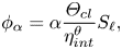 \begin{equation} \phi_\alpha = \alpha \frac{\varTheta_{cl}}{\eta_{int}^\theta} S_\ell, \end{equation}
certainly works for the scalar fields  $\theta$ and $\tilde {\theta }$ but not for $\theta ''$. Indeed, for the latter, the decrease in the scalar surface area, $S_\ell '' < \tilde {S}_\ell < S_\ell$, is overcome by a larger increase of the characteristic scalar gradient,
 \begin{equation} \frac{\varTheta_{cl}''}{\eta_{int}^{\theta \, \prime\prime}} \gg \frac{\tilde{\varTheta}_{cl}}{\tilde{\eta}_{int}^\theta} \approx \frac{\varTheta_{cl}}{\eta_{int}^\theta}, \end{equation}
due both to a slower decay of the mean scalar concentration  $\varTheta _{cl}'' \gg \tilde {\varTheta }_{cl} \approx \varTheta _{cl}$ (see figure 6a) and to an inner location of the scalar interface that in turn leads to $\eta _{int}^{\theta \, \prime \prime } \ll \tilde {\eta }_{int}^\theta \approx \eta _{int}^\theta$. It appears that the mean scalar concentration is a valid indicator of the scalar fluctuation intensity for the fields $\theta$ and $\tilde {\theta }$ but not for $\theta ''$. Indeed, the increase of mean scalar concentration $\tilde {\varTheta }_{cl}$ is associated with an increase also of the scalar fluctuation intensity $\langle \tilde {\vartheta }\tilde {\vartheta } \rangle _{cl}$ (see figure 6(a,b). On the contrary, the increase of mean scalar concentration $\varTheta _{cl}''$ is associated with a decrease of the scalar fluctuation intensity $\langle \vartheta '' \vartheta '' \rangle _{cl}$ (see again figure 6a,b). In practical applications, this different behaviour could be ascribed for example to the presence of external agents or chemical reactions. Accordingly, since the scalar fluctuation intensity could not be directly related to the behaviour of the mean scalar concentration, it is important to directly take it into account in the scalar diffusion expression:
 \begin{equation} \phi_\alpha = \alpha \frac{\sqrt{\langle \vartheta \vartheta \rangle_{cl}}}{\eta_{int}^\theta} S_\ell . \end{equation}
This expression leads to the following velocities:
 \begin{equation} \left.\begin{gathered}
V_\theta^\alpha = \alpha \frac{\sqrt{\langle \vartheta
\vartheta \rangle_{cl}} /
\varTheta_{cl}}{\eta_{int}^\theta} \frac{S_\ell}{S_0},\\
\tilde{V}_\theta^\alpha = \alpha \frac{\sqrt{\langle
\tilde{\vartheta} \tilde{\vartheta} \rangle_{cl}} /
\tilde{\varTheta}_{cl}}{\tilde{\eta}_{int}^\theta}
\frac{\tilde{S}_\ell}{S_0}, \\
{V_\theta^\alpha}^{\prime\prime} = \alpha
\frac{\sqrt{\langle \vartheta'' \vartheta'' \rangle_{cl}} /
\varTheta_{cl}''}{\eta_{int}^{\theta \, \prime\prime}}
\frac{S_\ell''}{S_0}, \end{gathered}\right\}
\end{equation}
\begin{equation} \left.\begin{gathered}
V_\theta^\alpha = \alpha \frac{\sqrt{\langle \vartheta
\vartheta \rangle_{cl}} /
\varTheta_{cl}}{\eta_{int}^\theta} \frac{S_\ell}{S_0},\\
\tilde{V}_\theta^\alpha = \alpha \frac{\sqrt{\langle
\tilde{\vartheta} \tilde{\vartheta} \rangle_{cl}} /
\tilde{\varTheta}_{cl}}{\tilde{\eta}_{int}^\theta}
\frac{\tilde{S}_\ell}{S_0}, \\
{V_\theta^\alpha}^{\prime\prime} = \alpha
\frac{\sqrt{\langle \vartheta'' \vartheta'' \rangle_{cl}} /
\varTheta_{cl}''}{\eta_{int}^{\theta \, \prime\prime}}
\frac{S_\ell''}{S_0}, \end{gathered}\right\}
\end{equation}
respectively, for the scalar fields  $\theta$, $\tilde {\theta }$ and $\theta ''$. As shown in figure 10(c), these are actually able to predict the reduction of entrainment for both the scalar fields $\tilde {\theta }$ and $\theta ''$.


We consider now the inertial scalar flux. The hypothesis (6.5),
 \begin{equation} \phi_{u_{rms}} = \varTheta_{cl} \upsilon_{int} S_\ell, \end{equation}
certainly works for the scalar fields  $\theta$ and $\tilde {\theta }$ but not for $\theta ''$. Indeed, for the latter, the decrease in the scalar surface area, $S_\ell '' < \tilde {S}_\ell < S_\ell$, is overcome by a larger increase of the velocity fluctuations,
 \begin{equation} \upsilon_{int}'' \gg \tilde{\upsilon}_{int} \approx \upsilon_{int}, \end{equation}
due to the inner location of the scalar interface for  $\theta ''$. Hence, contrary to measurements, a larger velocity of propagation of the scalar $\theta ''$ is predicted. This behaviour actually suggests that the global intensity of the velocity fluctuations is not a complete indicator for the transport of scalar fluctuations. Evidently, the scalar transport is not accomplished efficiently by all the scales of the turbulent spectrum. The main difference between the intensity of the velocity fluctuations $\tilde {\upsilon }_{int}$ and $\upsilon _{int}''$ is given by the velocity scales involved. The intensity $\tilde {\upsilon }_{int}$ is produced by an anisotropic field of motion characterized by large-scale engulfment events while the intensity $\upsilon _{int}''$ is produced by essentially isotropic small-scale fluctuations. It is then possible to argue that only the anisotropic part of the velocity field significantly contributes to the net propagation of scalars in agreement with a number of recent works (Cimarelli et al. Reference Cimarelli, Cocconi, Frohnapfel and De Angelis2015, Reference Cimarelli, Mollicone, van Reeuwijk and De Angelis2021; Buxton, Breda & Dhall Reference Buxton, Breda and Dhall2019). Accordingly, we introduce the isotropy indicator
 \begin{equation} \gamma = \frac{\sqrt{\langle \upsilon_3 \upsilon_3 \rangle}}{\sqrt{\langle \upsilon_1 \upsilon_1 \rangle} + \sqrt{\langle \upsilon_2 \upsilon_2 \rangle} + \sqrt{\langle \upsilon_3 \upsilon_3 \rangle}} . \end{equation}
This parameter tends to 1 when the intensity of the fluctuations is increasingly contained in the cross-flow component and diminishes when the anisotropic state departs from the one-component condition by reaching 1/3 corresponding to isotropic conditions. In velocity fields characterized by large-scale engulfment events,  $\gamma > 1/3$, and, hence, it can be used to identify the portion of the intensity of the velocity fluctuations that is active in the scalar propagation. Accordingly, the inertial scalar flux can be rewritten as
 \begin{equation} \phi_{u_{rms}} = \varTheta_{cl} (\gamma - \tfrac{1}{3} ) \upsilon_{int} S_\ell \end{equation}
and the entrainment velocities read
 \begin{equation} \left.\begin{gathered}
V_\theta^{u_{rms}} = \left(\gamma - \frac{1}{3} \right)
\upsilon_{int} \frac{S_\ell}{S_0},\\
\tilde{V}_\theta^{u_{rms}} = \left(\tilde{\gamma} -
\frac{1}{3} \right) \tilde{\upsilon}_{int}
\frac{\tilde{S}_\ell}{S_0},\\ {V_\theta^{u_{rms}}}^{\prime
\prime} = \left(\gamma'' - \frac{1}{3} \right)
\upsilon_{int}'' \frac{S_\ell''}{S_0},
\end{gathered}\right\}
\end{equation}
\begin{equation} \left.\begin{gathered}
V_\theta^{u_{rms}} = \left(\gamma - \frac{1}{3} \right)
\upsilon_{int} \frac{S_\ell}{S_0},\\
\tilde{V}_\theta^{u_{rms}} = \left(\tilde{\gamma} -
\frac{1}{3} \right) \tilde{\upsilon}_{int}
\frac{\tilde{S}_\ell}{S_0},\\ {V_\theta^{u_{rms}}}^{\prime
\prime} = \left(\gamma'' - \frac{1}{3} \right)
\upsilon_{int}'' \frac{S_\ell''}{S_0},
\end{gathered}\right\}
\end{equation}
respectively, for the scalar fields  $\theta$, $\tilde {\theta }$ and $\theta ''$. As shown in figure 10(d), these predictions of the scalar entrainment velocity are actually able to predict the reduction of entrainment for both the scalar fields $\tilde {\theta }$ and $\theta ''$. Let us finally notice that these predictions are based on scaling arguments and, hence, are intended to give a good qualitative rather than a quantitative description of the boundary entrainment rate of figure 9(a).
7. Conclusions
The entrainment and mixing processes of scalar fields are investigated for the symmetries of an incompressible temporal planar jet. For Schmidt numbers close to unity, both mixing due to turbulence and scalar diffusion occur with similar time scales. In particular, scalar diffusion processes create a flux through scalar iso-concentration surfaces whose geometrical and fluctuating properties are prescribed by the complex dynamics of turbulence, thus forming coupled mechanisms of entrainment which elude a clear understanding. The definition of two scalar fields separately driven by large- and small-scale fluctuations is a sound starting point to address this issue. To this aim, numerical experiments have been conducted in order to establish from a dynamical point of view the scale dependency of turbulence mixing and entrainment of a passive scalar. Three independent scalar fields have been solved,  $\theta$, $\tilde {\theta }$ and $\theta ''$, respectively driven by the unfiltered motion and by the large- and small-scale velocity fields defined by the filter length $\varDelta = 2.2 \lambda _{cl}$. The large-scale field is found to capture the large-scale anisotropic engulfment events while the small-scale field retains only the small-scale motions commonly associated with nibbling.
We found that the evolution of the scalar field  $\tilde {\theta }$ is almost unaltered with respect to that of $\theta$. The propagation of the scalar field is only slightly reduced $\tilde {h}_\theta \approx h_\theta$ and the main difference is given by an increased number of unmixed flow regions within the jet core that leads to a reduced amount of entrained volume, $\tilde {\mathcal {V}} < \mathcal {V}$. Accordingly, it is found that both the inertial and diffusive scalar fluxes are almost unaltered, $\tilde {\varphi }_u \approx \varphi _u$ and $\tilde {\varphi }_\alpha \approx \varphi _\alpha$, thus showing that anisotropic large-scale fluctuations are responsible for almost the entire mechanism of scalar mixing. On the contrary, the small-scale velocity field driving the scalar $\theta ''$ does not capture engulfment events. In this case, the inertial fluxes are markedly reduced, $\varphi _u'' \ll \varphi _u$, thus showing that small-scale isotropic fluctuations do not contribute significantly to the process. As a result, the spreading of the jet is markedly reduced, $h_\theta '' \ll h_\theta$. On the other hand, the diffusive mechanisms are almost unaltered, $\varphi _\alpha '' \approx \varphi _\alpha$, and, together with the absence of large-scale engulfment, allows for a more complete mixing of the scalar jet core by diffusion thus leading to a reduction of the entrained volume $\mathcal {V}'' < \mathcal {V}$ that is less pronounced than the reduction of the spreading of the jet $h_\theta '' \ll h_\theta$.
Overall, we found that inertial fluxes guided by large-scale anisotropic phenomena of engulfment initiate the processes of scalar entrainment and mixing and essentially commit their strength to be further processed through a cascade process by nibbling mechanisms at small scales. Hence, this last stage does not prescribe the amount of entrainment and mixing, but essentially adapts itself to the conditions imposed by the large-scale features of the velocity field. This is also demonstrated by the fact that the evolution of the scalar fields  $\tilde {\theta }$ and $\theta ''$ diverges from the very beginning, $t=40$, where only the velocity field is significantly changed. We also argue that the velocity stirring of the scalar iso-concentration surfaces is more effectively accomplished by large-scale engulfment events than by small-scale nibbling. Indeed, we estimate that large-scale convolutions of the scalar iso-surface are responsible for a larger increase of the iso-surface area than small-scale wrinkles.
From a heuristic point of view, classical arguments lead to an entrainment velocity that is proportional to the intensity of the velocity fluctuations measured at the scalar surface times its area. These arguments actually fail in predicting the behaviour of the scalar field  $\theta ''$. Indeed, due to the lower rate of propagation, the scalar interface for $\theta ''$ experiences very large velocity fluctuations, $\upsilon _{int}'' \gg \tilde {\upsilon }_{int} \approx \upsilon _{int}$, but the velocity of entrainment is actually reduced. This phenomenon actually suggests that only the large-scale portion of the turbulent spectrum is actually active for scalar propagation. Accordingly, we found that the small-scale isotropic structure of the velocity field driving the scalar $\theta ''$ is essentially inactive for the scalar entrainment despite its intensity being large. On the contrary, the large-scale anisotropic motion driving the scalar $\tilde {\theta }$ is almost entirely active, thus leading to a larger velocity of propagation even if the intensity of its fluctuations is smaller. The adoption of a simple isotropy indicator to model the active fraction of the velocity fluctuations confirms this conjecture. The large-scale coherent structure of engulfment imposes the rate of entrainment more efficiently with respect to small-scale eddies by activating intense inertial fluxes and by setting the geometry and the area of the scalar surface.
It is worth noting that the present results are relevant also for reduced-order approaches to scalar mixing, in particular for large-eddy simulation where only the large scales of the velocity field are resolved. The present numerical experiments show that the scalar mixing processes are almost unaltered when driven solely by the large scales of the velocity field. Only a lack of scalar mixing in the jet core is observed that, however, can be recovered by simply adding a turbulent diffusivity to the scalar equation using classical gradient-diffusion hypothesis.
In closing this work, let us mention that the considered Reynolds number is rather low,  $Re_\lambda = 60$. By increasing the Reynolds number, the ratio between inviscid and viscous phenomena may change as long as a larger separation of scales is achieved. This aspect should be taken into account for future investigations.
Acknowledgements
We acknowledge the Italian supercomputing centre CINECA that, under the ISCRA C project NEXT (Numerical EXperiments on Turbulent entrainment), provided the high-performance computing resources for the present work. A.C. acknowledges G. Cocconi for his contribution to the preliminary study of this work. The authors would like to acknowledge also M. van Reeuwijk and E. De Angelis for useful discussions about the work.
Declaration of interests
The authors report no conflict of interest.
Appendix. Dataset validation
To validate the dataset used in the present work, a comparison with recent direct numerical simulation data of a turbulent temporal jet by Cimarelli et al. (Reference Cimarelli, Mollicone, van Reeuwijk and De Angelis2021) is here reported. The initial and boundary conditions are the same for both simulations with the exception of the Reynolds number:  $Re = 2000$ in Cimarelli et al. (Reference Cimarelli, Mollicone, van Reeuwijk and De Angelis2021) and $Re=3000$ in the present work. The two simulations differ in the numerical schemes, the domain extension and the spatial and temporal resolution adopted. The numerical code used in Cimarelli et al. (Reference Cimarelli, Mollicone, van Reeuwijk and De Angelis2021) is less accurate being based on a fourth-order-accurate spatial discretization and a third-order Adams–Bashforth scheme for time integration (see Craske & van Reeuwijk Reference Craske and van Reeuwijk2015; Verstappen & Veldman Reference Verstappen and Veldman2003). On the other hand, the domain lengths in the streamwise and spanwise directions and the spatial resolution are improved with respect to the present settings (see table 1). Despite these differences, the agreement between the two numerical datasets is very good. As shown in figure 11, the temporal behaviours of the mean centreline velocity $U_{cl}$ and of the mean centreline scalar concentration $\varTheta _{cl}$ predicted by the two simulations are essentially the same. A very good agreement is also observed in the cross-flow distribution of the numerical solutions as shown in figure 12 where the mean and variance profiles of velocity and scalar concentration are reported in self-similar variables, i.e. by re-scaling velocity with $U_{cl}$, scalar concentration with $\varTheta _{cl}$ and cross-flow position with the jet half-width $z_{1/2}$ defined as the centreline distance at which the mean velocity profile reduces to half its centreline value.

Figure 11. Temporal evolution of the mean centreline velocity  $U_{cl}$ and of the mean scalar concentration $\varTheta _{cl}$ for the present dataset (black lines) and for the reference dataset from Cimarelli et al. (Reference Cimarelli, Mollicone, van Reeuwijk and De Angelis2021) (red lines).

Figure 12. Velocity and scalar self-similar scalings for the present dataset (black lines) and for the reference dataset from Cimarelli et al. (Reference Cimarelli, Mollicone, van Reeuwijk and De Angelis2021) (red lines). (a) Mean velocity and turbulent kinetic energy profiles. (b) Scalar mean and variance profiles.
Table 1. Numerical settings of the present simulation compared to those of the reference simulation by Cimarelli et al. (Reference Cimarelli, Mollicone, van Reeuwijk and De Angelis2021). For the simulation by Cimarelli et al. (Reference Cimarelli, Mollicone, van Reeuwijk and De Angelis2021), the time step is variable and prescribed by the condition  $\textrm {CFL} < 0.3$; hence, the value reported is the average time step used. It is important to note that the values of the Reynolds number and of the domain extension here reported for the simulation of Cimarelli et al. (Reference Cimarelli, Mollicone, van Reeuwijk and De Angelis2021) differ from those reported in their work because the reference length $H$ used for non-dimensionalization was defined as half the initial jet width contrary to the entire initial width considered here (see § 2.1).
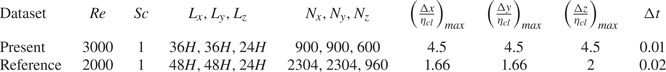


 Open access