


1. Introduction
The periodic formation, growth, detachment and advection of partial cavities is termed cloud cavitation. This phenomenon is associated with performance degradation, erosion and unsteady loads with resultant vibration, noise and fatigue. With the development of high-speed imaging, cloud cavitation was able to be first observed in water tunnel tests from the middle of the 1950s (Knapp Reference Knapp1955; Kermeen Reference Kermeen1956). The topic continues to be of considerable interest through to the present, particularly in relation to the performance of lifting surfaces, propulsion devices and turbomachinery, due to the phenomenon's detrimental effects. Since the early observations of investigators such as Knapp (Reference Knapp1955) and Furness & Hutton (Reference Furness and Hutton1975), the mechanism attributed for the cloud shedding instability was the presence of a re-entrant liquid jet. The flow impinges on the body surface at the downstream extent of the cavity, is directed upstream beneath the cavity, and, after the jet breaks the cavity surface, then detachment, downstream advection and collapse of a vaporous ‘cloud’ structure follows. The first experimental observations of the detailed flow structure around an unsteady cavitation cloud was reported by Kubota et al. (Reference Kubota, Kato, Yamaguchi and Maeda1989) and the link between the re-entrant jet and the shedding of large-scale cavitation clouds was established by Kawanami et al. (Reference Kawanami, Kato, Yamaguchi, Tanimura and Tagaya1997). In the latter study a small spanwise obstacle was placed on the suction side of a hydrofoil to retard the re-entrant jet, which suppressed cavity shedding. The phenomenological analysis of Callenaere et al. (Reference Callenaere, Franc, Michel and Riondet2001) found the re-entrant jet instability to be dependent on the adverse pressure gradient and the thicknesses of both the cavity and the re-entrant jet, and Pelz, Keil & Groß (Reference Pelz, Keil and Groß2017) has additionally reported a critical Reynolds number, below which the re-entrant jet no longer destabilises the cavity.
The presence of condensation shockwaves has been more recently identified as a second mechanism that may induce the unstable shedding of cloud cavities. Some early evidence of the existence of compressible phenomena in hydrodynamic cavitation was put forward by Jakobsen (Reference Jakobsen1964). It is well known that the speed of sound in a bubbly mixture reduces substantially with only a small (a few per cent) increase in void fraction above that of the single-phase liquid (Crespo Reference Crespo1969; Brennen Reference Brennen2005, Reference Brennen2014). So then, the bubbly regions associated with low cavitation number flows result in significantly reduced sonic speeds (Jakobsen Reference Jakobsen1964; Shamsborhan et al. Reference Shamsborhan, Coutier-Delgosha, Caignaert and Nour2010) and are therefore susceptible to shockwave phenomena. At around the turn of the century, investigators begun to report on evidence of a shockwave mechanism associated with cloud cavitation physics. Both Reisman, Wang & Brennen (Reference Reisman, Wang and Brennen1998) and Leroux, Astolfi & Billard (Reference Leroux, Astolfi and Billard2004) observed shockwaves emanating from the collapse of distinct cavity structures. In contrast to the observations made by Kawanami et al. (Reference Kawanami, Kato, Yamaguchi, Tanimura and Tagaya1997), Ganesh, Mäkiharju & Ceccio (Reference Ganesh, Mäkiharju and Ceccio2017) investigated the placement a similar obstacle within the sheet cavity behind a wedge and still observed cloud cavitation, and concluded that a re-entrant jet was not a necessary condition for cloud cavitation. The strongest shockwaves occur for locally supersonic flow (Ganesh, Makiharju & Ceccio Reference Ganesh, Makiharju and Ceccio2016). The shockwave mechanism tends to become dominant with reduction in the cavitation number (Arndt et al. Reference Arndt, Song, Kjeldsen, He and Keller2000; Ganesh et al. Reference Ganesh, Makiharju and Ceccio2016; Wu, Maheux & Chahine Reference Wu, Maheux and Chahine2017; Jahangir, Hogendoorn & Poelma Reference Jahangir, Hogendoorn and Poelma2018), although it has recently been observed that the same flow conditions can manifest both forms of instability in various flow geometries (Brandner et al. Reference Brandner, Walker, Niekamp and Anderson2010; Ganesh et al. Reference Ganesh, Makiharju and Ceccio2016; de Graaf, Brandner & Pearce Reference de Graaf, Brandner and Pearce2017; Jahangir et al. Reference Jahangir, Hogendoorn and Poelma2018; Wu, Ganesh & Ceccio Reference Wu, Ganesh and Ceccio2019; Barwey et al. Reference Barwey, Ganesh, Hassanaly, Raman and Ceccio2020; Smith et al. Reference Smith, Venning, Pearce, Young and Brandner2020a,Reference Smith, Venning, Pearce, Young and Brandnerb).
Three-dimensional (3-D) flows, even on two-dimensional (2-D) geometries, have been observed to significantly alter both re-entrant flow topology and shockwave propagation, and hence the resulting shedding physics. Laberteaux & Ceccio (Reference Laberteaux and Ceccio2001a,Reference Laberteaux and Cecciob) using both swept and orthogonal wedges attributed the variation in cavity topology to the presence of spanwise pressure gradients. Kadivar et al. (Reference Kadivar, Timoshevskiy, Pervunin and el Moctar2020) noted both ‘side-entrant’ and ‘middle-entrant jets’ on a low aspect ratio hydrofoil (also observed by others including Kawanami et al. (Reference Kawanami, Kato, Yamaguchi, Tanimura and Tagaya1997), De Lange & De Bruin (Reference De Lange and De Bruin1998) and Reisman et al. (Reference Reisman, Wang and Brennen1998)). To strengthen the side-entrant jets, which enhances the 3-D character of the flow, a twisted hydrofoil geometry has been investigated (Foeth Reference Foeth2000; Dang Reference Dang2001; Foeth, van Terwisga & van Doorne Reference Foeth, van Terwisga and van Doorne2008). Numerical modelling of this geometry using a compressible code (Schnerr, Sezal & Schmidt Reference Schnerr, Sezal and Schmidt2008; Li & Carrica Reference Li and Carrica2021) has provided detailed insight into the 3-D shock dynamics associated with the collapsing cloud cavities. The present work has also observed that the 3-D nature of a cavitating flow alters shockwave behaviour, if present.
Given the unsteady and energetic nature of cloud cavitation, there has been considerable interest in the development of various techniques to mitigate the undesirable consequences. Some discussion has already been given to the use of an obstacle to retard the progression of the re-entrant jet (Kawanami et al. Reference Kawanami, Kato, Yamaguchi, Tanimura and Tagaya1997; Pham, Larrarte & Fruman Reference Pham, Larrarte and Fruman1999; Ganesh et al. Reference Ganesh, Mäkiharju and Ceccio2017). The use of air injection in the vicinity of the leading edge has also been found to either eliminate or at least reduce the unsteadiness in both the case of a hydrofoil section (Pham et al. Reference Pham, Larrarte and Fruman1999) and in an internal Venturi-type geometry (Ganesh et al. Reference Ganesh, Mäkiharju and Ceccio2017). Similarly, small cylinders placed at the half-chord (Kadivar et al. Reference Kadivar, Timoshevskiy, Pervunin and el Moctar2020) have been able to reduce the scale of cloud cavities with an associated reduction in unsteady characteristics. Rather than targeting the re-entrant jet, Mäkiharju, Ganesh & Ceccio (Reference Mäkiharju, Ganesh and Ceccio2017) utilised localised air injection and were able to suppress or eliminate the shockwave, but noted that in the absence of air injection the dissolved oxygen level did not influence the cavity dynamics.
The link between a laminar separation of the boundary layer and the detachment of an attached cavity (Franc & Michel Reference Franc and Michel1985, Reference Franc and Michel1988) offers another avenue for cavitation control, with several approaches based on destabilising the boundary layer. Air injection at the leading edge by Arndt, Ellis & Paul (Reference Arndt, Ellis and Paul1995) was effective in reducing the unsteady oscillations from cloud cavitation. Boehm et al. (Reference Boehm, Hofmann, Ludwig and Stoffel1998) modified the pressure distribution at the leading edge, reducing the unsteadiness and the degree of pitting from erosion. Similarly, small vortex generators in Che et al. (Reference Che, Chu, Cao, Schmidt, Likhachev and Wu2019) modified the boundary layer separation upstream of the cavity, changing the cavity growth mechanism to an accumulation of bubbles from the breakdown of vortices formed on the generators.
The dynamics and inception of cavitation are controlled not only by the geometry and flow parameters, but also by the quality of the water. Water is known to be able to withstand extreme negative pressures (tensions) without rupturing, for example 28 MPa in Briggs (Reference Briggs1950), although typical tensions are  $O$(10 kPa). As such, the cavitation index at inception in many instances is lower than the minimum pressure coefficient in the flow, $-C_{p,min}$, since some tension needs to be applied to the water before it ruptures. This required tension is related to the presence of microbubbles, solid contaminants and microorganisms in the flow, which provide nuclei for cavitation inception (O'Hern, d'Agostino & Acosta Reference O'Hern, d'Agostino and Acosta1988; Brandner Reference Brandner2018). The quantity and strength of these nuclei can be measured directly using a cavitation susceptibility meter (CSM) (Venning et al. Reference Venning, Khoo, Pearce and Brandner2018), or indirectly through optical (Russell et al. Reference Russell, Barbaca, Venning, Pearce and Brandner2020a) or acoustic methods (Chahine & Kalumuck Reference Chahine and Kalumuck2003). For many unseeded flows, these nuclei can be regarded as inactive after the initial inception due to their typically high strength and low concentration.
To model full-scale nuclei populations in a water tunnel, microbubbles may be injected into the flow, but geometric considerations require a population increase according to the cube of the model-scale, i.e. a 1/10 model requires 1000 times the full-scale nuclei population (Le Goff & Lecoffre Reference Le Goff and Lecoffre1983). Microbubble seeding of water tunnels is available at some facilities, which, when combined with gas separation, can allow independent control of the dissolved and free gas contents. Briancon-Marjollet, Franc & Michel (Reference Briancon-Marjollet, Franc and Michel1990) showed the cavitation behaviour of a hydrofoil to be dependent on the quality of the water. An unseeded cavitation pattern is usually described by a clearly defined detachment line downstream of a boundary layer separation point (Franc & Michel Reference Franc and Michel1985). When additional microbubbles are included, the state changes to ‘travelling bubble’ cavitation, where individual bubbles are activated as they encounter lower pressures. With the presence of the (relatively large) activated individual bubbles, the boundary layer is destabilised (Li & Ceccio Reference Li and Ceccio1996), and it no longer separates. When the free and dissolved air contents cannot be separately controlled, an increase in dissolved oxygen may cause an increase in the nuclei content. Kawakami, Qin & Arndt (Reference Kawakami, Qin and Arndt2005) found dissolved oxygen to have a significant effect on the spectra of cloud cavitation, highlighting the need for monitoring/control of both free and dissolved gas contents in cavitation experiments.
The influence of nuclei population on globally stable cavitation and how they affect the microbubble population in the wake has been studied numerically by Hsiao & Chahine (Reference Hsiao and Chahine2018), Hsiao, Ma & Chahine (Reference Hsiao, Ma and Chahine2019) and experimentally by Russell et al. (Reference Russell, Giosio, Venning, Pearce and Brandner2016), with favourable comparisons. A 2-D hydrofoil with shedding cavitation has also been studied numerically by Hsiao, Ma & Chahine (Reference Hsiao, Ma and Chahine2017). This is in contrast to the present study, where the influence of nuclei population on the dynamics of unstable cavitation about a 3-D hydrofoil are of interest. The context for this study is to systematically evaluate the performance and dynamics of an NACA 0015 hydrofoil for significantly different nuclei populations: a background or ‘natural’ population representing the lowest possible size and concentration within the facility (Khoo et al. Reference Khoo, Venning, Pearce, Takahashi, Mori and Brandner2020); and injected populations containing either an ‘optimal’ nuclei content found to minimise flow unsteadiness, and one with an ‘abundant’, or fully saturated, nuclei concentration. For each case, the unsteady shedding modes are described using force measurements, still and high-speed photography, and modal analysis.
2. Experimental set-up
Experiments were carried out in the Cavitation Research Laboratory (CRL) variable-pressure water tunnel at the University of Tasmania. The tunnel test section (figure 1) is 0.6 m square by 2.6 m long in which the operating velocity and absolute pressure ranges are 2 to 13 m s $^{-1}$ and 4 to 400 kPa, respectively. The tunnel volume is 365 m $^{3}$ with demineralised water as the working fluid. The CRL tunnel has ancillary systems for rapid degassing and the circuit architecture enables continuous injection and removal of cavitation nuclei and large volumes of incondensable gas. Further description of the facility is given in Brandner, Venning & Pearce (Reference Brandner, Venning and Pearce2018).

Figure 1. Tunnel schematic showing the experimental layout including the microbubble nuclei injection, contraction, test section and diffuser.
The model hydrofoil (figure 2), of anodised aluminium, has a rectangular planform of 0.3 m span ( $b$) and 0.15 m chord ( $c$) with constant NACA 0015 section and a faired tip. The model is mounted vertically from the test section ceiling on a 6-component force balance for dynamic force measurement at an acquisition rate of 1 kHz. The force balance was calibrated with a least-squares fit between the basis vector loading cycle and the six outputs. An estimated precision on the force components is less than $0.1\,\%$ (Butler et al. Reference Butler, Smith, Brandner, Clarke and Pearce2021). The lift and drag coefficients are $C_{L} = {L}/{qbc}$ and $C_{D}={D}/{qbc}$, respectively, where $L$ is the lift force, $D$ is the drag force and $q$ is the free-stream dynamic pressure.

Figure 2. Hydrofoil and coordinate system description. The measured forces are the lift force,  $L$, and the drag force, $D$. The hydrofoil has an incidence, $\alpha$, of $6^{\circ }$, a chord length, $c$, and a span of $b$.
$b$.
The Reynolds number ( ${Re}$, based on chord length) was constant at $1.4\times 10^{6}$ with the hydrofoil set at a fixed incidence of $6^{\circ }$. The cavitation number is defined as $\sigma = {(p_\infty -p_{v})}/{q}$, where $p_\infty$ is the static pressure at the test section centreline and $p_{v}$ is the vapour pressure. The free-stream velocity was approximately 10.3 m s $^{-1}$. Measurements were made from single-phase flow down to a cavitation number of 0.18.
Various nucleation conditions were investigated where the free-stream flow ranged from being depleted of active nuclei, through to that with an abundance of nuclei. For the depleted case no nuclei are injected such that only the background population are present in the tunnel water which do not provide active nuclei in the free-stream for this flow condition (Venning et al. Reference Venning, Khoo, Pearce and Brandner2018). Although the background nuclei are practically inactive for this flow due to high strengths and low concentrations, there is a small probability that larger nuclei may still be activated, albeit rarely. Indeed it is these nuclei that must be relied upon for initial inception in the nuclei-depleted case. For the nucleated cases, poly-disperse microbubbles with a dominant size of approximately 15  $\mathrm {\mu }$m (Giosio, Pearce & Brandner Reference Giosio, Pearce and Brandner2016; Russell et al. Reference Russell, Barbaca, Venning, Pearce and Brandner2020a) are injected upstream of the honeycomb, as shown in figure 1. An array of injectors were installed over a sufficient area to seed the streamtube that flows about the hydrofoil. The microbubble population produced is a function of the driving pressure through the generators ( ${\rm \Delta} p_{gen}$) and a generator cavitation number ( $\sigma _{gen}$) that may be defined as
 \begin{equation} \left.\begin{array}{c@{}} {\rm \Delta} p_{gen} = p_{g}-p_{p}\\ \sigma_{gen} = \dfrac{p_{p}-p_{v}}{{\rm \Delta} p_{gen}} \end{array} \right\}, \end{equation}
where the ‘ $g$’, ‘ $p$’ and ‘ $v$’ refer, respectively, to the pressure upstream of the generator, the pressure in the tunnel plenum and the vapour pressure of water. Shadowgraphy observations and interferometric bubble measurements (Russell et al. Reference Russell, Barbaca, Venning, Pearce and Brandner2020a,Reference Russell, Venning, Pearce and Brandnerb) have shown the nuclei production to increase at a generator cavitation number of 0.6. In this study, we primarily refer to three levels of nucleation: ‘depleted’, meaning no injection; ‘abundant’, where microbubbles were produced at a generator cavitation number of 0.3; and ‘sparse’, where the generator cavitation number was 0.55. The nominal total concentrations for these cases are 0, 30 and 1 microbubble per millilitre, respectively (figure 3). The microbubbles were measured with a CSM for the depleted case (Khoo et al. Reference Khoo, Venning, Pearce, Takahashi, Mori and Brandner2020), and Mie-scattering imaging (MSI) for the abundant and sparse cases (Russell et al. Reference Russell, Barbaca, Venning, Pearce and Brandner2020a). Figure 3 presents these measurements as cumulative populations, $C$, as functions of the tension, $T$. In all seeding cases the tunnel water was maintained at a dissolved oxygen level of 3 p.p.m.

Figure 3. Microbubble measurements for the three nuclei populations investigated. The populations are presented as cumulative (counted from the large, weak bubbles) distributions as a function of tension ( $T$). The depleted population was measured with a CSM while the abundant and sparse were measured with MSI. The diameter axis indicates the measured diameter for the abundant and sparse populations, but the equivalent bubble diameter for the depleted.
Simultaneous measurements were made of the hydrofoil lift force and high-speed photography of cavitation taken from the side of the test section, normal to the flow direction. The high-speed photography was recorded using a LaVision HighSpeedStar8 camera at a spatial resolution of  $1024 \times 1024$ pixels using a Nikkor f/1.4 50 mm lens. Simultaneous forces and high-speed images were recorded at 7 kHz for 3 s. Long time-series measurements of force for obtaining high-resolution spectra were recorded at 1 kHz for 240 s giving approximately 5000 cycles of the dominant frequency. Power spectral densities (PSDs) were derived using the Welch estimate of the PSD (Welch Reference Welch1967) with a window size of 2048 points (2.0 s) and 75 % overlap between windows. Frequencies were non-dimensionalised as Strouhal numbers: $St={fc}/{U_\infty }$, with $f$ the frequency; and $U_\infty$ the free-stream velocity.
Selected experiments were performed with the free-stream pressure changing during the test such that the cavitation number was varied while the force was measured. This increases the density of results across the cavitation number parameter space, at the cost of lower convergence of the fluctuating components.
3. Shedding phenomena in nuclei-depleted flow
A set of photographs are given in figure 4 showing the development of cavitation from inception ( $a$) to approaching supercavitation ( $h$). At $\sigma =0.80$, the cavitation extends over approximately half the span. The cavity appears as a stable, attached sheet, and there is no evidence of the shedding of large-scale cloud cavities. At this high cavitation number, the cavity remains thin and short, such that the re-entrant liquid jet destabilises only small packets of the cavity, rather than large-scale vapour clouds. The cavity leading edge (figure 5) displays transparent spanwise cells that indicate the presence of a separation in the laminar boundary layer upstream of the cavity (Franc & Michel Reference Franc and Michel1985; de Graaf et al. Reference de Graaf, Brandner and Pearce2017). Downstream of these cells, a Kelvin–Helmholtz interfacial instability grows and causes the breakup of the cavity and the shedding of small-scale vapour packets (Brandner et al. Reference Brandner, Walker, Niekamp and Anderson2010).

Figure 4. Instantaneous photographs of the cavity development as the cavitation number is reduced. Note that these are photographs of an unsteady process and are randomly selected in time. (The evolution of a typical shedding cycle is also included later in figure 15.) The water here is depleted of nuclei. Flow is from left to right.

Figure 5. Photograph showing the leading edge of cavity including the translucent spanwise leading-edge cells and the Kelvin–Helmholtz interfacial instability. Flow is from left to right.
As the cavitation number is reduced below 0.7, the cavity length increases sufficiently for re-entrant flow to form due to the adverse pressure gradient present along the hydrofoil surface towards the trailing edge. In this case, the leading edge of the re-entrant jet is almost stationary while the cavity grows in length. Although the re-entrant flow may occasionally break through the surface of the growing cavity, it does not create detachment or initiate a shockwave as has been observed in bodies with much greater adverse pressure gradients. Rather, the shockwave is initiated when the growing cavity reaches the trailing edge of the hydrofoil. This shockwave travels upstream, condensing the cavitation and releasing a vaporous cloud. This cyclical process is described in detail below. With a reduction in cavitation number, the cavity grows in both spanwise and chordwise directions. At  $\sigma = 0.35$, the cavity has reached the trailing edge (i.e. approaching the supercavitating regime where any further growth of the cavity closure region would move into the flow downstream from the hydrofoil). There is still some unsteadiness evident, with both re-entrant jet and shockwave instability mechanisms observed at this condition (de Graaf et al. Reference de Graaf, Brandner and Pearce2017; Barbaca et al. Reference Barbaca, Pearce, Ganesh, Ceccio and Brandner2019; Smith et al. Reference Smith, Venning, Pearce, Young and Brandner2020a,Reference Smith, Venning, Pearce, Young and Brandnerb).
3.1. Steady and unsteady force measurements
The forces on the hydrofoil were measured with two experimental procedures. Firstly, a four minute measurement was made at a series of distinct cavitation numbers. The time-average of these measurements are presented by the data points in figure 6. Secondly, in order to quickly measure the force coefficients over a wider range of cavitation numbers, the forces were measured while the free-stream pressure was reduced, varying the cavitation number from 1.5 to 0.1. This measurement type will be referred to as a ‘ramp’ in the following discussion. The results were processed by breaking the dataset into 1.86 s blocks and averaging the data over each block. These results are given in the figure as the solid line. A good agreement was found between the two differing techniques.

Figure 6. Lift (squares) and drag (triangles) force coefficients as a function of cavitation number. The data points are from the four-minute acquisitions, the lines are from the changing pressure (ramp) tests.
The lift coefficient for the single-phase case is 0.39. The initial appearance of an attached cavity at  $\sigma = 0.8$ modifies the hydrofoil section geometry to increase the effective camber. This leads to an increase in the lift which peaks at $C_{L}=0.42$ at $\sigma = 0.7$. The extra thickness also causes an increase in the drag. Beyond the lift peak, the force drops linearly as the cavity grows and becomes unsteady, interrupting lift generation. Interestingly, beyond supercavitation, the lift is negative, i.e. the force direction is reversed. Long-exposure photographs (figure 7) of the cavity viewed from below the hydrofoil show the time-averaged shape of the supercavity. As the cavity interface acts as a streamline, the effective incidence of the hydrofoil reverses at $\sigma = 0.25$, where the lift is zero. For lower cavitation numbers, the cavity continues to grow, and the lift is negative (towards the right in figure 7). The growing cavity alters the effective geometry of the hydrofoil, changing the pressure distribution and causing the lift reversal.

Figure 7. Long-exposure photographs showing the time-averaged cavitation topology around the hydrofoil. The flow is from top to bottom. Photographs (a,b) have positive lift (towards the left), while photographs (d,e) have negative lift. Photograph (c) is of the zero-lift configuration.
The unsteadiness of the force coefficients is presented in figure 8. Unsurprisingly, the variable-pressure ramp results (line plots) are not as converged as the steady measurements (data points), however, the results are generally agreeable. The unsteadiness in the forces is driven primarily by the shedding of cavities, in contrast to the less energetic single-phase unsteady phenomenon at this low incidence. The peak in the unsteadiness is at  $\sigma = 0.5$, which corresponds approximately with the greatest shed cavity volume (see figure 4). Once the cavity length exceeds the chord of the hydrofoil, supercavitation has occurred where the unsteady cavity closure region moves downstream and consequently provides a diminishing contribution to the force unsteadiness.

Figure 8. Fluctuating component of the lift (squares) and drag (triangles) force coefficients as a function of cavitation number. The data points are from the four-minute acquisitions and the lines are from the ramp tests.
3.2. Spectral content and modal analysis
The frequency content of the lift signal is decomposed with a Welch algorithm of the four-minute acquisitions at each cavitation number. The resulting spectrogram is presented in figure 9, where the Strouhal number is based on the chord. The shedding behaviour is essentially unimodal (with the dominant frequency labelled  $f_2$, with some harmonics ( $f_3$ and higher modes) and a lower mode ( $f_1$) appearing. The dominant shedding mode ( $f_2$) varies from $St=1/2$ at a cavitation number of 0.8, to $St=1/6$ at $\sigma = 0.35$. This reduction is due to cavity length increase with cavitation number reduction. The most energetic shedding was observed at $\sigma = 0.5$, when cavities as large as $0.6b$ were shed from the hydrofoil (figure 4). For $\sigma < 0.3$, the presence of a supercavity diminishes the energy of the lift fluctuations.

Figure 9. Spectrogram of the lift coefficient as it varies with the cavitation number ( $\sigma$). The flow is depleted of nuclei.
The energy associated with the low-frequency mode ( $f_1$) varies with cavitation number, peaking between cavitation numbers of 0.55 and 0.60, which is attributable to the changing frequencies between the fundamental ( $f_2$) and $f_1$ modes. The frequency of the low mode is only mildly dependent on the cavitation number for $\sigma >0.3$. The $f_2$ frequency, however, reduces with lower cavitation numbers, and when the fundamental shedding frequency is double that of the low-frequency mode, the power of $f_1$ is amplified. This is evident in figure 10, where the blue markers represent the power of $f_1$. The power maximum occurs at $\sigma = 0.6$ and is indicated by the vertical line. This cavitation number corresponds to where $f_2$ becomes a harmonic of $f_1$, as seen by the ratio ${f_2}/{f_1}$ (given by the orange markers) equalling 2.

Figure 10. Power of the low-frequency mode (blue circles) as it varies with cavitation number. The ratio of the frequencies of the second and first shedding modes is given in orange squares. The peak in the power of the low-frequency mode (indicated by the vertical line) occurs when the ratio of the two frequencies is 2.
The following discussion focuses on a cavitation number of 0.55, where the flow is dominated by energetic shedding of large-scale cloud cavitation driven by shockwave instabilities. The spectrum of the lift signal is presented in figure 11 for both the single-phase and cavitating states. The single-phase lift spectrum is two orders of magnitude lower than the cavitating condition, indicating only minor effects of free-stream or boundary layer turbulence, but major fluctuations associated with the pressure changes from the shedding of large-scale cavities are observed in the cavitating case. Three peaks are present in the cavitating spectrum, with the dominant shedding mode ( $f_2$) at $St = 0.28$, and a subharmonic and harmonic labelled $f_1$ and $f_3$, respectively. The force balance natural frequency and other related modes appear for $St>1$ and are present in both flow conditions.

Figure 11. The PSD of the lift coefficient for both a cavitating and non-cavitating (single-phase) condition. In grey, the flow is single-phase and not energetic. The blue spectrum is at a cavitation number of 0.55, and exhibits three peaks. The vertical scale is base-10 logarithmic.
The three modes can be identified from the high-speed movies and can be visualised through spatial maps of the spectral power in figure 12. Here, the time series of each pixel is decomposed into the frequency domain. The time-averaged power of each frequency of interest is presented as a map across the spatial domain, showing where that frequency is dominant. This analysis shows the fundamental frequency ( $St=0.28$, figure 12b) to be associated with shedding involving large-scale cavity growth and collapse/condensation (see supplementary movie 1 available at https://doi.org/10.1017/jfm.2022.535). Large-scale in this case refers to shedding involving cavity growth and collapse ranging over almost the full chord and extending between one-half and two-thirds of the span. The subharmonic at $St=0.14$ (figure 12a) is shown to be associated with local shedding from the cavity end near the hydrofoil tip, and is intermittent in nature. Shedding at the tip occurs sometimes at the subharmonic and sometimes at the harmonic frequency (figure 12c), the harmonic is also manifested near the root. Care must be taken when interpreting these plots in the context of harmonics since harmonic content may simply be artefacts of the Fourier decomposition rather than a physical mode. While these modes are harmonics of the fundamental, analysis using the Morlet continuous wavelet transform (CWT) shows these to be physical shedding phenomena and not solely artefacts of the Fourier transform. The absolute value of this transform is given in figure 13, which is over a selected period of 15 s. This range was chosen to exemplify the intermittent nature of the subharmonic mode. Additionally, features from the movies are observed to oscillate at these frequencies, which are detailed in the space–time diagrams below.

Figure 12. Spatial distribution of the PSD of the three most dominant frequencies for the nuclei depleted case. The fundamental shedding mode is (b), with the subharmonic in (a) and the first harmonic in (c).

Figure 13. Absolute value of the Morlet CWT of the lift coefficient showing the competition between the three modes: the subharmonic  $f_1$ at $St = 0.14$; the fundamental $f_2$ at $St = 0.28$; and the harmonic $f_3$ at $St = 0.56$. Time has been non-dimensionalised ( $t'={tU_\infty }/{c}$) and the physical duration is 15 s.
The unsteady pressure field associated with the shedding of the large-scale cavities produces the unsteadiness in the lift force. A time series of the lift coefficient is given in figure 14, where the fundamental frequency  $f_2$ is manifested as the oscillation with a non-dimensional period of $t' = 1/0.28 = 3.5$ (here time has been non-dimensionalised by $t'={tU_\infty }/{c}$). The space–time diagram in figure 14(b) is a slice of the high-speed movie through $z/b=0.3$, or approximately at the cavity half-span. Here, the growing cavity is shown as the grey, oblique edge with a positive gradient. The cycle length corresponds to the $f_2$ frequency, confirming that as the fundamental frequency. The second space–time diagram is acquired farther down the span at $z/b=0.7$, close to the edge of the cavity. Several different time scales are now evident, particularly the subharmonic appearing for $10 < t' <24$ with a period of 7. The third space–time (figure 14d) is a vertical slice of the movie at a streamwise position of $x/c = 0.8$. Near $z/b=0.4$, the fundamental frequency is dominant. Near the tip, however, the cavity is joined between successive cycles, indicating the subharmonic mode. There are additionally small features near $t' = 24$, 29 and 35 which is the harmonic $f_3$ mode, as indicated in the figure.

Figure 14. Time series (a) of the lift coefficient and space–time diagrams (b–d) from the high-speed movie. The space–time cavitation photographs are streamwise slices at  $z/b=0.3$ (b) and $z/b=0.7$ (c), and (d) is a spanwise slice at $x/c=0.8$. For the two streamwise space–time diagrams (b,c), the flow is from bottom to top with the leading and trailing edges of the hydrofoil at $x/c=0$ and 1, respectively. (The features in these space–time diagrams are annotated and described more fully in the latter figure 16.) In (d), the root of the hydrofoil is at $z/b=0$ and the tip is at $z/b=1$. The flow is depleted of nuclei and the cavitation number is $\sigma = 0.55$. The duration of the sequence is 0.65 s. Here $T_1$, $T_2$ and $T_3$ represent the periods of one oscillation of the three shedding frequencies, $f_1$, $f_2$ and $f_3$, respectively.
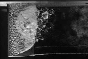
The physics and topology of a single cavity shedding cycle are complex and highly 3-D. The photographs in figure 15 show the development of the cavity for one cycle of the fundamental frequency, and the corresponding movie is included as supplementary movie 2. In the growth phase, the cavity has initially a crescent shape as shown in figure 15(a). This is due to faster growth at the root and tip than at midspan, leading to three-dimenional re-entrant flow. This jet reaches approximately  $x/c = 0.25$ (figure 15b) and is stable during the rest of the growth cycle. The cavity growth, then, at midspan is faster than at the root and tip, so the crescent shape disappears (figure 15b), and the cavity reaches the trailing edge. Now, a shockwave is triggered and moves upstream, partially condensing the cavity (in figure 15c, the downstream quarter of the cavity is opaque). For this flow configuration, the shockwave is the primary mechanism inducing cavity shedding, and, while a re-entrant jet is also present, it does not control the large-scale cavity breakup and shedding. The shockwave is focused as it travels upstream due to simultaneous shock fronts from the root and tip travelling towards the midspan of the hydrofoil. The shockwave reaches the leading edge and causes a detachment of the remaining cavity and subsequent advection downstream (figure 15d), which then rolls up into a large vapour cloud as shown in figure 15(a).

Figure 15. Photographs at one-quarter increments of the shedding cycle for the nuclei depleted condition. The cavitation number is 0.55i; (a)  $t'St_2=0$, (b) $t'St_2=1/4$, (c) $t'St_2=1/2$ and (d) $t'St_2=3/4$.
A space–time diagram of the same cycle is presented in figure 16 and is illustrative of the shedding phenomenon. The corresponding high-speed movie is included as supplementary movie 2. The vertical lines in figure 16 correspond to the time points for the photographs in figure 15. Flow is from the bottom to the top such that the trailing edge of the foil is at  $x/c=1$. The data was extracted from a spanwise position of $0.5b$. The upstream extent of the cavity is stable and varies only from $x/c=0.12$ to $x/c=0.14$. The blue highlighted region is the cavity growth phase and its motion along the hydrofoil. The green region indicates the upstream extent of the re-entrant jet flow, which is approximately constant at $x/c=0.25$. The cavity initially progresses towards the trailing edge at a velocity of $0.6U_\infty$. This velocity slows to $0.3U_\infty$ by the time it reaches the trailing edge. When this occurs, a condensation shockwave is triggered and travels upstream at a velocity of $-0.84U_\infty$. The shockwave propagation is in orange and its passage is marked by a small duration of translucency (black) where the cavity has been condensed. After the shockwave passage, the cloud is opaque indicating the presence of turbulent, bubbly flow characterised by much smaller length scales than the vaporous cloud. The red curve highlights the upstream extent of the cavity as it is shed from the hydrofoil and advects downstream. It is some 35 ms from when the cavity first reaches the trailing edge until it is advected downstream. In the annotated movie (supplementary movie 2), the horizontal line indicates the spanwise location of the space–time plot, and the coloured points correspond to the streamwise position of the various features as described above.

Figure 16. Space–time diagram of the shedding of a cloud cavity in a flow depleted of nuclei. The data is at the midspan of the hydrofoil ( $z/b = 0.5$) with flow from bottom to top. The purple lines indicate the time points of the snapshots in figure 15. The blue path traces the downstream extent of the cavity, the green is the re-entrant jet location, the orange is the passage of the shockwave and the red is the edge of the cavity as it is advected. The duration is 85 ms. Supplementary movie 2 corresponds to this same segment.
4. Shedding phenomena in nuclei-abundant flow
Consideration is now given to how the nuclei content influences the cavitation dynamics and resulting forces. Photographs of the cavitation behaviour in the shedding regime ( $0.60 \geq \sigma \geq 0.45$) with the addition of abundant nuclei are given in figure 17. The leading edge of the cavity (figure 18) changes from glassy cells downstream of a laminar boundary layer separation to discontinuous travelling bubble cavitation as there are an abundance of continually activated nuclei breaking up the leading edge. The boundary layer no longer separates so there are no leading edge cells associated with a continuous attached vapour cavity. The dominant spanwise length scales near the leading edge have increased and are associated with the size of bubble activations rather than the width of the leading edge cells. With reducing cavitation number, the cavity appearance does not change substantially beyond an increase in size. A cavitating trailing tip vortex is now visible, filled with discrete activating nuclei, which was not present in the depleted flow case.

Figure 17. Photographs of the cavity at various cavitation numbers. The free-stream is abundant with microbubbles.

Figure 18. Photographs of the leading edge of the cavity for the depleted and abundant populations. For the depleted case a series of glassy, spanwise cells indicate the presence of a laminar separation bubble. For the abundant case, this leading edge is broken up by many nuclei activations along the span, growing as separate bubbles. The cavitation number is constant at 0.55.
Figure 19 has the nuclei-abundant steady and unsteady force coefficients. The time-averaged lift is slightly lower in the nuclei abundant flow, attributable to the larger area that the cavity now forms over the planform. The drag force is similar to the depleted case. The unsteady fluctuations are slightly lower in the lift except for  $\sigma =0.6$, but the drag fluctuations are higher.

Figure 19. Steady (a) and unsteady (b) coefficients of lift (squares) and drag (triangles) in both the depleted (blue) and abundant (orange) seeding flow coefficients. The mean lift is reduced with the abundant seeding, but the unsteady component is relatively unaffected.
Although differences in forces between the two nucleation cases are not large, the cavity shedding is driven by different mechanisms. Considering the same flow conditions as in the previous section ( $\sigma =0.55$), but now with an abundant nuclei population, several salient changes may be noted. Firstly, a comparison of the spectrum of the lift force is given in figure 20. Besides the PSD, the magnitude of the CWT is also given, showing the main peaks to be $f_1$ and $f_2$, with the other harmonics evident in the PSD to be artefacts of the fast Fourier transform. The primary shedding mode is now $f_1$ (as will be shown in the following discussion), which is some 1.8 times slower than the shedding mode in the nuclei-depleted flow. The spatial distributions of the two modes are given in figure 21. The fundamental mode in figure 21(a) shows power across the entire area of the cavity downstream of $x/c=0.25$. The harmonic $f_2$ (figure 21b) shows a similar distribution indicating that this is the same mechanism but manifested at twice the frequency. This mode is associated with a second shockwave that occurs each cycle.

Figure 20. The PSD of the lift coefficient at a cavitation number of 0.55. The blue spectrum is with depleted water and the orange is with abundant nuclei. The CWT with abundant nuclei is given in the dotted line. The grey is the non-cavitating condition.

Figure 21. Spatial distribution of the PSD of the two most dominant frequencies for the nuclei-abundant case. The primary shedding mode is in (a) with the first harmonic in (b).
The time series of the lift coefficient and the corresponding space–time diagrams in figure 22 are plotted with the same time scale as figure 14, showing the slower shedding mechanism with a period of  $t'=6.5$ ( $St = {1}/{t'}=0.15$). The space–time diagrams beneath show the two shockwaves (oblique lines with negative gradients, as annotated in figure 24) of each cycle. The flow is much more 2-D as seen by the spanwise space–time in the bottom row. More details on each of these features are given below.

Figure 22. Time series (a) of the lift coefficient and space–time diagrams (b–d) from the high-speed movie. The space–time cavitation photographs are streamwise slices at  $z/b=0.3$ (b) and $z/b=0.7$ (c), and (d) is a spanwise slice at $x/c=0.8$. For the two streamwise space–time diagrams (b,c), the flow is from bottom to top. The flow is abundant with nuclei and the cavitation number is $\sigma = 0.55$. The duration of the sequence is 0.65 s. Here $T_1$ and $T_2$ refer to the primary and harmonic shedding periods, respectively.
A sequence of photographs showing one cycle of a cavity shedding event is given in figure 23, which is an excerpt of the movie available in supplementary movie 3. The cavitation number is 0.55, the same as that presented in figure 15, but now the shedding cycle is slower than the nuclei depleted case by a factor of 1.8. The shedding dynamics are now controlled by the passage of two consecutive shockwaves in each cycle. The first shockwave forms once the growing cavity reaches the trailing edge (between figures 23b and 23c). This shockwave propagates upstream (figure 23c) but loses strength and speed, stalling before reaching the cavity leading edge. Shortly after this, when another cavity packet reaches the trailing edge, a second shockwave forms that travels upstream with greater strength and velocity (figure 23d) causing large-scale condensation with subsequent near-2-D regrowth along the hydrofoil span (figure 23a). Due to the discontinuous nature of the cavity leading edge and the continuous supply of activated nuclei, the leading edge of the cavity is not condensed completely each shedding cycle as was the case for the nuclei-depleted case. Nuclei activated at the hydrofoil leading edge grow as they are advected downstream merging to form a contiguous cavity volume. Cavity growth is due to the volume of activated nuclei being greater than the condensing volume at the cavity trailing edge.

Figure 23. Photographs at one-quarter increments of the shedding cycle for the nuclei abundant condition. The cavitation number is 0.55; (a)  $t'St_1 = 0$, (b) $t'St_1 = 1/4$, (c) $t'St_1 = 1/2$ and (d) $t'St_1 = 3/4$.
A space–time diagram of the same cycle is given in figure 24 with corresponding annotated movie included in supplementary movie 4. The vertical lines correspond with the instances of the photographs in figure 23. There is no longer a clear cavity detachment line at the leading edge, but rather a series of oblique streaks which represent the activating microbubbles. These are advected at approximately the local velocity, which is measured as the gradient of these activations as  $1.23 U_\infty$. The blue region shows the growth of the cavity at approximately $0.25U_\infty$, less than half the growth-rate in the nuclei-depleted case. The green line marks the upstream reach of the re-entrant liquid jet. The orange lines are the two shockwaves. The first shockwave is the ‘lazy’ shock which is initiated when the cavity (blue) first reaches the trailing edge. The velocity of this shockwave is initially comparable to the depleted case at $-0.87U_\infty$, however, when the shockwave reaches $x/c = 0.4$, it slows to $-0.27U_\infty$. The second shockwave is faster, travelling at approximately $-U_\infty$ until $x/c=0.3$, from then it gradually slows to $-0.3U_\infty$. When this second shockwave reaches the leading edge, it extinguishes the cavity (with the exception of newly activating microbubbles) and the cycle is restarted.

Figure 24. Space–time diagram of the shedding of a cloud cavity in a nuclei abundant flow. The data is at the midspan of the hydrofoil ( $z/b = 0.5$) and flow is from bottom to top. The purple lines indicate the time points of the snapshots in figure 23. The blue path traces the downstream extent of the cavity, the green is the re-entrant jet location, the orange is the passage of the two shockwaves and the red is the edge of the cavity as it is advected. Note that the duration of 155 ms is a different time scale to that in figure 16. Supplementary movie 4 corresponds to this same segment.
The change in shedding behaviour with the additional nuclei is not limited to a single cavitation number. Figure 25 shows the PSD for all cavitation numbers with depleted water in blue and abundant in orange. The fundamental shedding mode for the abundant case is reduced to the low-frequency mode for all cavitation numbers investigated. The frequency of this is relatively independent of the cavitation number, which is comparable to the so-called Type I shedding mode observed by Smith et al. (Reference Smith, Venning, Pearce, Young and Brandner2020b) at low cavitation numbers.

Figure 25. The PSD of the lift coefficient as it varies with the cavitation number. The vertical offset is proportional to the cavitation number. The blue spectra represent the depleted data and the orange is the abundant.
5. Optimal nuclei content for minimal force fluctuations
The significant difference in shedding physics between the depleted and abundant nuclei populations raises the question of what occurs at intermediate populations. Photographs showing the influence of different nuclei concentrations are given in figure 26. A stainless steel hydrofoil was used for improved illumination in the photographs, and comparisons with the aluminium hydrofoil show no qualitative difference between the two models. In figure 26(a), there are no microbubbles injected (depleted), and figure 26(c) is the same abundant nuclei concentration described in the previous section. An intermediate concentration of the order of one microbubble per millilitre, referred to as ‘sparse’, is generated and the associated cavitation pattern is photographed in figure 26(b). This low concentration of microbubbles breaks up the continuous leading edge into smaller spanwise segments.

Figure 26. Photographs of the cavity appearance for the three concentrations of nuclei. All flow characteristics are identical between the photographs ( $\sigma =0.55$, $Re=1.4\times 10^{6}$) except the nuclei population.
The hydrofoil is more efficient with depleted seeding than with abundant. The mean forces are given in figure 27(a), showing no change in the forces with an increase in nuclei concentration (reduction in  $\sigma _{gen}$) until $\sigma _{gen} = 0.55$, where the production rate of the generators increase. Beyond this, there is a decrease in the lift force with increased concentration. The lift reduction is from 0.33 to 0.28, or 16 % between the depleted and abundant cases. For the sparse case at $\sigma _{gen} = 0.55$, there is no reduction in the lift. The time-averaged drag shows no measurable difference with concentration variation. The fluctuating drag coefficient (figure 27b) increases with nuclei concentration for seeding populations denser than the ‘sparse’ condition ( $\sigma _{gen} < 0.55$). The lift fluctuations indicate the extent of the shedding, with a similar value measured for both the sparse and abundant cases. Between these two conditions, however, there is a reduction in the shedding activity, reaching a minimum at $\sigma _{gen} = 0.5$.

Figure 27. Time-averaged (a) and fluctuating (b) force coefficients for various levels of microbubble seeding. The lift and drag are given by squares and triangles, respectively. The seeding density increases towards the left of the figures. The blue vertical line is the depleted case, the orange is the abundant and the green is the sparse. The free-stream cavitation number is 0.55.
The spectrogram in figure 28 shows the shedding mode changes as the nuclei concentration varies from depleted (top, blue) to abundant (bottom, orange) with the modes reducing from a three-mode system at the top (as described in § 3), to a dual-shockwave regime at the bottom (as described in § 4). Within a narrow-band of generator cavitation numbers near 0.55, there is a reduction in the strength of both shockwave-induced shedding modes. The individual spectrum is given in green in figure 29 and compared with the single-phase, depleted and abundant cases. With this sparse nuclei concentration, the occasional nucleus breaks up the leading edge, and the randomness in the spanwise size of the shed structures substantially reducing the predominance of any one shedding frequency.

Figure 28. Spectrogram of the lift coefficient for various generator cavitation numbers ( $\sigma _{gen}$). The seeding density increases downwards. The depleted, abundant and sparse injection cases are indicated by the blue, orange and green lines, respectively, corresponding to the colours in figure 29.

Figure 29. The PSD of the lift coefficient at a cavitation number of 0.55. The blue spectrum is with water depleted of nuclei, the orange is with abundant seeding, and the green is with the optimal, sparse seeding. The grey is the non-cavitating condition.
The time series for this ‘optimal’ case is given in figure 30 with the corresponding space–time diagrams given below. There are no dominant time scales evident over this sequence. The cavity growth is chaotic and cavity lengths prior to breakoff vary from quarter-chord to full-chord. The incoherence in these length scales leads to temporal incoherence and thus diminished spectral peaks. The mechanism for suppression of coherence is due to sparse nuclei activation at random spanwise locations such that the spanwise continuity of the shockwave is disrupted, hence limiting the global coherence of the cavity shedding. The corresponding movie is available as supplementary movie 5.

Figure 30. Time series (a) of the lift coefficient and space–time diagrams (b–d) from the high-speed movie. The space–time cavitation photographs are streamwise slices at  $z/b=0.3$ (b) and $z/b=0.7$ (c), and (d) is a spanwise slice at $x/c=0.8$. For the two streamwise space–time diagrams (b,c), the flow is from bottom to top. The flow is sparsely seeded with nuclei and the cavitation number is $\sigma = 0.55$. The duration of the sequence is 0.65 s.
To summarise the effect of nuclei content on the cavity shedding dynamics, three space–time diagrams are given in figure 31. The flow conditions are identical between the figures, except for the nuclei population. The change in relevant time scale (slowing down of the cavity shedding) is evident by the stretching in the horizontal direction. The coherence and repeatability of the shedding mechanism is clear for the depleted and abundant cases, and the lack thereof in the sparse case highlights how variable the cavity size, and therefore force fluctuations, are.

Figure 31. Comparison of streamwise space–time diagrams at  $z/b=0.5$ for the three seeding conditions at a cavitation number of 0.55. The flow is from bottom to top.
6. Conclusions
The dynamics of cloud cavitation about a hydrofoil have been shown to be affected by the free steam nuclei content for otherwise identical flow conditions. Simultaneous high-speed imaging and force measurements reveal the coupling between the cavitation behaviour and the generated forces. The mechanisms that lead to instability and cavity shedding vary according to the nuclei content of the water, which was varied from essentially no active free-stream nuclei to an abundant case with a high concentration of active nuclei. Nuclei control was achieved through injection of supersaturated water through cavitating nozzles in conjunction with bubble removal through gravity separation and dissolution throughout the tunnel circuit. For the nuclei-depleted case, a shedding cycle is made up of cavity growth until the cavity reaches the trailing edge, initiating upstream propagation of a condensing shockwave. This two-stage cycle repeats at a frequency of  $St=0.28$. While a re-entrant jet is ever-present, it is not the cause of the shedding instability. Two additional frequencies were present in the depleted case: a subharmonic and a harmonic mode. The CWT shows these modes to be generally exclusive of each other, and spectral decomposition shows them to be prevalent near the tip of the hydrofoil. The presence of abundant nuclei slows the dominant shedding frequency by a factor of 1.8 to $St = 0.15$. A harmonic mode exists due to the propagation of a secondary, ‘lazy’ shockwave which travels the length of the hydrofoil but causes only partial condensation. Following this preconditioning, the primary shockwave then condenses a much larger region of the cavity, after which there is regrowth to begin another shedding cycle. There is an intermediate seeding level which is optimal from the point of view of reducing the unsteady forces while maintaining hydrofoil lift generation. The activation of sporadic microbubbles (sparse seeding) breaks up the continuous leading edge of the attached cavity, reducing the coherence of large-scale shedding as revealed by space–time imaging and force measurements, with no loss in hydrofoil lifting efficiency. This suggests that there is the potential to reduce the level of unsteadiness induced by cloud cavitation about a lifting surface by the introduction of a controlled low level of microbubbles into the flow upstream of the device. This has significant implications for the enhanced operation of lifting surfaces and propulsion devices, particularly in off-design conditions.
Supplementary movies
Supplementary movies are available at https://doi.org/10.1017/jfm.2022.535.
Acknowledgements
The authors wish to acknowledge the technical support of Mr R. Wrigley and Mr S. Kent and the assistance of Dr D. Giosio and Dr S. Smith in acquiring the experimental data.
Funding
The authors appreciate the support of the Australian Defence Science and Technology Group (DSTG), the US Office of Naval Research (Dr K.-H. Kim, Program Officer) and ONR Global (Dr W.-M. Lin) through NICOP S&T grant no. N62909-15-1-2019.
Declaration of interests
The authors report no conflict of interest.


 Open access