


1. Introduction
Fluid in a narrow gap between elongated bodies can respond in resonance with incident waves at certain frequencies, yielding significant free surface motions – the so-called gap resonance. This is an interesting hydrodynamic phenomenon involving wave–structure interactions, body motions and fluid resonances in which both viscous and potential flow damping and nonlinearities all play a significant role. One practical application is an offloading operation between a floating liquefied natural gas facility and a liquefied natural gas carrier in a side-by-side configuration (Zhao et al. Reference Zhao, Milne, Efthymiou, Wolgamot, Draper, Taylor and Eatock Taylor2018a).
Early pioneering studies (Molin Reference Molin2001; Molin et al. Reference Molin, Remy, Kimmoun and Stassen2002; Sun, Eatock Taylor & Taylor Reference Sun, Eatock Taylor and Taylor2010) have demonstrated that gap resonances are standing waves in a gap, where the gap length is close to an integer multiple of half wavelengths for each standing wave (or gap mode). The gap resonances with different but closely spaced modal frequencies interfere in the gap, making the water free-surface motions rather complicated.
It is well established that the gap resonant mode shapes and frequencies can be estimated theoretically (e.g. Molin et al. Reference Molin, Remy, Kimmoun and Stassen2002, Reference Molin, Zhang, Huang and Remy2018) or numerically (e.g. Sun et al. Reference Sun, Eatock Taylor and Taylor2010), based on potential flow theory. However, the response amplitudes tend to be significantly overestimated by potential flow calculations. It is generally held that viscous damping needs to be considered, so as to achieve accurate prediction of response amplitudes. Many methods to improve the level of agreement between potential flow calculations and the results of physical experiments have been proposed, including rigid (Huijsmans, Pinkster & De Wilde Reference Huijsmans, Pinkster and De Wilde2001) or flexible lids at each (generalized) mode (Newman Reference Newman2001) and a dissipative damping term in the free-surface condition (Chen Reference Chen2005; Zhao et al. Reference Zhao, Milne, Efthymiou, Wolgamot, Draper, Taylor and Eatock Taylor2018a). A summary of other recent developments on gap resonances can be found, for example, in Zhao et al. (Reference Zhao, Wolgamot, Taylor and Eatock Taylor2017). The selection of the additional damping coefficient is generally empirical, requiring a better understanding of the viscous damping.
To account for viscous damping, in particular vortex shedding, Faltinsen & Timokha (Reference Faltinsen and Timokha2015) estimated the damping coefficient for sharp-edged boxes by combining the approximation of Molin (Reference Molin2001) and the pressure drop coefficient formula for a slatted screen. Considering both wall friction and flow separation, Tan et al. (Reference Tan, Lu, Tang, Cheng and Chen2019) reported a method to estimate associated damping coefficients using a series of model tests and empirical formulae. These damping coefficients were then implemented into a potential flow solver to match the results in Faltinsen & Timokha (Reference Faltinsen and Timokha2015). Allowing for body motions (in roll only), Milne et al. (Reference Milne, Kimmoun, Graham and Molin2022) investigated the vortex shedding dynamics at the sharp edges of a rectangular hull fixed in the vicinity of a vertical wall. A secondary separation was observed at the sharp edges, demonstrating the complexity of the gap flow. It is worth noting that these studies have focused on two-dimensional cases, while three-dimensional scenarios are rather more complicated.
Using a three-dimensional set-up, Ohkusu (Reference Ohkusu1976) showed an interesting phenomenon: the second-order sway drift force between two floating vessels could experience a sign change with gap width as a result of gap resonances; this led to slowly oscillating drift motions of the smaller vessel in regular wave excitations. Recent three-dimensional studies such as Molin et al. (Reference Molin, Remy, Camhi and Ledoux2009), Perić & Swan (Reference Perić and Swan2015) and Chua et al. (Reference Chua, de Mello, Nishimoto and Choo2019) conducted experimental and numerical modelling, with their focus on deriving regular wave response coefficients that are important for linear analysis. It is, however, also of practical interest to examine the nonlinear hydrodynamics, e.g. long swells (with periods  $\sim$14 s) exciting gap resonances ( $\sim$7 s) in offshore operations at sea. To investigate the gap behaviour in three dimensions, Zhao et al. (Reference Zhao, Wolgamot, Taylor and Eatock Taylor2017) conducted a comprehensive study for two fixed rectangular bodies with rounded corners, which is a pure diffraction problem. The viscous damping involved is shown to be compatible with Stokes-type laminar boundary layers at laboratory scale. Most strikingly, significant gap resonant responses can be excited through a nonlinear frequency-doubling process, e.g. the second harmonics are as significant as the linear responses. The spatio-temporal behaviour of gap resonances is explored in Zhao et al. (Reference Zhao, Taylor, Wolgamot, Molin and Eatock Taylor2020), again for fixed bodies. It remains unclear whether significant resonant responses can be excited nonlinearly when the bodies are freely floating, and, if so, how the gap resonances will behave.
In light of the above, the objectives here are to devise an experiment – using the same models as in the diffraction problem (Zhao et al. Reference Zhao, Wolgamot, Taylor and Eatock Taylor2017) – to investigate comprehensively the fluid resonant responses in a narrow gap and the associated dynamic motions of the floating body. Therefore, this study focuses on a coupled problem. To facilitate comparison and contrast, the gap resonance is excited by focused transient wave groups with broadside incidence, similar to that in the diffraction problem where two bodies are held fixed (Zhao et al. Reference Zhao, Wolgamot, Taylor and Eatock Taylor2017). The nonlinear hydrodynamics of body motions and gap resonances are analysed comprehensively, with interesting new phenomena unravelled.
This study is organised as follows. Following this Introduction, the experimental set-up and the wave generation in a wave basin are described in § 2. The linear and nonlinear harmonics of the gap surface responses are presented in § 3. We aim to compare and contrast these results to those obtained previously in a diffraction problem. A new gap mode is found to dominate the gap resonance in this coupled problem, whose mode shape is examined in § 3.5. Physical explanations are provided in § 3.6 for the observed hydrodynamic phenomena. In § 4, we show the linear and nonlinear harmonics of the body motions and the dynamics of the mooring lines connecting the two bodies. The super-harmonics of the body motions and the gap resonances show very similar shapes in time. The coupling processes between these are identified in § 5. Some important conclusions are presented in § 6. Finally, a semi-analytical model, reported in detail in Appendix B, is developed to shed further insight.
2. Wave basin experiments
2.1. Experimental set-up
The experiments were carried out in the Deepwater Wave Basin at Shanghai Jiao Tong University. This wave basin is 50 m long and 40 m wide, and the water depth can be adjusted from 0 to 10 m using an artificial bottom; here, the depth was set to 7 m.
The experiment represents a 1 : 60 scaled version of a simplified geometry, with gap width around 4 m and gap length 200 m at full scale. As shown in figure 1, two rectangular bodies with identical wet surface geometry were used in the experiments. The bodies are prismatic and 3.333 m long at model scale. In cross-section they are 0.767 m wide with round corners at both bilges, each with radius 0.083 m running along the length. Both bodies are immersed such that the undisturbed draught is 0.185 m, leading to a 0.102 m high vertical surface below the mean water surface. One of the bodies is 0.425 m high, and the other is 0.6 m. Details of the inertia parameters for the floating body are given in table 1.
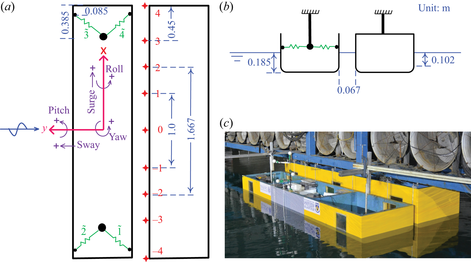
Figure 1. Sketch of the two bodies in side-by-side configuration, with one floating and the other fixed: (a) plan view, (b) side view, and (c) a snapshot of the two body hulls (yellow) in a wave basin. The fixed body is rigidly connected with the gantry (blue), and the floating one is moored by horizontal spring lines (green). The ‘ $+$’ symbols in (a) demonstrate the positive direction of the body motions, and the red cross symbols indicate the locations of wave gauges that are stick to the fixed body. A specific pre-tension is applied to each of the four spring lines to avoid slackness in the testing, and the measured force data reflect the instantaneous line tensions with the pre-tensions removed.
Table 1. Particulars of the floating body model and the mooring lines. Here, CoG stands for the centre of gravity. All the parameters are given in laboratory scale. The fixed body model has the same hull geometry as the floating one.

The two bodies are arranged in a side-by-side configuration, with the taller one being mounted rigidly on a gantry in the wave basin. One body is fixed, and the other is floating. The gantry is very robust, providing enough stiffness to prevent vibration of the body models at frequencies of interest in this study. The floating body is connected to the fixed one via four identical soft spring lines (marked in green in figure 1a), forming a narrow gap of width 0.067 m in calm water between the two bodies. The positions and stiffnesses of the soft spring lines have been designed to represent realistic scenarios, e.g. to mimic the natural frequencies of surge, sway and yaw motions. The inertia parameters are also selected to represent typical values in realistic operations. Free decay testing was conducted in otherwise calm water, with the purpose of checking the experimental set-up. To facilitate the analysis, the measured natural frequencies of the floating body motions are listed in table 2.
Table 2. Natural frequencies (or periods) of the floating body determined through decay testing in otherwise calm water. The decay testing was performed with the floating body in side-by-side configuration next to the fixed one. The symbols  $\zeta$ and $f$ denote the motion modes and natural frequencies of surge, sway, heave, roll, pitch and yaw, respectively. The corresponding natural periods ( $T$) at full scale are also given to facilitate reading.

Standard resistance-type wire gauges – marked by the red crosses in figure 1 – are deployed along the gap length, to measure the surface elevations. The mid-point of the gap was 20 m away from the wave paddles and 20 m from the side walls of the wave basin. As shown in figure 1(a), there are nine wave gauges: 1 and  $-1$, 2 and $-2$, 3 and $-3$, 4 and $-4$ are symmetric in pairs about the gap centre, and 0 is central in the gap. The wave gauges have a measurement error less than 1 mm. The reliability of these wave gauges has been demonstrated in the Appendix of Zhao et al. (Reference Zhao, Wolgamot, Taylor and Eatock Taylor2017), and thus is not repeated here.
A Qualisys optical motion tracking system was employed, together with four passive optical balls (white balls in figure 1c) defining a rigid body, to measure the six-degrees-of-freedom motions of the floating body. The directions of the body motions are defined in figure 1(a), with positive heave being upwards. Load cells were fixed to each spring mooring line, to measure their force in the experiment. Details of the floating box and the mooring lines are given in table 1. The four horizontally deployed mooring lines were set at the same height as the vertical centre of gravity, avoiding linear coupling effects (in the stiffness matrix) between the horizontal and roll motions of the floating body.
2.2. Undisturbed incident wave
To facilitate comparison to our previous tests with the bodies held fixed, transient wave groups similar to those in Zhao et al. (Reference Zhao, Wolgamot, Taylor and Eatock Taylor2017) are generated to excite the body motions and the gap responses. In the wave generation, a large wave crest occurs at the focus position and time  $(x_0,t_0)$ with phase $\psi =0$. The shape of a unidirectional transient wave group is given by
 \begin{equation} \eta(x,t)=\frac{\alpha}{\sigma^{2}}\sum_{n=1}^{N}S(f_n)\,{\rm \Delta}{f} \operatorname{Re}[\exp({-{\rm i}k_n(x-x_0)+{\rm i}{2{\rm \pi}\,f_n}(t-t_0)+\psi})], \end{equation}
where  $\alpha$ corresponds to the expected maximum free surface elevation in a given sea state, $k_n$ and $f_n$ are the wavenumber and frequency of the spectral component, and the variance is $\sigma ^{2}={\sum _{n=1}^{N}}{S(f_n)\,{\rm \Delta} {f}}$.
In this study, the focus position of the transient wave group was set at  $x_0=20$ m from the equilibrium position of the wave paddles, which is also the location of the centre of the gap. In the experiments, waves approach the gap laterally as shown in figure 1 (broadside to the floating body, so beam seas). The underlying spectrum is Gaussian, given by
 \begin{equation} S(f)=\frac{H_s^{2}}{16}\,\frac{1}{\sqrt{2{\rm \pi}\delta^{2}}}\exp\left(-\frac{(f-f_p)^{2}}{2\delta^{2}}\right), \end{equation}
where  $H_s$ refers to the significant wave height, $f_p$ is the peak frequency of the spectrum, and $\delta =0.0775$ Hz is the (lab scale) shape parameter of the Gaussian spectrum, in which the focused wave group is assumed to occur.
In each set of the experiments, we run the same paddle signal four times, but with each input Fourier component being phase ( $\psi$) shifted at each run. This generates a set of four wave series, i.e. nominally crest-focused (0 $^{\circ }$), up-crossing (90 $^{\circ }$), trough-focused (180 $^{\circ }$) and down-crossing (270 $^{\circ }$), all with the same spectral shape as shown in figure 2.
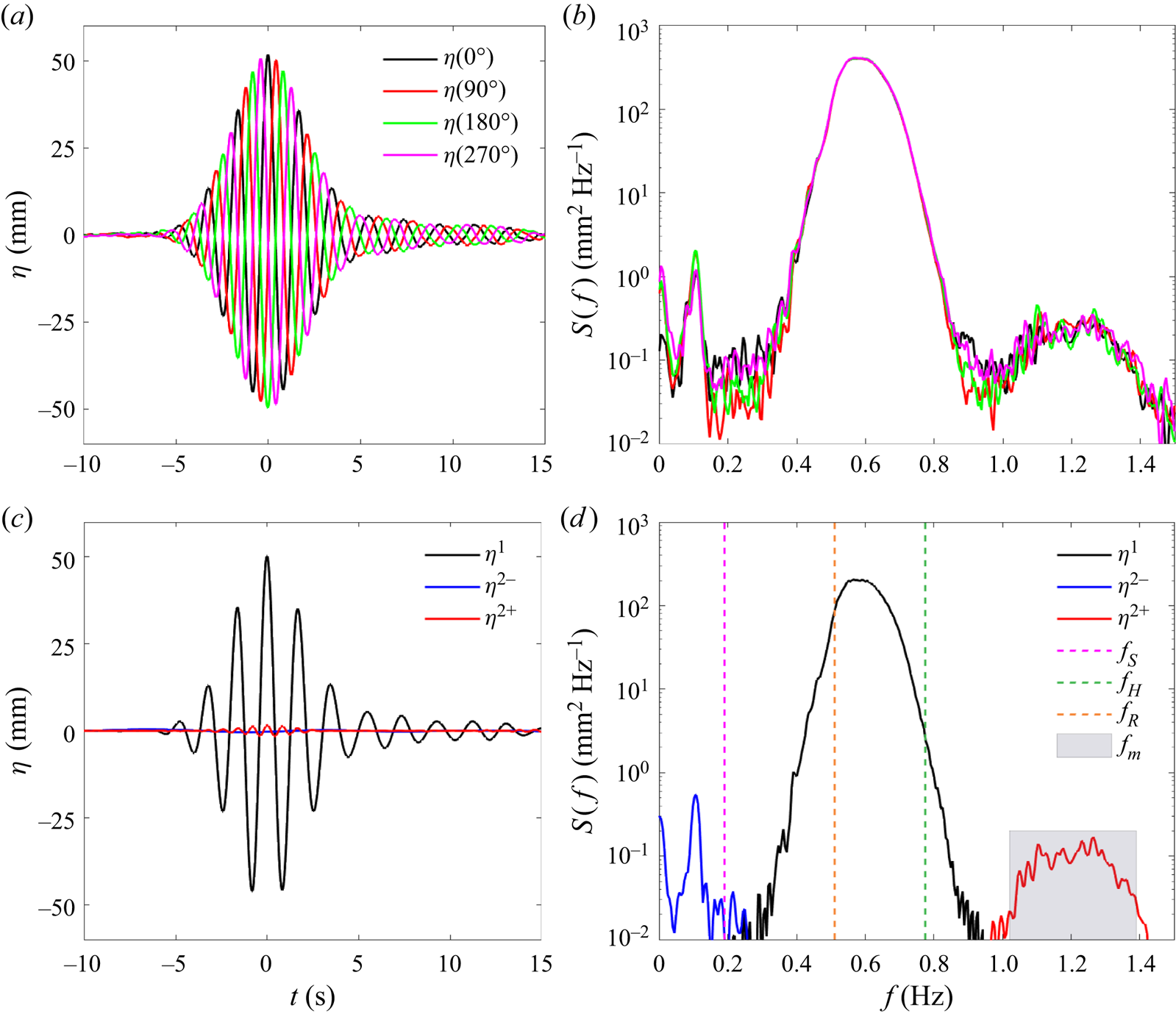
Figure 2. Undisturbed incident wave ( $\eta$) measured at the centre of the gap in the absence of the models: (a) time history of the measured data; (b) the corresponding spectra on a log scale; (c) time history of harmonic components; and (d) the corresponding spectra. The focal time of the undisturbed incident wave group is marked as $t=0$ s in (a,c). The superscripts 1, $2-$, and $2+$ in (c,d) refer to the linear, second-order difference and sum frequency harmonics, respectively. The vertical dashed lines in (d) indicate the natural frequencies of sway ( $\,f_{S}$), heave ( $\,f_{H}$) and roll ( $\,f_{R}$) motions of the floating body, and the shaded area covers the frequency range of the gap resonant modes that are of interest in this study. The first translational basin sloshing mode has frequency 0.107 Hz, where the blue curve in (d) peaks.
The four-phase wave signals are then combined to extract the first four harmonics, i.e.  $\eta ^{1}$, $\eta ^{2+}$, $\eta ^{3+}$ and $\eta ^{4+}$, referring to the terms with frequencies around $f_p$, $2f_p$, $3f_p$ and $4f_p$, respectively. The extracted harmonics are then associated with the Stokes-type expansion for nonlinear waves. For the sake of space, we do not repeat the four-phase decomposition theory here, but details can be found in Fitzgerald et al. (Reference Fitzgerald, Taylor, Eatock Taylor, Grice and Zang2014) or Zhao et al. (Reference Zhao, Wolgamot, Taylor and Eatock Taylor2017). As noted in Zhao et al. (Reference Zhao, Wolgamot, Taylor and Eatock Taylor2017), the second-order difference frequency term ( $\eta ^{2-}$) is embedded with the fourth harmonic signal, which can be extracted through digital filtering. We stress that we look at the harmonics in terms of wave frequency, which should be distinguished from the order of the Stokes-type expansion in terms of nonlinearity (powers of the wave steepness).
The incident waves here are observed to be dominated by the linear component, with sub-harmonics (i.e. second-order difference frequency term) and super-harmonics (i.e. second-order sum frequency term) being very small, and higher harmonics being invisible. Therefore, only the first two harmonics are plotted in figure 2(c). The (nominal) maximum amplitude of the linear component of the wave group is  $\alpha =50$ mm, as shown in figure 2(c). It is worth noting that the spectra have been plotted with a logarithmic vertical scale to better demonstrate the nonlinear components.
The peak frequency of the undisturbed incident waves in this study is designed to equal half that of the  $m=3$ gap mode, i.e. $f_p=0.5f_{m=3}$, so as to excite the gap resonance through nonlinear forcing. As shown in table 2, the natural frequencies of the low-frequency motion modes (surge, sway and yaw) have been designed to avoid basin sloshing modes, while being maintained close to realistic values for a 1 : 60 scaled model. In the beam sea excitations, surge (along the long axis of the body), pitch and yaw motion responses are negligible, as they should be due to the symmetry of the model set-up and the wave approach direction. One can see from the frequency alignment in figure 2(d) that heave and roll motions of the floating body could be excited linearly by incident waves, while there is no linear input wave energy around the frequencies of the gap resonances and the sway motions of the floating body. The latter can be driven only through nonlinear wave–structure interactions in this experimental set-up.
3. Spatio-temporal structure of gap resonance
The transient wave groups described in § 2.2 are generated to excite the gap resonances and the body motions for the experimental set-up shown in figure 1. The experiments, in terms of the water surface elevations, body motions and mooring forces, show extremely good repeatability. Details are demonstrated in Appendix A.
3.1. Symmetry of the experimental set-up
In the experiments, the unidirectional waves approach the floating body propagating perpendicular to the gap length. Therefore, the gap surface elevations measured by the wave gauge pairs at the symmetric locations, e.g. wave gauge pair 1 and  $-1$, should show identical results.
To demonstrate the quality of the experimental set-up, the time series of gap surface elevations (denoted as  $\varphi$) measured by the nine wave gauges are plotted in figure 3. To facilitate the analysis, the incident wave time series ( $\eta$) are also shown. One can see that strong gap surface elevations are driven in the excitation stage (e.g. from $t=-5$ to $t=5$ s). After the incident wave has passed, i.e. from $t=5$ s onwards, the fluid in the gap oscillates at higher frequency and decays slowly with a beating pattern. Wave gauges 4 and $-4$ are located at the ends of the gap, which are close to nodes of the gap modes, and thus show much weaker responses compared to those inside the gap.

Figure 3. Undisturbed incident waves ( $\eta _{tot}$) and the gap responses ( $\varphi _{tot}$) at different locations along the gap. The superscript ‘ ${tot}$’ refers to the total measured signal, and each numerical subscript represents the wave gauge label. Here, $t=0$ refers to the focal time of the undisturbed incident wave group. Note the different vertical axis scalings for the incident waves and the gap responses.
The wave gauge pairs, i.e. 1 and  $-$1, 2 and $-$2, 3 and $-$3, and 4 and $-$4, are deployed symmetrically with respect to the centre of the gap. As shown in figure 3, the measured data at the symmetric locations agree well in general, demonstrating the good symmetry in the experimental set-up. The slight difference between wave gauges 2 and $-$2, 3 and $-$3, could be associated with the tiny surge (with amplitude $\sim$2 mm) and pitch (with amplitude $\sim$0.35 $^{\circ }$) motions of the floating body. It is worth reiterating that the directions of the floating body motions have been defined in figure 1.
3.2. Harmonics of gap resonance – linear damping in nonlinear processes
To examine the nonlinear physics in the excitation of gap resonances, the harmonics of the measured signal in § 3.1 are extracted based on the four-phase decomposition method mentioned in § 2.2. As demonstrated in figure 3, the maximum gap surface responses (98 mm) occur at one- and three-quarters along the gap length, rather than at the centre (83 mm). Therefore, the measured data at one-quarter of the gap length are shown in this section as representative.
The first four harmonics of the gap responses ( $\varphi ^{1}$, $\varphi ^{2+}$, $\varphi ^{3+}$ and $\varphi ^{4+}$) are shown in figure 4, together with the first two harmonics of the incident waves. To demonstrate the nature of the various processes, the experiment was repeated with incident waves of smaller amplitude. The results yielded in the smaller wave test are given in figure 4, with the first, second, third and fourth harmonics being scaled up by $\mu \ (=1.4)$, $\mu ^{2}$, $\mu ^{3}$ and $\mu ^{4}$, respectively, where $1/\mu$ is the scaling factor applied to the paddle signals for the scaled groups.

Figure 4. Harmonics of the incident waves and the corresponding gap responses at one-quarter (wave gauge 2) of the gap length. The black dotted curves (denoted with subscript ‘ ${s}$’) are from the repeated run with a smaller amplitude of incident wave being scaled down by $\mu =1.4$. The superscripts ‘ $1$’, ‘ $2+$’, ‘ $3+$’ and ‘ $4+$’ refer to the linear, second, third and fourth harmonic components, respectively.
As shown in figure 4, the incident waves  $\eta$ – both the linear and the small second harmonics – agree very well between the two sets of experiments, indicating the quality of the wave generation. The gap responses are shown to be dominated by the first two harmonics, whereas the third and fourth harmonics are visible but small. It is of practical importance to note that the second harmonic $\varphi ^{2+}$ is even larger than the linear component $\varphi ^{1}$.
It is striking to see that these two sets of experimental results agree remarkably well, up to the third harmonics. The agreement of the fourth harmonics is less satisfactory, which is not surprising given that the magnitude of the fourth harmonic in the smaller wave test is tiny, i.e.  $\varphi ^{4+}_{s}=2.5/\mu ^{4}\approx 0.6$ mm.
The scaling between the two sets of experimental results in figure 4 confirms that the significant gap responses are driven through nonlinear processes with a quadratic, cubic and quartic dependency on wave amplitude, for  $\varphi ^{2+}$, $\varphi ^{3+}$ and $\varphi ^{4+}$, respectively. Further, such good scaling between the two sets of experiments can be possible only when the damping involved has a linear form. Therefore, the viscous damping of the gap responses must have a linear form in the range of amplitudes tested. This is consistent with the observation in the fixed body case – a pure diffraction problem (Zhao et al. Reference Zhao, Wolgamot, Taylor and Eatock Taylor2017). The damping is discussed further in § 5.
3.3. Gap resonance: diffraction problem versus coupled problem
In this subsection, we compare and contrast the gap resonances from the coupled problem (allowing free body motions) as shown in figure 1, and those from the diffraction problem (with both bodies held fixed) as reported in Zhao et al. (Reference Zhao, Wolgamot, Taylor and Eatock Taylor2017).
Figure 5 shows the time series of the undisturbed incident waves and the corresponding gap responses at the centre of the gap, where the maximum occurs for the diffraction problem. The undisturbed incident waves in the two cases have identical amplitudes, but slightly different frequency components. For instance, both waves are generated based on a Gaussian spectrum, but with the spectral peak frequency  $f_p=0.5f_{m=3}=0.57$ Hz for the coupled problem in this study, and $f_p=0.5f_{m=1}=0.51$ Hz for the diffraction problem in Zhao et al. (Reference Zhao, Wolgamot, Taylor and Eatock Taylor2017). As demonstrated in figure 5(b), the time series of the gap responses show considerable frequency variation across the entire signal: from frequencies similar to those of the incident waves (as a result of forced motions by incident waves), to those of the (freely-decaying) gap resonances. The most striking observation is that the gap surface responses $\varphi ^{tot}$ in the coupled problem are significantly larger, i.e. twice as large as those in the fixed body case ( $\varphi ^{{tot}}_{d}$).

Figure 5. Incident waves and gap responses at the centre (wave gauge 0) of the gap from the coupled problem in this study (black solid curves) and the diffraction problem reported in Zhao et al. (Reference Zhao, Wolgamot, Taylor and Eatock Taylor2017) (red dotted curves). The superscripts ‘ ${tot}$’, ‘ $1$’ and ‘ $2+$’ refer to the total signal, the linear and second harmonics, respectively. The subscript ‘ ${d}$’ indicates the diffraction problem with two bodies held fixed. The symbols $\hat {\varphi }^{1}_d$ and $\hat {\varphi }^{2+}_d$ (solid green curves) represent the estimated gap responses for the diffraction problem, but with the same incident wave as for the coupled experiment.
To better demonstrate the response difference between floating and fixed body cases, we examine their harmonic components. Based on the four-phase decomposition method mentioned in § 2.2, we separate the first four response harmonics  $\varphi ^{1}$, $\varphi ^{2+}$, $\varphi ^{3+}$ and $\varphi ^{4+}$. Here we show the gap resonance signal only to the second harmonics, as the higher harmonics are negligible. As shown in figures 5(c,d), the (non-resonant) linear gap response in the coupled problem (solid black curve) is twice as large as that for the diffraction problem (red dotted curve), and the (resonant) second harmonic in the former case is also much larger than that in the latter case.
To eliminate the possible effect of the slightly different peak frequencies in the incident waves, we calculate the gap responses for the fixed body case, based on the same incident waves – the solid black curve  $\eta ^{1}$ in figure 5(a) – as in the floating case. The numerically calculated linear and second harmonics of the gap responses (solid green curves) are given in figures 5(c,d), respectively. These calculations are based on transfer functions derived from the experimental data, rather than potential flow modelling, which ignores viscous damping. Deriving the linear transfer function from the experiments is straightforward, while the quadratic transfer function is obtained using the ‘flat QTF’ approximation that has been demonstrated in Zhao et al. (Reference Zhao, Taylor, Wolgamot and Eatock Taylor2021b). The calculated linear and second harmonics (solid green curves) are similar to those given in the red dotted curves. This is not surprising, as the incident waves differ only slightly.
In addition to the centre, it is also of great interest to examine the responses at one-quarter (or three-quarters) of the gap, where the maximum response occurs for the coupled problem. Figure 6 shows the total response signal at one-quarter of the gap for both the coupled problem and the pure diffraction problem, as well as the decomposed harmonic components. The incident waves, the same as in figure 5(a), are not shown here to avoid repetition. It is striking to see that the second harmonic of the gap response ( $\varphi ^{2+}$) is much larger in the floating case, e.g. three times as large as that for the fixed case. The $\varphi ^{2+}$ signal seems to be dominated by a particular gap mode, as the time series does not show an obvious beating pattern. The structure of the gap modes is examined in detail in the following subsections.

Figure 6. Similar to figure 5, but for the position of wave gauge 2, i.e. at one-quarter of the gap.
3.4. Structure of gap resonant responses in frequency space
Previous sections have been focused on the time series of the gap responses. This section investigates their spectral structures, to identify the resonant modes involved in these processes.
Spectral analysis is conducted for each of the gap resonance harmonics, and the results are shown in figure 7(a) for the signal measured at the centre of the gap, and in figure 7(b) at one-quarter along the gap length. The linear response components – concentrating in the frequencies 0.3–0.8 Hz – show similar spectral structure, for both the pure diffraction problem (red dotted curves) and the coupled problem (black dotted curves), albeit with much larger amplitude in the latter case. The spectral structure is rather smooth over the frequencies 0.3–0.8 Hz, because they are far away from the gap resonance frequencies, and the corresponding transfer functions do not vary significantly with frequency (see figure 4 in Zhao, Taylor & Wolgamot Reference Zhao, Taylor and Wolgamot2021a).

Figure 7. Amplitude spectra of the gap response harmonics for the coupled problem and the diffraction problem: (a) at the centre, and (b) at one-quarter of the gap length. The dotted curves are for the linear components, and the solid for the second harmonics. The vertical dashed lines indicate the frequencies of the gap resonant modes.
The comparison of the second harmonics (solid curves), around the gap mode frequencies, is more interesting. At the centre of the gap as shown in figure 7(a), the large peak associated with the  $m=1$ gap resonant mode in the diffraction problem becomes indiscernible in the coupled problem where body motions are allowed for. In contrast, the $m=3$ gap resonant mode appears to be amplified significantly in the coupled problem. This is consistent with the experimental observation in Chua et al. (Reference Chua, de Mello, Nishimoto and Choo2019) where both head and beam sea conditions are considered focusing on linear excitations. Here, the $m=1$ mode is shown to disappear even in complicated nonlinear wave–structure interactions. It is worth noting that the numerical simulations in Sun et al. (Reference Sun, Eatock Taylor and Taylor2010) with different vessel geometries also suggest the cancellation of the $m=1$ gap mode for the coupled problem, though it was not stated explicitly. Physical explanations of the disappearance of the $m=1$ gap mode are given in detail in § 3.6.
More striking is the behaviour observed at one-quarter along the gap length, as shown in figure 7(b). It clearly shows a significantly enhanced response peak in the coupled problem, which does not appear in the diffraction problem. The responses in the coupled problem are dominated by a gap resonant mode whose frequency lies between the  $m=3$ and $m=5$ gap modes. This resonant mode is new – it was not observed in the diffraction problem – and can only be a symmetric mode, given the good symmetry of the experimental set-up demonstrated in figure 3.
3.5. Mode shapes of the gap resonances
To better understand the structure of the new resonant mode appearing in the coupled problem, we derive the mode shapes from the experiment, as well as the numerical calculations based on linear potential flow theory.
Cross-spectral analysis is conducted across the nine wave gauges through  $S_{xy}(f)={\int _{{-\infty }}^{\infty }}{R_{xy}(\tau )\exp ({-\mathrm {i}{2{{\rm \pi} }f}\tau })\,{{\rm d}}\tau }$, where $R_{xy}(\tau )$ is the cross-correlation between the variables $x$ and $y$. The cross-spectral analysis yields the relative phase and amplitude information of the surface elevation at each wave gauge, which is used to construct the mode shapes. Details of the cross-spectral analysis can be found in Zhao et al. (Reference Zhao, Wolgamot, Taylor and Eatock Taylor2017). These mode shapes are then normalised and compared with those from linear potential flow calculations based on HydroSTAR.
As noted in the preceding subsection, the  $m=1$ mode, with half a wavelength along the gap, dominates in the diffraction problem but disappears in the coupled problem. Thus we show only the mode shapes of the first few gap resonances appearing in the coupled problem in figure 8. An interesting gap mode is observed, which features two half-wavelengths and dual peaks (in phase) at one- and three-quarters along the gap length. This double-humped ‘camel-back’ mode is new, and marked as $m=|2|$, as its mode shape resembles the modulus of the (antisymmetric) $m=2$ mode shape. It has a small non-zero value at the gap centre, whereas a $m=2$ mode would show a node. This new gap resonant mode shows how the maximum surface elevation, as demonstrated in figure 3, occurs at points close to one- and three-quarters along the gap length.

Figure 8. Mode shapes along the gap under broadside wave excitations for the coupled problem – a floating body in the vicinity of a fixed body. Here,  $x$ refers to the distance away from the mid-ship point, and the amplitudes have been normalised by their maxima. The dashed curves refer to the linear potential flow calculations, and the hollow dots denote the experimental data. The $m=1$ resonant mode disappears in the coupled problem here. The ‘camel-back’ resonant mode is new and was not observed in the pure diffraction problem.
3.6. Physics associated with the gap resonant modes
When going from the diffraction problem to the coupled problem, i.e. allowing for free body motions, the analysis above has demonstrated some interesting phenomena: the disappearance of the  $m=1$ resonant mode and the appearance of a new mode with a ‘camel-back’ shape. The newly observed ‘camel-back’ mode dominates the gap responses in the coupled problem.
To explore the physics behind such phenomena, we look into the linear frequency domain potential  $\phi$, which is given conventionally as
 \begin{equation} \phi(x,y,z,\omega)=\phi_D(x,y,z,\omega)+ \sum_{\mu=1}^{6}v_\mu(\omega)\,\phi_\mu(x,y,z,\omega), \end{equation}
where  $\phi _D$ refers to the diffraction potential (including the incident wave potential), $\phi _\mu$ is the radiation potential due to body motions in the $\mu$th mode with unit velocity, and $v_\mu$ is the body velocity in the $\mu$th mode due to incident waves with unit amplitude.
When these potentials and body velocities are regarded as functions of complex frequency, a resonance corresponds to a pole in the complex-frequency domain that lies close to the real frequency axis. It has been demonstrated (McIver Reference McIver2005) that a pole in the radiation potential gives no corresponding pole in the potential for the coupled problem. In general, each pole in the radiation potential has a corresponding pole in the diffraction potential, due to the connection between the two solutions. The corresponding poles in the radiation and diffraction potentials are cancelled out in the solution of  $\phi$ to the coupled problem. As a result, the resonant modes (e.g. $m=1$ resonant mode) that correspond to poles in the radiation or diffraction problem, sometimes called ‘sloshing resonances’, disappear in the coupled problem. The fluid motion will then be dominated by any nearby resonances (‘motion resonances’) that arise from the poles of the body velocity $\boldsymbol {v}$.
These motion resonances are the non-trivial solutions (in the complex-frequency plane) of the homogeneous equation of motion, and a pole in the body velocity  $\boldsymbol {v}$ gives a pole in the potential $\phi$ for the coupled problem. Additional poles (beyond those due simply to the mass and spring) in $\boldsymbol {v}$ arise due to the poles in the radiation potentials, but the frequencies are shifted due to the vessel mass and stiffness properties. Hence the solution for the coupled problem occurs at a different complex frequency to the poles in the radiation potentials. In practice, a ‘motion resonance’ often occurs at a frequency close to each ‘sloshing resonance’ so that the phenomenon described here is observed as a small shift of the resonance frequencies (McIver Reference McIver2005), when going from a diffraction/radiation problem to a coupled problem.
The higher gap resonance modes also have poles in the radiation potential, though they may be further away from the real axis in the complex-frequency plane. By analogy, these poles will not yield corresponding poles in the coupled potential, but there should be associated poles in the velocity vector  $\boldsymbol {v}$. The frequencies of the peak elevation in the coupled problem and those in the radiation problem are expected to be slightly different, and gradually the differences get smaller for higher modes.
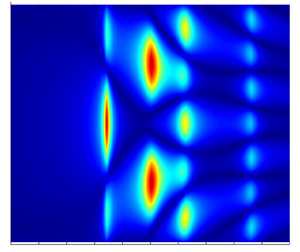
To ‘visualise’ these effects, we run linear potential flow calculations using HydroSTAR for the same configuration as in the experiment. The stiffnesses of the horizontal mooring lines are accounted for. Viscous damping effects have been ignored, as the aim here is to understand the mechanism involved rather than to seek the exact amplitude of the response. Figure 9 shows the modulus of the linear transfer functions for the surface elevations along the gap length, with figure 9(a) showing the diffraction field  $\phi _D$, figure 9(b) the radiated field $\sum _{\mu =1}^{6}v_\mu \phi _\mu$, and figure 9(c) the total field $\phi$. The numerical simulations clearly demonstrate that the $m=1$ resonant mode appears in both the diffraction and radiation fields, and is cancelled out in the coupled problem. Here, we emphasise that the disappearance of the $m=1$ gap mode is general for a coupled problem, which is also clear from the complex resonance analysis of McIver (Reference McIver2005).

Figure 9. Modulus of transfer functions for surface elevations along the gap with broadside wave incidence based on linear potential flow calculations: (a) the diffraction field per unit wave amplitude  $\phi _D$; (b) the radiated field per unit wave amplitude, i.e. $\sum _{\mu =1}^{6}v_\mu \phi _\mu$; and (c) the total field per unit wave amplitude $\phi$. The vertical axis $x$ has the same meaning as in figure 8. Viscous damping was ignored in the calculations, but stiffness of the horizontal mooring lines was taken into account. The $m=1$ mode, appearing in both diffraction and radiation fields, is cancelled out in the total wave field. A ‘camel-back’ mode appears and dominates in the radiation and total fields.
To identify the dominating factor that causes the phenomena above, we look into the radiation field and the body velocity corresponding to each degree-of-freedom motion. Only the sway, heave and roll motions are of interest here, as the remainder are not excited due to symmetry. Roll motions are observed to have radiation and velocity structures similar to those in the sway motion, but their amplitudes are much smaller. To save space, we show only the radiation field and the body velocity for sway and heave motions in figure 10.

Figure 10. Similar to figure 9, but only for sway (upper half) and heave (lower half) motions, with (a) the radiation field  $\phi _\mu$ due to a body motion with unit velocity in the $\mu$th mode, (b) the body velocity $v_\mu$ in the $\mu$th mode per unit wave amplitude, and (c) the product $v_\mu \phi _\mu$. The body velocity does not vary along the gap length, thus simple curve plots are sufficient. Note the different vertical scales in (b), which refer to the body velocity.
The results in figure 10 seem to suggest that both sway and heave play an important role in the cancellation of the  $m=1$ resonant mode, whereas it is the sway motion that is primarily responsible for the new ‘camel-back’ resonant mode. There is nothing special in the sway radiation field $\phi _2$ (at $f=1.2$ Hz) as shown in figure 10(a), but the strong resonant peak at this frequency in the velocity field $v_2$ (in figure 10b) clearly yields a large product $v_2\phi _2$ in figure 10(c). The heave motion seems to contribute in a similar way, but with a greatly weakened effect. Thus the ‘camel-back’ mode is coupled mainly with the resonance of the body velocity in sway, a ‘motion resonance’. Variation in the mooring stiffness will lead to changes in the body velocity property. When the stiffness becomes sufficiently large, tending to infinity, the full analysis tends to the simple diffraction problem where the ‘motion resonance’ mode disappears.
Focusing on the sway mode only, a semi-analytical model is developed to calculate the fluid motion in the gap between a floating body and a fixed body. The model confirms that a variety of spatial structures in the gap are possible at frequencies away from the sloshing resonances, which could then be amplified by a motion resonance, given appropriate mass and stiffness properties. Details of the analysis and the semi-analytical model are given in Appendix B.
This section has been focused on linear potential flow analysis, which well explains the interesting phenomena when going from a diffraction problem to a coupled problem. It is worth emphasising that the occurrence of such phenomena in the experiments is striking, as the gap resonances are driven through nonlinear wave–structure interactions.
4. Linear and higher harmonics of body motions and mooring load
In beam sea excitations, there is little response in surge, pitch and yaw due to the symmetry of the experimental set-up. Therefore, the focus here is on sway, heave and roll motions, together with the load acting on the mooring system.
4.1. Linear and nonlinear roll motions
The spectral peak frequency (0.57 Hz) of the incident wave equals half that of the  $m=3$ gap mode, which is near the natural frequency (0.51 Hz) of the roll motion for the floating body. As a result, significant roll motions are expected to be driven through linear wave excitations.
As shown in figure 11(a), the roll motions feature a very slow decaying process, after the excitation of the transient wave groups that exist for only a few seconds (up to  $t=5$ s, as shown in figure 2). This is not surprising as the floating body has a round bilge, leading to low damping in roll in terms of both viscous stresses acting on the hull and weak wave radiation.

Figure 11. Time histories and spectra of the first and higher harmonics of the roll motion. The subscript ‘ $R$’ refers to the roll motion. The superscripts ‘ ${tot}$’, ‘ $1$’, ‘ $2-$’ and ‘ $2+$’ refer to the total signal, the linear, the second-order difference frequency and the sum frequency components, respectively. The subscript ‘ $m$’ represents the gap modes. Note the logarithmic scale of the vertical axis for the power spectra in (c).
The four-phase decomposition method has already been shown to work for body motions (Zhao et al. Reference Zhao, Taylor, Wolgamot and Eatock Taylor2018b), although it was originally developed for free-surface waves. Here, the first four harmonics of the roll motions are extracted using this decomposition methodology, as for the undisturbed incident waves in § 2.2. It is worth noting that the measured time histories are contaminated by the reflected waves from the walls of the wave basin from  $t= \sim 25$ s onwards. The harmonics of the roll motion in figure 11(b) show that the roll motion here is dominated by the linear component. To explore the roll responses in the frequency domain, we plot the spectra of the roll harmonics in figure 11(c). The spiky spectral shape of the linear roll component (black curve in figure 11c) confirms that the roll motion is a highly resonant phenomenon due to the low damping. The sub-harmonics of the roll response, a result of the second-order difference frequency effects, are visible but small. The super-harmonics of the roll motions (solid red curve in figure 11c) show a small peak around the resonant frequency of the $m=3$ gap mode, and the largest peak corresponds to the $m=|2|$ gap mode.
4.2. Linear and nonlinear heave motions
Adopting the same methodologies as in § 4.1, this subsection investigates the heave motions. As anticipated, the heave motions in figure 12 are dominated by linear components, with small sub-harmonics and super-harmonics. The second harmonic shows peaks around the frequencies of the  $m=3$ and $m=|2|$ modes, in particular this last one. This suggests the nonlinear coupling between the gap resonances and the body motions.

Figure 12. Same as in figure 11, but for heave motion.
It is interesting to note that the amplitude of the heave response is 1.5 times that of the incident waves (see figure 2), although the spectral peak of the incident waves (0.57 Hz) is well away from the natural frequency of the heave motion (0.775 Hz).
4.3. Sway motions and mooring loads
This subsection investigates the sway motions and the loads in the mooring lines. In contrast to the roll and heave motions, the sway motion behaviour seems more interesting, in terms of its much larger sub-harmonic and super-harmonic responses. Sway motion of the floating body results in substantial variation in the width of the gap with respect to its undisturbed equilibrium value 67 mm.
As shown in figure 13(a), the sway motion decays slowly at two dominating distinct natural frequencies after the passage of the incident wave group. This is clear in the harmonics of the sway motions as shown in figure 13(b) for time series and figure 13(d) for the corresponding spectra. The occurrence of the relatively high natural frequencies in sway motion is due to the fact that the added mass is negative in some frequency range. Considering a single degree of freedom, a negative added mass  $M_a(\omega )$ leads to a positive but smaller total $M_a(\omega )+M$ (body mass) and thus a higher natural frequency, as the natural frequencies are intersections of the two curves $y=M_a(\omega )$ and $y=K/\omega ^{2}-M$. Physically, the negative added mass arises from the gap resonance, which makes the pressure in the gap fluctuate as the free surface moves up and down; hence the hydrodynamic force oscillates likewise, leading to negative added mass when the sway motion and hydrodynamic load are out of phase. There can be several natural frequencies when the added mass curve is strongly oscillatory. This is demonstrated in Appendix B. The spectrum of the second harmonic in figure 13(d) also demonstrates the dominant role of the $m=|2|$ gap mode.

Figure 13. Same as in figure 11, but for sway motion. The sub-harmonic of the sway motion (blue curve) has been separated into two parts at frequency 0.12 Hz: the dotted green curve and dashed pink curve in (c), with the latter representing the resonance due to the body mass and mooring stiffness. Negative sway values mean floating body motions towards the fixed one.
The spectrum of the sub-harmonic sway motion peaks at 0.19 Hz – the natural frequency arises from the mass and mooring stiffness, as shown in figure 13(d). The time series of the sub-harmonic sway (blue curve in figure 13b) shows comparable amplitude to that of the linear component (black curve).
To shed further light on the sub-harmonic responses in sway, they are filtered digitally into two parts split at the frequency 0.12 Hz, which is selected simply to allow separation of the components showing resonance due to the mooring stiffness from those at even lower frequencies, so off the resonance. The results are shown in figure 13(c), with  $\hat {\zeta }^{2-}_{S}$ (dashed magenta curve) being a result of resonance due to the body mass and the mooring stiffness, and $\bar {\zeta }^{2-}_{S}$ (dotted green curve) being off resonance. It is noted that the $\hat {\zeta }^{2-}_{S}$ signal oscillates persistently during the decaying portion (i.e. from $t=5$ s onwards), suggesting very weak damping. The off-resonance components (from $t=5$ s onwards) do not oscillate but just decay slowly towards the mean position.
The slow oscillation of the sub-harmonic sway motion induces large variation of gap width – e.g. of the order of  $\pm$20 mm – around the mean value 67 mm. It is interesting that such slow oscillation of the gap width does not seem to affect the gap resonances: e.g. the spectra in figure 13(d) peak at the same frequencies as those of the $m=1$, $3$ and $|2|$ resonant modes.
The mooring lines are designed to have linear stiffness. It is thus anticipated that the load in the mooring lines should behave similarly to the sway motions. To demonstrate this, the load in the mooring line  $\tilde {2}$ is selected as representative and plotted in figure 14. It is clear that both the time series and the spectral shape are very similar to those of the sway motions.

Figure 14. Similar to figure 13, but for the load acting on the  $\tilde {2}$ mooring line. A pre-tension of 24 N was applied to each of the mooring lines in the experiments. This pre-tension was removed in the plots to facilitate the presentation.
5. Coupling mechanism between gap resonance and body motions
The second harmonics of the experimental data in § 4 seem to behave similarly, despite the differences in amplitude. For the coupled problem, we expect that the eigenmodes associated with each motion resonance will be coupled motions of fluid and structure, as noted by McIver (Reference McIver2005). To demonstrate this, the second harmonics are normalised (by their maxima) and given in figure 15. The time series in figure 15(a) are very similar to each other in shape, suggesting the coupling between the body motions and the gap resonances. The spectra in figure 15(b) show clearly that the gap resonance is dominated by the  $m=|2|$ gap mode.

Figure 15. Normalised (a) time histories and (b) spectra of the second harmonics for the responses. Each harmonic has been normalised by its maximum. The symbols  $\tilde {\zeta }^{2+}_{S}$, $\tilde {\zeta }^{2+}_{H}$ and $\tilde {\zeta }^{2+}_{R}$ represent the sway, heave and roll motions of the body, respectively. The symbol $\tilde {\varphi }^{2+}$ refers to the second harmonic of the gap resonance measured at one-quarter along the gap length.
To explore the coupling between the body motions and the gap resonances, we investigate the simultaneous motions of each. As shown previously, the fluid oscillation in the gap decays slowly with a beating pattern after the incident wave has passed. The beating pattern occurs because the different resonant modes present have different frequencies. We investigate the damping of the resonant modes based on the observation (see § 3.2) that their behaviour is linear – thus the decay curves should be well approximated by decaying sinusoids. We therefore conduct a numerical fit to the decay curves using a variant of Prony's method – the method of Kumaresan & Tufts (Reference Kumaresan and Tufts1982) for estimating damped sinusoids in noise that employs the singular value decomposition (SVD) approach. The Prony-SVD fit assumes a signal of the form
 \begin{equation} \varphi(t)=\sum_{m}{A_m\sin(2{\rm \pi}{f}_mt+\beta_m)\exp[{-}2{\rm \pi}{f}_m\xi_mt]}, \end{equation}
where the subscript  $m$ represents the number of frequencies $f_m$ that are required for the fit, $A_m$ represents amplitude, $\beta _m$ refers to phase, and $\xi _m$ denotes the dimensionless damping coefficient.
The Prony-SVD fit is conducted based on the seven wave gauges inside the gap, so seven signals for set II $_{gap}$. For set II $_{all}$, it is based on the seven wave gauges (the same signals as in set II $_{gap}$) in combination with the body motions in sway, heave and roll, making 10 signals in total. These two groups of results are close to identical in frequency and damping coefficient, as shown in table 3. This indicates that the floating body – second harmonics of the sway, heave and roll – must move at the same frequency and with the same damping associated with each gap resonant mode. This is consistent with the observations in figure 15.
Table 3. Frequencies  $f_m$ (Hz), damping coefficients $\xi _m\times 10^{-3}$, and amplitudes $A_m$ (mm), at the start of the time window for each gap resonant mode ( $m$). The column labelled ‘r.m.s.’ is the root-mean-square error in mm from all the signals. Set I $_{D}$ is for the diffraction problem as in Zhao et al. (Reference Zhao, Wolgamot, Taylor and Eatock Taylor2017). Set II $_{gap}$ is based on the seven wave gauges inside the gap (in figure 1), while II $_{all}$ is for the seven wave gauges in combination with the sway, heave (in mm) and roll (in degrees) motion signals. Note that $A_{S}$, $A_{H}$ and $A_{R}$ represent the amplitudes of sway, heave and roll signals associated with each gap mode. The signs represent motion directions as defined in figure 1, e.g. $A_{S}=-2.56$ mm means that the body moves towards the fixed body by 2.56 mm in sway, when the vertical displacement of the water surface in the gap is upwards.

The first resonant mode is identified in sets II $_{gap}$ and II $_{all}$, but the amplitude is extremely small, thus it is fair to treat it as negligible. Such a small $m=1$ resonant mode could be associated with nonlinearity (due to finite amplitude motions). It is interesting to note in table 3 that the frequency and damping rates for the $m=3$ and $5$ gap modes are virtually identical for sets I $_{D}$, II $_{gap}$ and II $_{all}$. This suggests that body motions have virtually no effect on the identification of the gap behaviour in free vibration, apart from the disappearance of the first resonant mode and the appearance of the ‘motion resonance’ mode.
It is worth noting that the damping of the  $m=|2|$ mode is much larger than that of the $m=1$ mode in the diffraction tests. This coupled mode therefore is actually less resonant (wider peak), but gives a larger response (higher peak).
The amplitudes of each body motion ( $A_{S}$, $A_{{H}}$ and $A_{{R}}$) associated with each gap mode ( $m=1, 3, |2|,5$) are investigated. It seems that the body motions are significant only for the $m=|2|$ gap mode, i.e. the amplitudes of sway, heave and roll motions are 2.56 mm, 1.14 mm and 0.11 $^{\circ }$ for the $m=|2|$ gap mode with amplitude 27.6 mm. For other gap modes, the body motions are typically an order of magnitude smaller than those for the $m=|2|$ gap mode. These body motions are sufficiently small that the corresponding gap modes are unaffected by whether the body is fixed or floating.
6. Conclusions
A series of experiments is conducted with the focus on the gap free-surface resonances between two elongated parallel bodies with one held fixed and the other floating. The floating body is connected to the fixed one through a linear elastic mooring system in the horizontal plane. Unidirectional transient wave groups are used to drive the responses, facilitating the examination of the nonlinear wave–wave and wave–structure interactions. Nine wave gauges are deployed along the gap length, with seven being inside the gap and one at each end, allowing for the investigation of the spatio-temporal structure of gap resonances.
Gap free-surface responses have been excited successfully through complicated wave–structure interactions, i.e. linear excitations and nonlinear processes, including frequency doubling, tripling and quadrupling. A phase-manipulation methodology is adopted in the experiments, to enable a clear separation of the linear and higher harmonics, which would be impossible through simple digital filtering due to frequency overlap. As a result of strong resonances, the second harmonics of the gap responses are observed to be larger than the linear components.
In contrast to the diffraction problem (Zhao et al. Reference Zhao, Wolgamot, Taylor and Eatock Taylor2017) where both bodies are fixed, some important phenomena are observed in the coupled problem where body motions are allowed for.
(i) The $m=1$ resonant mode, which is half a wavelength along the gap and dominates in the diffraction problem, is cancelled out in the coupled problem. We emphasise that it is general to expect the disappearance of the first resonant mode in a coupled problem. This is important as it suggests that the study of the damping focusing on the first resonant mode is not relevant for practical applications.
(ii) A symmetric but even gap mode, featuring a double-humped ‘camel-back’ shape, appears in the coupled problem – a new observation. This new gap mode, marked as
$m=|2|$, has anti-nodes close to one- and three-quarters along the gap length, and small vertical motions at the centre and close to the two ends.(iii) The higher resonant modes seem to be less affected when going from the diffraction problem to the coupled problem.


Given the phenomena above, it is not surprising to observe that the gap response peaks at the centre of the gap in the diffraction problem (as a result of the  $m=1$ mode), while it maximises symmetrically close to one- and three-quarters along the gap length in the coupled problem (due to the appearance of the remarkably larger $m=|2|$ mode).
Linear potential flow calculations, in combination with the complex resonance analysis by McIver (Reference McIver2005), have been conducted to explain the physics involved. Mathematically, resonances correspond to poles of the potentials in the complex-frequency plane. Associated poles (‘sloshing resonances’) will in general appear in the radiation and diffraction potentials, due to the connection in their solutions. These associated poles are cancelled out in the coupled problem. The spatial structures in the gap at frequencies away from the ‘sloshing resonances’ (e.g. poles of the radiation potential) could be amplified by any nearby ‘motion resonances’ that arise from the poles of the body velocity  $\boldsymbol {v}$. (Here, $\boldsymbol {v}$ represents the non-trivial solutions to the homogeneous equation of motion for the coupled problem.) Poles in the body velocity arise because of the poles in the radiation potentials, but the frequencies are shifted due to the body mass and stiffness properties. Thus there appears to be a shift in resonant frequency when going from a diffraction or radiation problem to a coupled problem. This frequency shift, small in practice, gradually gets even smaller for higher resonant modes.
The numerical simulations (in figure 10) demonstrate clearly that the spatial structures in the gap, e.g. at  $f=1.2$ Hz, could be amplified by the resonance of the body velocity, leading to the ‘motion resonance’ (e.g. the $m=|2|$ mode) shown in figure 9 for the coupled problem. By breaking down the contributions into each degree-of-freedom motion, the sway motion is identified to play a dominant role in producing the new $m=|2|$ resonant mode.
The floating body here is shown to have multiple distinct natural frequencies for sway motions, e.g. at  $f=1.2$ Hz, in addition to the one (at $f=0.19$ Hz) due simply to mass and mooring stiffness. Physically, extra natural frequencies are due to the added mass being negative, which is a result of gap resonances. When the gap resonates, it causes the pressure in the gap to fluctuate as the free surface moves up and down; hence the hydrodynamic force oscillates likewise. When the sway motion and the hydrodynamic load are out of phase, a negative added mass will occur. A semi-analytical model is developed to demonstrate this, with details in Appendix B.
Here, we emphasise that the higher natural frequency in sway is of practical interest, as it falls within the wave frequency range. Linear wave excitations could induce significant sway motions at such a natural frequency, which would be of great concern for the design of mooring systems.
Although the linear potential flow theory gives a robust interpretation of the important physical processes, the disappearance of the  $m=1$ mode and the appearance of the $m=|2|$ mode are both striking and apparently new in the context of nonlinear wave–structure interactions. The most striking observation, when allowing for body motions, is that the gap responses are amplified significantly, i.e. by more than twice, albeit under similar incident wave excitations.
While there are few sub-harmonic components in heave and roll motions, significant sub-harmonics are observed for the sway motions. They have led to slow variation in the gap width. However, the frequencies of the higher gap resonant modes do not seem to be affected by the slowly oscillatory gap width. The forces in the mooring lines show structure very similar to that of the sway motions, which is to be expected.
To investigate the nature of the damping involved in the complicated nonlinear processes, the tests were repeated with the incident wave amplitude being scaled down. The tests with smaller incident wave amplitudes agree very well with the larger-amplitude case, when being scaled up by appropriate powers of the scaling coefficient. This strongly suggests that the damping involved in these nonlinear oscillations has a linear form. Further, it confirms the quality of the separation of the nonlinear harmonic responses, as a key part of the analysis. The above assertion supports our numerical fit to the experimental data, which returned linear damping coefficients for each resonant mode. It is worth emphasising that the body models have a round bilge, while it is expected that flow separation may play a major role for sharp corners by providing substantial additional damping.
Funding
This work was undertaken as part of the Industrial Transformation Research Hub for Offshore Floating Facilities, which is funded by the Australian Research Council, Woodside Energy, Shell, Bureau Veritas and Lloyd's Register (grant no. IH140100012). The first author is grateful for the DECRA fellowship (grant no. DE190101296) awarded by the Australian Research Council.
Declaration of interests
The authors report no conflict of interest.
Appendix A. Repeatability
Calibrations of the instruments, including resistance-type wave probes, optical motion tracking system and load cells, were carried out prior to the model tests.
To demonstrate the repeatability of the experiments, the crest-focused wave group testing was run for a second time, and the results from the two runs are plotted on top of each other in figure 16. The comparison suggests that the wave generation, gap resonances, body motions and the force acting on the mooring lines show extremely good repeatability.

Figure 16. Repeatability of the wave generations, gap resonant responses, body motions and forces, where  $\eta$ refers to the undisturbed incident wave, $\varphi$ the wave resonant response at the centre of the gap, $\zeta _{S}$ the sway motion of the floating body, and $\mathcal {F}_{\tilde {2}}$ the force acting on the $\tilde {2}$ mooring line (see mooring numbering in figure 1). Note that there is a pre-tension of 24 N applied to each of the four mooring lines, to avoid slackness during the experiments.
Appendix B. Semi-analytical model
A semi-analytical model is developed to calculate the fluid motion inside the gap, to shed further light on the resonances. The problem is addressed within the scope of linearised potential flow theory, with the velocity potential given as
 \begin{equation} \varPhi(x,y,z,t)={{\rm Re}}\{{\phi(x,y,z)\exp({-\mathrm{i}{\omega}t})}\}. \end{equation}
The fluid domain is reduced to the gap in between the two bodies, with  $z=0$ being the bottom of the gap, $z=h$ the free surface, $y=0$ the mean position of the floating body wall, $y=B$ the wall of the fixed body, $x=0$ the mid-ship position along the gap, and $x=\pm {L/2}$ the gap ends. At the gap ends and the bottom, $\phi$ is assumed to obey the homogeneous Dirichlet condition $\phi =0$. Such a condition at the gap ends has been shown to deliver good estimates of the resonant modes in the gap (Molin et al. Reference Molin, Remy, Kimmoun and Stassen2002). The homogeneous Dirichlet condition has also been adopted at some distance under the bottom of the gap, yielding satisfactory estimates of the resonant modes in finite water depth (Molin et al. Reference Molin, Zhang, Huang and Remy2018). As will appear, taking the homogeneous Dirichlet condition back to the bottom of the gap has the main effect of increasing the resonant frequencies, as the added mass contribution from the lower fluid domain underneath the gap is missed.
With the assumptions above, the ‘radiation’ potential  $\phi$, which ignores the wave field in the outer fluid domain, satisfies the following boundary value problem:
 $$\begin{gather} \nabla^{2}\phi =0 \quad \text{in the fluid domain}, \end{gather}$$
 $$\begin{gather}g\phi_z-\omega^{2}\phi =0, \quad z=h, \end{gather}$$
 $$\begin{gather}\phi_y =1, \quad y=0, \end{gather}$$
 $$\begin{gather}\phi_y =0, \quad y=B, \end{gather}$$
 $$\begin{gather}\phi =0, \quad z=0, \end{gather}$$
 $$\begin{gather}\phi =0, \quad x={\pm}{L/2}. \end{gather}$$
The solution is obtained via eigenfunction expansion, in the form
 \begin{equation} \phi(x,y,z)=\sum_{m=1}^{M}\sum_{n=0}^{N}{A_{mn}\,F_m(x)\,G_n(z)\,H_{mn}(y)}, \end{equation}
where  $F_m(x)=\cos {\lambda _mx}$ and $\lambda _m=(2m-1){\rm \pi} /L$, with $L$ being the gap length.
The functions  $G_n(z)$ can be $\sin {kz}$ or $\sinh {kz}$, leading to the following forms for the free-surface condition (B3):
 \begin{equation} \omega^{2}\tan {kh}=gk \end{equation}
or
 \begin{equation} \omega^{2}\tanh {kh}=gk. \end{equation}
Equation (B10) has a solution  $k_0$ only when $\omega ^{2}h/g>1$. Equation (B9) has a discrete series of roots $k_n$, with the first one being in between 0 and ${\rm \pi} /(2h)$ when $\omega ^{2}h/g<1$, and beyond ${\rm \pi} /h$ when $\omega ^{2}h/g>1$. The obtained set $[G_n(z)]$ is complete and orthogonal over the interval $[0,h]$.
In order to satisfy the Laplace equation (B2) and the no-flow condition (B5) at the wall of the fixed body, the  $H_{mn}(y)$ functions are
 \begin{equation} H_{mn}(y)=\frac{\cosh{\mu_{mn}(y-B)}}{\sinh{\mu_{mn}B}}, \end{equation}
where  $\mu _{mn}^{2}=\lambda _{m}^{2}+k_{n}^{2}$, when $\omega ^{2}h/g<1$; and in the case $\omega ^{2}h/g>1$, the $H_{m0}$ functions are first $\cos {\mu _{m0}(y-B)}$, where $\mu _{m0}^{2}=k_{0}^{2}-\lambda _{m}^{2}$, then, beyond some $m$ value, the same as in (B11) when $k_{0}^{2}-\lambda _{m}^{2}$ becomes negative.
The remaining condition to satisfy is the no-flow condition (B4) at the moving wall:
 \begin{equation} \sum_{m=1}^{M}\sum_{n=0}^{N}{A_{mn}\,F_m(x)\,G_n(z)\,H_{mny}(0)=1}. \end{equation}
The coefficients  $A_{mn}$ are then obtained by taking advantage of the orthogonality of the $F_m$ and $G_n$ functions: both sides of (B12) are multiplied by $F_p(x)\,G_q(z)$ and integrated in $x$ and $z$, delivering the coefficient $A_{pq}$.
To avoid infinite resonant peaks and mimic the effect of viscous damping, the right-hand side of (B12) is replaced with  $1-\mathrm {i}\epsilon \varphi$, where $\epsilon =\xi \omega ^{2}/g$. The damping coefficient $\xi$ is taken as 0.025 for the calculations here. Such a wall condition was applied successfully by Kagemoto et al. (Reference Kagemoto, Murai, Saito, Molin and Malenica2002) in their study of wave interaction with multiple cylinders. Figure 17 shows the obtained sway added mass coefficient $C_a=M_a/(\rho {h}^{2}L)$, with ( $\xi =0.025$) and without ( $\xi =0$) energy dissipation. The strongly oscillatory added mass (in combination with the body mass) led to high natural frequency for sway motions.

Figure 17. Added mass coefficient  $C_a$, with the damping coefficient $\xi$ representing energy dissipation.
The velocity potential at the mean free surface, along the wall of the fixed body, is obtained as
 \begin{equation} \phi(B, x, h)=\sum_{m=1}^{M}\sum_{n=0}^{N}{A_{mn}\,F_m(x)\,G_n(h)\,H_{mny}(B)=\sum_{m=1}^{M}B_m\cos{\lambda_mx}}. \end{equation}
 The solution above is for unit velocity of the floating body motion in sway. When its motion amplitude is  $A_{S}$, the free surface elevation along the wall is given by
 \begin{equation} \eta(x)=\mathrm{i}\,\frac{A_{S}\omega^{2}}{g}\sum_{m=1}^{M}B_m \cos{\lambda_mx}=A_{S}\mathrm{i}\sum_{m=1}^{M}C_m\cos{\lambda_mx}, \end{equation}
where  $C_m$ is the linear transfer function for each geometric mode with corresponding shape $\cos (2m-1){\rm \pi} {x}/L$. Only odd modes can be excited here due to symmetry.
Figure 18 shows the modulus of the linear transfer functions for the first six odd geometric modes, i.e.  $C_m$ with $m=1, 2, 3, 4, 5, 6$. To facilitate the interpretation, we distinguish the geometric modes and the resonant modes. It can be seen that at each resonant frequency, there is a series of geometric modes contributing to the resonant mode. Therefore, the resonant mode is a combination of several geometric modes. This is due to the non-homogeneous no flow condition at the wall of the floating body. At the resonant frequency $f=1.216$ Hz, the first (half-wavelength along the gap) and third (three half-wavelengths) geometric modes have comparable amplitude (see $C_2$ and $C_1$) but opposite sign, while the other geometric modes are negligible. Therefore, the sum of the first and third geometric modes yields the resonant mode with two peaks as shown in figure 19.

Figure 18. Modulus of the linear transfer function for each geometric mode.

Figure 19. Modulus of the linear transfer function for the free surface elevation along the gap. Each response peak (resonant mode) here is a superposition of a series of geometric modes as shown in figure 18.
It is worth reiterating that the model developed here is for the fluid domain that is reduced to a rectangular gap, where the lower fluid domain underneath the gap is ignored. Therefore, the resonant frequencies obtained from this semi-analytical model are different to those in the experiments. However, the theoretical analysis is insightful in understanding the physics of the fluid resonances involved in wave–structure interactions.


 Open access