


1. Introduction
The linear theory of water waves, developed and refined over the course of the 19th and early 20th centuries, has endured by virtue of its simplicity, elegance and utility. When the governing equations are linearised, waves may be superposed to create the myriad complex patterns observed on the surface of the sea. The absence of interaction among such waves leads, however, to an inability to explain certain properties of ocean wave fields, particularly if these waves are steep or the time scales considered are long.
This interaction may occur between a wave and itself, as discovered by Stokes (Reference Stokes1847), or as a mutual interaction between different waves. A natural way to think about such weakly nonlinear interactions is as occurring between Fourier modes, each of which represents a periodic wave train (or plane wave) with a distinct frequency, amplitude and phase. When considering gravity waves in deep water, the fundamental interaction is between four such Fourier modes, which may or may not be distinct. This fact is not obvious a priori, as it depends on the possibility of resonance between modes and therefore on the dispersion relation of the problem. The deep-water dispersion relation  $\omega ^2 = g |\boldsymbol {k}|$ between radian frequency $\omega$ and wavenumber vector $\boldsymbol {k}$ provides a geometric constraint which means resonance is possible for cubic (or higher) nonlinearity. This pioneering discovery by Phillips (Reference Phillips1960) soon became the object of intense study, with work to elucidate its consequences for everything from wave spectra (Hasselmann Reference Hasselmann1962) to the evolution of uniform wave trains (so-called Stokes waves) (Benjamin & Feir Reference Benjamin and Feir1967; Zakharov Reference Zakharov1968).
One of the most remarkable early results was the finding that initially uniform wave trains are unstable, and tend to disintegrate into wave groups – known as modulational or Benjamin–Feir instability after Benjamin & Feir (Reference Benjamin and Feir1967). Indeed, uniform wave trains are often difficult to produce experimentally, a fact attributed to this instability. The perturbations required to start the process of disintegration are small-amplitude sidebands or Fourier modes to either side of the plane wave. Interaction between the modes transfers energy to the sidebands, which grow at the expense of the plane wave (or carrier) and distort the pattern on the free surface. Shortly after the discovery of this instability, Zakharov (Reference Zakharov1968) derived a simplified equation governing the evolution of such unidirectional wave groups from the Hamiltonian formulation of the water wave problem, provided the wave modes are not widely separated in Fourier space. This nonlinear Schrödinger equation (NLS) was then used to recover Benjamin and Feir's criterion, specifying which ranges of sideband wavenumbers and carrier steepness give rise to instability.
The nonlinear Schrödinger equation has also received considerable recent attention in connection with the deterministic and stochastic modelling of extreme waves, large wave crests which appear without warning on the surface of the sea (a recent review of progress is given by Onorato & Suret Reference Onorato and Suret2016). The temporally or spatially localised exact solutions of the NLS, called ‘breathers’, are of particular importance to our understanding of extreme waves. Their recent experimental observation (Chabchoub et al. Reference Chabchoub, Kibler, Dudley and Akhmediev2014) make them an attractive model to generate extreme waves in the wave flume and shed light on the behaviour of such waves in the ocean. Indeed, each breather is a particular manifestation of the underlying Benjamin–Feir instability for special initial conditions.
The success of the NLS as a simplified model equation naturally engendered interest in its agreement with more general water wave equations. The NLS breather solutions, for example, were found to be quite robust when compared to numerical solutions of the Euler equations by Slunyaev & Shrira (Reference Slunyaev and Shrira2013), who also gave an overview of previous work in this vein. The Benjamin–Feir stability threshold derived from the NLS has also been re-examined by Crawford et al. (Reference Crawford, Lake, Saffman and Yuen1981), who sought to remove the restriction to small mode separation. However, the route to obtaining an instability criterion in their work remained one of linearisation and the derivation of an eigenvalue criterion. The smallness assumptions intrinsic to linear stability analysis mean that it is limited to describing only the initial stages of evolution around particular exact solutions. In this setting, the eigenvalues of the linearised system govern the growth rate of initially small disturbances, whose subsequent evolution can be captured by numerical simulation. However, a numerical treatment has the potential to obscure fundamental, underlying mechanisms, particularly in cases with many (ostensibly independent) parameters. For example, computing the evolution of a carrier and two sidebands requires the specification of eight parameters: two wavenumbers  $\boldsymbol {k}_a, \boldsymbol {k}_b$, (the third is given from the resonance condition $2\boldsymbol {k}_a = \boldsymbol {k}_b + \boldsymbol {k}_c$), three wave slopes $\epsilon _a, \epsilon _b, \epsilon _c$, and three phases $\theta _a, \theta _b$ and $\theta _c$. We aim to present a unified theory of the cubically nonlinear interaction of three waves in deep water, which generalises the Benjamin–Feir instability. Our starting point, like that of Crawford et al. (Reference Crawford, Lake, Saffman and Yuen1981), is the reduced Zakharov equation (ZE), which is free from any restrictions on mode separation. Indeed, the nonlinear Schrödinger equation itself, as well as later generalisations due to Davey & Stewartson (Reference Davey and Stewartson1974) or Dysthe (Reference Dysthe1979), can all be derived as narrowband limits of the ZE (see Stiassnie Reference Stiassnie1984; Gramstad & Trulsen Reference Gramstad and Trulsen2011). After suitable transformations, the interaction of three wave modes satisfying $2\boldsymbol {k}_a = \boldsymbol {k}_b + \boldsymbol {k}_c$ can be recast as a planar Hamiltonian dynamical system. Phase-plane analysis of this system allows for a complete description of the dynamics for all times and arbitrary initial conditions: these initial conditions are reduced to specifying a single ‘dynamic phase’ and a parameter specifying the distribution of the wave action among the three modes. The mode-separation distance plays the role of a bifurcation parameter in the problem.
With this simplification, we are able to fully classify the dynamics of such ‘degenerate quartets’ of unidirectional waves. Fixed points in the phase plane correspond to steady-state near-resonant cases of the sort found by Liao, Xu & Stiassnie (Reference Liao, Xu and Stiassnie2016), and heteroclinic orbits are seen to correspond to a variety of discrete breather-type solutions. We obtain general instability results for uniform and bichromatic wave trains as criteria for the existence of fixed-points, and show that the well-known results of linear stability analysis can be recovered. In what follows, we first present the reformulation of the discrete Zakharov equation for a degenerate quartet of waves in § 2. In § 3, we classify the fixed points and phase-portraits, using mode separation as a bifurcation parameter. The nonlinear stability of wave trains is considered in § 4, and special, heteroclinic solutions are discussed in § 5. Finally, a discussion of our results is presented in § 6. Appendix A contains some simplified expressions for integral kernels used in computations, while Appendix B discusses the comparison of the Zakharov equation and NLS models.
2. The Zakharov equation for a degenerate quartet of waves
Investigating third-order wave–wave interaction on deep water without a bandwidth restriction means that our starting point will be the reduced Zakharov equation:
 \begin{equation} i \frac{{\rm d} B_n}{{\rm d} t} = \sum_{p,q,r =1}^N T_{npqr} \delta_{np}^{qr} \, {\rm e}^{{\rm i} \varDelta_{npqr} t} B_p^* B_q B_r, \quad n = 1, 2, \ldots, N, \end{equation}
derived by Zakharov (Reference Zakharov1968), and in Hamiltonian form by Krasitskii (Reference Krasitskii1994), and here written in a convenient discrete formulation. The physics of the water-wave problem are contained in the rather lengthy kernels  $T_{npqr}=T(\boldsymbol {k}_n,\boldsymbol {k}_p,\boldsymbol {k}_q,\boldsymbol {k}_r)$. We use $\delta _{np}^{qr}$ to denote a Kronecker delta function:
 \begin{equation} \delta_{np}^{qr} = \begin{cases} 1 & \text{for } \boldsymbol{k}_n+\boldsymbol{k}_p=\boldsymbol{k}_q+\boldsymbol{k}_r \\ 0 & \text{otherwise} \end{cases}, \end{equation}
and  $\varDelta _{npqr} = \omega _n + \omega _p - \omega _q - \omega _r$ to denote the frequency detuning (a measure of departure from exact resonance). Throughout,
 \begin{equation} \omega_n^2 = g | \boldsymbol{k}_n| \end{equation}
is the linear dispersion relation for gravity waves in deep water.
The simplest non-trivial interaction is between three waves in deep water  $\boldsymbol {k}_a, \boldsymbol {k}_b$ and $\boldsymbol {k}_c$, where one wave is counted twice to satisfy the resonance condition $2\boldsymbol {k}_a = \boldsymbol {k}_b + \boldsymbol {k}_c$. Indeed this case – termed the ‘degenerate quartet’ – corresponds to the Benjamin–Feir instability (see Yuen & Lake Reference Yuen and Lake1982 or Mei, Stiassnie & Yue Reference Mei, Stiassnie and Yue2018, Ch. 14.9), where mode $\boldsymbol {k}_a$ is interpreted as a ‘carrier wave’ and modes $\boldsymbol {k}_b$ and $\boldsymbol {k}_c$ as ‘sidebands’. The resulting system of ordinary differential equations for a degenerate quartet has the same form, albeit with different coefficients, as the one originally derived by Benney (Reference Benney1962).
Rather than handle three complex equations, it is a convenient first step towards simplification to write the discrete equation in terms of amplitude and phase variables (see e.g. Craik (Reference Craik1986) and references therein). The equations then become
 $$\begin{gather} \frac{{\rm d} |B_a|}{{\rm d} t} = 2 T_{aabc} |B_a||B_b||B_c| \sin(\theta_{aabc}), \end{gather}$$
 $$\begin{gather}\frac{{\rm d} |B_b|}{{\rm d} t} ={-} T_{aabc} |B_a|^2|B_c| \sin(\theta_{aabc}), \end{gather}$$
 $$\begin{gather}\frac{{\rm d} |B_c|}{{\rm d} t} ={-} T_{aabc} |B_a|^2|B_b| \sin(\theta_{aabc}), \end{gather}$$
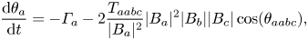 $$\begin{gather}\frac{{\rm d} \theta_a}{{\rm d} t} ={-}\varGamma_a - 2 \frac{T_{aabc}}{|B_a|^2}|B_a|^2|B_b||B_c|\cos(\theta_{aabc}), \end{gather}$$
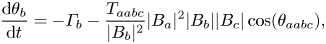 $$\begin{gather}\frac{{\rm d} \theta_b}{{\rm d} t} ={-}\varGamma_b - \frac{T_{aabc}}{|B_b|^2}|B_a|^2|B_b||B_c|\cos(\theta_{aabc}), \end{gather}$$
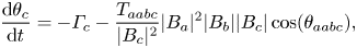 $$\begin{gather}\frac{{\rm d} \theta_c}{{\rm d} t} ={-}\varGamma_c - \frac{T_{aabc}}{|B_c|^2}|B_a|^2|B_b||B_c|\cos(\theta_{aabc}), \end{gather}$$
where  $\theta _{aabc} = \varDelta _{aabc}t - 2\theta _a + \theta _b + \theta _c$ is called the dynamic phase. Note the additional factor of two appearing in the equations for $|B_a|$ and $\theta _a$ because the resonance condition $2\boldsymbol {k}_a = \boldsymbol {k}_b + \boldsymbol {k}_c$ can be satisfied for either the tuple $(\boldsymbol {k}_a,\boldsymbol {k}_a,\boldsymbol {k}_b,\boldsymbol {k}_c)$ or $(\boldsymbol {k}_a,\boldsymbol {k}_a,\boldsymbol {k}_c,\boldsymbol {k}_b)$.
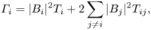 \begin{equation} \varGamma_i = |B_i|^2T_i + 2 \sum_{j\neq i} |B_j|^2 T_{ij}, \end{equation}
where we use an abbreviated notation for the symmetric kernels:  $T_i = T_{iiii}, T_{ij}=T_{ijij}=T_{jiji}$.
The next significant simplification relies on the observation that although there are ostensibly three distinct phases in the equations governing the degenerate quartet (2.4a)–( 2.4f), they occur only in the single combination  $2\theta _a - \theta _b - \theta _c$, which makes it possible to drop subscripts and write $\theta$ and $\varDelta$ in place of $\theta _{aabc}$ and $\varDelta _{aabc}$ without risk of confusion. We can further exploit this fact to combine (2.4d)–( 2.4f) into a single equation for the dynamic phase:
 \begin{equation} \frac{{\rm d} \theta}{{\rm d} t} = \varDelta + 2 \varGamma_a - \varGamma_b - \varGamma_c + T_{aabc} \left( 4 |B_b||B_c| - \frac{|B_c||B_a|^2}{|B_b|} - \frac{|B_b||B_a|^2}{|B_c|}\right) \cos(\theta). \end{equation}
Equations (2.4a)–(2.4c) and (2.6) now form an autonomous system of ordinary differential equations. It is known that this system of equations admits periodic solutions which are given in terms of Jacobi elliptic functions, see Shemer & Stiassnie (Reference Shemer and Stiassnie1985). We shall see that generic solutions are indeed periodic, though we shall focus our attention principally on special, non-periodic solutions. Moreover, we can easily recover the individual phases of the Fourier modes and employ these to reconstruct the leading-order free surface.
The system of (2.4a)–(2.4c) and (2.6) admits the following conserved quantities:
 \begin{equation} |B_a|^2 + |B_b|^2 + |B_c|^2 = A, \end{equation}
the total wave action, and
 \begin{equation} \frac{|B_b|^2}{A} - \frac{|B_c|^2}{A} = \alpha, \end{equation}
the wave-action difference in the two sidebands. These conserved quantities allow us to further reduce the number of parameters by introducing a normalised wave-action variable  $\eta = |B_a|^2/A$, which by (2.7), must take values between $0$ and $1$. The amplitudes may then be rewritten in terms of $\eta$ and $\alpha$ as $|B_a|^2 = A\eta$, $|B_b|^2 = A(1 - \eta + \alpha )/2$ and $|B_c|^2 = A(1 - \eta - \alpha )/2$.
In terms of the two variables  $\eta$ and $\theta$, we find that the system can be described by the Hamiltonian:
 \begin{equation} H(\theta,\eta) ={-}AT_{aabc}2\eta\sqrt{(1 - \eta)^2 - \alpha^2}\cos(\theta) - (\varDelta + A\varOmega_0)\eta - \frac{A\varOmega_1}{2}\eta^2, \end{equation}
with
 $$\begin{gather} \frac{\partial H}{\partial \theta} = \frac{{\rm d} \eta}{{\rm d} t} = 2AT_{aabc}\eta\sqrt{(1 - \eta)^2 - \alpha^2}\sin(\theta), \end{gather}$$
 $$\begin{gather}-\frac{\partial H}{\partial\eta} = \frac{{\rm d} \theta}{{\rm d} t} = \varDelta_{aabc} + A\varOmega_0 + A\varOmega_1\eta + 2AT_{aabc}\frac{1 + 2\eta^2 - 3\eta - \alpha^2}{\sqrt{(1 - \eta)^2 - \alpha^2}}\cos(\theta). \end{gather}$$
The two new coefficients are
 $$\begin{gather} \varOmega_0 = 2 [ T_{ab}(1+\alpha) + T_{ac}(1-\alpha) ] - \tfrac{1}{2}[ T_b (1+\alpha) + T_c (1-\alpha) ] - 2T_{bc}, \end{gather}$$
 $$\begin{gather}\varOmega_1 = 2 ( T_a + T_{bc} ) - 4 ( T_{ab} + T_{ac} ) + \tfrac{1}{2} ( T_b + T_c ). \end{gather}$$
Such a Hamiltonian approach to the three-wave discretisation of the nonlinear Schrödinger equation was first explored by Cappellini & Trillo (Reference Cappellini and Trillo1991), Trillo & Wabnitz (Reference Trillo and Wabnitz1991) in the context of optics, and our Hamiltonian (2.9) can be shown to reduce in the narrowband limit to one analogous to that presented therein.
A final simplification of the system can be achieved by imposing an equidistribution of wave action among the sidebands, i.e.  $\alpha = 0$. Under this assumption, (2.10) and (2.11), as well as the Hamiltonian (2.9), become
 $$\begin{gather} \frac{{\rm d} \eta}{{\rm d} t} = 2AT_{aabc}\eta(1 - \eta)\sin(\theta), \end{gather}$$
 $$\begin{gather} \frac{{\rm d} \theta}{{\rm d} t} = \varDelta + A\varOmega_0 + A\varOmega_1\eta + 2AT_{aabc}(1 - 2\eta)\cos(\theta), \end{gather}$$
 $$\begin{gather}H(\theta,\eta) ={-}2AT_{aabc}\eta(1 - \eta)\cos(\theta) - (\varDelta + A\varOmega_0)\eta -\frac{A\varOmega_1}{2}\eta^2. \end{gather}$$
 In subsequent computations, we shall normalise all wavenumbers by the carrier wavenumber  $k_a$, and all frequencies by the carrier frequency $\omega _a$, which is equivalent to setting the gravitational acceleration $g = 1$. For the unidirectional cases considered, we shall also explicitly specify our degenerate quartets in terms of mode separation $p$ as follows: $\boldsymbol {k}_a = [1,0]$, $\boldsymbol {k}_b = [1 - p,0]$ and $\boldsymbol {k}_c = [1 + p,0]$, where $0< p<1$. We henceforth drop the bold-script and write $k_i$ for the wavenumbers, to emphasise that these are scalars. Indeed, for unidirectional waves in deep water, it is possible to significantly simplify the kernels, as shown by Dyachenko, Kachulin & Zakharov (Reference Dyachenko, Kachulin and Zakharov2017), Kachulin, Dyachenko & Gelash (Reference Kachulin, Dyachenko and Gelash2019) and detailed in Appendix A.
The wave action  $A$ of the three-mode system remains a free parameter and the conservation law (2.7) makes it clear that $A$ may be ‘distributed’ among the three modes in various configurations. The relationship between the complex amplitudes $B_i$ of the Zakharov formulation and the amplitude of the free surface displacement (e.g. (14.5.5) of Mei et al. Reference Mei, Stiassnie and Yue2018, § 14.5) makes it possible to interpret $A$ in terms of the carrier steepness, which is sometimes convenient. If only the carrier wave is present,
 \begin{equation} A = |B_a|^2 = \frac{2 g a^2 {\rm \pi}^2}{\omega_a} = \frac{2 {\rm \pi}^2 g^{1/2} \epsilon^2}{k_a^{5/2}}, \end{equation}
where  $a$ is the surface-wave amplitude and $\epsilon =a k_a$ is the wave slope.
Aside from the wave action  $A$, the system (2.14) and (2.15) contains a further free parameter: the separation between the Fourier modes $p$. Together, these can be used to determine the values of all coefficients in the equation.
3. Hamiltonian dynamics in the phase plane
The Hamiltonian dynamical system (2.14) and (2.15) describes fully the nonlinear dynamics of three interacting deep-water waves. We can gain both qualitative and quantitative understanding of this system via phase-plane analysis, where the phase space is the surface of the truncated cylinder  $\{(\theta,\eta ) \mid -{\rm \pi} \leq \theta \leq {\rm \pi}, 0\leq \eta \leq 1 \}$.
3.1. Fixed points
The first step in unravelling the dynamics is to consider fixed points of our system. The trajectories, corresponding to solutions of the degenerate quartet with particular initial conditions, occupy the level curves of the Hamiltonian (2.16). We find that fixed points of (2.14) and (2.15) occur in four classes:  $\eta = 0$ or 1 and $\theta = 0$ or $\pm {\rm \pi}$. The upper and lower boundaries $\eta =1$ and $\eta =0$ correspond to a single wave train and a bichromatic wave train, respectively (recall $\eta =|B_a|^2/A$). These two well-known solutions of the Zakharov equation exhibit no energy exchange (see Leblanc Reference Leblanc2009 or Mei et al. Reference Mei, Stiassnie and Yue2018, §§ 14.5 & 14.6), since ${\rm d} \eta / {\rm d} t = 0$ thereon. Indeed, the effect of nonlinear interaction in such cases is solely to induce a frequency correction, called Stokes’ correction after Stokes (Reference Stokes1847), and found for bichromatic waves by Longuet-Higgins & Phillips (Reference Longuet-Higgins and Phillips1962); for a discussion in the context of the Zakharov equation, see Stuhlmeier & Stiassnie (Reference Stuhlmeier and Stiassnie2019).
Centre points at  $\theta =0$ and $\theta =\pm {\rm \pi}$ correspond to steady-state near-resonant degenerate quartets of waves. Such solutions have been recently found using the homotopy analysis method (HAM) by Xu et al. (Reference Xu, Lin, Liao and Stiassnie2012), Liao et al. (Reference Liao, Xu and Stiassnie2016), Yang, Yang & Liu (Reference Yang, Yang and Liu2022) and others, for both resonant and near-resonant cases. The dynamics around such points is simple and can be described as time-dependent periodic exchanges of wave energy around the time-independent configuration, as noted by Xu et al. (Reference Xu, Lin, Liao and Stiassnie2012). Exact analytical formulae for such periodic solution can also be obtained in terms of Jacobi elliptic functions, as done by Shemer & Stiassnie (Reference Shemer and Stiassnie1985).
To avoid overly bulky expressions, in what follows, we introduce the following notation:
 \begin{equation} \varDelta' = \frac{\varDelta}{AT_{aabc}}, \quad \varOmega_0' = \frac{\varOmega_0}{T_{aabc}} \quad \text{and}\quad \varOmega_1' = \frac{\varOmega_1}{T_{aabc}}. \end{equation}
In these variables, we obtain fixed points at  $\eta =1$ of the form $(\theta,\eta )=(\theta _{\pm 1},1)$ whenever $\theta _{ 1}$ satisfies
 \begin{equation} \cos(\theta_1) = \frac{\varDelta' + \varOmega_0' + \varOmega_1'}{2}. \end{equation}
Such fixed points exist when the right-hand side is between  $-$1 and 1, and $\theta _{-1} = -\theta _1$. These fixed points lie on the contour $H=-\varDelta - A\varOmega _0 - {A\varOmega _1}/{2}$. Similarly, we obtain fixed points at $\eta =0$ of the form $(\theta,\eta )=(\theta _{\pm 0},0)$ whenever $\theta _{ 0}$ satisfies
 \begin{equation} \cos(\theta_0) ={-}\frac{\varDelta' + \varOmega_0'}{2}, \end{equation}
again provided the right-hand side is between  $-$1 and 1 and $\theta _{-0} = -\theta _0$. These fixed points lie on the contour $H=0$. Another class of fixed points is obtained for $\theta =0$ or $\pm {\rm \pi}$. In the former case, $(\theta,\eta )=(0,\eta _0)$ is a fixed point whenever
 \begin{equation} \eta_0 = \frac{2 + \varDelta' + \varOmega_0'}{4 - \varOmega_1'}, \end{equation}
and  $0\leq \eta _0 \leq 1$. Note that $\eta _0 = 1$ if and only if $\theta _{\pm 1} = 0$, in which case, this fixed point coincides with (3.2). For $\theta =\pm {\rm \pi}$, we find fixed points $(\pm {\rm \pi},\eta _{\rm \pi} )$ provided
 \begin{equation} \eta_{\rm \pi} = \frac{2 - (\varDelta' + \varOmega_0')}{4 + \varOmega_1'}, \end{equation}
and  $0\leq \eta _{\rm \pi} \leq 1$. Similarly, $\eta _{\rm \pi} = 0$ if and only if $\theta _{\pm 0} = \pm {\rm \pi}$, such that this fixed point coincides with (3.3).
3.2. Phase portraits and bifurcation
The dynamical system (2.14) and (2.15) contains two parameters – wave action  $A$ and mode-separation $p$ – which together govern the existence of the fixed-points given in (3.2)–(3.5), and the attendant dynamics. The natural choice is to fix $A$ – akin to specifying the total energy of waves – and to use mode separation as a bifurcation parameter.
In figure 1, we depict a series of characteristic phase portraits, where mode separation  $p$ increases from $p=0$ in panel (a) to $p=0.3$ in panel (h). In this figure, we have selected $A$ equivalent to a carrier wave with steepness $\epsilon =0.1$, so that $A=2 {\rm \pi}^2/100$ (see (2.17) and recall $g=k_a=1$). The figure thus represents both physically realistic, as well as characteristic behaviour, in a sense to be specified in detail below.

Figure 1. Phase portraits for  $A=2 {\rm \pi}^2/100$ and various values of mode separation $p$ between 0 and 0.3, plotted on the cylinder $\{(\eta,\theta )\mid \eta \in [0,1], \theta \in [-{\rm \pi},{\rm \pi} ]\}$. Coloured curves represent contours of the Hamiltonian (2.16). Dashed lines show separatrices, while dots denote fixed-points of the system. (a) $p=0$, (b) $p=0.06$, (c) $p=0.0908771$, (d) $p=0.1$, (e) $p=0.120902$, ( f) $p=0.2$, (g) $p=0.246206$ and (h) $p=0.3$.
Deferring the details for the moment, we can give an overview of the dynamics of our degenerate quartet as obtained by phase-plane analysis, and shown in figure 1. In the limit of vanishing mode separation, figure 1(a), we find four fixed points: a centre at  $\theta =0$, a pair of saddle points on $\eta =0$, located at $\theta =\pm 2{\rm \pi} /3$, and a semi-stable fixed point at $\theta =\pm {\rm \pi}, \eta =1$. The first bifurcation occurs at $p=0$, and as $p$ increases, the semi-stable point at $(\theta,\eta )=(\pm {\rm \pi},1)$ splits into three fixed points: a centre at $\theta =\pm {\rm \pi}$ and two saddles at $\eta =1$ (figure 1b). Further increase in the mode separation causes the centre at $\theta =\pm {\rm \pi}$ to descend until the saddle connections between the two fixed points at $\eta =0$ and $\eta =1$ merge (figure 1c). This critical value of mode separation exhibits the maximal energy exchange among the interacting modes.
Further increasing  $p$ leads the centre at $\theta =\pm {\rm \pi}$ to descend towards $\eta =0$ (figure 1d) where it subsequently vanishes together with the saddle points along $\eta =0$ (figure 1e). As the modes are separated further, the remaining three fixed points draw closer together in phase space (figure 1 f) before coalescing (figure 1g) and disappearing entirely (figure 1h) – this last bifurcation leads to complete stabilisation of the system.
Separatrices (shown as dashed lines in figure 1) partition the phase plane. For example, in figure 1(a), we notice that interior solutions with initial values  $\theta (0)<-2{\rm \pi} /3$ or $\theta (0)>2{\rm \pi} /3$ are periodic and wind around the exterior of the separatrix connecting the pair of fixed points at $\eta =0$. Such solutions take on all values of the phase from $-{\rm \pi}$ to ${\rm \pi}$. Other periodic solutions are confined to the interior of the separatrix, and wind around the centre at $\theta =0$.
4. Nonlinear stability
While the phase-plane analysis presented above is remarkably simple, it contains a wealth of information about the fully nonlinear dynamics of interacting degenerate quartets of deep water waves. We focus first on a discussion of nonlinear instability results.
4.1. Nonlinear instability of a uniform wave train
Many classical studies of the stability of a uniform wave train begin by establishing that such a monochromatic wave is a solution of the relevant governing equation. This solution is then used as a starting point for linearisation and an instability criterion derived from the eigenvalues of the linear system, as done by Crawford et al. (Reference Crawford, Lake, Saffman and Yuen1981). In our framework, uniform wave trains are described by  $\eta =1$, for arbitrary values of $\theta$. The initial small disturbance used classically to investigate the Benjamin–Feir instability consists in imposing small sidebands, i.e. a shift to a contour $\eta <1$. In figure 1(a–f), we readily observe that such a shift leads to growth of the sidebands, as $\eta$ decreases along the contours, followed generically by periodic energy exchange. Maximal energy exchange occurs when $\eta$ is changing fastest, and coincides with the smallest changes in the dynamic phase $\theta$. Such phase coherence has also been observed in simulations, e.g. by Houtani, Sawada & Waseda (Reference Houtani, Sawada and Waseda2022) and Liu, Waseda & Zhang (Reference Liu, Waseda and Zhang2021).
In fact, we can show that the classical linear stability criterion is equivalent to the existence of fixed points at  $\eta = 1$ in the nonlinear system. The condition (3.2) for such fixed points to exist is
 \begin{equation} -1 \leq \frac{\varDelta' + \varOmega_0' + \varOmega_1'}{2}\leq 1. \end{equation}
Squaring these inequalities, substituting  $\varOmega _0$ and $\varOmega _1$ from (2.12) and (2.13), and using (2.17) yields, after simplification, the discriminant criterion
 \begin{equation} \left(\frac{\varDelta}{2} + (T_a - T_{ab} - T_{ac})|B_a|^2\right)^2 - |B_a|^4T_{aabc}^2\leq 0, \end{equation}
see (Mei et al. Reference Mei, Stiassnie and Yue2018, (14.9.16)). It is rather surprising that this eigenvalue condition, which arises from an approach based on small amplitude perturbations (and which is oblivious to the existence of fixed-points of the original nonlinear problem), can be recovered exactly with our approach.
4.1.1. Stability boundaries and restabilisation
The existence of fixed points at  $\eta =1$, and thus the instability of uniform wave trains to some perturbation, is the generic situation for degenerate quartets. We can appreciate this by considering (3.2), from which we establish that fixed points exist at $\eta =1$ for some mode separation, provided $A \in [ 0 , {2 {\rm \pi}(2-\sqrt {2}) \sqrt {g}}{k_a^{-5/2}} ].$ Employing (2.17), this can be expressed in terms of carrier wave slope $\epsilon$ and implies the existence of fixed points (and thus instability) for
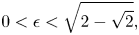 \begin{equation} 0 < \epsilon < \sqrt{2-\sqrt{2}}, \end{equation}
far beyond the wave breaking threshold.
In the limit of small mode separation, when the wavelengths of the sidebands are comparable to the carrier, we see that the instability domain remains bounded (see figure 2), with fixed points for  $A \in [0,{\sqrt {g k_a}{\rm \pi} ^2}/{3 k_a}]$. This yields the threshold
 \begin{equation} 0 < \epsilon < \frac{1}{\sqrt{6}}, \end{equation}
which has previously been obtained numerically (see e.g. Yuen & Lake Reference Yuen and Lake1982, § VI.B.1). The simple, explicit formulae (4.3)–(4.4) presented here are the results of compact forms of the one-dimensional interaction kernels which allow for considerable algebraic simplification (see Appendix A and Kachulin et al. Reference Kachulin, Dyachenko and Gelash2019).
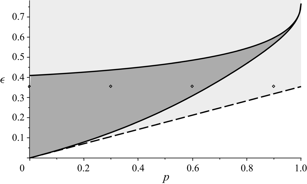
Figure 2. Existence of  $\eta =1$ fixed points in $(\epsilon,p)$-parameter space according to (3.2). The dark shaded region denotes the nonlinear instability domain for the degenerate quartet. The dashed line denotes the lower boundary of the NLS instability threshold $\epsilon = p/\sqrt {8}$, which is shown in the light shaded region. For markers, refer to Appendix B.
In fact, this restabilisation for nearby sidebands (or long-wavelength disturbances) is a characteristic of the broadbanded Zakharov equation. Indeed, imposing a limit of narrow spectral bandwidth (in which the Zakharov equation reduces to the NLS) implies
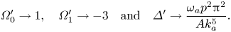 \begin{equation} \varOmega'_0 \rightarrow 1, \quad \varOmega'_1 \rightarrow -3 \quad \text{and}\quad \varDelta' \rightarrow \frac{\omega_a p^2 {\rm \pi}^2}{A k_a^5}. \end{equation}
This can be used to reformulate the fixed-point criterion and recover the well-known instability threshold for NLS (Mei et al. Reference Mei, Stiassnie and Yue2018, (14.9.21)):
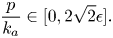 \begin{equation} \frac{p}{k_a} \in [ 0,2\sqrt{2} \epsilon]. \end{equation}
This is plotted in the  $(p,\epsilon )$-domain as the lightly shaded region above the dashed line $\epsilon =p/\sqrt {8}$ in figure 2. For small mode-separation distance $p$, the NLS instability criterion agrees well with the more general formulation of the Zakharov equation, as shown previously by Yuen & Lake (Reference Yuen and Lake1982). However, the linear stability analysis of the NLS yields instability to perturbations with arbitrary separation provided the steepness $\epsilon$ is sufficiently large (see Appendix B for a comparison of the phase portraits).
For the truncated Zakharov equation, as mode-separation increases, larger values of carrier steepness  $\epsilon$ are required to generate instability, up to the limit $p=1$ when the instability domain contracts to the point $\epsilon = \sqrt {2-\sqrt {2}}$. Conversely, for a given carrier steepness and increasing mode separation, the system will eventually exit the instability domain – this bifurcation is captured in figure 1(g), where fixed points at $\eta =1$ coalesce and disappear.
4.2. Nonlinear stability of a bichromatic wave train
Instabilities of bichromatic wave trains, while less well-known than those for uniform wave trains, have also been studied, for example, by Leblanc (Reference Leblanc2009), Badulin et al. (Reference Badulin, Shrira, Kharif and Ioualalen1995) or Ioualalen & Kharif (Reference Ioualalen and Kharif1994). While our setting is somewhat different – in particular, we have only three unidirectional modes, in contrast to the four modes used by Leblanc Reference Leblanc2009, § 4 to discuss class Ib instabilities – we can nevertheless obtain the nonlinear evolution of such instabilities by our phase-plane analysis, recalling that a bichromatic wave train occupies the line  $\eta =0$. In the present case, where the Fourier amplitudes of the sidebands $k_b$ and $k_c$ are taken to be identical, we naturally have a bichromatic wave train with waves of different steepness. Mode $k_b=(1-p,0)$ corresponds to a longer wave than mode $k_c=(1+p,0)$, and their slopes are related as
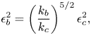 \begin{equation} \epsilon_b^2 = \left( \frac{k_b}{k_c} \right)^{5/2} \epsilon_c^2, \end{equation}
see Mei et al. (Reference Mei, Stiassnie and Yue2018, § 14.6). Without loss of generality, we depict the instability domain in terms of  $\epsilon _b$ in figure 3.
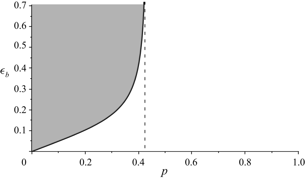
Figure 3. Existence of  $\eta =0$ fixed points in $(\epsilon _b,p)$-parameter space, according to (3.3). The shaded region denotes the instability domain for a bichromatic wave train with equipartitioned mode amplitudes.
The existence of fixed points – and consequent instability – of the bichromatic wave train is again seen to be generic. For any wave train, there exists a value of mode separation  $p$ such that the solution is unstable within the framework of the degenerate quartet. This wave train stabilises for sufficiently large mode separation, as seen in the bifurcation in figure 1(e), when fixed points at $\eta =0$ disappear. Moreover, we find a critical threshold for mode separation $p\approx 0.42$ beyond which bichromatic wave trains are stable.
5. Heteroclinic solutions
The existence of special solutions to the nonlinear Schrödinger equation (NLS) has attracted considerable attention in recent years, a discussion of which may be found in the work by Dysthe & Trulsen (Reference Dysthe and Trulsen1999) or, with an emphasis on hydrodynamics and experimental verification, by Chabchoub et al. (Reference Chabchoub, Kibler, Dudley and Akhmediev2014) and the references therein. We will see that several remarkable solutions – corresponding to heteroclinic orbits in the phase plane – exist for the three wave system. These include a discrete breather, i.e. a breather with finite spectral content, analogous to that found by Akhmediev, Eleonskiĭ & Kulagin (Reference Akhmediev, Eleonskiĭ and Kulagin1987), Ablowitz & Herbst (Reference Ablowitz and Herbst1990), which approaches a plane wave as  $t\rightarrow \pm \infty$. The form of the free surface and its envelope are of particular interest for such solutions; these can be recovered from the solution of the Zakharov equation (2.1) by defining the following complex amplitude function:
 \begin{equation} A(x,t) = \frac{1}{\rm \pi}\left(\sqrt{\frac{\omega_a}{2g}}B_a\, {\rm e}^{{\rm i}(k_ax - \omega_a t)} + \sqrt{\frac{\omega_b}{2g}}B_b\, {\rm e}^{{\rm i}(k_bx - \omega_b t)} + \sqrt{\frac{\omega_c}{2g}}B_c\, {\rm e}^{{\rm i}(k_cx - \omega_c t)}\right). \end{equation}
The free surface elevation is then obtained as
 \begin{equation} \zeta(x,t) = \Re[A(x,t)], \end{equation}
and the envelope is  $|A(x,t)|$.
5.1. Discrete breather solutions
The existence of special heteroclinic solutions, with properties similar to the well-known breather solutions of the nonlinear Schrödinger equation, clearly depends on the fixed points of our problem. Our approach is akin to that of Cappellini & Trillo (Reference Cappellini and Trillo1991), who first investigated a three-mode truncation of the nonlinear Schrödinger equation.
5.1.1. The discrete (1-1) Akhmediev breather
For values of  $p$ and $A$ satisfying (3.2) (see § 4.1 and figure 2), the two saddle points $(\theta,\eta )=(\pm \theta _1,1)$ are connected by a heteroclinic orbit. Along this orbit, $\eta <1$ and a trajectory approaches $(\pm \theta _1,1)$ as $t\to \pm \infty$.
In fact, we can compute these solutions explicitly, by considering the following set of equations:
 $$\begin{gather} 2\eta\cos(\theta) = \varDelta' + \varOmega_0' + \frac{\varOmega_1'}{2}(1 + \eta), \end{gather}$$
 $$\begin{gather}\frac{{\rm d} \eta}{{\rm d} \theta} = \frac{\eta\sin(\theta)}{\cos(\theta) - \dfrac{\varOmega_1'}{4}}, \end{gather}$$
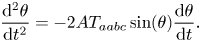 $$\begin{gather}\frac{{\rm d}^2\theta}{{\rm d} t^2} ={-}2AT_{aabc}\sin(\theta)\frac{{\rm d} \theta}{{\rm d} t}. \end{gather}$$
Equation (5.3a) follows from equating the Hamiltonian (2.16) to its value at  $\eta = 1$. Equation (5.3b) is obtained from the implicit function theorem by regarding $\eta$ as a function of $\theta$ instead of $t$. Equation (5.3c) is obtained by taking the time derivative of (2.15). Equation (5.3a) is further used to simplify the form of (5.3b) and (5.3c).
Equation (5.3b) is separable and can be integrated directly to give
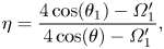 \begin{equation} \eta = \frac{4\cos(\theta_1) - \varOmega_1'}{4\cos(\theta) - \varOmega_1'}, \end{equation}
where the integration constant is chosen so that the limits as  $\theta$ tends to $\pm \theta _1$ are 1.
Equation (5.3c) can also be integrated to obtain
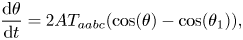 \begin{equation} \frac{{\rm d} \theta}{{\rm d} t} = 2AT_{aabc}(\cos(\theta) - \cos(\theta_1)), \end{equation}
where the integration constant is chosen so that the limits as  $\theta$ tends to $\pm \theta _1$ are 0. Integrating again yields an expression for the dynamic phase:
 \begin{equation} \tan(\theta/2) = \tan(\theta_1/2)\tanh(AT_{aabc}\sin(\theta_1)t), \end{equation}
where the integration constant was chosen so that  $\theta (0) = 0$. Together, (5.6) and (5.4) describe the heteroclinic orbits shown in figure 1(d–f). (Note that the heteroclinic orbits around $\theta =\pm {\rm \pi}$ in figure 1(b) can be treated similarly.)
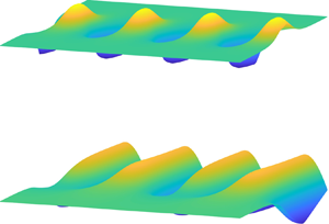
The discrete (1-1) Akhmediev breather describes an orbit in phase space which connects one plane-wave solution with another. During the initial evolution, energy is transferred to the sidebands ( $\eta$ decreases) while the dynamic phase undergoes little change. Subsequent to this focusing, the energy-transfer process reverses, resulting in a phase-shifted plane wave. This situation is depicted in dimensionless coordinates in figure 4(a,b). Figure 4(a) shows the envelope, which is periodic in space and ‘breathes’ once at time ${t}=0$, akin to the Akhmediev breather solution of the NLS. Figure 4(b) shows the free surface, which begins as a monochromatic plane wave, grows into a strongly modulated wave-train at ${t}=0$ and reverts to a plane wave with an evident phase shift.
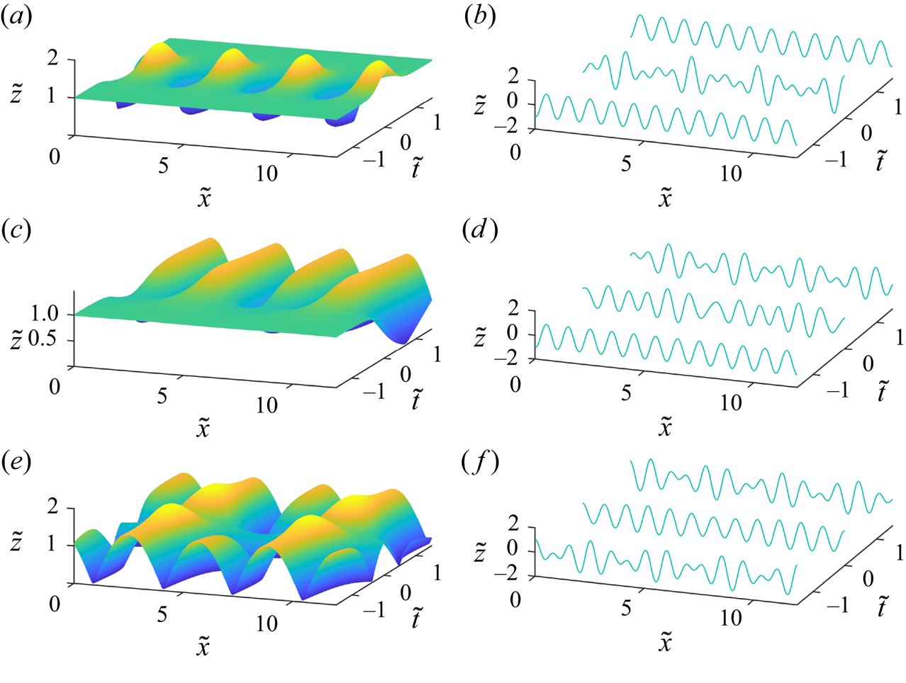
Figure 4. Time evolution of (a,c,e) the envelopes and (b,d,f) the free surface along different heteroclinic solutions. In all cases, the steepness of the wave  $k_a$ is set to $\epsilon _a = 0.2$. (a,b) Discrete Akhmediev breather for $p = 0.3012$; (c,d) (1-0) breather for the critical $p = 0.1670$; (e, f) (0-0) breather for $p = 0.1570$. Here, $\tilde {x} = x k_a/2{\rm \pi}$, $\tilde {t} = t\omega _a/2{\rm \pi}$ and $\tilde {z} = z/\epsilon _a.$
The discrete Akhmediev breather which occurs in the study of a single degenerate quartet is, in fact, the skeleton of the famed Akhmediev breather solution of the nonlinear Schrödinger equation; the latter likewise arises from the instability of a carrier wave and two equidistant sidebands, which subsequently induces a cascading instability as described by Chin, Ashour & Belić (Reference Chin, Ashour and Belić2015). This makes a direct comparison possible, at least for the Fourier modes  $A_0$ and $A_{1}$ of the Akhmediev breather ( $A_{-1}$ evolves analogously to $A_1$).
From Chin et al. (Reference Chin, Ashour and Belić2015), we obtain the following exact equations for the Fourier modes of the Akhmediev breather:
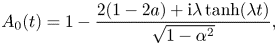 $$\begin{gather} A_0(t) = 1 - \frac{2(1 - 2a) + {\rm i}\lambda\tanh(\lambda t)}{\sqrt{1 - \alpha^2}}, \end{gather}$$
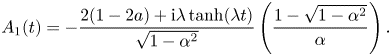 $$\begin{gather}A_1(t) ={-}\frac{2(1 - 2a) + {\rm i}\lambda\tanh(\lambda t)}{\sqrt{1 - \alpha^2}}\left(\frac{1 - \sqrt{1 - \alpha^2}}{\alpha}\right). \end{gather}$$
The parameters  $a$,
$a$,  $\alpha$ and $\lambda$ can be related to our parameters $p$,
$p$,  $\epsilon _a$ as follows:
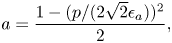 $$\begin{gather} a = \frac{1 - (p/(2\sqrt{2}\epsilon_a))^2}{2}, \end{gather}$$
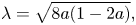 $$\begin{gather}\lambda = \sqrt{8a(1 - 2a)}, \end{gather}$$
 $$\begin{gather}\alpha = \frac{\sqrt{2a}}{\cosh(\lambda t)}. \end{gather}$$
This ensures that we are comparing discrete and continuous Akhmediev breathers with the same spatial periodicity.
Figure 5 shows the time evolution of the carrier (blue curves) and one of the sidebands (red curves; recall that these evolve symmetrically) for the Akhmediev breather (dashed curves) and our discrete breather (solid curves). We take  $\epsilon _a = 0.2$ with $p =$ 0.1, 0.3 and 0.4 in each panel from top to bottom, respectively, and use the dimensionless time $\tilde {t} = AT_{aabc}t$.
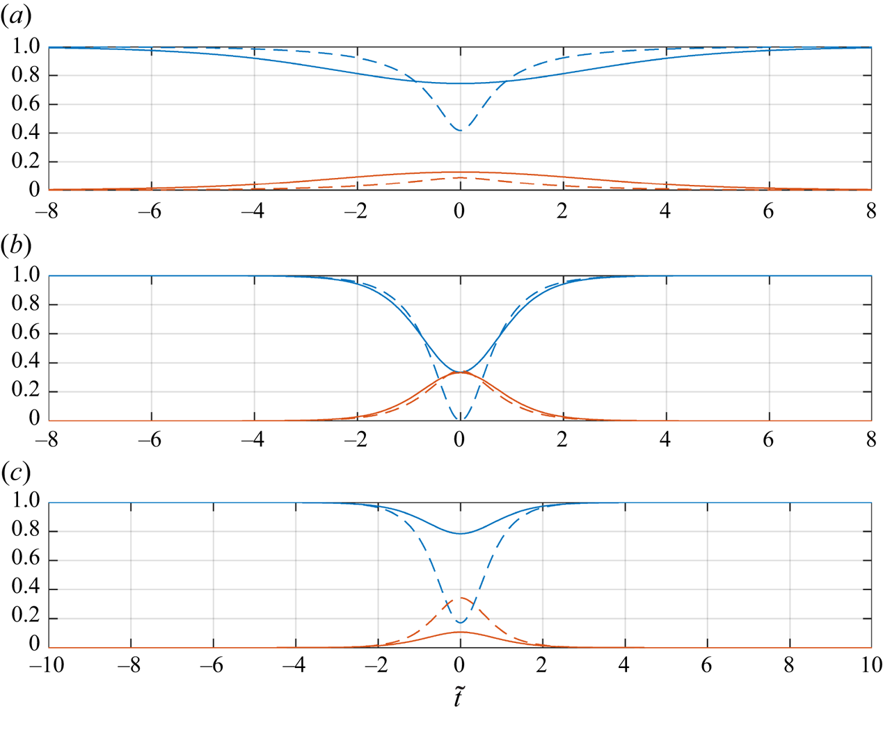
Figure 5. Comparison of the (1-1) discrete breather (solid lines) with the Akhmediev breather (dashed lines). Blue lines, time evolution of the carrier ( $|B_a|^2$ and $|A_0|^2$, respectively). Red lines, time evolution of the sideband ( $|B_b|^2$ and $|A_1|^2$, respectively). In all cases, $\epsilon _a = 0.2$. (a) $p = 0.1$. (b) $p = 0.3$. (c) $p = 0.4$.
There is qualitative resemblance and a degree of quantitative agreement in the evolution of the continuous breather and our three-mode model, particularly for intermediate mode separation and wave slope. However, as elucidated by Chin et al. (Reference Chin, Ashour and Belić2015), the formation of the Akhmediev breather takes the form of an energy cascade wherein the energy of the carrier mode is distributed among all the infinite Fourier modes at  $t = 0$. Since our model is truncated to three Fourier modes (the carrier wave and its sidebands only), this energy cascade is also truncated, leading to a surplus of energy remaining in the carrier wave simply because there are no more modes in the system. This is seen in figure 5 at $t=0$, where the solid blue lines (modes $|B_a|$) sit above the dashed blue lines (modes $|A_0|$).
Figure 5(c) also illustrates the main difference between the Zakharov equation and the NLS for unidirectional waves, namely the difference in stability of a monochromatic wave train. The case  $p=0.4$ (figure 5c) is very close to the border of our stability region plotted in figure 2. Hence, the small energy exchange observed at $\tilde {t} = 0$. Once $p$ is outside the instability region, there is no energy exchange (the phase portraits are akin to figure 1h) and no discrete breather solutions exist. The larger instability domain of the NLS, in contrast, continues to allow breather solutions, as reflected in the considerable energy exchange seen in figure 5(c) (dashed lines).
5.1.2. (1-0) breather and (0-1) breathers
A special type of heteroclinic solution appears when the Hamiltonian at  $\eta = 1$ vanishes, i.e. when $p$ and $A$ are such that $\varDelta ' + \varOmega _0' + \varOmega _1'/2 = 0$. There are two such heteroclinic solutions, one linking fixed points $(\theta _0,0)$ and $(\theta _1,1)$, and the other linking $(-\theta _1,1)$ with $(-\theta _0,0)$ (see figure 1c). These appear also in the context of optical fibres when the governing equation is the NLS, and are referred to as ‘pump-depletion’ solutions by Cappellini & Trillo (Reference Cappellini and Trillo1991).
In this case, (2.14) simplifies to
 \begin{equation} \frac{{\rm d} \eta}{{\rm d} t} ={\pm} A T_{aabc} \eta(1 - \eta)\sqrt{4 - \frac{{\varOmega_1'}^2}{4}}, \end{equation}
where the sign depends on which fixed point we are considering. Integrating this equation yields
 \begin{equation} \eta = \frac{{\rm e}^{{\pm} A T_{aabc}\sqrt{4 - \dfrac{{\varOmega_1'}^2}{4}} t + C}}{{\rm e}^{{\pm} A T_{aabc}\sqrt{4 - \dfrac{{\varOmega_1'}^2}{4}} t + C} + 1}, \end{equation}
where  $C$ is an integration constant depending on the initial conditions. For instance, $C = 0$ for the initial condition $\eta (0) = \frac {1}{2}$. Assuming that a positive sign is chosen, the solution tends to $1$ as $t\to \infty$ and it tends to $0$ as $t\to -\infty$. The limits are reversed if the negative sign is chosen.
The special case described by these orbits corresponds to a complete energy transfer from a uniform wave train to a bichromatic wave train (or vice versa), which appears hitherto not to have been observed in water waves. The envelope and free surface are depicted in figures 4(c) and 4(d), respectively. These show how spatially periodic modulation appears ‘out of nowhere’ with time  ${t}$, or disappears as time is traversed in the negative sense.
5.1.3. (0-0) breather
For a given (sub-critical) value of mode separation  $p$, and $A$ such that (3.3) is satisfied (see 4.2 and figure 3), two distinct fixed points $(\theta,\eta )=(\pm \theta _0,0)$ are linked by a heteroclinic solution that approaches $(\pm \theta _0,0)$ as $t\to \mp \infty$, and along which $\eta > 0$. This solution satisfies the following set of equations:
 $$\begin{gather} 2(\eta - 1)\cos(\theta) = \varDelta' + \varOmega_0' + \eta \frac{\varOmega_1'}{2}, \end{gather}$$
 $$\begin{gather}\frac{{\rm d} \eta}{{\rm d} \theta} = \frac{(1 - \eta)\sin(\theta)}{\dfrac{\varOmega_1'}{4} - \cos(\theta)}, \end{gather}$$
 $$\begin{gather}\frac{{\rm d}^2\theta}{{\rm d} t^2} = 2A T_{aabc}\sin(\theta)\frac{{\rm d} \theta}{{\rm d} t}. \end{gather}$$
As above, (5.14a) has been used to simplify (5.14b) and (5.14c).
Integrating (5.14b) yields
 \begin{equation} \eta = 2\frac{2\cos(\theta) + \varDelta' + \varOmega_0'}{4\cos(\theta) - \varOmega_1'} = \frac{4\cos(\theta) - 4\cos(\theta_0)}{4\cos(\theta) - \varOmega_1'}, \end{equation}
where the integration constant is chosen so that the limits as  $\theta$ tends to $\theta _0$ are 0.
Integrating (5.14c) yields
 \begin{equation} \frac{{\rm d} \theta}{{\rm d} t} ={-}2A T_{aabc} (\cos(\theta) - \cos(\theta_0)), \end{equation}
where the integration constant is chosen so the limits as  $\theta$ tends to $\pm \theta _0$ are 0. Further integration yields
 \begin{equation} \tan(\theta/2) ={-}\tan(\theta_0/2)\tanh (\sin(\theta_0) A T_{aabc} t). \end{equation}
 This solution is the natural counterpart to the discrete Akhmediev breather presented in § 5.1.1; however, rather than tending to a uniform wave train with  $t\rightarrow \pm \infty$, it tends to a bichromatic wave train, again with an attendant phase shift. The envelope and free surface for such a case are shown in figures 4(e) and 4( f), respectively. At ${t}=0$, the modulation is at a minimum, and the free surface elevation is close to a uniform wave train.
5.2. Limiting solutions
It is clear from (2.16) that the horizontal lines  $\eta = 1$ and $\eta = 0$ are level lines of the Hamiltonian. Hence, any solution of (2.14) and (2.15) with suitable initial conditions so that $\eta = 1$ or $\eta = 0$ will remain on these lines.
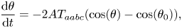
As with the fixed points themselves, there is no energy exchange among the wave modes for these solutions. However, they are not steady (or stationary) solutions in the usual sense, because  $\theta$ still satisfies the following differential equation:
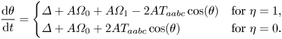 \begin{equation} \frac{{\rm d} \theta}{{\rm d} t} = \begin{cases} \varDelta + A\varOmega_0 +A\varOmega_1 - 2AT_{aabc}\cos(\theta) & \text{for $\eta = 1$,}\\ \varDelta + A\varOmega_0 + 2AT_{aabc}\cos(\theta) & \text{for $\eta = 0$.} \end{cases} \end{equation}
A further differentiation of these equations with respect to  $t$ yields (5.3c) and (5.14c) respectively, which means that (5.6) and (5.17) are solutions for each case. Both limiting configurations of the system exhibit what is sometimes referred to as phase-locking or phase coherence; whereby, regardless of the initial phase, the dynamic phase converges to the fixed value $-\theta _1$ at $\eta = 1$ and $\theta _0$ at $\eta = 0$. It is expected that if initial conditions are taken close to $\eta = 1$, i.e. if some small amount of energy is initially put in the sidebands, then a similar behaviour will be observed in the evolution of the combined phase, as has been recently reported by Houtani et al. (Reference Houtani, Sawada and Waseda2022).
From the mathematical point of view, both limiting configurations  $\eta =1$ and $\eta =0$ of the system can be understood as the limit of the generic periodic solutions, as all the energy goes to either the wave $k_a$, or is equipartitioned among the sidebands $k_b$ and $k_c$, respectively. From a physical point of view, the dynamic phase $\theta$ disappears at both $\eta = 1$ or $\eta = 0$ configurations and one is left with a classical monochromatic Stokes waves or two co-propagating Stokes waves, respectively.
6. Discussion and conclusions
The reformulation of the discrete Zakharov equation for three modes as a two-dimensional Hamiltonian dynamical system provides a new and powerful perspective on a classical problem. In fact, the possibility of reformulating the Zakharov equations for a degenerate quartet in terms of only two auxiliary variables is intimately connected to the existence of an exact solution for this configuration, which can be given in terms of elliptic functions (see Shemer & Stiassnie Reference Shemer and Stiassnie1985). With subsequent normalisations, it is possible to effectively describe the entire dynamics in terms of the total wave action  $A$ and a single bifurcation parameter $p$, the mode separation.
The mode separation governs the appearance of fixed points in the phase plane. Saddle points at  $\eta =1$ and $\eta =0$ correspond to cases where the entire energy is concentrated in one or two Fourier modes, respectively; the centres correspond to a degenerate quartet of nearly resonant waves which undergoes no time evolution. These fixed points are simply another case of the steady-state waves recently discovered by Liao et al. (Reference Liao, Xu and Stiassnie2016), Yang et al. (Reference Yang, Yang and Liu2022). Our phase-plane analysis provides a simple way to obtain these solutions, and highlights for the first time their critical role in organising the overall dynamics.
The existence of fixed-points on the boundaries  $\eta =1$ and $\eta =0$ of our phase-space is intimately connected with the stability of uniform and bichromatic wave trains, respectively. When such fixed points are absent, the trajectories progress along nearly horizontal level lines on the cylindrical phase plane: the dynamic phase changes, but there is little redistribution of energy. Loosely speaking, we may say that the trajectories do not need to avoid the separatrices connecting the fixed points. The stability results we obtain for uniform wave trains demonstrate the robustness of the Benjamin–Feir condition, which we recover from the fully nonlinear system without any small-amplitude assumptions. For bichromatic wave trains, our setting appears to be different from those previously studied, and no comparable linear results appear to be available.
We also obtain numerous special solutions – including discrete breathers – which are identified with heteroclinic orbits in phase space. While the breather solutions of the nonlinear Schrödinger equation involve a continuum of modes, and therefore exhibit quantitatively different features, the two-dimensional phase space allows for an incisive and transparent analysis of these special solutions. It should be noted that, although breathers have sometimes been identified with homoclinic orbits, this terminology obscures the phase shift which is apparent in the heteroclinic connections between the saddle points.
The discrete breather solutions we obtain include an analogue of the Akhmediev breather, which arises from a plane-wave background, as well as limiting cases in which a uniform wave train becomes (as  $t\rightarrow \infty$) a bichromatic wave train, and vice versa. While discrete Akhmediev breathers exist in large ranges of parameter space (and thus for many configurations of total energy and mode separation), the limiting (0,1) and (1,0) breathers are unique for given wave action $A$ or mode separation $p$. In the context of water waves, we also find a seemingly new type of breather-like solution, which arises from, and returns to, a bichromatic background. The maximal energy exchange for this (0,0)-breather is therefore a ‘demodulation’, in which the envelope flattens out.
Breather-solutions of the continuous nonlinear Schrödinger equation have received considerable attention in recent years, both in fluid mechanics and optics (Mussot et al. Reference Mussot, Naveau, Conforti, Kudlinski, Copie, Szriftgiser and Trillo2018; Pierangeli et al. Reference Pierangeli, Flammini, Zhang, Marcucci, Agranat, Grinevich, Santini, Conti and DelRe2018; Vanderhaegen et al. Reference Vanderhaegen, Naveau, Szriftgiser, Kudlinski, Conforti, Mussot, Onorato, Trillo, Chabchoub and Akhmediev2021). While our new discrete breathers have some qualitative similarity with those obtained in the continuous model, there are notable quantitative differences. In particular, in our context, only three modes can be activated, so there is a limit to the cascading instability observed in the formation of the Akhmediev breather solution (Chin et al. Reference Chin, Ashour and Belić2015). This engenders differences in the breather's formation time, as well as in the maximum amplification. In a more general sense, the modulational instability of a single degenerate quartet – as considered in the present paper – captures many of the salient features of the Akhmediev breather, while significantly constraining the phase-space. Indeed, as more modes are considered, the dynamics can become chaotic (Annenkov & Shrira Reference Annenkov and Shrira2001), and the integrable three-mode theory we consider cannot capture the richness of possible behaviours.
Together with theoretical advances, there have been numerous recent experimental breakthroughs in the observation of breather solutions in water wave tanks (Chabchoub, Hoffmann & Akhmediev Reference Chabchoub, Hoffmann and Akhmediev2011; Chabchoub et al. Reference Chabchoub, Hoffmann, Onorato and Akhmediev2012; Kimmoun et al. Reference Kimmoun2016; Gomel et al. Reference Gomel, Chabchoub, Brunetti, Trillo, Kasparian and Armaroli2021). In an experimental context, the waves evolve in space rather than time, and the evolution equations must be changed to reflect this: for unidirectional waves, the temporal Zakharov equation (2.1) can be replaced by an analogous spatial Zakharov equation, derived by Shemer et al. (Reference Shemer, Jiao, Kit and Agnon2001), Shemer, Kit & Jiao (Reference Shemer, Kit and Jiao2002). The extent to which the new breathers agree with flume experiments poses an interesting question for future work.
Acknowledgements
We would like to thank the anonymous referees for numerous comments and suggestions which helped to improve the manuscript.
Funding
This work was supported by the Engineering & Physical Sciences Research Council (grant number EP/V012770/1).
Declaration of interests
The authors report no conflict of interest.
Appendix A. Interaction kernels
The interaction kernels appearing in the Zakharov equation (2.4) are lengthy, and expressions for these can be found in works by Mei et al. (Reference Mei, Stiassnie and Yue2018) and Krasitskii (Reference Krasitskii1994). For the case of unidirectional waves in deep water ( $k_i>0$ for all $i$) treated in the present study, considerable simplifications to the kernels are possible:
 $$\begin{gather} T(k,k,k,k)=\frac{k^3}{4 {\rm \pi}^2}, \end{gather}$$
 $$\begin{gather}T(k_a,k_b,k_a,k_b)=\frac{1}{4 {\rm \pi}^2} k_a k_b \min(k_a,k_b), \end{gather}$$
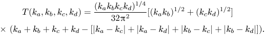 \begin{gather} T(k_a,k_b,k_c,k_d)=\frac{(k_a k_b k_c k_d)^{1/4}}{32 {\rm \pi}^2} [ (k_a k_b)^{1/2} + ( k_c k_d )^{1/2} ]\nonumber\\ \quad \times\ ( k_a + k_b + k_c + k_d - [ |k_a - k_c| + |k_a-k_d| +|k_b-k_c| + |k_b-k_d| ]). \end{gather}
The equation for  $T_{abcd}$ is taken from Kachulin et al. (Reference Kachulin, Dyachenko and Gelash2019) and adjusted by a factor of $2 {\rm \pi}$. The kernels can be further simplified by making use of the homogeneity property $T(\alpha k_a, \alpha k_b, \alpha k_c, \alpha k_d) = \alpha ^{3} T(k_a,k_b,k_c,k_d)$. For a degenerate quartet of waves $2k_a=k_b + k_c$, this enables us to write the kernel
 \begin{equation} T(k_a,k_a,k_b,k_c) = \frac{1}{8{\rm \pi}^2}[\min(k_b,k_c)(k_a^2k_bk_c)^{1/4}(k_a + \sqrt{k_bk_c})]. \end{equation}
Appendix B. Phase portraits for the nonlinear Schrödinger equation
Both qualitative and quantitative differences exist between the Zakharov formulation and its narrowband limit, the NLS. In particular, for  $\epsilon > 1/\sqrt {8}$, the phase portraits of the NLS will always have fixed points at $\eta =1$, since such waves are always unstable (see figures 2 and 6).
Figure 6. Phase portraits for  $\epsilon =1/\sqrt {8}$, mode separation $p = 0$ (a,b), 0.3 (c,d), 0.6 (e, f) and 0.9 (g,h) (see markers in figure 2) for the NLS (a,c,e,g) and Zakharov equation (b,d,f,h).
To emphasise this difference, in figure 6, we depict side-by-side phase portraits for a steepness of  $\epsilon =1/\sqrt {8}$. For vanishing mode separation $p=0$ (figure 6 ${a}$, ${b}$), the phase portraits coincide. However, as the mode separation increases, the NLS predicts that a monochromatic wave train is unstable to arbitrarily large perturbation wavenumbers (panels (a,c,e,g), which depict fixed points on $\eta =1$ which persist up to $p=1$). In contrast, the stability region of the Zakharov equation is bounded in $(\epsilon,p)$-space, reflecting the more physically realistic situation in which waves of very different lengths do not exchange energy nor induce instability (panels (b,d,f,h).)


 Open access