


1. Introduction
Above a critical Reynolds number, a low-density jet can become globally unstable, transitioning from a spatial amplifier of extrinsic disturbances to a self-excited oscillator with intrinsic dynamics prescribed by a wavemaker (Chomaz, Huerre & Redekopp Reference Chomaz, Huerre and Redekopp1988; Lesshafft & Marquet Reference Lesshafft and Marquet2010; Coenen et al. Reference Coenen, Lesshafft, Garnaud and Sevilla2017; Chakravarthy, Lesshafft & Huerre Reference Chakravarthy, Lesshafft and Huerre2018). This transition can be viewed as a Hopf bifurcation from a fixed point perturbed by noise to a limit cycle associated with nonlinear global oscillations (Huerre & Monkewitz Reference Huerre and Monkewitz1990; Kyle & Sreenivasan Reference Kyle and Sreenivasan1993; Hallberg & Strykowski Reference Hallberg and Strykowski2006; Li & Juniper Reference Li and Juniper2013b; Kushwaha et al. Reference Kushwaha, Worth, Dawson, Gupta and Li2022). Such oscillations can be useful in some processes (e.g. enhancing mixing in combustion systems) but they can be damaging in other processes (e.g. triggering vibrations in aeroelastic systems). There is thus a need to develop early warning indicators of global instability so that preemptive action can be taken.
Noise exists in nearly all real systems but does not always act to obscure the deterministic dynamics. For example, noise-induced phenomena, such as coherence resonance, stochastic resonance and noise-induced synchronisation, can sometimes be used to predict and control the stability and dynamics of nonlinear excitable systems (Pikovsky, Rosenblum & Kurths Reference Pikovsky, Rosenblum and Kurths2003; Lindner et al. Reference Lindner, Garcıa-Ojalvo, Neiman and Schimansky-Geier2004; Scheffer et al. Reference Scheffer, Bascompte, Brock, Brovkin, Carpenter, Dakos, Held, Van Nes, Rietkerk and Sugihara2009; Lee et al. Reference Lee, Guan, Gupta and Li2020). This has been demonstrated in various systems ranging from optically trapped atoms (Wilkowski et al. Reference Wilkowski, Ringot, Hennequin and Garreau2000) to schools of fish (Jhawar et al. Reference Jhawar, Morris, Amith-Kumar, Raj, Rogers, Rajendran and Guttal2020) to chemically reacting/non-reacting flows (Noiray & Schuermans Reference Noiray and Schuermans2013; Lee et al. Reference Lee, Kim, Gupta and Li2021; Sieber, Paschereit & Oberleithner Reference Sieber, Paschereit and Oberleithner2021). However, most studies involving fluids have focused on turbulent flows. In the present study, we show for the first time that stochastically forcing a laminar flow can cause it to exhibit the same type of multifractal and scale-free network dynamics commonly seen in turbulent flows. From this, we conclude that even when globally stable, a noise-perturbed laminar jet can behave in ways more complex than just a noisy fixed point, leading to fresh opportunities for the development of global instability precursors.
1.1. Multifractality in flow systems
Data collected from a complex system typically contain a wide range of spatial and temporal scales due to the nonlinear interactions among the various subcomponents (Coniglio, De Arcangelis & Herrmann Reference Coniglio, De Arcangelis and Herrmann1989). Such data are often self-similar, with fluctuations obeying fractal scaling, sometimes across multiple orders of magnitude (Kantelhardt Reference Kantelhardt2012). If the dynamics can be captured with a single exponent (the fractal dimension), then the data are monofractal. If a continuous spectrum of exponents (the singularity spectrum) is required, however, then the data are multifractal. Thus, the fluctuations of a multifractal signal obey different scaling laws at different amplitudes. Such behaviour has been widely observed in turbulence (Sreenivasan Reference Sreenivasan1991). In seminal experiments, Meneveau & Sreenivasan (Reference Meneveau and Sreenivasan1991) showed that the multiplicative processes governing turbulent energy dissipation have a multifractal signature. Flohr & Olivari (Reference Flohr and Olivari1994) analysed the passive scalar field of a turbulent jet and found a multifractal spectrum. López et al. (Reference López, Tarquis, Matulka, Skadden and Redondo2017) performed a similar analysis on a turbulent plume and found that its spatiotemporal evolution can be described by multifractal metrics such as the width and symmetry of the singularity spectrum. Viggiano et al. (Reference Viggiano, Sakradse, Smith, Mungin, Ramasubramanian, Ringle, Travis, Ali, Solovitz and Cal2021) examined the dynamics of a variable-density jet in the laminar, transitional and turbulent regimes. They found that the degree of multifractality peaks at a transitional Reynolds number, close to the turbulent threshold. From these and other studies, there is now compelling evidence that multifractality is a characteristic feature of turbulent flows. However, to the best of the authors’ knowledge, multifractality has yet to be observed in a laminar flow, despite its potential role in the development of early warning indicators of self-excited flow oscillations (Nair & Sujith Reference Nair and Sujith2014; Sujith & Pawar Reference Sujith and Pawar2021).
1.2. Scale-free networks in flow systems
Network analysis provides a versatile framework within which to analyse the connectivity patterns of a complex system (Iacobello, Ridolfi & Scarsoglio Reference Iacobello, Ridolfi and Scarsoglio2021). Many network properties (e.g. connectivities and scalings) are universal, appearing in many different flow systems (Taira & Nair Reference Taira and Nair2022). One such property is an inverse power-law scaling in the node degree distribution, the defining feature of a scale-free network (Barabási & Albert Reference Barabási and Albert1999). Specifically, in a scale-free network, the fraction of nodes with  $k$ edges to other nodes scales asymptotically as $P(k) \sim k^{-\gamma }$, with $2 < \gamma < 3$. This power-law scaling is thought to arise from two mechanisms: nodal growth and preferential attachment (Barabási & Albert Reference Barabási and Albert1999).
Scale-free networks are ubiquitous in turbulence. For example, Liu, Zhou & Yuan (Reference Liu, Zhou and Yuan2010) found scale-free topology in complex networks built from time traces of the energy dissipation rate in three-dimensional fully developed turbulence. Taira, Nair & Brunton (Reference Taira, Nair and Brunton2016) showed that the vortical interactions in two-dimensional decaying isotropic turbulence can be represented as a scale-free network. They also showed that the network is only weakly sensitive to random forcing but is strongly sensitive to forcing directed at the network hubs (vortical structures). Turning to reacting flows, Murugesan & Sujith (Reference Murugesan and Sujith2015) used the visibility algorithm to build complex networks from pressure signals measured in a turbulent premixed combustor during its transition from a low-amplitude aperiodic state (combustion noise) to a high-amplitude limit-cycle state (thermoacoustic instability). They found that the former state is characterised by a scale-free network, whose topology becomes ordered at the onset of thermoacoustic instability. Shortly after, this loss of scale-free behaviour was used by Murugesan & Sujith (Reference Murugesan and Sujith2016) as an instability precursor. Like multifractality (§ 1.1), scale-free network topology has been observed only in turbulent flows, leaving many open questions about its potential existence in laminar flows and whether its destruction can be utilised as a precursor of global instability.
1.3. Contributions of the present study
We aim to answer three research questions. (i) Can the multifractal and scale-free network dynamics commonly seen in turbulent flows ever be seen in laminar flows? (ii) If so, under what specific operating and forcing conditions? (iii) Can changes in multifractality and scale-free network topology be used to forewarn of an impending critical transition, such as a supercritical or subcritical Hopf bifurcation to a global mode?
To answer those questions, we perform laboratory experiments on a prototypical hydrodynamic oscillator: a low-density inertial laminar jet. We examine the jet as it transitions from a globally stable to globally unstable state via a supercritical or subcritical Hopf bifurcation. By stochastically forcing the jet in the globally stable state, we find that the noise-induced dynamics of this laminar flow can resemble the inherent dynamics of turbulent flows, with regard to multifractality and scale-free network topology. We then show how the loss of these two features en route to a Hopf bifurcation can be used for early detection of global instability, under specific operating and forcing conditions.
2. Experimental set-up
The experimental set-up is identical to that used in our previous work on the noise-induced dynamics and system identification of low-density jets (Zhu, Gupta & Li Reference Zhu, Gupta and Li2017; Lee et al. Reference Lee, Zhu, Li and Gupta2019; Zhu, Gupta & Li Reference Zhu, Gupta and Li2019). The set-up features a round convergent nozzle with an exit diameter of  $D=6$ mm and an area contraction ratio of 100:1. Upstream of the nozzle is a settling chamber containing mesh screens and honeycomb sections as flow conditioners. To set the jet density ratio ( $S \equiv \rho _j/\rho _\infty$), we mix gaseous helium and air at flow rates specified by mass flow controllers. Previous work by Zhu et al. (Reference Zhu, Gupta and Li2017) on low-density jets in the incompressible momentum-dominated regime has shown that $S$ is a key parameter controlling whether a supercritical or subcritical Hopf bifurcation occurs with increases in the transverse curvature or the Reynolds number, $Re \equiv \rho _j U_j D/\mu _j$, where $U_j$ is the centreline flow velocity and $\mu _j$ is the dynamic viscosity of the jet fluid. We expose the jet to external stochastic forcing, in the form of broadband acoustic waves generated by a loudspeaker mounted at the bottom of the settling chamber. The loudspeaker is driven by a white Gaussian noise signal (0–20 MHz bandwidth) produced by a function generator (Keysight 33512B). We measure the jet response with a precalibrated single-normal hot-wire probe (DANTEC 55P16) positioned at $(x/D, r/D) = (1.5, 0)$, where $x$ and $r$ are the streamwise and radial coordinates, respectively. This sensor location is within the jet potential core, where the wavemaker resides and where the jet fluid concentration remains constant, facilitating conversion of the hot-wire voltage (Li & Juniper Reference Li and Juniper2013a). We sample the hot-wire voltage at $32\,768$ Hz for $8$ s using a 16-bit analogue-to-digital converter (NI USB-6212), capturing time traces of the local streamwise velocity, $u(t)$. We define the noise intensity as the root-mean-square velocity fluctuation normalised by the time-averaged velocity, $\sigma \equiv u^\prime _{0,rms}/\bar {u}_0$, where the subscript $0$ denotes measurements taken at the nozzle exit centreline, $(x/D, r/D) = (0, 0)$. Further details on the experimental set-up and measurement procedure can be found in our previous work (Zhu et al. Reference Zhu, Gupta and Li2017; Lee et al. Reference Lee, Zhu, Li and Gupta2019; Zhu et al. Reference Zhu, Gupta and Li2019).
3. Results and discussion
3.1. Overview of the jet dynamics
We first consider the unforced jet dynamics. Figure 1 shows the bifurcation diagrams for a supercritical case ( $S = 0.14$) and a subcritical case ( $S = 0.18$), both with the forward path (increasing $Re$) and the backward path (decreasing $Re$) shown together. In the supercritical case (figure 1a), the two paths overlap, with a shared Hopf point ( $Re = 590$). In the subcritical case (figure 1b), the two paths do not overlap because a hysteretic bistable regime exists between the saddle-node point ( $Re = 760$) and the Hopf point ( $Re = 785$).

Figure 1. Bifurcation diagrams of the jet undergoing (a) a supercritical Hopf bifurcation with  $S = 0.14$ and(b) a subcritical Hopf bifurcation with $S = 0.18$. In §§ 3.2 and 3.3, stochastic forcing is applied at the Hopf point itself in the supercritical case ( $Re = 590$) and near the saddle-node point in the subcritical case ( $Re = 755$). In §§ 3.4 and 3.5, stochastic forcing is applied at all the operating points shown.
In the sections on multifractality (§ 3.2) and scale-free network topology (§ 3.3), we apply stochastic forcing at the Hopf point itself in the supercritical case (figure 1a:  $Re = 590$) and near the saddle-node point in the subcritical case (figure 1b: $Re = 755$). We choose these specific operating points for noise application because they are at the edge of the unconditionally globally stable regime (Zhu et al. Reference Zhu, Gupta and Li2019). In the sections on early detection of global instability (§ 3.4) and the universal scaling between fractal-based and coherence-based precursors (§ 3.5), we apply stochastic forcing at every operating point, including before and after the Hopf and saddle-node points as well as at those points themselves. However, in every section of this paper, we also examine cases where stochastic forcing is not applied at all; in these cases, the jet is subjected only to its inherent background noise.
3.2. Multifractality
We perform a multifractal detrended fluctuation analysis to characterise the fractal and multifractal properties of the temporal fluctuations in the jet velocity signal  $u(t)$. As noted by Kantelhardt et al. (Reference Kantelhardt, Zschiegner, Koscielny-Bunde, Havlin, Bunde and Stanley2002), this involves computing the $q$th-order fluctuation function:
 \begin{equation} F_q \equiv \left( 1/n \sum_{i=1}^n \left[ 1/w \sum_{t=1}^{w} {{[ y^\prime_i(t) - \mathbb{Y}_i ]^2}} \right]^{q/2} \right)^{1/q}, \end{equation}
where  $y^\prime _i(t)$ consists of $n$ non-overlapping segments of equal width $w$ extracted from the cumulative deviate series, $y^\prime _j \equiv \sum _{t=1}^{j} [u(t) - \bar {u}]$ with $j=1,2,\ldots,N$ and $N=nw$ being the total length of $u(t)$. For the $0$th-order moment ( $q=0$), the fluctuation function is defined as
 \begin{equation} F_0 \equiv \exp\left(1/2n \sum_{i=1}^n \log\left[ 1/w \sum_{t=1}^{w} {{[ y^\prime_i(t) - \mathbb{Y}_i ]^2}}\right]\right). \end{equation}
 For all  $q$, we detrend each data segment by subtracting a local linear fit $\mathbb {Y}_i$ from $y^\prime _{i}(t)$ itself. The power-law scaling exponent in $F_q \sim w^{H_q}$ is known as the generalised Hurst exponent. The Hurst exponent at $q=2$, or $H_2$, is commonly used to characterise the long-range dependence of a time series (Hurst Reference Hurst1951; Kantelhardt et al. Reference Kantelhardt, Zschiegner, Koscielny-Bunde, Havlin, Bunde and Stanley2002). In figure 2(a,b), we demonstrate how $H_2$ can be extracted from the log–log plot of $F_2$ and $w$ via the local slope in the linear scaling regime ( $2^7 \leqslant w \leqslant 2^{11}$), as per the recommendations of Ihlen (Reference Ihlen2012).

Figure 2. (a,b) Fluctuation function  $F_2$ vs the segment width $w$ on a log–log plot, (c,d) the generalised Hurst exponent $H_q$, and (e,f) the singularity spectrum, all at different values of $\sigma$. The supercritical and subcritical cases are shown in the left and right columns, respectively. In panels (a,b), the bolded markers denote the data used to compute $H_2$. In panels (c,d), the error bars are the 90 % confidence intervals.
We find that increasing  $\sigma$ leads to a decrease in $H_2$ for both types of bifurcation. In the supercritical case (figure 2c), $H_2$ remains below 0.5 for all values of $\sigma$, indicating that the jet dynamics are always anti-persistent, dominated by mean reversion processes that return future values of the signal to the long-term average (Hurst Reference Hurst1951). This antipersistence arises even at the lowest possible value of $\sigma$ in our experimental facility ( $\sigma = 1.77 \times 10^{-3}$), which corresponds to the inherent background noise in the jet at the supercritical Hopf point ( $Re=590$) without any external stochastic forcing.
In the subcritical case (figure 2d),  $H_2$ is initially greater than 0.5 for low values of $\sigma$, indicating that the jet dynamics are persistent, dominated by long-memory trending processes that cause future values of the signal to follow its previous values (Hurst Reference Hurst1951). However, as $\sigma$ increases, $H_2$ falls below 0.5, indicating antipersistence. This transition from persistence ( $H_2>0.5$) to antipersistence ( $H_2<0.5$) occurs only in the subcritical case and can be explained as follows. When $\sigma$ is low, the forcing is weak, and linear response theory holds. Because the operating point in the subcritical case is relatively far from the Hopf point (see the magenta marker in figure 1b), the weak forcing cannot perturb the jet significantly away from its stable fixed point, resulting in dynamics that are persistently dominated by the fixed point itself. When $\sigma$ is high, however, the forcing is strong enough to intermittently perturb the jet away from the stable fixed point and towards the basin of attraction of an unstable limit cycle, producing dynamics with signatures of both of these attractors and thus leading to antipersistence. In the supercritical case (figure 2c), a similar transition from persistence to antipersistence is not observed because the operating point is so close to the Hopf point (figure 1a) that the jet becomes marginally globally unstable (Huerre & Monkewitz Reference Huerre and Monkewitz1990), with even inherent background noise being sufficient to cause antipersistent dynamics via coherence resonance (Zhu et al. Reference Zhu, Gupta and Li2019).
Figure 2(c,d) shows that, for both types of bifurcation and regardless of  $\sigma$, $H_q$ varies with $q$, indicating that the low- and high-amplitude fluctuations in $u(t)$ scale differently (Kantelhardt et al. Reference Kantelhardt, Zschiegner, Koscielny-Bunde, Havlin, Bunde and Stanley2002). This evidence of multifractality appears even when the jet is subjected only to its inherent background noise, without any external forcing. In the supercritical case, at both low and high noise intensities (figure 2c: $\sigma = 1.77 \times 10^{-3}$ and $\geqslant 1.95 \times 10^{-3}$), $H_q$ levels off at high positive $q$, indicating that the multifractal structures are dominated by low-amplitude fluctuations (Ihlen Reference Ihlen2012). Crucially, at an intermediate noise intensity (figure 2c: $\sigma = 1.82 \times 10^{-3}$), $H_q$ does not level off, indicating that the multifractal structures consist of both low- and high-amplitude fluctuations, although the former remain dominant. Thus, the multifractal characteristics of this jet depend strongly on the noise intensity: only at an intermediate noise intensity can strong multifractal structures emerge. Similar findings hold for the subcritical case (figure 2d), where the critical noise intensity is $\sigma = 2.37 \times 10^{-3}$.
Figure 2(e,f) shows the singularity spectrum, as computed via the Legendre transform with a  $q$th-order mass exponent of $\tau _q = q H_q -1$, a singularity (Hölder) exponent of $\alpha = \partial \tau _q/\partial q$ and a singularity dimension of $f(\alpha ) = q\alpha -\tau _q$. For both types of bifurcation and regardless of $\sigma$, we find that the singularity spectrum is distributed along an inverted parabolic arc of appreciable width ( $\Delta \alpha \equiv \alpha _{max} - \alpha _{min}$), confirming the presence of multifractality. If the signal were simply monofractal, the singularity spectrum would cluster at a discrete point (Kantelhardt et al. Reference Kantelhardt, Zschiegner, Koscielny-Bunde, Havlin, Bunde and Stanley2002). The spectral width $\Delta \alpha$ is thus a measure of the range of scales present in the signal, i.e. the degree of multifractality (Silchenko & Hu Reference Silchenko and Hu2001; Ihlen Reference Ihlen2012). We find that $\Delta \alpha$ increases, peaks and then decreases as $\sigma$ increases (figure 2e,f insets), implying that the degree of multifractality reaches a maximum at intermediate noise intensities: $\sigma = 1.82 \times 10^{-3}$ in the supercritical case, and $\sigma = 2.37 \times 10^{-3}$ in the subcritical case. Moreover, we find that in all cases the singularity spectrum is biased to the right side of the maximum value of $f(\alpha )$: $\Delta \alpha _{left} < \Delta \alpha _{right}$. Such a right-biased spectrum with an extended high- $\alpha$ tail is further confirmation that the multifractal structures in the jet are dominated by low-amplitude fluctuations. Lastly, we find that the value of $\alpha$ at which $f(\alpha )$ peaks is higher in the subcritical case than in the supercritical case. This suggests that the subcritical data are less correlated, containing more irregular (fine) structures.
Multifractality can arise from two main sources (Kantelhardt et al. Reference Kantelhardt, Zschiegner, Koscielny-Bunde, Havlin, Bunde and Stanley2002): (i) different long-range correlations of the small- and large-scale fluctuations, leading to a regular probability density function (PDF) with finite moments; and (ii) a broad PDF of time series values, such as the Lévy distribution. To determine which source is dominant in the present system, we randomly shuffle the original time series to destroy any long-range correlations, thereby making the data memoryless. Figure 2(e,f) shows that unlike the original data, the shuffled data have a singularity spectrum clustered at  $\alpha = 0.5$, indicating that the jet dynamics have degenerated to a white-noise-like state. From this we conclude that the multifractality of the jet arises from different long-range correlations of the small- and large-scale fluctuations. Moreover, singularity spectra from the unforced limit-cycle state show clustering at $\alpha = 0$, which is consistent with periodic data dominated by a single time scale. This demonstrates that the jet loses its multifractality when it bifurcates to a limit cycle at the onset of global instability: a feature that is further explored in § 3.4.
3.3. Scale-free network topology
We further analyse the noise-induced dynamics of the jet using complex networks built with the visibility algorithm of Lacasa et al. (Reference Lacasa, Luque, Ballesteros, Luque and Nuno2008). We use the jet velocity fluctuations  $u^\prime (t)$ as input, enabling insights to be gained into the kinetic energy of the system. Each element of the time series ${u_i^\prime (t_i)}$ indexed by $i=1,\ldots,N$ represents a node in a network. Two arbitrary elements, ( $t_a$, $u_a^\prime$) and ( $t_b$, $u_b^\prime$), are considered linked if $u_c^\prime < u_b^\prime + ( {u_a^\prime - u_b^\prime } )[ {( {{t_b} - {t_c}} )/( {{t_b} - {t_a}} )} ]$, where ( $t_c$, $u_c^\prime$) is any other element between elements ( $t_a$, $u_a^\prime$) and ( $t_b$, $u_b^\prime$). After mapping the time series to a network using the adjacency matrix $\boldsymbol{\mathsf{A}}$, we analyse the network structure using various measures. One such measure is the node degree distribution $P(k)$, which represents the probability distribution of the number of edges $k$ emanating from each node in the network. The node degree distribution is a fundamental property of a complex network, providing insights into its structure and function.
We consider two representative cases: a supercritical case (figure 3a,b:  $\sigma = 1.82 \times 10^{-3}$) and a subcritical case (figure 3c,d: $\sigma = 2.37 \times 10^{-3}$). Both cases feature strong multifractality, as indicated by the maxima in $\Delta \alpha$ (figure 2e,f). We find that both types of bifurcation support an inverse power-law scaling in the node degree distribution, $P(k) \sim k^{-\gamma }$ (figure 3a,c). We use a maximum-likelihood method to estimate $\gamma = 1+n[{\sum _{i = 1}^{n} {\log ({k_i}/{k_{min}})}}]^{-1}$, where $n$ is the total degrees considered, $k_i$ is the degree itself and $k_{min}$ is the smallest degree for which the power-law scaling holds (here $k_{min} = 6$). We find that $\gamma = 2.48$ and $2.63$ for the supercritical and subcritical cases, respectively. Both values are in the range $2 < \gamma < 3$, indicating that both networks exhibit scale-free topology (Barabási & Albert Reference Barabási and Albert1999).

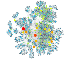
Figure 3. (a,c) Node degree distribution and (b,d) network structure for two scale-free cases with strong multifractality: (a,b) supercritical at  $\sigma = 1.82 \times 10^{-3}$ and (c,d) subcritical at $\sigma = 2.37 \times 10^{-3}$.
The structure of these scale-free networks can be visualised in figure 3(b,d): for both types of bifurcation, the low- $k$ nodes far outnumber the high- $k$ nodes. The high- $k$ nodes are known as hubs (red/orange circles), occupy the tail end of the power-law distribution, and determine the resiliency of the network (Iacobello et al. Reference Iacobello, Ridolfi and Scarsoglio2021). In turbulent flows, such hubs could represent large-scale coherent structures, whereas the low- $k$ nodes could represent small-scale vortices generated by the turbulent energy cascade (Murugesan & Sujith Reference Murugesan and Sujith2015; Taira et al. Reference Taira, Nair and Brunton2016). In our globally stable laminar jet, the hubs represent intermittent bursts of periodicity arising from coherence resonance (Zhu et al. Reference Zhu, Gupta and Li2019): the peaks of such bursts provide a clear line-of-sight to other peaks, increasing $k$. This is the origin of the observed scale-free network topology.
3.4. Early detection of global instability
Early warning indicators have been used to forewarn of impending critical transitions in various nonlinear dynamical systems (Scheffer et al. Reference Scheffer, Bascompte, Brock, Brovkin, Carpenter, Dakos, Held, Van Nes, Rietkerk and Sugihara2009). Two such indicators are  $H_2$, as computed via multifractal analysis, and the global clustering coefficient $C_g$, as computed via network analysis. The indicator $C_g$ was introduced by Watts & Strogatz (Reference Watts and Strogatz1998) to quantify the extent of node clustering in a complex network. It is defined as the number of closed triplets normalised by the total number of open and closed triplets:
 \begin{equation} C_g \equiv \frac{1}{N}\sum_{i = 1}^N {\left\{ {\left.\left( {\sum_{j,k = 1}^N {{A_{ij}}{A_{jk}}{A_{ki}}} } \right)\,\right/\left[ {{k_i}\left( {{k_i} - 1} \right)} \right]} \right\}}, \end{equation}
where  $A_{ij}$ is an edge in the adjacency matrix $\boldsymbol{\mathsf{A}}$ and $k_i = {\sum _{j = 1}^N {{A_{ij}}} }$ is the degree centrality, a measure of the number of edges incident to a given node $i$. The value of $C_g$ ranges from 0 to 1, with higher values indicating that nodes in the network tend to cluster together more tightly. Figure 4 shows the bifurcation diagrams, $H_2$ and $C_g$, all as functions of $Re$ for different values of $\sigma$. In the subcritical case (figure 4b), the bistable regime shrinks as $\sigma$ increases owing to noise-induced triggering, eventually disappearing altogether at high $\sigma$ and making the bifurcation appear supercritical.

Figure 4. Early detection of global instability: (a,b) bifurcation diagrams, (c,d) the Hurst exponent  $H_2$, and (e,f) the global clustering coefficient $C_g$, all as functions of $Re$ for different noise intensities $\sigma$. In panels (c–f), the hollow markers denote globally stable states, while the filled markers denote globally unstable states. The supercritical and subcritical cases are shown in the left and right columns, respectively.
First we consider  $H_2$. In the supercritical case (figure 4c), $H_2$ decreases gradually towards zero as $Re$ increases towards the Hopf point, indicating that the mean-reversion processes of the jet become stronger as the onset of global instability is approached. Crucially, the decrease in $H_2$ occurs well before the jet oscillation amplitude ( $|\bar {A}|$) starts to rise. This suggests that it might be possible to estimate the proximity to the supercritical Hopf point based on a calibrated $H_2$ threshold. Such a threshold, however, would depend on the noise intensity because the rate at which $H_2$ decreases with $Re$ diminishes as $\sigma$ increases. Physically this occurs because while the jet is globally stable before the Hopf point, it is still convectively unstable (Huerre & Monkewitz Reference Huerre and Monkewitz1990). Convectively unstable modes tend to spatially amplify any injected noise, at certain frequencies more than others, causing a preferred mode to emerge via coherence resonance (Zhu et al. Reference Zhu, Gupta and Li2019). Thus, somewhat counterintuitively, noise promotes order, enhancing the coherence of the jet and reducing the sensitivity of $H_2$ to $Re$. In the subcritical case (figure 4d), $H_2$ remains relatively constant at each $\sigma$ as $Re$ increases towards the Hopf point, after which $H_2$ falls sharply. This indicates that $H_2$ is not a reliable precursor of global instability arising from a subcritical Hopf bifurcation.
Next we consider  $C_g$. In the supercritical case (figure 4e), $C_g$ decreases gradually as $Re$ increases towards the Hopf point, making it another potential precursor of global instability. This decrease in $C_g$ is insensitive to $\sigma$ before the Hopf point. After the Hopf point, $C_g$ levels off as $\sigma$ increases because strong noise tends to disrupt the intrinsic periodicity of the limit-cycle oscillations, reducing the number of network links and thus increasing $C_g$ in the post-bifurcation regime. In the subcritical case (figure 4f), $C_g$ behaves like $H_2$ (figure 4d) in that it remains relatively constant as $Re$ increases towards the Hopf point, making it an ineffective precursor at low to moderate noise intensities. Only when the noise intensity is high enough ( $\sigma = 2.93 \times 10^{-3}$) to cause the hysteretic bistable regime to disappear can $C_g$ become a potential precursor.
From these observations, we propose that combining  $H_2$ and $C_g$, along with their slopes, into an integrated algorithm could lead to a systematic methodology for early detection of global instability. Our analysis shows that in the supercritical case, $\partial H_2 / \partial Re$ starts off near zero but decreases as the Hopf point is approached, particularly at low $\sigma$ (figure 4c). At the same time, $\partial C_g / \partial Re$ remains relatively constant at all $\sigma$ (figure 4e). In the subcritical case, $\partial H_2 / \partial Re$ remains relatively constant at all $\sigma$ (figure 4d), whereas $\partial C_g / \partial Re$ decreases as $\sigma$ increases (figure 4f). These differences in $\partial H_2 / \partial Re$ and $\partial C_g / \partial Re$ could be exploited to identify the bifurcation type. Once the bifurcation type is identified (and $\sigma$ is measured), $H_2$ or $C_g$ could be used as an instability precursor in the supercritical case, because both of these indicators decrease as $Re$ approaches the Hopf point, with $C_g$ benefiting from reduced sensitivity to $\sigma$. However, a calibration step would be needed to determine the critical values to which $H_2$ and $C_g$ decrease at the supercritical Hopf point. Meanwhile, $C_g$ could be used as an instability precursor in the subcritical case, but only if $\sigma$ is high. If $\sigma$ is not high, neither $H_2$ nor $C_g$ is effective in the subcritical case. Taken together, these criteria may serve as the foundation of an early detection algorithm that synergistically combines multifractal analysis and complex network analysis.
3.5. Universal scaling between  $H_2$ and $\beta$


Nearly all early warning indicators of critical transitions rely on extracting information from the noise-induced dynamics of the system (Scheffer et al. Reference Scheffer, Bascompte, Brock, Brovkin, Carpenter, Dakos, Held, Van Nes, Rietkerk and Sugihara2009). Such precursors can be classified into two types: (i) those that quantify the complexity or long-term memory of a time series; and (ii) those that quantify the degree of coherence. Prime examples of the former and latter types are, respectively,  $H_2$ (Hurst Reference Hurst1951) and the coherence factor $\beta$ (Ushakov et al. Reference Ushakov, Wünsche, Henneberger, Khovanov, Schimansky-Geier and Zaks2005; Zhu et al. Reference Zhu, Gupta and Li2019). Figure 5 shows that in the globally stable regime of the jet, before the onset of limit-cycle oscillations, an inverse power-law scaling exists between $H_2$ and $\beta$ for both supercritical and subcritical Hopf bifurcations. Using least-squares regression, we find that the scaling $H_2 \sim \beta ^{-\zeta }$ has a coefficient of determination of $R^2 = 0.92$ with $\zeta = 0.48$ in the supercritical case and $R^2 = 0.82$ with $\zeta = 0.28$ in the subcritical case. These scaling laws are independent of $Re$ and $\sigma$, giving them some degree of universality for the early detection of global instability in low-density jets.

Figure 5. Inverse power-law scaling between  $H_2$ and $\beta$ for various $\sigma$ in the globally stable regime, prior to (a) supercritical and (b) subcritical Hopf bifurcations. The error bars denote the standard deviation of $H_2$.
4. Conclusions
We have provided the first experimental evidence of multifractality and scale-free network topology in a laminar flow: a noise-perturbed low-density jet operated at a Reynolds number below the critical point of a supercritical Hopf bifurcation and below the saddle-node point of a subcritical Hopf bifurcation. We stochastically forced the jet with acoustic waves of different amplitudes  $\sigma$ and characterised its noise-induced dynamics via multifractal detrended fluctuation analysis and complex network analysis. For both supercritical and subcritical Hopf bifurcations, we found that (i) the degree of multifractality, as quantified by the width of the singularity spectrum, reaches a maximum at intermediate noise intensities; (ii) the conditions with the strongest multifractality give rise to a complex network whose node degree distribution obeys an inverse power-law scaling with an exponent of $2 < \gamma < 3$, indicating scale-free topology; and (iii) the Hurst exponent $H_2$ and the global clustering coefficient $C_g$ can serve as early warning indicators of global instability, but their effectiveness depends on the bifurcation type and the noise intensity. Specifically, we have found that both $H_2$ and $C_g$ can serve as precursors of supercritical Hopf bifurcations, especially when $\sigma$ is low. However, we also found that only $C_g$ can serve as a precursor of subcritical Hopf bifurcations, and only under specific forcing conditions: when $\sigma$ is high enough to merge the saddle-node and Hopf points, eliminating the hysteretic bistable regime. Finally, we have identified a universal power-law scaling between $H_2$ and the coherence factor $\beta$, establishing a link between fractal-based and coherence-based precursors of global instability.
Although both multifractality and scale-free network topology have previously been observed in turbulent flows, they have not been observed in a laminar flow – until now. Here we have shown that applying stochastic forcing to a laminar flow can cause it to exhibit the same type of multifractal and scale-free network dynamics usually seen in turbulent flows. This discovery supports the notion that the complex dynamics of turbulent flows can be modelled with low-order oscillators subjected to additive noise (Noiray & Schuermans Reference Noiray and Schuermans2013; Rigas et al. Reference Rigas, Morgans, Brackston and Morrison2015; Sieber et al. Reference Sieber, Paschereit and Oberleithner2021). This discovery also supports the notion that deterministic spatiotemporal chaos in hydrodynamic systems can be modelled with the Kardar–Parisi–Zhang (KPZ) equation, a nonlinear stochastic partial differential equation. Many spatiotemporally chaotic systems are known to belong to the KPZ universality class, demonstrating that the small-scale features of deterministic systems can have effects equivalent to those of a stochastic noise term (Boghosian, Chow & Hwa Reference Boghosian, Chow and Hwa1999). Further evidence to support this can be found in the shell models used by physicists to understand the complexity of turbulence (Biferale Reference Biferale2003). Shell models lack the spatial structure of turbulence, yet they retain most of the temporal complexity. These models are dimensionally consistent with the Navier–Stokes equations and can reproduce the multiscale dynamics of three-dimensional turbulence, without incorporating any geometrical complexity (Biferale Reference Biferale2003). Finally, we note that the ability of  $H_2$ and $C_g$ to forewarn of an impending critical transition to global instability could find uses in various other self-excitable flows, such as bluff-body wakes and swirling jets. The applicability of these early warning indicators to such flows remains to be explored.
Funding
This work was funded by the Research Grants Council of Hong Kong (project nos. 16200220 and 16215521). Y.G. was supported by the PolyU Start-up Fund (project no. P0043562).
Declaration of interests
The authors report no conflict of interest.


 Open access