


1. Introduction
In recent years, there has been considerable effort in providing reduced-order models that explain the dynamics of the inertial-dominated logarithmic region of high-Reynolds-number wall-bounded flows (Jiménez & Moser Reference Jiménez and Moser2007; Marusic, Mathis & Hutchins Reference Marusic, Mathis and Hutchins2010; Smits, McKeon & Marusic Reference Smits, McKeon and Marusic2011). This effort, which has been facilitated by the ubiquity of experimentally or numerically generated statistical data sets, has been motivated by the dynamic relevance of this region of wall turbulence in turbulent kinetic energy production (Smits et al. Reference Smits, McKeon and Marusic2011; Smits & Marusic Reference Smits and Marusic2013). In this vein, one of the most commonly cited models is the attached eddy model, which is based on the hypothesis that the number of attached eddies drops off at a rate that is inversely proportional to the distance from the wall (Townsend Reference Townsend1976). At the same time, the size of said eddies is assumed to grow proportionally with their wall-normal distance. Thereby, the attached eddy model provides a conceptual picture of the kinematics of wall-turbulence as a hierarchy of randomly distributed attached eddies that are geometrically self-similar and inertially dominated (Perry & Chong Reference Perry and Chong1982; Marusic & Monty Reference Marusic and Monty2019). However, wall attached eddies have been shown to exhibit both self-similar and non-self-similar geometric scaling with respect to their distance from the wall (Perry, Henbest & Chong Reference Perry, Henbest and Chong1986; Marusic & Monty Reference Marusic and Monty2019). Numerous studies have examined self-similarity trends in turbulent wall-bounded flows. These include modal decomposition techniques such as proper orthogonal decomposition (Gordeyev & Thomas Reference Gordeyev and Thomas2000; Hellström & Smits Reference Hellström and Smits2014; Karban et al. Reference Karban, Martini, Cavalieri, Lesshafft and Jordan2022), conditional sampling of instantaneous flow fields (Volino, Schultz & Pratt Reference Volino, Schultz and Pratt2003; Hwang, Lee & Sung Reference Hwang, Lee and Sung2020) and spectral coherence analysis using the results of numerical simulations (Moser, Rogers & Ewing Reference Moser, Rogers and Ewing1998; Del Álamo et al. Reference Del Álamo, Jiménez, Zandonade and Moser2004) and hot-wire measurements (Baars, Hutchins & Marusic Reference Baars, Hutchins and Marusic2017; Chandran et al. Reference Chandran, Baidya, Monty and Marusic2017; Deshpande et al. Reference Deshpande, Chandran, Monty and Marusic2020; Deshpande, Monty & Marusic Reference Deshpande, Monty and Marusic2021). While the structural simplicity afforded by the attached eddy model can be used to explain many statistical and structural features of wall-bounded turbulent flows (e.g. see de Giovanetti, Hwang & Choi Reference de Giovanetti, Hwang and Choi2016; Mouri Reference Mouri2017; Hwang & Sung Reference Hwang and Sung2018), its distinct limitations and potential refinements can guide our assessment of reduced-order models (Marusic & Monty Reference Marusic and Monty2019).
A characteristic feature of self-similar flow structures is their dominant energetic signature in the logarithmic layer (Townsend Reference Townsend1961). Because of this, self-similarity trends have been traditionally sought by studying the two-dimensional energy spectrum of the velocity field at various points within the logarithmic layer (Del Álamo et al. Reference Del Álamo, Jiménez, Zandonade and Moser2004; Chandran et al. Reference Chandran, Baidya, Monty and Marusic2017). However, the shared footprint of coexisting turbulent motions on the energy spectrum has been shown to obscure signatures of self-similar structures within the logarithmic layer. This effect is due to the lack of sufficient scale separation between viscous- and inertia-dominated motions, and is exacerbated in low-Reynolds-number flows (Perry et al. Reference Perry, Henbest and Chong1986; Perry & Marušic Reference Perry and Marušic1995; Baars & Marusic Reference Baars and Marusic2020a). On the other hand, the two-dimensional energy spectra of extremely high-Reynolds-number (e.g.  $Re_\tau =26\,000$) boundary layer flows have been shown to scale linearly over streamwise and spanwise wavelengths (Chandran et al. Reference Chandran, Baidya, Monty and Marusic2017). Instead, the correlation of the velocity field between points in the viscous near-wall and inertial regions of the flow was shown to be capable of accounting for the energetic signature of attached eddies that were self-similar (Deshpande et al. Reference Deshpande, Chandran, Monty and Marusic2020). Nevertheless, self-similarity trends were still shown to be degenerated at large wavelengths due to the effect of very large-scale structures that extend well beyond the logarithmic region (Deshpande et al. Reference Deshpande, Chandran, Monty and Marusic2020). To filter the effect of such very large-scale motions (VLSMs) and the potential footprint of non-attached eddies, Baars & Marusic (Reference Baars and Marusic2020a,Reference Baars and Marusicb) proposed a spectral decomposition technique for extracting a component of the energy spectrum that can be exclusively contributed to self-similar attached motions. Application of this technique to the energy spectrum of high-Reynolds-number boundary layer flow was shown to reveal the self-similarity of both active and inactive motions (Deshpande et al. Reference Deshpande, Monty and Marusic2021). The same work also revealed a pure $k^{-1}$-scaling (where $k$ is the horizontal wavenumber) for the one-dimensional energy spectrum associated with attached eddies that have little contribution to the formation of the Reynolds shear stress (i.e. inactive motions).
In this paper, we focus on the predictive capability of a class of reduced-order models in capturing the dominant self-similarity trends of high-Reynolds-number turbulent flows. This class of models is given by variants of the linearized Navier–Stokes (NS) equations around the turbulent mean velocity profile, which have shown promise in capturing various structural and statistical features of turbulent wall-bounded flow in addition to utility in model-based flow control. We next provide a brief overview of the historical significance of these models and summarize our contributions.
1.1. Linear analysis of turbulent wall-bounded shear flows
Linear mechanisms have been shown to play an important role in the emergence and maintenance of streamwise streaks in turbulent wall-bounded shear flows. For example, numerical simulations were used to attribute the formation of such structures to the linear amplification of eddies that interact with the background shear (Lee, Kim & Moin Reference Lee, Kim and Moin1990). Kim & Lim (Reference Kim and Lim2000) later highlighted the role of linear mechanisms in maintaining near-wall streamwise vortices. Such studies support the relevance of linear mechanisms in various stages of the self-sustaining regeneration cycle (Hamilton, Kim & Waleffe Reference Hamilton, Kim and Waleffe1995; Waleffe Reference Waleffe1997) and motivate the linear dynamical modelling of turbulent shear flows. One of such models is the linearized NS equations and its eddy-viscosity enhanced variant, which results from augmenting molecular viscosity with turbulent eddy-viscosity. These models have shown particular success in capturing the structural and statistical features of turbulent flows.
Chernyshenko & Baig (Reference Chernyshenko and Baig2005) used the linearized NS equations to predict the formation and spacing of near-wall streaks. The eddy-viscosity enhanced linearized NS equations were shown to reliably predict the length scales of the dominant near-wall motions in turbulent wall-bounded shear flows (Del Álamo & Jiménez Reference Del Álamo and Jiménez2006; Cossu, Pujals & Depardon Reference Cossu, Pujals and Depardon2009; Pujals et al. Reference Pujals, García-Villalba, Cossu and Depardon2009; Hwang & Cossu Reference Hwang and Cossu2010b). In particular, Hwang & Cossu (Reference Hwang and Cossu2010b) showed that eddy-viscosity enhancement imposes a self-similar scaling with respect to the wall-normal coordinate resulting in a plateau in the premultiplied one-dimensional energy spectrum. Moreover, the resolvent of the linearized NS operator has been used to provide insight into linear amplification mechanisms associated with critical layers and to explain the extraction of energy from the mean velocity to fluctuations (McKeon & Sharma Reference McKeon and Sharma2010; McKeon, Sharma & Jacobi Reference McKeon, Sharma and Jacobi2013; Sharma & McKeon Reference Sharma and McKeon2013). Moarref et al. (Reference Moarref, Sharma, Tropp and McKeon2013) studied the Reynolds number scaling and geometric self-similarity of the dominant resolvent modes associated with the eddy-viscosity enhanced linearized NS equations. They also showed that decomposition of the resolvent operator can provide low-order approximations of the energy spectrum of turbulent channel flow. More recently, Symon et al. (Reference Symon, Madhusudanan, Illingworth and Marusic2022) analysed the effects of the Cess eddy-viscosity profile (Cess Reference Cess1958) on the ability of the resolvent operator in predicting relevant spatiotemporal scales of the near-wall cycle. Illingworth, Monty & Marusic (Reference Illingworth, Monty and Marusic2018) used the eddy-viscosity enhanced model to develop a Kalman-based estimator of the velocity field based on observations from the wall-normal location corresponding to the maximum of streamwise streaks. Madhusudanan, Illingworth & Marusic (Reference Madhusudanan, Illingworth and Marusic2019) demonstrated the benefit of the eddy-viscosity enhancement in predicting turbulent eddies that are coherent over a significant wall-normal extent in high-Reynolds-number channel flow. They also showed that the addition of eddy-viscosity significantly improves the linear stochastic estimation of the fluctuation field in wall-parallel planes that are lower than measurements taken from the top of the logarithmic layer. Finally, we note that the eddy-viscosity enhanced linearized NS equations have also served as the basis for model-based design of passive flow control strategies in turbulent channels (Moarref & Jovanovic Reference Moarref and Jovanovic2012; Ran, Zare & Jovanović Reference Ran, Zare and Jovanović2021).
1.2. Stochastically forced linearized NS equations
The nonlinear terms in the NS equations play an important role in the growth of flow fluctuations and the transfer of energy between different spatiotemporal modes, both of which are important in transition to turbulence and in sustaining a turbulent state. However, due to their conservative nature, these terms do not contribute to the transfer of energy between the mean flow and velocity fluctuations (McComb Reference McComb1991; Durbin & Reif Reference Durbin and Reif2011). Inspired by this property, many studies have sought additive stochastic forcing of the linearized equations to model the uncertainty caused by neglecting the nonlinear terms or the impact of exogenous excitation sources and random initial conditions on the dynamics of fluctuations. These studies have focused on the modelling of various configurations and flow regimes ranging from homogeneous isotropic turbulence (Orszag Reference Orszag1970; Kraichnan Reference Kraichnan1971; Monin & Yaglom Reference Monin and Yaglom1975) to quasigeostrophic turbulence (Farrell & Ioannou Reference Farrell and Ioannou1993a, Reference Farrell and Ioannou1994; DelSole & Farrell Reference DelSole and Farrell1995) to transitional and turbulent channel flows (Farrell & Ioannou Reference Farrell and Ioannou1993b; Bamieh & Dahleh Reference Bamieh and Dahleh2001; Jovanovic & Bamieh Reference Jovanovic and Bamieh2005; Hwang & Cossu Reference Hwang and Cossu2010a,Reference Hwang and Cossub; Moarref & Jovanovic Reference Moarref and Jovanovic2012; Zare, Jovanovic & Georgiou Reference Zare, Jovanovic and Georgiou2017b; Ran et al. Reference Ran, Zare, Hack and Jovanovic2019).
The stochastically forced linearized NS were also used as part of restricted nonlinear models that aimed to generate self-sustained turbulence in Couette and Poiseuille flows (Farrell & Ioannou Reference Farrell and Ioannou2012; Constantinou et al. Reference Constantinou, Lozano-Durán, Nikolaidis, Farrell, Ioannou and Jiménez2014; Thomas et al. Reference Thomas, Lieu, Jovanovic, Farrell, Ioannou and Gayme2014). In these studies it was shown that even though turbulence could be triggered with white-in-time stochastic forcing, correct statistics could not be reproduced without accounting for the dynamics of the mean flow or without manipulation of the underlying dynamical modes (Bretheim, Meneveau & Gayme Reference Bretheim, Meneveau and Gayme2015; Thomas et al. Reference Thomas, Farrell, Ioannou and Gayme2015). This finding was in agreement with studies that suggested the deficiency of the linearized NS equations subject to white-in-time forcing in reproducing long-time averaged velocity correlations of channel flow (Farrell & Ioannou Reference Farrell and Ioannou1998; Jovanovic & Bamieh Reference Jovanovic and Bamieh2001; Hœpffner Reference Hœpffner2005). Moarref & Jovanovic (Reference Moarref and Jovanovic2012) showed that the variance of white-in-time stochastic forcing could be tuned to match the two-dimensional energy spectrum (integrated in the wall-normal dimension) of turbulent channel flow using the linearized NS equations. This choice was inspired by the observation that the second-order statistics of homogeneous isotropic turbulence can be exactly matched by white-in-time forcing with variance proportional to the turbulent energy spectrum (Moarref Reference Moarref2012).
Zare et al. (Reference Zare, Jovanovic and Georgiou2017b) exposed the limitations of white-in-time forcing models in reproducing the second-order statistics of turbulent channel flow using the linearized NS equations. To address this limitation, this study offered an optimization-based modelling framework for identifying the spectral content of coloured-in-time stochastic forcing that enables the linearized NS equations to match the second-order statistics of fully developed turbulence. It was also shown that the effect of coloured-in-time stochastic input can be equivalently interpreted as a structural perturbation of the linearized dynamical generator, with damping effects that are reminiscent of the role of eddy-viscosity. Such structural perturbations are suggestive of important state-feedback interactions that are lost through linearization and have inspired alternative problem formulations whereby dynamical feedback interactions are directly sought to reconcile partially available velocity correlations with the given linearized dynamics (Zare, Jovanovic & Georgiou Reference Zare, Jovanovic and Georgiou2016; Zare et al. Reference Zare, Mohammadi, Dhingra, Georgiou and Jovanović2020b).
1.3. Preview of the main results
Application of the modelling framework of Zare et al. (Reference Zare, Jovanovic and Georgiou2017b) to turbulent channel flow demonstrated its efficacy in capturing various structural and statistical features of the flow. For example, when trained with one-point correlations of the velocity field (normal/shear stresses), it was shown that such models not only match the one-dimensional energy spectra, but they also reasonably predict two-point velocity correlations that are, in turn, pertinent to the prediction of coherent flow structures as well as spatiotemporal features such as the power spectral density (see Zare et al. (Reference Zare, Jovanovic and Georgiou2017b) and Zare, Georgiou & Jovanovic (Reference Zare, Georgiou and Jovanovic2020a) for details). Building upon this observation, we propose the use of such data-enhanced stochastic dynamical models for the purpose of spectral coherence analysis in high-Reynolds-number wall-bounded shear flows. In particular, we demonstrate the efficacy of a model-based spectral coherence analysis for validating the structural hierarchy offered by the attached eddy model, i.e. the self-similarity of wall-coherent motions that dominate the energy of the logarithmic region of the wall.
The performance of our model-based approach relies on the predictive capability of the reduced-order models we use for coherence analysis over the wall-normal dimension. In this paper, we focus on a class of physics-based models, which are given by variants of the stochastically forced linearized NS equations around the Reynolds and Tiederman turbulent mean velocity profile (Reynolds & Tiederman Reference Reynolds and Tiederman1967), namely the original linearized NS equations and their eddy-viscosity enhanced variant subject to the scaled white-in-time forcing of Moarref & Jovanovic (Reference Moarref and Jovanovic2012), in addition to the data-enhanced linearized NS equations proposed by Zare et al. (Reference Zare, Jovanovic and Georgiou2017b). While all models are capable of reproducing the two-dimensional energy spectrum (integrated over the wall-normal dimension) in accordance with direct numerical simulations (DNS), the latter is capable of matching the normal and shear stresses (one-point velocity correlations) over all horizontal wavenumbers. Nevertheless, neither of these models are capable of matching two-point velocity correlations and their ability to partially reproduce this measure of coherence forms the basis for the analysis conducted in this paper.
Most of our discussion focuses on turbulent channel flow with  $Re_\tau =2003$, yet the methodology and analysis are applicable to more complex wall-bounded flow configurations. We form the linear coherence spectrum using the models highlighted above to examine their capability in identifying regions of the energy spectrum that are affected by self-similar wall-coherent structures. We compare and contrast the geometric scaling extracted from the results of said stochastic models with those resulting from spectral coherence analysis of DNS data. We then examine the scaling laws between the spatial length scales of such flow structures and follow the work of Baars et al. (Reference Baars, Hutchins and Marusic2017) to provide analytical expressions for the dependence of the linear coherence spectrum on the horizontal wavelengths. We show that the addition of eddy-viscosity enables the linearized NS model to capture a linear scaling trend in its coherence spectrum that is in close agreement with that of DNS.
At low to moderate Reynolds numbers, the signature of self-similar wall-coherent motions in the energy spectrum is obscured by the overlapping footprint of eddies of different size. To address this challenge, we use the decomposition technique proposed by Baars & Marusic (Reference Baars and Marusic2020a) to extract the energetic signature of dynamically dominant self-similar motions that actively contribute to turbulent transfer and the formation of the Reynolds shear stress. Our results demonstrate the benefits of coloured-in-time stochastic forcing in improving the predictions of scaling trends associated with such active motions in the logarithmic layer, thereby highlighting the importance of accounting for various second-order statistics of turbulent flows in developing model-based spectral filters.
1.4. Paper outline
The rest of our paper is organized as follows. In § 2 we introduce the stochastically forced linearized NS equations in evolution form and relate their steady-state covariance to two-point correlations of the velocity field. In § 3 we provide details of the stochastic processes that are used to generate statistically relevant velocity fields in the output of the linearized NS models. In § 4 we use two-point correlations generated by our stochastic models to construct the linear coherence spectrum and analyse the geometric scaling laws of wall-attached self-similar structures that dominate the logarithmic layer. In § 5 we use the linear coherence spectrum to decompose the one-dimensional energy spectrum into active and inactive motions and analyse their geometric scaling. Finally, in § 6 we provide a summary of our results and an outlook for future research directions.
2. Stochastically forced linearized NS equations
In this section, we introduce the linear models that we will use for analysing the geometric features of dominant coherent flow structures in high-Reynolds-number channels. These are based on two variants of the linearized NS equations subject to an additive source of excitation that triggers a statistical response from the linearized dynamics. The spectral proprieties of the said stochastic forcing will be determined in the next section.
For a channel flow of incompressible Newtonian fluid, the dynamics of the velocity and pressure fields are governed by the NS and continuity equations,
 \begin{equation} \left. \begin{gathered} \partial_t {\boldsymbol{u}}={-}\left( {\boldsymbol{u}} \boldsymbol{\cdot} \boldsymbol{\nabla} \right) {\boldsymbol{u}} -\boldsymbol{\nabla} P +\dfrac{1}{Re_\tau} \varDelta {\boldsymbol{u}},\\ 0= \boldsymbol{\nabla} \boldsymbol{\cdot} {\boldsymbol{u}}, \end{gathered} \right\} \end{equation}
where  ${\boldsymbol {u}}$ is the velocity vector, $P$ is the pressure, $\boldsymbol {\nabla }$ is the gradient operator, $\varDelta = \boldsymbol {\nabla } \boldsymbol {\cdot } \boldsymbol {\nabla }$ is the Laplacian operator and $t$ is time. The Reynolds number $Re_\tau = u_\tau h/\nu$ is defined in terms of the channel half-height $h$, kinematic viscosity $\nu$ and the friction velocity $u_\tau =\sqrt {\tau _w/\rho }$, where $\tau _w$ is the wall-shear stress (averaged over wall-parallel dimensions and time) and $\rho$ is the fluid density. By adopting the Reynolds decomposition to split the velocity and pressure fields into their time-averaged mean and fluctuating parts and linearizing the NS equations around the mean components, we arrive at the equations that govern the dynamics of velocity and pressure fluctuations,
 $$\begin{gather} {\boldsymbol{v}}_t ={-} \left( \boldsymbol{\nabla} \boldsymbol{\cdot} {{\bar{{\boldsymbol{u}}}}} \right) {\boldsymbol{v}} -\left( \boldsymbol{\nabla} \boldsymbol{\cdot} {\boldsymbol{v}} \right) {{\bar{{\boldsymbol{u}}}}} - \boldsymbol{\nabla} p +\dfrac{1}{Re_\tau} \varDelta {\boldsymbol{v}} + {\boldsymbol{d}}, \end{gather}$$
 $$\begin{gather}0= \boldsymbol{\nabla} \boldsymbol{\cdot} {\boldsymbol{v}}. \end{gather}$$
Here,  ${\bar {{\boldsymbol {u}}}}=[U(y)\ 0\ 0]^\textrm {T}$ denotes the vector of mean velocity, $p$ is the fluctuating pressure field and ${\boldsymbol {v}} = [u\ v\ w]^\textrm {T}$ is the vector of velocity fluctuations, with $u$,
$u$,  $v$ and $w$ representing the fluctuating components in the streamwise, $x$, wall-normal, $y$, and spanwise, $z$, directions, respectively. In (2.2a), ${\boldsymbol {d}}$ denotes a three-dimensional zero-mean additive stochastic forcing, which is commonly used to model the impact of exogenous excitation sources and initial conditions, or to capture the effect of nonlinearity in the NS equations.
In addition to equations (2.2), we also consider the eddy-viscosity enhanced linearized NS equations (Reynolds & Hussain Reference Reynolds and Hussain1972; Del Álamo & Jiménez Reference Del Álamo and Jiménez2006; Pujals et al. Reference Pujals, García-Villalba, Cossu and Depardon2009; Hwang & Cossu Reference Hwang and Cossu2010b),
 $$\begin{gather} {\boldsymbol{v}}_t ={-} \left( \boldsymbol{\nabla} \boldsymbol{\cdot} {\bar{{\boldsymbol{u}}}} \right) {\boldsymbol{v}} - \left( \boldsymbol{\nabla} \boldsymbol{\cdot} {\boldsymbol{v}} \right) {\bar{{\boldsymbol{u}}}} - \boldsymbol{\nabla} p + \dfrac{1}{Re_\tau} \boldsymbol{\nabla} \boldsymbol{\cdot} ((1 + \nu_T)(\boldsymbol{\nabla} {\boldsymbol{v}} + (\boldsymbol{\nabla} {\boldsymbol{v}})^{\rm T})) + {\boldsymbol{d}}, \end{gather}$$
 $$\begin{gather}0= \boldsymbol{\nabla} \boldsymbol{\cdot} {\boldsymbol{v}}, \end{gather}$$
which result from linearizing the NS equations around the turbulent mean velocity  ${\bar {{\boldsymbol {u}}}}$, and compensating for the nonlinear terms by augmenting the molecular viscosity with turbulent viscosity $\nu _T$. For turbulent viscosity in channel flow, we use the Reynolds & Tiederman (Reference Reynolds and Tiederman1967) profile,
 \begin{align} {\nu_{T}(y) = \dfrac{1}{2} \left(\left( 1+\left(\dfrac{c_2}{3}\,Re_\tau (1-y^2)(1+2y^2)(1-\exp({-(1-|y|)Re_\tau / c_1}))\right)^{2}\right)^{1/2} -1 \right)}, \end{align}
where parameters  $c_1$ and $c_2$ are selected to minimize the least squares deviation between the mean streamwise velocity obtained in experiments or simulations and the steady-state solution to the Reynolds-averaged NS equations in conjunction with the Boussinesq eddy-viscosity hypothesis obtained via the wall-normal integration of $Re_{\tau }(1-y)/(\nu _T+\nu )$ (McComb Reference McComb1991; Pope Reference Pope2000; Durbin & Reif Reference Durbin and Reif2011). Application of this least squares procedure in finding the best fit to the DNS-generated turbulent mean velocity (Del Álamo & Jiménez Reference Del Álamo and Jiménez2003; Del Álamo et al. Reference Del Álamo, Jiménez, Zandonade and Moser2004; Hoyas & Jiménez Reference Hoyas and Jiménez2006; Hoyas & Jimenez Reference Hoyas and Jimenez2008) yields $\{c_1 = 25.4, c_2 = 0.42\}$ for the turbulent channel flow with $Re_\tau =2003$ considered in this study.
Application of a standard conversion for the elimination of pressure (Schmid & Henningson Reference Schmid and Henningson2001) together with a Fourier transform in the wall-parallel directions brings the linearized equations (2.2) and (2.3) into the evolution form
 \begin{equation} \left. \begin{gathered} \boldsymbol{\varphi}_t(y,\boldsymbol{k},t) = \left[\boldsymbol{A}({\boldsymbol{k}})\, \boldsymbol{\varphi}(\boldsymbol{\cdot}\kern0.09em,\boldsymbol{k},t)\right](y) + \left[\boldsymbol{B}(\boldsymbol{k})\,{{\boldsymbol{d}}}(\boldsymbol{\cdot}\kern0.09em,\boldsymbol{k},t)\right](y),\\ {\boldsymbol{v}}(y,\boldsymbol{k},t) = \left[\boldsymbol{C}(\boldsymbol{k})\, \boldsymbol{\varphi}(\boldsymbol{\cdot}\kern0.09em,\boldsymbol{k},t)\right](y), \end{gathered} \right\} \end{equation}
where the state variable  $\boldsymbol {\varphi } = [v\ \eta ]^\textrm {T}$ contains the wall-normal velocity $v$ and vorticity $\eta = \partial _z u - \partial _x w$, $\boldsymbol {k} = [k_x\ k_z]^\textrm {T}$ is the vector of streamwise and spanwise wavenumbers, and $v(\pm 1,\boldsymbol {k}, t) = v_y(\pm 1, \boldsymbol {k}, t)=\eta (\pm 1, \boldsymbol {k}, t)=0$, which can be derived from the original no-slip and no-penetration boundary conditions on $u$,
$u$,  $v$ and $w$. Operators $\boldsymbol {B}$ and $\boldsymbol {C}$ are given by
 \begin{equation} \left. \begin{gathered} \boldsymbol{B}(\boldsymbol{k}) \mathrel{\mathop:}= \left[ \begin{array}{@{}ccc@{}} -\mathrm{i} k_x \varDelta^{{-}1} \partial_y & -k^2 \varDelta^{{-}1} & -\mathrm{i} k_z \varDelta^{{-}1} \partial_y\\ \mathrm{i} k_z & 0 & -\mathrm{i} k_x \end{array} \right] ,\\ \boldsymbol{C}(\boldsymbol{k}) \mathrel{\mathop:}= \left[ \begin{array}{@{}c@{}} \boldsymbol{C}_u \\ \boldsymbol{C}_v \\ \boldsymbol{C}_w \end{array} \right] = \dfrac{1}{{k}^2} \left[ \begin{array}{@{}cc@{}} \mathrm{i} k_x\partial_y & -\mathrm{i} k_z \\ {k}^2 & 0 \\ \mathrm{i} k_z\partial_y & \mathrm{i} k_x \end{array} \right] , \end{gathered} \right\} \end{equation}
where  $\mathrm {i}$ is the imaginary unit, $k^2 = k_x^2 + k_z^2$, and $\varDelta = \partial _y^2 - k^2$ is the Laplacian. For the original linearized NS model (2.2), operator $\boldsymbol {A}$ is given by
 \begin{equation} \left. \begin{gathered} \boldsymbol{A}(\boldsymbol{k}) = \left[ \begin{array}{@{}cc@{}} \boldsymbol{A}_{11}(\boldsymbol{k}) & 0 \\ \boldsymbol{A}_{21}(\boldsymbol{k}) & \boldsymbol{A}_{22}(\boldsymbol{k}) \end{array} \right] ,\\ \boldsymbol{A}_{11}(\boldsymbol{k})=\varDelta^{{-}1}\left(\dfrac{1}{Re_\tau}\varDelta^2+ \mathrm{i} k_x\,(U'' - U \varDelta)\right),\\ \boldsymbol{A}_{21}(\boldsymbol{k})={-}\mathrm{i} k_z\,U',\\ \boldsymbol{A}_{22}(\boldsymbol{k})=\dfrac{1}{Re_\tau} \varDelta- \mathrm{i} k_x U \end{gathered} \right\} \end{equation}
and for the eddy-viscosity enhanced linearized NS model (2.3), it is given by
 \begin{align} \left. \begin{gathered} \boldsymbol{A}(\boldsymbol{k}) = \left[ \begin{array}{@{}cc@{}} \boldsymbol{A}_{11}(\boldsymbol{k}) & 0 \\ \boldsymbol{A}_{21}(\boldsymbol{k}) & \boldsymbol{A}_{22}(\boldsymbol{k}) \end{array} \right] ,\\ \boldsymbol{A}_{11}(\boldsymbol{k}) = \varDelta^{{-}1}\left(\dfrac{1}{Re_\tau}((1+\nu_T)\varDelta^2+2\nu_T'\varDelta\,\partial_y+\nu_T''\,(\partial^2_y+k^2))+\mathrm{i} k_x\,(U''-U\varDelta)\right),\\ \boldsymbol{A}_{21}(\boldsymbol{k}) ={-}\mathrm{i} k_z\,U',\\ \boldsymbol{A}_{22}(\boldsymbol{k}) = \dfrac{1}{Re_\tau}((1+\nu_T)\varDelta+\nu_T'\partial_y)-\mathrm{i} k_x\,U. \end{gathered} \right\} \end{align}
In these operators, a prime denotes differentiation with respect to the wall-normal coordinate, and  $\varDelta ^2 = \partial _y^4 - 2k^2\partial _y^2 + k^4$.
We use a pseudospectral scheme with  $N$ Chebyshev collocation points in the wall-normal direction (Weideman & Reddy Reference Weideman and Reddy2000) to discretize the operators in the linearized equations (2.5). Moreover, we employ a change of variables to obtain a state-space representation in which the kinetic energy is determined by the Euclidean norm of the state vector (Zare et al. Reference Zare, Jovanovic and Georgiou2017b, appendix A). This yields the state-space model
 \begin{equation} \left. \begin{gathered} \dot{\boldsymbol{\psi}}(\boldsymbol{k},t) = {A(\boldsymbol{k})}\,\boldsymbol{\psi}(\boldsymbol{k},t) + B(\boldsymbol{k})\,{{\boldsymbol{d}}}(\boldsymbol{k},t),\\ {\boldsymbol{v}}(\boldsymbol{k},t) = C(\boldsymbol{k})\, \boldsymbol{\psi}(\boldsymbol{k},t), \end{gathered} \right\} \end{equation}
where  $\boldsymbol {\psi }$ and ${\boldsymbol {v}}$ are vectors with ${2N}$ and ${3N}$ complex-valued entries, respectively, and matrices $A$,
$A$,  $B$ and $C$ are discretized versions of the corresponding operators that incorporate the aforementioned change of coordinates. In statistical steady state, the second-order statistics of the state $\boldsymbol {\psi }$ and output velocity vector ${\boldsymbol {v}}$ in (2.9) are linearly related as follows:
 \begin{equation} \varPhi(\boldsymbol{k}) = C(\boldsymbol{k})\,X(\boldsymbol{k})\,C^*(\boldsymbol{k}). \end{equation}
Here,  $\varPhi (\boldsymbol {k}) = \lim _{t\to \infty } \left < {\boldsymbol {v}}(\boldsymbol {k},t)\, {\boldsymbol {v}}^*(\boldsymbol {k},t)\right >$ and $X(\boldsymbol {k}) = \lim _{t\to \infty } \left < \boldsymbol {\psi }(\boldsymbol {k},t)\, \boldsymbol {\psi }^*(\boldsymbol {k},t)\right >$ denote the covariance matrices of the velocity ${\boldsymbol {v}}$ and state $\boldsymbol {\psi }$, respectively, and $*$ denotes the complex-conjugate transpose. The two-point correlation matrix $\varPhi$ contains the normal and shear Reynolds stresses as one-point correlations along the diagonals of the submatrices of $\varPhi$, in addition to the off-diagonal two-point correlations (Moin & Moser Reference Moin and Moser1989) (see figure 1). As we discuss next, depending on the nature of the stochastic forcing ${\boldsymbol {d}}$ that is used to persistently excite the variables in (2.9), the state covariance matrix $X$ is either computed as the solution to the standard algebraic Lyapunov equation or a similar Lyapunov-like algebraic equation.

Figure 1. Structure of the output covariance matrix  $\varPhi = CXC^*$. One-point correlations of the velocity vector in the wall-normal direction are marked by the red lines.
3. Forcing models and flow statistics
In this study, we consider two types of stochastic forcing: (i) white-in-time forcing that ensures the recovery of the two-dimensional energy spectrum; and (ii) coloured-in-time forcing that ensures the recovery of both two- and one-dimensional energy spectra. As we explain next, the spectral content of both types of stochastic forcing are determined by DNS-generated second-order statistics and the latter approach relies on the stochastic dynamical modelling framework of Zare et al. (Reference Zare, Chen, Jovanovic and Georgiou2017a,Reference Zare, Jovanovic and Georgioub, Reference Zare, Georgiou and Jovanovic2020a).
3.1. Judiciously scaled white-in-time forcing
When the stochastic forcing  ${\boldsymbol {d}}$ in (2.9) is zero-mean and white-in-time the steady-state covariance $X$ can be determined as the solution to the standard algebraic Lyapunov equation (Kwakernaak & Sivan Reference Kwakernaak and Sivan1972)
 \begin{equation} A X + X A^* ={-}M. \end{equation}
Here,  $M = M^* \succeq 0$ is the covariance matrix of ${\bar {{\boldsymbol {d}}}} \mathrel {\mathop :}= B\, {\boldsymbol {d}}$, i.e. $\langle {\bar {{\boldsymbol {d}}}} (\boldsymbol {k},t_1) {\bar {{\boldsymbol {d}}}}^* (\boldsymbol {k},t_2)\rangle = M(\boldsymbol {k}) \delta (t_1 - t_2)$ and $\delta$ is the Dirac delta function. Following Moarref & Jovanovic (Reference Moarref and Jovanovic2012), we select the covariance of white-in-time forcing to guarantee equivalence between the two-dimensional energy spectrum of turbulent channel flow and the flow obtained by the linearized NS equations. This is achieved via the scaling
 \begin{equation} M(\boldsymbol{k}) = \dfrac{\bar{E}(\boldsymbol{k})}{\bar{E}_0(\boldsymbol{k})}\, M_0(\boldsymbol{k}), \end{equation}
where  $\bar {E}(\boldsymbol {k})=\int _{-1}^{1} E(y,\boldsymbol {k}) \,\mathrm {d} y$ is the two-dimensional energy spectrum of a turbulent channel flow obtained using the DNS-based energy spectrum $E(y,\boldsymbol {k})$ (Del Álamo & Jiménez Reference Del Álamo and Jiménez2003; Del Álamo et al. Reference Del Álamo, Jiménez, Zandonade and Moser2004), and $\bar {E}_0(\boldsymbol {k})$ is the energy spectrum resulting from (2.9) subject to a white-in-time forcing ${\boldsymbol {d}}$ with covariance
 \begin{equation} M_0(\boldsymbol{k}) =
\left[ \begin{array}{@{}cc@{}} E(y,\boldsymbol{k})\,I & 0 \\ 0 &
E(y,\boldsymbol{k})\,I \end{array} \right] .
\end{equation}
\begin{equation} M_0(\boldsymbol{k}) =
\left[ \begin{array}{@{}cc@{}} E(y,\boldsymbol{k})\,I & 0 \\ 0 &
E(y,\boldsymbol{k})\,I \end{array} \right] .
\end{equation}
Appendix A.1 includes a step-by-step procedure for determining white-in-time forcing  $\bar {{\boldsymbol {d}}}$ with such spectral content.
3.2. Data-driven coloured-in-time forcing
While carefully scaled white-in-time stochastic forcing can be used to match the two-dimensional energy spectrum of turbulent flow using the linearized NS dynamics, it falls short of matching turbulent velocity correlations, namely the normal and shear stress profiles (Zare et al. Reference Zare, Jovanovic and Georgiou2017b). When the stochastic forcing  ${\boldsymbol {d}}$ in (2.9) is coloured-in-time, the statistics of forcing are related to the state covariance $X$ via the Lyapunov-like equation (Georgiou Reference Georgiou2002a,Reference Georgioub)
 \begin{equation} A X + X A^* ={-}B H^* - H B^*. \end{equation}
Here,  $B$ is the input matrix that determines the preferred structure by which stochastic excitation enters the linearized evolution model and $H$ is a matrix that contains spectral information about the coloured-in-time stochastic forcing. The matrix $H$ is related to the cross-correlation between the forcing and the state in evolution model (2.9).
Following Zare et al. (Reference Zare, Jovanovic and Georgiou2017b), we select the matrices  $B$ and $H$ in (3.4) to guarantee equivalence between the one-dimensional energy spectrum of turbulent channel flow and the flow obtained via the linearized NS equations. Specifically, assuming knowledge of normal and shear Reynolds stress profiles from the result of DNS (Del Álamo & Jiménez Reference Del Álamo and Jiménez2003; Del Álamo et al. Reference Del Álamo, Jiménez, Zandonade and Moser2004), we determine the statistics of the coloured-in-time stochastic forcing in system (2.9) that reproduces the desired one-point correlations of the velocity field. Our desire to match such second-order statistics of the velocity field stems from their role in forming spectral filters that enable the extraction of geometric scaling laws for wall-coherent flow structures (§ 4) and the predominant role of self-similar motions in the production of shear stresses (§ 5). To this end, complete matrices $X$ and $Z$ are sought as solutions to the covariance completion problem
 \begin{equation} \left. \begin{aligned} \operatorname{minimize}_{X, Z} & \quad -\operatorname{log\,det}\left(X\right) \; + \; \alpha \, \| Z \|_\star\\ \operatorname{subject~to} & \quad A X + X A^* + Z = 0\\ & \quad (CXC^*)_{ij} =\varPhi_{ij}, \quad (i,j)\in \mathcal{I} \end{aligned} \right\} \end{equation}
where the dynamic matrices  $A$ and $C$ are problem data, in addition to the available entries of the output covariance matrix $\varPhi$ denoted by indices $(i,j)\in \mathcal {I}$. This convex optimization problem involves a composite objective, which provides a balance between the solution $X\succ 0$ to the maximum entropy problem and the complexity of the forcing model (see Zare et al. (Reference Zare, Chen, Jovanovic and Georgiou2017a) for additional details). The latter is accomplished by minimizing the nuclear norm $\| Z \|_\star$, which is used as a convex proxy for rank minimization (Fazel Reference Fazel2002; Recht, Fazel & Parrilo Reference Recht, Fazel and Parrilo2010), and the parameter $\alpha >0$ determines the importance of the nuclear norm regularization term. While the choice of $\alpha$ does not interfere with the feasibility of problem (3.5), it does, however, alter the quality of completion (Zare et al. Reference Zare, Jovanovic and Georgiou2017b, appendix C). Figure 2 displays perfect matching of the normal and shear stress profiles of a turbulent channel flow with $Re_\tau =2003$ for the wavenumber pair that corresponds to the peak of the premultiplied energy spectrum, i.e. $\boldsymbol {k} = (0.4,4.5)$.

Figure 2. One-point velocity correlations resulting from DNS of a channel flow with  $Re_\tau = 2003$ at $\boldsymbol {k}=(0.4,4.5)$ ${(-)}$ and from the solution to problem (3.5). (a) The normal stresses $uu$ ( $\circ$), $vv$ ( $\square$) and $ww$ ( $\triangle$); and (b) the shear stress $uv$ ( $\diamond$).
While one-point correlations are representative of the energy of fluctuations at various distances away from the wall, two-point correlations, i.e. off-diagonal entries in the covariance matrix, are indicators of the presence and spatial extent of coherent structures (Monty et al. Reference Monty, Stewart, Williams and Chong2007; Smits et al. Reference Smits, McKeon and Marusic2011). It has been shown that the solution to optimization problem (3.5) provides a reasonable recovery of two-point velocity correlations, especially for large values of the regularization parameter  $\alpha$ (see Zare et al. (Reference Zare, Jovanovic and Georgiou2017b, § 4.2)). This is in spite of the fact that only one-point correlations or diagonal entries of the submatrices in $\varPhi$ are typically provided as data in problem (3.5) and is attributed to the Lyapunov constraint, which maintains the relevance of flow physics by enforcing consistency between data and the linearized NS dynamics. The quality of completing the two-point correlation matrix is found to depend on the value of $\alpha$ in optimization problem (3.5) (Zare et al. Reference Zare, Jovanovic and Georgiou2017b, appendix C). In this paper, the choice of $\alpha =10^4$ is made to ensure good predictions of the dominant length scales of the near-wall cycle (Robinson Reference Robinson1991; Jiménez & Pinelli Reference Jiménez and Pinelli1999).
The solution to problem (3.5) can be used to construct a dynamical model for the realization of coloured-in-time stochastic input to the linearized NS equations (2.9). The class of generically minimal linear filters proposed by Zare et al. (Reference Zare, Jovanovic and Georgiou2017b, § 3.2) provide one such realization whose cascade connection with system (2.9) yields a minimal realization in the form of a parsimonious (low rank) modification to the original linearized dynamics (figure 3),
 \begin{equation} \dot{\boldsymbol{\psi}}(\boldsymbol{k},t) = \left( A(\boldsymbol{k}) - B(\boldsymbol{k})\, K(\boldsymbol{k})\right) \boldsymbol{\psi}(\boldsymbol{k},t) + B(\boldsymbol{k})\, {\boldsymbol{w}} (\boldsymbol{k},t). \end{equation}
Here,  ${\boldsymbol {w}}$ is a zero-mean white-in-time stochastic process with covariance $\varOmega$ and
 \begin{equation} K(\boldsymbol{k}) = \left(\tfrac{1}{2} \varOmega B^*(\boldsymbol{k}) - H^*(\boldsymbol{k}) \right) X^{{-}1}(\boldsymbol{k}) \end{equation}
for matrices  $B$ and $H$ that correspond to the factorization $Z = BH^* + H B^*$ (see Zare et al. (Reference Zare, Chen, Jovanovic and Georgiou2017a) for details). Appendix A.2 includes a step-by-step procedure for obtaining a state-space realization for the coloured-in-time forcing, which leads to the modified dynamics (3.6).

Figure 3. Parsimonious modifications of linearized dynamics are formed via the cascade connection of linearized dynamics with a spatiotemporal filter that is designed to account for partially available output statistics.
4. Self-similarity trends based on the coherence spectrum
As explained in the previous sections, the linearized NS equations and their data-enhanced variant provide statistical responses that are representative of the energy and structural features of various length scales of turbulent flows. In particular, model (3.6) was trained to reproduce the one-dimensional energy spectrum of the flow in addition to reasonably recover two-point velocity correlations between different wall-normal locations. In this section, we build on the latter feature and the work of Baars et al. (Reference Baars, Hutchins and Marusic2017) to study the geometric scaling of dominant flow structures resulting from three models: (i) the original linearized NS equations (2.2); (ii) the eddy-viscosity enhanced linearized NS equations (2.3); and (iii) the data-enhanced variant of model (ii) (i.e. model (3.6) with dynamic matrix  $A$ corresponding to (2.3)). In the remainder of the paper, these models will be referred to as LNS, eLNS and dLNS, respectively. We compare and contrast the deduced scaling trends with the attached eddy model and discuss its corruption by the signature of non-self-similar flow structures.
Both the one-point and two-point correlations of the streamwise velocity have been previously used to study the dominant geometric scaling of wall-turbulence (Chandran et al. Reference Chandran, Baidya, Monty and Marusic2017; Deshpande et al. Reference Deshpande, Chandran, Monty and Marusic2020). In high-Reynolds-number boundary layer flow, the two-dimensional energy spectrum has been shown to exhibit the geometric self-similarity of structures that reside in the logarithmic layer (Chandran et al. Reference Chandran, Baidya, Monty and Marusic2017). However, such geometric properties are typically obscured in the two-dimensional energy spectrum of low to moderate Reynolds number flows due to a lack of separation of scales. Instead, the two-point correlation of the velocity field, which quantifies the coherence between two wall-normal locations, can be used to isolate the influence of those energetic motions that reside in the logarithmic region and are coherent with the wall (Deshpande et al. Reference Deshpande, Chandran, Monty and Marusic2020). A normalized variant of the correlation between two wall-normal planes is given by the linear coherence spectrum (LCS) (Baars et al. Reference Baars, Hutchins and Marusic2017; Baidya et al. Reference Baidya2019),
 \begin{equation} \gamma^2({y},y_r;\boldsymbol{k}) \mathrel{\mathop:}= \dfrac{|\varPhi_{uu}({y},y_r,\boldsymbol{k})|^2}{\varPhi_{uu}({y},{y},\boldsymbol{k})\, \varPhi_{uu}(y_r,y_r,\boldsymbol{k})}, \end{equation}
where  $|\boldsymbol {\cdot }|$ is the modulus of a complex quantity, $\varPhi _{uu}$ is the two-point correlation of the streamwise velocity component $u$,
$u$,  $y_r$ is the distance of a predetermined reference point from the wall and ${y}$ denotes a second point whose wall-normal location can vary. Based on this, $0\le \gamma ^2 \le 1$, with perfect coherence ( $\gamma ^2=1$) happening when $y_r={y}$.
In the remainder of this section, we extract the geometric scaling of wall-attached eddies from the LCS resulting from the stochastic models introduced in § 3 and compare scaling laws with those extracted from a DNS-based LCS. In § 5 we extend this comparison to the efficacy of LCS-based spectral filters in extracting the portion of the energy spectrum that corresponds to motions that significantly contribute to the Reynolds shear stress. The LCS is determined in reference to the wall-normal location  $y_r^+=15$ to target wall-attached coherent motions that extend to farther layers of the wall. Prior studies have shown that wall-coherence remains largely unchanged for $0 \le y_r^+ \lesssim 15$ (Baars et al. Reference Baars, Hutchins and Marusic2017). We note that as the LCS only considers the magnitude of the two-point correlation between $y_r$ and ${y}$, any consistent stochastic phase shift between $u(y_r,\boldsymbol {k})$ and $u({y},\boldsymbol {k})$ would not be taken into account by our spectral coherence analysis. The DNS-based LCS is computed from the channel flow dataset provided by the Polytechnic University of Madrid (Vela-Martín et al. Reference Vela-martín, Encinar, García-gutiérrez and Jiménez2021). This dataset contains $1146$ time instances of the velocity extracted from a reduced grid of size $512\times 512\times 512$ that only accounts for scales that are larger than the viscous scale (Vela-Martín et al. Reference Vela-martín, Encinar, García-gutiérrez and Jiménez2021). The compressed dataset is computed from the result of DNS of a channel flow at $Re_\tau =2003$ with a computational box size of $8{\rm \pi} h\times 2h\times 3{\rm \pi} h$ in the streamwise, wall-normal and spanwise directions, covering a $2048\times 512\times 2048$ grid.
4.1. Geometric scaling of attached eddies in the vertical planes
For a turbulent channel flow with  $Re_\tau =2003$, figure 4 displays the LCS contours resulting from the LNS, eLNS and dLNS models plotted on top of the premultiplied one-dimensional energy spectra. As explained in § 3, the forcing ${\bar {{\boldsymbol {d}}}}$ (2.9) of each of the physics-based models is adjusted to ensure either the recovery of the wall-averaged two-dimensional energy spectrum (in the case of LNS and eLNS models) or the one-dimensional energy spectrum (in the case of the dLNS model). Note that matching the one-dimensional energy spectrum would yield the exact recovery of the two-dimensional energy spectrum as well. Figure 4 shows the premultiplied energy spectra in a colourmap as a function of the wall-normal coordinate and streamwise (a,c,e) and spanwise (b,d, f) wavelengths all in viscous units $y^+=Re_\tau (1+y)$, $\lambda _x^+=2{\rm \pi} Re_\tau /k_x$, and $\lambda _z^+=2{\rm \pi} Re_\tau /k_z$. In each panel, the missing dimensions have been averaged out.

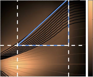
Figure 4. Contours of the LCS spectrogram obtained using the LNS (a,b), the eLNS (c,d) and the dLNS (e, f) models plotted on top of the premultiplied energy spectrum. The LCS contours are displayed as functions of the wall-normal coordinate and the streamwise (a,c,e) and spanwise (b,d, f) wavelengths all scaled in inner units. The LCS contour lines correspond to  $\{0.05:0.05:0.9\}$ coherence levels with thicker lines denoting coherence levels below $0.5$. The hypotenuse of each triangle indicates the lowest level of coherence ( $0.05$).
The LCS contour lines plotted on top of the energy spectra in figure 4 represent various levels of a coherence hierarchy predicted by the three models. While all models predict high levels of coherence in the proximity of the wall, only wall-attached eddies with large streamwise or spanwise wavelengths remain coherent in the outer layer. The elongated structures corresponding to the second energetic peak are identified by the LNS model to be weakly coherent with the wall. This is in contrast to the predictions of the eLNS and dLNS models, which predict strong coherence for large-scale structures extending beyond the logarithmic region and into the wake region in accordance with LCS-based observations made for high-Reynolds-number turbulent boundary layer flow (Baars et al. Reference Baars, Hutchins and Marusic2017).
For each of the panels in figure 4, a triangular region can be identified which is bounded from below by a wall-normal height corresponding to the shortest distinguishable geometrically self-similar eddy (or shortest height that would encompass parallel patterns within the triangle), from the left by the wavelength of the smallest inner-scaled structures, and from the right by the wavelength of the smallest distinguishable outer-scaled structures. We note that these limits are identified by visual inspection. In all spectrograms, the inner- and outer limits are marked by vertical dashed lines and the lower limits are marked by horizontal dashed lines. The hierarchies established within the triangular regions demonstrate higher levels of coherence for larger wavelengths at lower wall-normal locations, which is consistent with the additive nature of the coherence spectra of high-Reynolds-number boundary layer flows and the predictions of prior conceptual models proposed for the structure of attached eddies (Baars et al. Reference Baars, Hutchins and Marusic2017).
As indicated by the lower limit of the triangles, the initial signs of self-similar behaviour appear at  $y^+\approx 80$ from the LNS- and eLNS-based spectrograms and at $y^+\approx 100$ from the dLNS-based spectrogram. The inner limit, which indicates the smallest wall-attached wavelengths predicted by the LNS, eLNS and dLNS models, is observed at $\lambda _x/y\approx \{28,13,20\}$ and $\lambda _z/y\approx \{2.7,3,2.5\}$, respectively. Finally, the outer limit, which indicates the breakdown of self-similar scaling and the dominance of VLSMs with constant $\lambda /y$ (horizontal contours lines at large wavelengths), is predicted to happen at $\lambda _x/h\approx \{22, 22, 10\}$ and $\lambda _z/h\approx \{0.8,1.3,0.8\}$ by the LNS, eLNS and dLNS models, respectively. The extent of the self-similar region is generally in agreement with that of a turbulent boundary layer flow with $Re_\tau =2000$ extracted from the spectrogram of DNS data (Baars et al. Reference Baars, Hutchins and Marusic2017, cf. figure 4), i.e. a lower limit of $y^+\approx 80$, inner limit of $\lambda _x/y\approx 14$, and $\lambda _x/\delta \approx 10$ in the $x\unicode{x2013} y$ plane.
Within the triangles, the LCS trends are indicative of approximately self-similar flow structures with a  $y^+ \sim (\lambda _x^+)^{m_1}$ and $y^+\sim (\lambda _z^+)^{m_2}$ scaling extracted from the slope of the hypotenuse. Perfect geometric self-similarity requires $m_1=m_2=1$. The coherence contours shown in figure 4(c,e) demonstrate a $y^+ \sim (\lambda _x^+)$ and $y^+ \sim (\lambda _x^+)^{1.3}$ scaling, respectively. The same scaling laws can be deduced from figure 4(d, f), i.e. $y^+ \sim (\lambda _z^+)$ and $y^+ \sim (\lambda _z^+)^{1.3}$, respectively. These observations are indicative of perfect self-similarity of dominant wall-attached structures in the wall-parallel plane and approximate self-similarity in the $x\unicode{x2013} y$ and $y\unicode{x2013} z$ planes, with slightly better scaling laws extracted from the predictions of the eLNS model. The linear relationship between the wall-normal coordinate and horizontal wavelengths extracted from the eLNS-based LCS is in alignment with the findings of Madhusudanan et al. (Reference Madhusudanan, Illingworth and Marusic2019) and can be attributed to wall-normal scaling of the eddy-viscosity profile $\nu _T$ in the logarithmic region. On the other hand, the deviation from perfect self-similarity in the results of the dLNS model is caused by the dynamical modification affected by the coloured-in-time stochastic forcing. As described in § 3.2, this dynamical modification aims to match the two-dimensional energy spectrum at all wall-normal locations and thereby captures the energetic signature of non-self-similar motions on one-point velocity correlations that are used to compute the LCS (cf. (4.1)). In contrast to the scaling laws extracted for eLNS and dLNS models, those extracted from the coherence contours corresponding to the LNS model, i.e. $y^+ \sim (\lambda _x^+)^{0.45}$ and $y^+ \sim (\lambda _z^+)^{0.45}$, are not indicative of self-similarity (figure 4a,b). This observation, which implies that the LNS model fails to capture the coherence between the reference point $y_r$ and the logarithmic region, can be attributed to the highly localized nature of the flow structures captured by this model (Madhusudanan et al. Reference Madhusudanan, Illingworth and Marusic2019).
Based on the findings of this section, regardless of the type of additive forcing, eddy-viscosity enhanced models (eLNS and dLNS) better capture previously established geometric scaling laws of attached eddies (cf. Marusic & Monty (Reference Marusic and Monty2019)). The aforementioned imperfect self-similarity at large wavelengths can be attributed to the spectral signature of wall-coherent (i.e. wall-attached) large-scale structures that reside in the outer layer and are known to be non-self-similar (Marusic & Monty Reference Marusic and Monty2019). Such flow structures are known for actively modulating the production of near-wall scales while playing a crucial role in the redistribution of fine-scale motions throughout the turbulent boundary layer (Hutchins & Marusic Reference Hutchins and Marusic2007). In § 5, we use the LCS to filter out the signature of such very large-scale flow structures in analysing the self-similarity of wall-attached eddies in the logarithmic layer. We next validate the scaling laws extracted from figure 4 by analysing the collapse of the corresponding linear coherence spectra in scaled coordinates.
4.2. Wall-distance scaling of coherence spectra
In figure 4, the parallel coherence contours observed throughout the logarithmic region, imply three-dimensional self-similarity for a range of horizontal length scales. This also means that such geometric self-similarity can be made apparent by a wall-normal scaling of the associated coherence spectra. In other words, an LCS computed using a reference point  $y_r$ close to the wall and a target point in the logarithmic region would scale with the wall-normal distance of that target point (Madhusudanan et al. Reference Madhusudanan, Illingworth and Marusic2019). Figure 5 shows the isocontours of the LCS computed using the results of DNS and the three models discussed in the prior subsection as functions of $\lambda _x^+/y^+$ and $\lambda _z^+/y^+$ where $y^+$ corresponds to the wall-normal distance of the target point within the logarithmic layer, i.e. $2.6 \sqrt {Re_\tau }\leq y^+\leq 0.15 Re_\tau$. In agreement with trends observed for the isocontours of the DNS-based LCS, the isocontours of the LCS computed using the eLNS or dLNS models demonstrate reasonable collapse over various wall-normal locations, which is to be expected given the approximately linear relation between $y^+$ and $\lambda _x^+$ (or $\lambda _z^+$) observed in figure 4(c–f).

Figure 5. Contour level corresponding to  $\gamma ^2(y,y_r;\boldsymbol {k}) = \{0.1,0.4,0,7\}$ plotted for $y_r^+ =15$ and for different values of $y$ such that $2.6 \sqrt {Re_\tau }\leq y^+\leq 0.15 Re_\tau$ as a function of $\lambda _x^+/y^+$ and $\lambda _z^+/y^+$. The contours of LCS are generated using the results of (a) DNS, (b) the LNS model, (c) the eLNS model, (d) the dLNS models.
Figure 6 plots the isocontours of LCS as function of  $(\lambda _x^+)^m/y^+$ and $(\lambda _z^+)^m/y^+$ where $m$ corresponds to the power-law relations extracted from figure 4. While the isocontours of LCS resulting from the LNS model demonstrate an almost perfect collapse for this power-law scaling, the isocontours resulting from the other two models do not significantly change relative to those observed in figure 5, which is again due to the almost linear relation between the horizontal and vertical sizes of attached eddies. The almost perfect collapse of the LCS isocontours resulting from the eLNS model (figure 5c) indicates that this model outperforms the LNS model (figure 5b) in capturing not only the coherence of the large-scale flow structures, but also their self-similar nature (Madhusudanan et al. Reference Madhusudanan, Illingworth and Marusic2019). Interestingly, the isocontours resulting from the eLNS model demonstrate a slightly stronger collapse relative to those generated by the dLNS model (figure 6b versus figure 6c). This implies that the predictions of the dLNS model for wall-attached eddies residing in the logarithmic layer do not uniformly follow the scaling law extracted from figure 4(e, f).

Figure 6. Contour level corresponding to  $\gamma ^2(y,y_r;\boldsymbol {k}) = \{0.1,0.4,0,7\}$ plotted for $y_r^+ =15$ and for different values of $y$ such that $2.6 \sqrt {Re_\tau }\leq y^+\leq 0.15 Re_\tau$ as a function of $(\lambda _x^+)^m/y^+$ and $(\lambda _z^+)^m/y^+$ with the power $m$ corresponding to the scaling laws extracted from figure 4. The contours of LCS are generated by (a) the LNS model ( $m=0.45$), (b) the eLNS model ( $m=1$) and (c) the dLNS model ( $m=1.3$).
4.3. Analytical models for the LCS
Inspired by the collapse of coherence contours in figures 6(b) and 6(c), we propose a simplified analytical model for the dependence of the LCS corresponding to eLNS and dLNS models on the normalized horizontal wavelengths. In order to obtain the approximate model for the LCS we focus on the spectral regions corresponding to  $\gamma ^2 > 0.05$. Figure 7 shows the two-dimensional coherence spectra together with trapezoidal prisms that best approximate the LCS surfaces. The analytical expressions for the trapezoidal prisms are given by
 $$\begin{gather} \gamma^2(y^+,y_r^+ = 15; \lambda_x^+,\lambda_z^+)\nonumber\\ = \begin{cases} c_1 \log\left((\lambda_x^+)^{m}/y^+\right) + c_2 \log\left((\lambda_z^+)^{m}/y^+\right), & (\lambda_z^+)^{m}/y^+ > c_6(\lambda_x^+)^{m}/y^+\\ c_3 \log\left((\lambda_x^+)^{m}/y^+\right) + c_4 \log \left((\lambda_z^+)^{m}/y^+\right), & (\lambda_z^+)^{m}/y^+ < c_6(\lambda_x^+)^{m}/y^+\\ c_5, & (\lambda_z^+)^{m}/y^+ > b_z , (\lambda_x^+)^{m}/y^+ > b_x \end{cases} \end{gather}$$
with parameters provided in table 1. These parameters ensure a best fit using the least squares distance between the model-based LCS data and the masking planes determined by the analytical models. The spectral limits  $b_x$, and $b_z$ correspond to the edges of the plateau formed at the top of the prisms where the LCS take their maximum values (cf. figure 7a,b).

Figure 7. Two-dimensional surface plot of the LCS of turbulent channel flow at  $Re_\tau =2003$ with $y_r^+=15$ and $2.6 \sqrt {Re_\tau }\leq y^+\leq 0.15 Re_\tau$ corresponding to the (a) eLNS and (b) dLNS models. Black lines represent edges of best fit trapezoidal prisms that approximate the LCS.
Table 1. Constant parameters for the LCS model proposed in (4.2).

The LCS model in (4.2) represents a two-dimensional model-based generalization of the spectral filter proposed by Baars et al. (Reference Baars, Hutchins and Marusic2017) and Baars & Marusic (Reference Baars and Marusic2020a,Reference Baars and Marusicb) based on experimentally measured coherence levels in high-Reynolds-number boundary layer flows. The pyramid-like geometry of the fitted prisms in figure 7 imply that only large-scale structures remain coherent with the wall as the distance from the wall increases (Baars et al. Reference Baars, Hutchins and Marusic2017; Madhusudanan et al. Reference Madhusudanan, Illingworth and Marusic2019; Baars & Marusic Reference Baars and Marusic2020a). Our numerical experiments show that variations of  $y_r$ (4.1) below $y^+=15$ do not result in significant changes to the coherence spectra. The robustness of the proposed analytical LCS models in (4.2) is indicative of the strong near-wall footprint of the targeted wall-attached flow structures that dominate the logarithmic region and is in agreement with the DNS-based filter-diagnostic proposed by Baars & Marusic (Reference Baars and Marusic2020a) for a turbulent boundary layer flow with $Re_\tau =2000$.
5. Spectral filters for energy decomposition
In the previous section, we showed that the inclusion of an eddy-viscosity model can significantly improve the geometric scaling of dominant flow structures that result from the linearized NS equations. However, at low to moderate Reynolds numbers, such coherence analysis is obscured by overlapping contributions from eddies with different geometric attributes (Perry et al. Reference Perry, Henbest and Chong1986; Perry & Marušic Reference Perry and Marušic1995; Baars & Marusic Reference Baars and Marusic2020a). Herein, we adopt the spectral decomposition technique introduced by Baars & Marusic (Reference Baars and Marusic2020a) to separate the energetic signature of such overlapping length scales. This method is based on the concept of active and inactive motions that was originally introduced by Townsend (Reference Townsend1961, Reference Townsend1976).
Based on Townsend (Reference Townsend1976), active motions are a constituent part of wall turbulence that play a major role in momentum transfer and the production of Reynolds shear stress. This classification follows the significance of vortex structures with image vortex pairs in the plane of the wall that result in an impermeability boundary condition ( $v=0$) while allowing slip (finite $u$ and $w$) at the wall, and ultimately lead to a spatially localized wall-normal velocity signature (Perry & Chong Reference Perry and Chong1982, figure 2); see Deshpande et al. (Reference Deshpande, Monty and Marusic2021) for details. Consequently, at any wall-normal location $y$ within the logarithmic layer, active motions are the attached eddies with wall-normal extent ${\mathcal {H}} \sim O(y)$. Unlike active motions, inactive motions have a small contribution to Reynolds shear stress and are affected by wall-coherent structures that are much taller, and extend beyond the point of interest $y$, i.e. $O(y) \ll {\mathcal {H}} < h$ ( $h$ is the channel half-height). Based on this, the LCS (4.1) can be used to decompose the streamwise velocity spectrum $\varPhi _{uu}$ in the wall-parallel plane at $y$ into an inactive component and a residual as follows:
 $$\begin{gather} \varPhi_{ia}(y,y;\boldsymbol{k}) \mathrel{\mathop:}= \gamma^2(y,y_r;\boldsymbol{k})\, \varPhi_{uu}(y,y;\boldsymbol{k}) = \dfrac{|\varPhi_{uu}(y,y_r,\boldsymbol{k})|^2}{\varPhi_{uu}(y_r,y_r,\boldsymbol{k})}, \end{gather}$$
 $$\begin{gather}\varPhi_{a}(y,y;\boldsymbol{k}) = \varPhi_{uu}(y,y;\boldsymbol{k}) - \varPhi_{ia}(y,y;\boldsymbol{k}). \end{gather}$$
Here, the reference point  $y_r$ is chosen close to the wall to target wall-coherent flow structures and $\varPhi _{ia}(y,y;\boldsymbol {k})$ denotes the portion of the two-dimensional energy spectrum that contains the signature of attached eddies that have wall-normal extents beyond $y$. This inactive component $\varPhi _{ia}$ can alternatively be interpreted as the linear stochastic estimate of the spectrum at $y$ (see Deshpande et al. (Reference Deshpande, Monty and Marusic2021, appendix A) for details). Since we focus on evaluating the self-similarity of wall-coherent structures in the logarithmic region, we will neglect traces of non-coherent small dissipative scales in the residual energy computed in (5.1b) and assume that $\varPhi _{a}$ solely captures the signature of self-similar motions that are active. Figures 12(c,d) and 13(a,b) show the premultiplied active component of the streamwise energy spectrum $\varPhi _{a}$ and the premultiplied Reynolds shear stress cospectrum $\varPhi _{uv}$ computed using DNS data. The coinciding regions of inner-scaled wavelengths in comparing $\varPhi _{a}$ and $\varPhi _{uv}$ provide evidence that $\varPhi _{a}$ is associated with active motions of the flow. We note that the inactive component of the energy spectrum also includes contributions from wall-coherent self-similar eddies, whose signature is obscured by the presence of VLSMs that are not self-similar. At significantly higher Reynolds numbers relative to those considered in the present work, the larger wall-normal gap between the reference and target points considered in the computation of the LCS warrant a subsequent decomposition of the inactive energy component whereby the self-similar motions can be separated from the VLSMs (see Baars & Marusic (Reference Baars and Marusic2020a) for additional details).
Figure 8 depicts the premultiplied energy spectrum using inner- and outer-scaling. This figure shows that throughout the logarithmic region, small-to-medium wavelengths ( $\lambda _x^+ \lesssim 2\times 10^4$ and $\lambda _z^+ \lesssim 10^3$) scale with the distance to the wall and large wavelengths scale with the channel half-height, which is consistent with observations from turbulent boundary layer flow (Bradshaw Reference Bradshaw1967; Baidya et al. Reference Baidya, Philip, Hutchins, Monty and Marusic2017; Deshpande et al. Reference Deshpande, Chandran, Monty and Marusic2020). This distinct scaling trend hints at the potential to decompose the energy spectrum over wavelengths with exclusively inner- or outer-scaling. We thus use the spectral decomposition technique given by (5.1) to decompose the energy spectrum in the logarithmic region $116 \le y^+ \le 300$ with a concentration on wavelengths that contain at least $10\,\%$ of the energetic peak.

Figure 8. Contour lines denoting 15 % of the maximum premultiplied streamwise energy spectrum of turbulent channel flow at  $Re_\tau =2003$ evaluated over the logarithmic region ( $2.6 \sqrt {Re_\tau }\leq y^+\leq 0.15 Re_\tau$) plotted as functions of horizontal wavelengths scaled by (a) the distance from the wall and (b) the channel half-height ( $h=1$).
Figure 9(a,b) show the result of the spectral decomposition highlighted in (5.1) based on a DNS-based LCS, and figure 9(c–h) demonstrate the spectral decomposition achieved by the model-based LCS resulting from LNS (2.2), eLNS (2.3) and dLNS (3.6) models. The black contour lines in this figure correspond to  $15\,\%$ of the maximum premultiplied energy at two points in the logarithmic region ( $y^+=100$ (figure 9a,c,e,g) and ${y^+=300}$ (figure 9b,d, f,h)). Regardless of the model we use to determine the LCS, the linear decomposition technique (5.1) splits the two-dimensional energy spectrum at each wall-normal location into portions that are affected by either active or inactive motions, where inactive motions contribute to larger wavelengths and active motions contribute to small and medium-sized wavelengths. The active component of the energy (blue contours) is smaller at $y^+=100$ relative to ${y^+=300}$. This is to be expected because the number of wall-attached self-similar eddies significantly reduces as we move farther away from the wall. The LCS resulting from the eLNS and dLNS models yield inactive components (red contours) whose growth over spatial dimensions (indicated by the slope of the line passing through their ridge) deviates from that of active components (blue contours) and away from the linear growth indicated by the dashed lines. This observation, which can also be made from the result of spectral decomposition using a DNS-based LCS (figure 9a,b), is in accordance with the premise that $\varPhi _{ia}$ is due to inactive motions that are non-self-similar. On the other hand, the spectral filter resulting from the LNS model fails to appropriately decompose the energy spectrum (figure 9c,d). Moreover, application of this decomposition to the energy spectrum at $y^+=100$ yields an inactive component that maintains a similar linear growth as the active component (figure 9c). Both the LNS and eLNS models yield active components (blue contours) that exhibit residual outer-scaling for large streamwise wavelengths (figure 9c–f). On the other hand, the $\gamma ^2$ resulting from the dLNS model yields an almost perfect decomposition of the energy spectrum into components that are exclusively associated with inner- and outer-scaled eddies (figure 9g,h).

Figure 9. Contour lines denoting 15 % of the maximum premultiplied streamwise energy spectrum of turbulent channel flow at  $Re_\tau =2003$ evaluated at $y^+=100$ (a,c,e,g) and $y^+=300$ (b,d, f,h) plotted as functions of horizontal wavelengths in viscous units. Black contours denote the total energy, whereas blue and red contours denote the active and inactive components resulting from decomposition (5.1) enabled by the results of DNS (a,b), LNS (c,d), eLNS (e, f) and dLNS (g,h) models. The dashed diagonal lines demonstrate perfect geometric self-similarity in the horizontal plane ( $\lambda _x^+=\lambda _z^+$).
To evaluate the performance of the model-based LCS in decomposing the energy spectrum at various wall-normal locations, figures 10 and 11 show the active and inactive components of the energy spectra at various wall-normal locations plotted as functions of horizontal wavelengths scaled with the distance from the wall  $y$ (panels a,c,e,g) and the channel half-height $h$ (panels b,d, f,h). Figure 10(a) depicts the inner-scaling of active energy components resulting from a DNS-based spectral decomposition for the majority of the spectrum besides small wavelengths (red shaded box in figure 10a). On the other hand, the active energy components demonstrate inner-scaling over small- to medium-size wavelengths with a slight deviation from inner-scaling for the largest wavelengths (green shaded box in figure 10a). In comparison with the spectral decomposition obtained using the DNS-based LCS, the dLNS model (figure 10g) outperforms the eLNS model (figure 10e) at both ends of the spectrum; at small wavelengths ( $\lambda _x^+/y^+ \lesssim 2$) the decomposition obtained by the dLNS-based LCS shows a lack of perfect inner-scaling due to the effect of the viscous layer and at medium-size wavelengths ( $\lambda _x^+/y^+ \gtrsim 10^2$) the decomposed energy spectrum shows a slight deviation from inner-scaling, which are both in agreement with the scaling of active motions resulting from the DNS-based decomposition. This superior performance can be attributed to the fact that the coloured forcing matches the Reynolds shear stress which is directly related to the active structures by definition. Finally, as expected from the results presented in figure 9, the $\gamma ^2$ predicted by the LNS model fails to decompose the energy spectrum into components that exhibit exclusive inner- or outer-scaling (figure 10c,d).

Figure 10. Contour lines denoting 15 % of the maximum premultiplied streamwise energy spectrum corresponding to active motions in a turbulent channel flow at  $Re_\tau =2003$ evaluated over the logarithmic region ( $y^+\approx 100$, $150$, $250$ and $300$) plotted as functions of horizontal wavelengths scaled by the distance from the wall (a,c,e,g) and the channel half-height (b,d, f,h). The active components result from decomposition (5.1) enabled by the results of (a,b) DNS, (c,d) LNS, (e, f) eLNS and (g,h) dLNS models. The red and green shaded squares in (a) mark regions of deviation from inner-scaling in $\varPhi _{a}$ resulting from a DNS-based decomposition.

Figure 11. Contour lines denoting 15 % of the maximum premultiplied streamwise energy spectrum corresponding to inactive motions in a turbulent channel flow at  $Re_\tau =2003$ evaluated over the logarithmic region ( $y^+\approx 100$, $150$, $250$ and $300$) plotted as functions of horizontal wavelengths scaled by the distance from the wall (a,c,e,g) and the channel half-height (b,d, f,h). The inactive components result from decomposition (5.1) enabled by the results of (a,b) DNS, (c,d) LNS, (e, f) eLNS and (g,h) dLNS models.
The scaling trends observed for wall-distance scaling of active structures in figure 10(e,g) and outer-scaling of inactive structures in figure 11( f,h) are consistent with the scaling trends detected in figures 10(a,b) and 11(a,b) from the DNS-based decomposition. Furthermore, these scaling trends are consistent with the observations made in decomposing the energy spectrum of boundary layer flow using a data-driven LCS constructed from experimental measurements (Deshpande et al. Reference Deshpande, Monty and Marusic2021). Even though  $\varPhi _{a}$ resulting from the DNS-, eLNS- and dLNS-based decompositions exhibit an almost perfect inner-scaling (figure 10a,e,g), the inactive component $\varPhi _{ia}$ shows both inner- and outer-scaling whether the spectral decomposition is conducted using a DNS-based spectral filter or one based on the aforementioned models (figures 11a,b and 11e–h). This can be attributed to the fact that $\varPhi _{ia}(y,y;\boldsymbol {k})$ comprises contributions from attached eddies of height $O(y) \ll {\mathcal {H}} < h$ as well as outer-scaled superstructures, which is also in agreement with the results of Deshpande et al. (Reference Deshpande, Monty and Marusic2021), where both inner- and outer-scaling have been observed for the inactive component of the energy spectrum. The narrow region over which we observe wall-scaling for the inactive components (figure 11g) with $\lambda _x^+/y^+ \lesssim 10^2$ is also in alignment with the results of the same study. As expected, the resulting contour lines from the LNS model do not exhibit any sign of outer-scaling for inactive energy structures (figure 11d).
In figure 12 we study the inner-scaling of the one-dimensional energy spectrum as well as the active component resulting from DNS- and dLNS-based spectral decompositions (5.1). It is evident that the inner-scaling observed for small to medium wavelengths in figure 12(a) is due to the predominant contribution from active motions (cf. figure 12c,e). This observation is consistent with those made from the two-dimensional energy spectrum shown in figure 8 and its active component shown in figure 10(a,g). We note that the inner-scaling observed for  $y^+ \lesssim \lambda ^+ \lesssim 10 y^+$ is also consistent with observations made for high-Reynolds-number boundary layer flow (see figure 3c in Deshpande et al. (Reference Deshpande, Monty and Marusic2021)). To elucidate the dynamical relevance of the active motions, we follow Deshpande et al. (Reference Deshpande, Monty and Marusic2021) in examining the spectral distribution of the premultiplied one-dimensional $uv$-cospectrum and $vv$-spectrum within the logarithmic layer (figure 13). The $uv$-cospectra shown in figure 13(a,b) demonstrate peaks at $\lambda _x^+\sim 10 y^+$ and $\lambda _z^+ \sim 3\,y^+$, which coincide with the peak of the active component of the streamwise energy spectra resulting from the DNS-based spectral decomposition $\varPhi _{{a,dns}}$ shown in figure 12(c,d) and the dLNS-based variant $\varPhi _{a}$ shown in figure 12(e, f). This coincidence and the similar inner-scaling trends observed between the $uv$-cospectrum and the active component of the streamwise energy spectrum support the argument that $\varPhi _{{a,dns}}$ and $\varPhi _{a}$ are indeed associated with active motions that contribute to the Reynolds shear stress. A similar observation was made in the coherence analysis of boundary layer flow (Bradshaw Reference Bradshaw1967; Morrison, Subramanian & Bradshaw Reference Morrison, Subramanian and Bradshaw1992; Baidya et al. Reference Baidya, Philip, Hutchins, Monty and Marusic2017; Deshpande et al. Reference Deshpande, Monty and Marusic2021). When plotted as a function of the spanwise length scale, the DNS-generated premultiplied energy spectrum of wall-normal velocity (figure 13d) exhibits an energetic peak that coincides with that of $k_z \varPhi _{uv}(\lambda _z^+)$, $k_z \varPhi _{a,dns}(\lambda _z^+)$ and $k_z \varPhi _{a}(\lambda _z^+)$ in addition to inner-scaling. In contrast, its dependence on the streamwise wavelength does not demonstrate inner-scaling besides a narrow band around $y^+ \lesssim \lambda _x^+ \lesssim 2 y^+$ and at very large wavelengths. It also lacks a peak wavelength that coincides with the active energy component (figure 13c). The deviation from inner-scaling at small streamwise wavelengths can be attributed to the contribution of viscous dissipative scales or those that follow the scaling within the inertial subrange in accordance with the observations of Deshpande et al. (Reference Deshpande, Monty and Marusic2021).

Figure 12. (a,b) Premultiplied one-dimensional streamwise energy spectrum of turbulent channel flow with  $Re_\tau =2003$ along with its active component extracted using (c,d) the DNS-based, and (e, f) dLNS-based spectral filters as a function of streamwise (a,c,e) and spanwise (b,d, f) wavelengths normalized by the wall-normal distance. In each panel, the missing dimensions have been averaged out and different lines correspond to different target wall-normal locations $y$ within the logarithmic layer.

Figure 13. Premultiplied one-dimensional (a,b) streamwise/wall-normal cospectrum and (c,d) wall-normal spectrum of turbulent channel flow with  $Re_\tau =2003$ as a function of streamwise (a,c) and spanwise (b,d) wavelengths normalized by the wall-normal distance. Each line corresponds to a wall-normal location within the logarithmic layer.
6. Concluding remarks
In this study, we propose a model-based approach to spectral coherence analysis using variants of the stochastically forced linearized NS equations. In addition to the linearized NS dynamics around the turbulent mean velocity profiles, we consider an eddy-viscosity enhanced variant of the linearized equations in which molecular viscosity is augmented with turbulent eddy-viscosity. We excite statistical responses from the linearized dynamics using two classes of stochastic forcing: (i) a scale-dependent white-in-time stochastic forcing that reproduces the two-dimensional energy spectrum (integrated in the wall-normal direction); and (ii) a scale-dependent coloured-in-time stochastic forcing that matches the normal and shear Reynolds stress profiles and thereby reproduces the one-dimensional energy spectrum of the turbulent velocity field. We have used the resulting stochastic dynamical models to construct the coherence spectrum of a turbulent channel flow with  $Re_\tau =2003$ and examined the geometric self-similarity of wall-coherent flow structures with dominant energetic footprint in the logarithmic layer. Specifically, we have compared and contrasted the structural similarity trends predicted by each of these models against self-similarity trends extracted from DNS-based coherence spectra.
Our results show that the linearized models that benefit from eddy-viscosity enhancement or coloured-in-time forcing, which itself works as a dynamical damping (Zare et al. Reference Zare, Jovanovic and Georgiou2017b), capture self-similarity trends that are expected for the energetically dominant motions affecting the logarithmic region of the wall based on the result of DNS. This is in contrast to the original linearized NS equations, which does not capture such self-similarity. Leveraging the wall-attached property of VLSMs, we have used the DNS- and model-based LCS to decompose the energy spectrum of the flow within the logarithmic layer into components that correspond to the signatures of active and inactive motions. We have demonstrated the successful extraction of the self-similar portion of the energy spectrum using both eLNS- and dLNS-based spectral filters. In particular, the dLNS-based spectral filter extracts an active component with structural similarity trends that are in close agreement with those resulting from a DNS-based filter. Further analysis of the active component of the energy spectrum extracted by the dLNS-based filter provides evidence in support of the dynamical relevance of active motions and their contribution to the formation of the Reynolds shear stress. The inactive component of the energy spectrum is critically influenced by the footprint of VLSMs that obscure self-similarity trends in the inertially dominated region close to the wall. We note that subsequent filtering of this energy component, which would result in contributions exclusive to self-similar inactive motions and the appearance of a  $k^{-1}$-scaled spectral bandwidth in the associated one-dimensional energy spectrum (Baars & Marusic Reference Baars and Marusic2020b; Deshpande et al. Reference Deshpande, Monty and Marusic2021) requires a sufficient separation of scales that is absent at the current Reynolds number.
Inspired by our observations, we have provided analytical expressions for the two-dimensional model-based coherence spectrograms. Figures 14 and 15 show the results of spectral decomposition using the analytical expression provided for the eLNS- and dLNS-based coherence spectrograms, respectively. The inner- and outer-scaling demonstrated in these figures signify the successful separation of contributions associated with active and inactive motions, respectively. These results are in agreement with figures 10(e,g) and 11( f,h) for the model-based decomposition and support the use of analytical expressions of two-dimensional coherence spectrograms for spectral decomposition. Baars et al. (Reference Baars, Hutchins and Marusic2017) demonstrated the Reynolds number independence of the coherence spectrogram of boundary layer flow. This observation is suggestive of the potential for coherence analysis based on models that are trained using velocity correlations computed from experimental measurements or numerical simulations as it opens the door to extrapolating the parameterization of the two-dimensional coherence spectrogram to higher Reynolds numbers (beyond that of the training data set). Investigating the robustness and Reynolds number scaling of our model-based analytical expressions for the coherence spectrum calls for additional in-depth examination using data from higher-Reynolds number flows and is an ongoing research topic.

Figure 14. Contour lines denoting 15 % of the maximum premultiplied streamwise energy spectrum of a turbulent channel flow at  $Re_\tau =2003$ corresponding to (a) active motion and (b) inactive motions plotted as functions of horizontal wavelengths scaled by the distance from the wall and the channel half-height, respectively. The decomposition is achieved using the analytical eLNS-based filter (4.2) and contour lines correspond to different wall-normal locations within the logarithmic region ( $y^+\approx 100$, $150$, $250$ and $300$).

Figure 15. Contour lines denoting 15 % of the maximum premultiplied streamwise energy spectrum of a turbulent channel flow at  $Re_\tau =2003$ corresponding to (a) active motion and (b) inactive motions plotted as functions of horizontal wavelengths scaled by the distance from the wall and the channel half-height, respectively. The decomposition is achieved using the analytical dLNS-based filter (4.2) and contour lines correspond to different wall-normal locations within the logarithmic region ( $y^+\approx 100$, $150$, $250$ and $300$).
Our modelling approach is in-line with early efforts in maintaining the conservative nature of the NS equations via a balanced combination of dynamical damping and stochastic forcing (Kraichnan Reference Kraichnan1959, Reference Kraichnan1971; Orszag Reference Orszag1970; Monin & Yaglom Reference Monin and Yaglom1975). The slight benefits of the coloured-in-time stochastic forcing used in the dLNS over the eLNS model in dissecting the energy spectrum is also reminiscent of more recent studies that point to the efficacy of using scale-dependent eddy-viscosity models over invariant profiles (Gupta et al. Reference Gupta, Madhusudanan, Wan, Illingworth and Juniper2021; Symon et al. Reference Symon, Madhusudanan, Illingworth and Marusic2022). We anticipate that incorporation of more sophisticated eddy-viscosity models that may vary over different spatial scales or in different directions can potentially improve the predictive capability of spectral coherence analysis using the stochastically forced linearized NS equations.
Acknowledgements
We thank Professor A. Lozano-Durán and the Fluid Dynamics Group of the Polytechnic University of Madrid (UPM), especially Dr M.P. Encinar, for providing access to the turbulent channel flow data used in computing the DNS-based coherence spectra throughout this paper. The Texas Advanced Computing Center (TACC) at The University of Texas at Austin is acknowledged for providing computing resources.
Declaration of interests
The authors report no conflict of interest.
Appendix A. Procedure for obtaining stochastic forcing models
The two-point correlation matrix  $\varPhi _{uu}$ used for computing the LCS (4.1) corresponds to variants of the linearized NS equations (model (2.5) with dynamic generator (2.7) or (2.8)) subject to white- or coloured-in-time forcing whose parameterization follows the procedure outlined below. Note that finite-dimensional approximation of the linearized dynamics and the change of variables resulting in model (2.9) precede these steps.
A.1. White-in-time forcing using by LNS and eLNS models
For each horizontal wavenumber pair  $\boldsymbol {k}$, the white-in-time forcing that matches the two-dimensional energy spectrum resulting from DNS is obtained via the following four-step procedure:
(i) Obtain the energy spectrum $E(y,\boldsymbol {k})$ from DNS-based turbulence intensities $uu$, $vv$ and $ww$ (Del Álamo & Jiménez Reference Del Álamo and Jiménez2003; Del Álamo et al. Reference Del Álamo, Jiménez, Zandonade and Moser2004), i.e. $E(y,\boldsymbol {k}) = uu(y,\boldsymbol {k}) + vv(y,\boldsymbol {k}) + ww(y,\boldsymbol {k})$, and the two-dimensional energy spectrum $\bar {E}(\boldsymbol {k})$ via wall-normal integration of $E(y,\boldsymbol {k})$.
(ii) Construct the diagonal covariance matrix
$M_0(\boldsymbol {k})$ as shown in (3.3).(iii) Obtain the energy spectrum
$\bar {E}_0(\boldsymbol {k})$ from the solution of the Lyapunov equation
(A1)as\begin{equation} A X + X A^* ={-}M_0 \end{equation}$\bar {E}_0(\boldsymbol {k}) = {\mathrm {trace}}(X(\boldsymbol {k}))$.(iv) Having computed
$\bar {E}(\boldsymbol {k})$, $\bar {E}_0(\boldsymbol {k})$ and $M_0(\boldsymbol {k})$ from prior steps, obtain the forcing covariance $M(\boldsymbol {k})$ from (3.2).


The state covariance  $X$ used in computing the two-point correlation matrix $\varPhi _{uu}(\boldsymbol {k}) = C_u(\boldsymbol {k}) X(\boldsymbol {k}) C_u^*(\boldsymbol {k})$ can be computed by solving equation (3.1).
A.2. Coloured-in-time forcing leading to the dLNS model
For each horizontal wavenumber pair  $\boldsymbol {k}$, the coloured-in-time forcing that matches the one-dimensional energy spectrum resulting from DNS is obtained via the following four-step procedure:
(i) For
$\alpha =10^4$ and $\varPhi _{i,j}$ corresponding to the DNS-generated normal and shear stress profiles $uu$, $vv$, $ww$ and $uv$, use the customized algorithms developed in Zare et al. (Reference Zare, Chen, Jovanovic and Georgiou2017a) to solve problem (3.5) for $X$ and $Z$.(ii) Use the spectral decomposition technique in Zare et al. (Reference Zare, Chen, Jovanovic and Georgiou2017a, § III.B) to decompose matrix
$Z$ into $BH^* + HB^*$.(iii) Construct the gain matrix
$K$ using (3.7) with $\varOmega =I$, $X$ from step (i), and matrices $B$ and $H$ from step (ii).(iv) The filter dynamics
(A2)generate the coloured-in-time forcing\begin{equation} \left. \begin{gathered} \dot{\phi}(\boldsymbol{k},t) = (A(\boldsymbol{k}) - B(\boldsymbol{k})\,K(\boldsymbol{k}))\,\phi(\boldsymbol{k},t) + B(\boldsymbol{k})\,{{\boldsymbol{w}}}(\boldsymbol{k},t),\\ {\boldsymbol{d}}(\boldsymbol{k},t) ={-}K(\boldsymbol{k})\, \phi(\boldsymbol{k},t) + {\boldsymbol{w}}(\boldsymbol{k},t), \end{gathered} \right\} \end{equation}${\boldsymbol {d}}$ from white-in-time forcing ${\boldsymbol {w}}$ of covariance $\varOmega =I$ and the modified dynamics of the dLNS model are obtained as in (3.6).


The state covariance  $X$ obtained in step (i) can also be directly used to compute the two-point correlation matrix $\varPhi _{uu}(\boldsymbol {k}) = C_u(\boldsymbol {k}) X(\boldsymbol {k}) C_u^*(\boldsymbol {k})$.


 Open access