


1. Introduction
Interactions between flexible structures and high-Reynolds-number flows are ubiquitous in nature and engineering applications. The physical mechanisms that govern these fluid–structure interactions provide us with important insights into the fluid dynamics of biolocomotion. For example, fish can exploit energy from surrounding vortices and move efficiently by undulating their bodies (Triantafyllou, Triantafyllou & Yue Reference Triantafyllou, Triantafyllou and Yue2000; Gazzola, Argentina & Mahadevan Reference Gazzola, Argentina and Mahadevan2014), or synchronize their motions with the oncoming vortices (Liao et al. Reference Liao, Beal, Lauder and Triantafyllou2003). These observations have inspired engineers to design and manufacture continuously deformable robots that exhibit these behaviours (Lauder et al. Reference Lauder, Anderson, Tangorra and Madden2007; Rus & Tolley Reference Rus and Tolley2015; Li et al. Reference Li2017). Birds and other flying animals also take advantage of such mechanisms to achieve efficient locomotion. In particular, bats – one of nature's most agile fliers (Swartz et al. Reference Swartz, Groves, Kim and Walsh1996; Shyy, Berg & Ljungqvist Reference Shyy, Berg and Ljungqvist1999; Swartz et al. Reference Swartz, Iriarte-Diaz, Riskin, Tian, Song and Breuer2007; Song et al. Reference Song, Tian, Israeli, Galvao, Bishop, Swartz and Breuer2008; Cheney et al. Reference Cheney, Konow, Bearnot and Swartz2015) – can adapt to the surrounding flow conditions by deforming their thin, compliant membrane wings.
An extensible membrane is a soft material that undergoes significant stretching in a fluid flow and has negligible bending rigidity. When it is aligned with a fluid flow, the surrounding fluid forces can cause it to flutter and become unstable. Being able to predict the onset of membrane instability across parameter space, either by flutter, divergence or a combination of the two, is fundamental to a wide range of applications. Stable membranes can be used in a variety of configurations in aircraft and shape-morphing airfoils (Abdulrahim, Garcia & Lind Reference Abdulrahim, Garcia and Lind2005; Lian & Shyy Reference Lian and Shyy2005; Hu, Tamai & Murphy Reference Hu, Tamai and Murphy2008; Stanford et al. Reference Stanford, Ifju, Albertani and Shyy2008; Jaworski & Gordnier Reference Jaworski and Gordnier2012; Piquee et al. Reference Piquee, López, Breitsamter, Wüchner and Bletzinger2018; Schomberg et al. Reference Schomberg, Gerland, Liese, Wünsch and Ruetten2018; Tzezana & Breuer Reference Tzezana and Breuer2019), sails (Colgate Reference Colgate1996; Kimball Reference Kimball2009) parachutes (Pepper & Maydew Reference Pepper and Maydew1971; Stein et al. Reference Stein, Benney, Kalro, Tezduyar, Leonard and Accorsi2000) and micro-air vehicles (Lian & Shyy Reference Lian and Shyy2005). When a rigid wing moves through a flow its upper surface may experience flow separation and significant reductions in aerodynamic efficiency in both steady and unsteady flows, thus limiting the aircraft's manoeuvrability and performance. However, a flexible membrane is able to adapt quickly to unsteady airflow conditions by assuming a deformed shape that can inhibit flow separation and enhance aircraft manoeuvrability. Recent developments in membrane aerodynamics are reviewed in Lian et al. (Reference Lian, Shyy, Viieru and Zhang2003) and Tiomkin & Raveh (Reference Tiomkin and Raveh2021).
The regions in parameter space where membrane flutter occurs have been predicted by linear models that mostly assume an infinite membrane span and two-dimensional (2-D) flow. In this work we use a three-dimensional (3-D) inviscid flow model based on the vortex-lattice method to study membrane stability in the linear regime of small deflections as well as large-amplitude nonlinear membrane dynamics. We find qualitative changes in flutter behaviour in some cases due to three-dimensionality.
Only a small number of studies have considered fully coupled interactions of flexible bodies and 3-D inviscid flows. The formulation of the mechanical force balance laws and the numerical methods are more complicated in three dimensions than in two dimensions and the computational expense is much higher. Inviscid flow models such as the vortex-lattice method are widely used to model viscous high-Reynolds-number flows for aquatic and aerodynamic propulsion (Kagemoto et al. Reference Kagemoto, Wolfgang, Yue and Triantafyllou2000; Katz & Plotkin Reference Katz and Plotkin2001; Shukla & Eldredge Reference Shukla and Eldredge2007; Michelin & Llewellyn Smith Reference Michelin and Llewellyn Smith2009; Willis & Persson Reference Willis and Persson2014; Ayancik, Mivehchi & Moored Reference Ayancik, Mivehchi and Moored2022) because the computational cost is generally much lower than for direct solvers (e.g. in the case of complex and deforming body geometries, immersed-boundary, lattice-Boltzmann and deforming-mesh methods (Kim & Peskin Reference Kim and Peskin2007; Willis et al. Reference Willis, Israeli, Persson, Drela, Peraire, Swartz and Breuer2007a; Zhu et al. Reference Zhu, He, Wang, Miller, Zhang, You and Fang2011; Hoover et al. Reference Hoover, Xu, Gemmell, Colin, Costello, Dabiri and Miller2021)). In the inviscid models computational elements are distributed along surfaces rather than throughout the flow volume. However, traditional inviscid approximations of flow separation work well only in certain cases such as low-angle-of-attack airfoils where trailing-edge separation is dominant. Recently leading-edge separation has been included in such models (Pan et al. Reference Pan, Dong, Zhu and Yue2012; Ramesh et al. Reference Ramesh, Gopalarathnam, Granlund, Ol and Edwards2014).
Several recent works have studied the effect of various dimensionless control parameters such as Reynolds number, density ratio, shear modulus and aspect ratio on the flutter of one or more thin plates or flags with bending rigidity in 3-D viscous, high-Reynolds-number flows (Huang & Sung Reference Huang and Sung2010; Tian, Lu & Luo Reference Tian, Lu and Luo2012; Yu, Wang & Shao Reference Yu, Wang and Shao2012; Banerjee, Connell & Yue Reference Banerjee, Connell and Yue2015; Dong, Chen & Shi Reference Dong, Chen and Shi2016; Chen et al. Reference Chen, Ryu, Liu and Sung2020). Immersed-boundary methods were used by Tian et al. (Reference Tian, Lu and Luo2012) and Huang & Sung (Reference Huang and Sung2010). Yu et al. (Reference Yu, Wang and Shao2012) used a fictitious domain method, and Banerjee et al. (Reference Banerjee, Connell and Yue2015) used a coordinate transformation method.
Immersed-boundary methods have also been used to study a number of 3-D swimming problems, such as the self-propulsion of flapping flexible plates (Masoud & Alexeev Reference Masoud and Alexeev2010; Tang et al. Reference Tang, Huang, Gao and Lu2016), the role of active muscle contraction, passive body elasticity and fluid forces in forward swimming (Mittal et al. Reference Mittal, Dong, Bozkurttas, Najjar, Vargas and Von Loebbecke2008; Borazjani et al. Reference Borazjani, Ge, Le and Sotiropoulos2013; Hoover, Griffith & Miller Reference Hoover, Griffith and Miller2017; Dawoodian & Sau Reference Dawoodian and Sau2021; Hoover et al. Reference Hoover, Xu, Gemmell, Colin, Costello, Dabiri and Miller2021) and the propulsive forces acting on flexible fish bodies (Hoover & Tytell Reference Hoover and Tytell2020).
Boundary element methods have helped identify the effects of body kinematics on thrust production and efficiency of 3-D swimmers with non-deforming (Liu Reference Liu1996; Liu & Bose Reference Liu and Bose1997) and deforming wakes (Zhu et al. Reference Zhu, Wolfgang, Yue and Triantafyllou2002). Moored (Reference Moored2018) used a boundary element method to examine the self-propelled swimming of undulatory fins and manta rays (Fish et al. Reference Fish, Schreiber, Moored, Liu, Dong and Bart-Smith2016), and to derive 3-D heaving and pitching scaling laws (Ayancik, Fish & Moored Reference Ayancik, Fish and Moored2020; Ayancik et al. Reference Ayancik, Mivehchi and Moored2022).
In the case of membranes with negligible bending stiffness, arbitrary Lagrangian–Eulerian methods have been used to study the role of leading-edge vortices in the flutter instability (Li, Jaiman & Khoo Reference Li, Jaiman and Khoo2021) and large-amplitude dynamics, particularly at large angles of attack (Li, Law & Jaiman Reference Li, Law and Jaiman2019; Li, Jaiman & Khoo Reference Li, Jaiman and Khoo2022). Here, for simplicity, we focus on the zero-angle-of-attack case and neglect leading-edge separation.
There are relatively few studies of 3-D coupled interactions of inviscid flows and flexible bodies. Recently, Hiroaki, Hayashi & Watanabe (Reference Hiroaki, Hayashi and Watanabe2021) and Hiroaki & Watanabe (Reference Hiroaki and Watanabe2021b) used nonlinear beam theory and the vortex-lattice method to analyse the limit cycle oscillations of a rectangular plate and plate vibration under harmonic forced excitation (Hiroaki & Watanabe Reference Hiroaki and Watanabe2021a). Previously Gibbs, Wang & Dowell (Reference Gibbs, Wang and Dowell2012, Reference Gibbs IV, Wang and Dowell2015) studied the 3-D linear stability problem for a flexible plate in an inviscid flow with various boundary conditions. Tang, Dowell & Hall (Reference Tang, Dowell and Hall1999) and Tang & Dowell (Reference Tang and Dowell2001) used the method to study the stability of delta wings and rectangular plates, and Murua, Palacios & Graham (Reference Murua, Palacios and Graham2012) reviewed the vortex-lattice method in similar applications.
To our knowledge the present paper is the first 3-D study of the large-amplitude dynamics of membranes (of zero bending rigidity) in inviscid flows. Here, we use a flat-wake approximation (Kagemoto et al. Reference Kagemoto, Wolfgang, Yue and Triantafyllou2000) and find good agreement between membranes with large aspect ratio in 3-D flow and membranes in 2-D flow with wake roll-up. Computing wake roll-up with high precision in three dimensions is challenging as the vortex sheet may undergo complex twisting and shearing deformations that make meshing difficult (Feng Reference Feng2007). Fast algorithms (e.g. tree codes) for the evolution of vortex sheets in three dimensions have been developed by Kaganovskiy (Reference Kaganovskiy2006), Feng, Kaganovskiy & Krasny (Reference Feng, Kaganovskiy and Krasny2009), Lindsay & Krasny (Reference Lindsay and Krasny2001), Willis, Peraire & White (Reference Willis, Peraire and White2007b) and Sakajo (Reference Sakajo2001).
In Mavroyiakoumou & Alben (Reference Mavroyiakoumou and Alben2020) we studied the membrane dynamics in a 2-D flow, where the membrane is a 1-D curvilinear segment that undergoes large deflections. We first studied the most common endpoint conditions, ‘fixed–fixed’, in which the membrane ends were held fixed, as in most previous studies of membrane flutter (Le Maître, Huberson & De Cursi Reference Le Maître, Huberson and De Cursi1999; Sygulski Reference Sygulski2007; Tiomkin & Raveh Reference Tiomkin and Raveh2017; Nardini, Illingworth & Sandberg Reference Nardini, Illingworth and Sandberg2018). We found, surprisingly, that all unstable membranes tended to a steady shape in the large-amplitude regime, except for some cases with unrealistically large deflections. This motivated us to study a second case, ‘fixed–free’, in which the trailing edge of the membrane is free to move, but only in the direction perpendicular to the oncoming flow. This corresponds to the free-end boundary condition for a string or membrane in classical mechanics (Graff Reference Graff1975; Farlow Reference Farlow1993), where the membrane end has horizontal slope. Physically, this boundary condition means that the end slides without friction perpendicularly to the membrane's flat equilibrium state (for example, in Farlow (Reference Farlow1993) the end is attached to a frictionless, massless ring). If the membrane end is also free to move in the in-plane direction, compression develops and the problem is ill posed without a stabilizing effect such as bending rigidity, and difficult to solve computationally (Triantafyllou & Howell Reference Triantafyllou and Howell1994). Recent work has studied unsteady motions by membranes with partially free edges. In Hu et al. (Reference Hu, Tamai and Murphy2008), the authors study membrane wings with partially free trailing edges and find that trailing-edge flutter can occur when the angle of attack is relatively low. Arbós-Torrent, Ganapathisubramani & Palacios (Reference Arbós-Torrent, Ganapathisubramani and Palacios2013) found experimentally that membrane wing flutter can be enhanced by the vibrations of flexible leading- and trailing-edge supports. Partially free edges exist also in sails with tensioned cables running along the edges (Kimball Reference Kimball2009). At sufficiently low tension these edges may flutter (Colgate Reference Colgate1996). A related application is to energy harvesting by membranes mounted on tensegrity structures (networks of rigid rods and elastic fibres) and placed in fluid flows (Sunny, Sultan & Kapania Reference Sunny, Sultan and Kapania2014; Yang & Sultan Reference Yang and Sultan2016). In such cases the membrane ends have some degrees of freedom akin to the free-end boundary conditions we have defined above. Recent studies have also considered interactions of flags (Mougel & Michelin Reference Mougel and Michelin2020) and membranes (Labarbe & Kirillov Reference Labarbe and Kirillov2020, Reference Labarbe and Kirillov2022) with a free surface, including flutter behaviour.
The structure of the paper is as follows. Section 2 describes our large-amplitude membrane-vortex-sheet model. Unlike our previous work (Mavroyiakoumou & Alben Reference Mavroyiakoumou and Alben2020, Reference Mavroyiakoumou and Alben2021b,Reference Mavroyiakoumou and Albena), here, we consider a membrane surface held in a 3-D inviscid flow with 12 different sets of boundary conditions. We solve this nonlinear model using Broyden's method and an unsteady vortex-lattice algorithm. Section 3 describes the numerical method. We apply a small initial perturbation to the membrane in the direction transverse to the flow and compute the subsequent dynamics, which has large-amplitude deflections if the membrane is unstable. In § 4 we perform convergence studies and validate our model by comparing the current results with our previous 2-D studies of fixed–fixed, fixed–free and free–free membranes. Section 5 describes the computed membrane dynamics and how this varies with key parameters such as the membrane mass, pretension and stretching rigidity. We find that the membrane dynamics naturally forms four groups based on the boundary conditions at the leading and trailing edges. The 3-D dynamics differs from the 2-D dynamics in several ways: in the fixed–fixed case there are unsteady 3-D motions with varying degrees of up–down asymmetry; there are complex spanwise deformations in the 3-D free–free case and some other cases with free side edges; steady, periodic and chaotic motions appear at different parameter values, and very different midspan membrane profiles appear in three dimensions. Section 6 gives the conclusions.
2. Large-amplitude membrane-vortex-sheet model
We consider the motion of an extensible membrane held in a 3-D fluid flow with velocity  $U\hat {\boldsymbol {e}}_x$ in the far field (see figure 1). In the undeformed state the membrane is flat and parallel to the flow in the plane $z = 0$. As in Alben et al. (Reference Alben, Gorodetsky, Kim and Deegan2019), the membrane obeys linear elasticity but undergoes large deflections, so geometrically nonlinear terms enter the force expression. The membrane has a small thickness $h$ and to leading order the deformations do not vary through the thickness, so they can be described by the middle surface, midway through the thickness. The middle surface is a geometric surface, a three-component vector parametrized by two spatial coordinates and time, $\boldsymbol {r}(\alpha _1,\alpha _2,t)=(x(\alpha _1,\alpha _2,t),y(\alpha _1,\alpha _2,t),z(\alpha _1,\alpha _2,t))\in \mathbb {R}^3$, where the spatial coordinates $\alpha _1\in [-L,L]$ and $\alpha _2\in [-W/2,W/2]$ are the material coordinates, the $x$ and $y$ coordinates of each point in the initially flat state (with a uniform in-plane tension – a ‘pretension’ – applied by the boundaries).

Figure 1. Schematic diagram (in perspective view) showing a 3-D membrane (dark green surface) with fixed leading and trailing edges and free side edges. Along a free edge, points are fixed to massless rings that slide without friction along vertical poles. Here,  $U\hat {\boldsymbol {e}}_x$ is the oncoming flow velocity, $W$ is the membrane's spanwise width and $2L$ is the membrane's chord. There is also a flat vortex wake (light blue surface) that emanates from the membrane's trailing edge. In the lower portion of the figure, we also show schematically (in top view) the 12 distinct boundary conditions explored in the current work. The diagonal marks indicate a fixed (F) boundary and other boundaries are free (R). The arrows indicate the far-field flow direction which is the same for each configuration.
Each of the four membrane edges is either fixed at zero deflection or free to move in the  $z$ direction, perpendicular to the oncoming flow. Then there are $2^4 = 16$ possible boundary conditions, but since the problem is symmetrical with respect to reflection in the $x$–
$x$– $z$ plane, we only need to consider 12 distinct boundary conditions, which can be denoted: FFFF, FRFF/FFFR, FRFR, FFRF, FRRF/FFRR, FRRR, RFFF, RRFF/RFFR, RRFR, RFRF, RRRF/RFRR and RRRR (with symmetrical pairs identified). Here, F stands for a fixed edge and R stands for a free edge. The first letter in each label is the leading-edge boundary condition type and the following letters are the boundary conditions moving clockwise around the rectangular membrane looking down from larger $z$ values (bottom of figure 1), as in Gibbs et al. (Reference Gibbs IV, Wang and Dowell2015). Thus, the second and fourth letters are the side-edge boundary conditions and the third letter is the trailing-edge boundary condition. We will see in the results sections that the dynamics in the 12 cases are naturally classified into four groups, based on whether the leading and trailing edges are fixed or free. Each group is placed in one of the four coloured rectangles in the lower portion of figure 1. We present the results for each group in the four subsections of § 5.2, numbered with the numbers listed at the upper left corner of each group's rectangle in figure 1. We list the equations for three examples from the set of 12 boundary conditions (and the others are analogous)
 \begin{align} \text{FRFR:}&\quad z({-}L,\alpha_2,t)=0,\; z(L,\alpha_2,t)=0,\nonumber\\ &\quad\partial_{\alpha_2} z(\alpha_1,-W/2,t)=0,\; \partial_{\alpha_2} z(\alpha_1,W/2,t)=0,\end{align}
 \begin{align} \text{FRRR:}&\quad z({-}L,\alpha_2,t)=0,\; \partial_{\alpha_1} z(L,\alpha_2,t)=0, \nonumber\\ &\quad\partial_{\alpha_2} z(\alpha_1,-W/2,t)=0,\; \partial_{\alpha_2} z(\alpha_1,W/2,t)=0, \end{align}
 \begin{align} \text{RRRR:} &\quad \partial_{\alpha_1}z({-}L,\alpha_2,t)=0, \; \partial_{\alpha_1}z(L,\alpha_2,t)=0,\nonumber\\ &\quad\partial_{\alpha_2}z(\alpha_1,-W/2,t)=0,\; \partial_{\alpha_2}z(\alpha_1,W/2,t)=0. \end{align}
Whether the edge is fixed or free affects only the out-of-plane ( $z$-) component of the membrane motion at the edge. In all cases, no in-plane motion of the membrane edges is allowed, i.e. the $x$- and $y$-coordinates of the edges are fixed (see figure 1)
 $$\begin{gather} \text{Upstream/downstream edges:} \ \left\{x\left({\pm} L,\alpha_2,t\right)={\pm} L , \quad y\left({\pm} L,\alpha_2,t\right)=\alpha_2\right\},\quad -\frac{W}{2} \leq \alpha_2 \leq \frac{W}{2}, \end{gather}$$
 $$\begin{gather}\text{Side edges:} \ \left\{x\left(\alpha_1,\pm\frac{W}{2},t\right) = \alpha_1, \quad y\left(\alpha_1,\pm\frac{W}{2},t\right)={\pm} \frac{W}{2}\right\},\quad -L \leq \alpha_1 \leq L. \end{gather}$$
We start with the stretching energy per unit undeformed area for a thin sheet with isotropic elasticity (described in § 1 of the supplementary material available at https://doi.org/10.1017/jfm.2022.957 and Efrati, Sharon & Kupferman Reference Efrati, Sharon and Kupferman2009; Alben et al. Reference Alben, Gorodetsky, Kim and Deegan2019)
 \begin{equation} w_s=\frac{h}{2}\frac{E}{1+\nu}\left(\frac{1}{1-\nu}(\epsilon_{11}^2 +\epsilon_{22}^2)+\frac{2\nu}{1-\nu}\epsilon_{11}\epsilon_{22}+2\epsilon_{12}^2\right),\end{equation}
where  $E$ is Young's modulus, $\nu$ is Poisson's ratio, $h$ is the membrane's thickness and the strain tensor is
 \begin{equation} \epsilon_{ij}(\alpha_1,\alpha_2,t)=\bar{e}\delta_{ij} +\tfrac{1}{2}\left(\partial_{\alpha_i}\boldsymbol{r}\boldsymbol{\cdot}\partial_{\alpha_j}\boldsymbol{r}-\delta_{ij}\right). \end{equation}
Here,  $\bar {e}$ denotes a constant prestrain corresponding to the pretension applied at the boundaries and $\delta _{ij}$ is the identity tensor, with $i,j\in \{1,2\}$. We take the variation of the stretching energy
 \begin{equation} W_s = \iint w_s \,{\mathrm{d}}\alpha_1 \,{\mathrm{d}}\alpha_2 \end{equation}
with respect to the position  $\boldsymbol {r}$ to obtain the stretching force per unit material area, i.e. $-\delta w_s/\delta \boldsymbol {r}$.
Integrating by parts to move derivatives off of  $\delta \boldsymbol {r}$ terms, we obtain
 \begin{align} \delta W_s&=\frac{Eh}{1+\nu}\oint\left[ \left(\frac{1}{1-\nu}\epsilon_{11}\left(\frac{\partial\boldsymbol{r}}{\partial \alpha_1}\boldsymbol{\cdot}\delta \boldsymbol{r}\right)+\frac{\nu}{1-\nu}\epsilon_{22}\left(\frac{\partial\boldsymbol{r}}{\partial \alpha_1}\boldsymbol{\cdot}\delta \boldsymbol{r}\right)+\epsilon_{12}\left(\frac{\partial\boldsymbol{r}}{\partial \alpha_2}\boldsymbol{\cdot}\delta \boldsymbol{r}\right) \right)\upsilon_1 \right.\nonumber\\ &\quad +\left. \left( \frac{1}{1-\nu}\epsilon_{22}\left(\frac{\partial\boldsymbol{r}}{\partial \alpha_2}\boldsymbol{\cdot}\delta \boldsymbol{r}\right)+\frac{\nu}{1-\nu}\epsilon_{11}\left(\frac{\partial\boldsymbol{r}}{\partial \alpha_2}\boldsymbol{\cdot}\delta \boldsymbol{r}\right)+\epsilon_{12}\left(\frac{\partial\boldsymbol{r}}{\partial \alpha_1}\boldsymbol{\cdot}\delta \boldsymbol{r}\right) \right)\upsilon_2 \right]\,{\mathrm{d}}\sigma \nonumber\\ &\quad -\frac{Eh}{1+\nu} \iint \left[\frac{\partial}{\partial \alpha_1} \left(\frac{1}{1-\nu}\epsilon_{11}\frac{\partial\boldsymbol{r}}{\partial \alpha_1}+\frac{\nu}{1-\nu}\epsilon_{22}\frac{\partial\boldsymbol{r}}{\partial \alpha_1}+\epsilon_{12}\frac{\partial\boldsymbol{r}}{\partial \alpha_2} \right)\right. \nonumber\\ &\quad \left. +\frac{\partial}{\partial \alpha_2} \left(\frac{1}{1-\nu}\epsilon_{22}\frac{\partial\boldsymbol{r}}{\partial \alpha_2}+\frac{\nu}{1-\nu}\epsilon_{11}\frac{\partial\boldsymbol{r}}{\partial \alpha_2}+\epsilon_{12}\frac{\partial\boldsymbol{r}}{\partial \alpha_1} \right) \right]\boldsymbol{\cdot}\delta\boldsymbol{r}\,{\mathrm{d}} \alpha_1\,{\mathrm{d}} \alpha_2. \end{align}
The first integral in (2.9) can be used to obtain the free edge boundary conditions. It is a boundary integral with respect to  ${\mathrm {d}}\sigma$, arc length along the boundary in the $\alpha _1$– $\alpha _2$ plane; $(\upsilon _1,\upsilon _2)$ is the outward normal in this plane. The integrand in the second integral in (2.9) gives the stretching force per unit material area
 $$\begin{gather}
\boldsymbol{f}_s={-}\frac{\delta
w_s}{\delta\boldsymbol{r}}=\frac{Eh}{1+\nu}\left[\frac{\partial}{\partial
\alpha_1}
\left(\frac{1}{1-\nu}\epsilon_{11}\frac{\partial\boldsymbol{r}}{\partial
\alpha_1}+\frac{\nu}{1-\nu}\epsilon_{22}\frac{\partial\boldsymbol{r}}{\partial
\alpha_1}+\epsilon_{12}\frac{\partial\boldsymbol{r}}{\partial
\alpha_2} \right)\right.\nonumber\\ \left. +
\frac{\partial}{\partial
\alpha_2}\left(\frac{1}{1-\nu}\epsilon_{22}\frac{\partial\boldsymbol{r}}{\partial
\alpha_2}+\frac{\nu}{1-\nu}\epsilon_{11}\frac{\partial\boldsymbol{r}}{\partial
\alpha_2}+\epsilon_{12}\frac{\partial\boldsymbol{r}}{\partial
\alpha_1} \right) \right].
\end{gather}$$
$$\begin{gather}
\boldsymbol{f}_s={-}\frac{\delta
w_s}{\delta\boldsymbol{r}}=\frac{Eh}{1+\nu}\left[\frac{\partial}{\partial
\alpha_1}
\left(\frac{1}{1-\nu}\epsilon_{11}\frac{\partial\boldsymbol{r}}{\partial
\alpha_1}+\frac{\nu}{1-\nu}\epsilon_{22}\frac{\partial\boldsymbol{r}}{\partial
\alpha_1}+\epsilon_{12}\frac{\partial\boldsymbol{r}}{\partial
\alpha_2} \right)\right.\nonumber\\ \left. +
\frac{\partial}{\partial
\alpha_2}\left(\frac{1}{1-\nu}\epsilon_{22}\frac{\partial\boldsymbol{r}}{\partial
\alpha_2}+\frac{\nu}{1-\nu}\epsilon_{11}\frac{\partial\boldsymbol{r}}{\partial
\alpha_2}+\epsilon_{12}\frac{\partial\boldsymbol{r}}{\partial
\alpha_1} \right) \right].
\end{gather}$$
The membrane dynamics is governed by the balance of momentum for a small material element with area  $\Delta \alpha _1\Delta \alpha _2$
 \begin{equation} \rho_s h\Delta \alpha_1\Delta \alpha_2\partial_{tt}\boldsymbol{r}=\boldsymbol{f}_s\Delta \alpha_1\Delta \alpha_2-[p](\alpha_1,\alpha_2,t)\boldsymbol{\hat{n}}\sqrt{\det[\partial_{\alpha_i}\boldsymbol{r}\boldsymbol{\cdot}\partial_{\alpha_j}\boldsymbol{r}]}\Delta \alpha_1\Delta \alpha_2,\end{equation}
where  $\rho _s$ is the mass per unit volume of the membrane, uniform in the undeformed state; $[p](\alpha _1,\alpha _2,t)$ is the fluid pressure; $\boldsymbol {\hat {n}}$ is the unit normal vector,
 \begin{equation} \boldsymbol{\hat{n}}=(\partial_{\alpha_1}\boldsymbol{r}\times\partial_{\alpha_2}\boldsymbol{r})/\|\partial_{\alpha_1}\boldsymbol{r}\times\partial_{\alpha_2} \boldsymbol{r}\|,\end{equation}
and  $\det [\partial _{\alpha _i}\boldsymbol {r}\boldsymbol {\cdot }\partial _{\alpha _j}\boldsymbol {r}]$ is the determinant of the metric tensor, so $\sqrt {\det [\partial _{\alpha _i}\boldsymbol {r}\boldsymbol {\cdot }\partial _{\alpha _j}\boldsymbol {r}]}\Delta \alpha _1\Delta \alpha _2$ is the area of the material element in physical space.
We non-dimensionalize the governing equations by the density of the fluid  $\rho _f$, the half-chord $L$ and the imposed fluid flow velocity $U$. The dimensionless time, space, and pressure jump variables (denoted by tildes) are
 \begin{equation} \tilde{t}=\frac{t}{L/U}, \quad(\tilde{\boldsymbol{r}},\widetilde{\alpha_1},\widetilde{\alpha_2})=\frac{(\boldsymbol{r},\alpha_1,\alpha_2)}{L},\quad\widetilde{[p]}=\frac{[p]}{\rho_fU^2}. \end{equation}
The membrane equation (2.11) becomes
 \begin{align} \frac{\rho_s
hU^2}{L}\widetilde{\partial_{tt}\boldsymbol{r}}=
\frac{Eh}{L(1+\nu)}&\left[\widetilde{\partial_{\alpha_1}}
\left(\frac{1}{1-\nu}\widetilde{\epsilon_{11}}\widetilde{\partial_{\alpha_1}\boldsymbol{r}}+\frac{\nu}{1-\nu}\widetilde{\epsilon_{22}}\widetilde{\partial_{
\alpha_1}\boldsymbol{r}}+\widetilde{\epsilon_{12}}\widetilde{\partial_{\alpha_2}\boldsymbol{r}}
\right)\right. \nonumber\\ &\left.+
\widetilde{\partial_{
\alpha_2}}\left(\frac{1}{1-\nu}\widetilde{\epsilon_{22}}\widetilde{\partial_{\alpha_2}\boldsymbol{r}}+\frac{\nu}{1-\nu}\widetilde{\epsilon_{11}}\widetilde{\partial_{\alpha_2}\boldsymbol{r}}+\widetilde{\epsilon_{12}}\widetilde{\partial_{\alpha_1}\boldsymbol{r}}
\right) \right]\nonumber\\ &
-\rho_fU^2\widetilde{[p]}\boldsymbol{\hat{n}}\sqrt{\det[\widetilde{\partial_{\alpha_i}\boldsymbol{r}}\boldsymbol{\cdot}\widetilde{\partial_{\alpha_j}\boldsymbol{r}}]}.
\end{align}
\begin{align} \frac{\rho_s
hU^2}{L}\widetilde{\partial_{tt}\boldsymbol{r}}=
\frac{Eh}{L(1+\nu)}&\left[\widetilde{\partial_{\alpha_1}}
\left(\frac{1}{1-\nu}\widetilde{\epsilon_{11}}\widetilde{\partial_{\alpha_1}\boldsymbol{r}}+\frac{\nu}{1-\nu}\widetilde{\epsilon_{22}}\widetilde{\partial_{
\alpha_1}\boldsymbol{r}}+\widetilde{\epsilon_{12}}\widetilde{\partial_{\alpha_2}\boldsymbol{r}}
\right)\right. \nonumber\\ &\left.+
\widetilde{\partial_{
\alpha_2}}\left(\frac{1}{1-\nu}\widetilde{\epsilon_{22}}\widetilde{\partial_{\alpha_2}\boldsymbol{r}}+\frac{\nu}{1-\nu}\widetilde{\epsilon_{11}}\widetilde{\partial_{\alpha_2}\boldsymbol{r}}+\widetilde{\epsilon_{12}}\widetilde{\partial_{\alpha_1}\boldsymbol{r}}
\right) \right]\nonumber\\ &
-\rho_fU^2\widetilde{[p]}\boldsymbol{\hat{n}}\sqrt{\det[\widetilde{\partial_{\alpha_i}\boldsymbol{r}}\boldsymbol{\cdot}\widetilde{\partial_{\alpha_j}\boldsymbol{r}}]}.
\end{align}
Dividing (2.14) by  $\rho _fU^2$ throughout yields
 \begin{align} \frac{\rho_s h}{\rho_f
L}\widetilde{\partial_{tt}\boldsymbol{r}}=
\frac{Eh}{\rho_fU^2L(1+\nu)}&\left[\widetilde{\partial_{\alpha_1}}
\left(\frac{1}{1-\nu}\widetilde{\epsilon_{11}}\widetilde{\partial_{\alpha_1}\boldsymbol{r}}+\frac{\nu}{1-\nu}\widetilde{\epsilon_{22}}\widetilde{\partial_{
\alpha_1}\boldsymbol{r}}+\widetilde{\epsilon_{12}}\widetilde{\partial_{\alpha_2}\boldsymbol{r}}
\right) \right.\nonumber\\ &\left.+
\widetilde{\partial_{
\alpha_2}}\left(\frac{1}{1-\nu}\widetilde{\epsilon_{22}}\widetilde{\partial_{\alpha_2}\boldsymbol{r}}+\frac{\nu}{1-\nu}\widetilde{\epsilon_{11}}\widetilde{\partial_{\alpha_2}\boldsymbol{r}}+\widetilde{\epsilon_{12}}\widetilde{\partial_{\alpha_1}\boldsymbol{r}}
\right) \right]\nonumber\\ &
-\widetilde{[p]}\boldsymbol{\hat{n}}\sqrt{\det[\widetilde{\partial_{\alpha_i}\boldsymbol{r}}\boldsymbol{\cdot}\widetilde{\partial_{\alpha_j}\boldsymbol{r}}]}.
\end{align}
\begin{align} \frac{\rho_s h}{\rho_f
L}\widetilde{\partial_{tt}\boldsymbol{r}}=
\frac{Eh}{\rho_fU^2L(1+\nu)}&\left[\widetilde{\partial_{\alpha_1}}
\left(\frac{1}{1-\nu}\widetilde{\epsilon_{11}}\widetilde{\partial_{\alpha_1}\boldsymbol{r}}+\frac{\nu}{1-\nu}\widetilde{\epsilon_{22}}\widetilde{\partial_{
\alpha_1}\boldsymbol{r}}+\widetilde{\epsilon_{12}}\widetilde{\partial_{\alpha_2}\boldsymbol{r}}
\right) \right.\nonumber\\ &\left.+
\widetilde{\partial_{
\alpha_2}}\left(\frac{1}{1-\nu}\widetilde{\epsilon_{22}}\widetilde{\partial_{\alpha_2}\boldsymbol{r}}+\frac{\nu}{1-\nu}\widetilde{\epsilon_{11}}\widetilde{\partial_{\alpha_2}\boldsymbol{r}}+\widetilde{\epsilon_{12}}\widetilde{\partial_{\alpha_1}\boldsymbol{r}}
\right) \right]\nonumber\\ &
-\widetilde{[p]}\boldsymbol{\hat{n}}\sqrt{\det[\widetilde{\partial_{\alpha_i}\boldsymbol{r}}\boldsymbol{\cdot}\widetilde{\partial_{\alpha_j}\boldsymbol{r}}]}.
\end{align}
Thus, the dimensionless membrane equation (dropping tildes) is
 \begin{align} R_1{\partial_{tt}\boldsymbol{r}}- K_s\left\{{\partial_{\alpha_1}} \left({\epsilon_{11}}{\partial_{\alpha_1}\boldsymbol{r}}+{\nu}{\epsilon_{22}}{\partial_{ \alpha_1}\boldsymbol{r}}+(1-\nu){\epsilon_{12}}{\partial_{\alpha_2}\boldsymbol{r}} \right)\right.\nonumber\\ +\left. {\partial_{ \alpha_2}}\left({\epsilon_{22}}{\partial_{\alpha_2}\boldsymbol{r}}+{\nu}{\epsilon_{11}}{\partial_{\alpha_2}\boldsymbol{r}}+(1-\nu){\epsilon_{12}}{\partial_{\alpha_1}\boldsymbol{r}} \right) \right\}\nonumber\\ ={-}{[p]}\boldsymbol{\hat{n}}\sqrt{(\partial_{\alpha_1}\boldsymbol{r}\boldsymbol{\cdot} \partial_{\alpha_1}\boldsymbol{r})(\partial_{\alpha_2}\boldsymbol{r}\boldsymbol{\cdot} \partial_{\alpha_2}\boldsymbol{r})-(\partial_{\alpha_1}\boldsymbol{r}\boldsymbol{\cdot} \partial_{\alpha_2}\boldsymbol{r})^2}, \end{align}
where  $R_1=\rho _s h/(\rho _f L)$ is the dimensionless membrane mass density, $K_s=R_3/(1-\nu ^2)$ is a dimensionless stretching stiffness written in terms of $R_3 = Eh/(\rho _fU^2L)$, the dimensionless stretching rigidity, and we have written out the determinant under the square root explicitly in (2.16). The prestrain $\bar {e}$ in (2.7) is the strain in a membrane under uniform tension $T_0 = K_s\bar {e}$, the ‘pretension’, one of the main control parameters here, as in our 2-D study (Mavroyiakoumou & Alben Reference Mavroyiakoumou and Alben2020). We assume that the thickness ratio $h/L$ is small, but $\rho _s/\rho _f$ may be large, so $R_1$ may assume any non-negative value. As in Mavroyiakoumou & Alben (Reference Mavroyiakoumou and Alben2020), we have neglected bending rigidity, denoted as $R_2$ in Alben & Shelley (Reference Alben and Shelley2008). In the extensible regime studied here, $R_3$ is finite, so $R_2=R_3h^2/(12L^2)\to 0$ in the limit $h/L\to 0$. For simplicity and for ease of comparison with the 2-D case we set the Poisson ratio $\nu$ (the transverse contraction due to axial stretching) to zero. A simple estimate of the maximum tension induced by viscous stresses is provided by the viscous drag on a flat plate, $2.66 Re^{-1/2}$ in the present non-dimensionalization (Batchelor Reference Batchelor1967), which ranges from $10^{-2.6}$ to $10^{-1.1}$ for $Re$ (the Reynolds number) in the range $10^3$– $10^6$. In this work the pretension ranges from $10^{-1.5}$ to $10^2$, but is usually at or above $10^{-1}$, so in a large number of cases the viscosity-induced tension is negligible. Therefore, to limit the number of cases under discussion, we neglect the effect of viscosity.
We solve for the flow using the vortex-lattice method, a type of panel method (Katz & Plotkin Reference Katz and Plotkin2001) that solves for the 3-D inviscid flow past a thin body by posing a vortex sheet on the body to satisfy the no-flow-through or kinematic condition. The vortex sheet is advected into the fluid at the body's trailing edge, thus avoiding a flow singularity there (Katz & Plotkin Reference Katz and Plotkin2001). The velocity  $\boldsymbol {u}$ is a uniform background flow $\hat {\boldsymbol {e}}_x$ plus the flow induced by a distribution of vorticity $\boldsymbol {\omega }$, via the Biot–Savart law (Saffman Reference Saffman1992)
 \begin{equation} \boldsymbol{u}(\boldsymbol{x})=\hat{\boldsymbol{e}}_x+\frac{1}{4{\rm \pi}}\iiint_{\mathbb{R}^3} \boldsymbol{\omega}(\boldsymbol{x}',t) \times (\boldsymbol{x}-\boldsymbol{x}')/\|\boldsymbol{x} -\boldsymbol{x}'\|^3 \,{\mathrm{d}}\boldsymbol{x}'. \end{equation}
The vorticity is a vortex sheet on the body and wake. With the body surface parametrized by  $\alpha _1$ and $\alpha _2$, we define a local coordinate basis by $\{\boldsymbol {\hat {s}}_1, \boldsymbol {\hat {s}}_2, \boldsymbol {\hat {n}}\}$
 \begin{equation} \boldsymbol{\hat{s}}_1=\frac{\partial_{\alpha_1}\boldsymbol{r}}{\|\partial_{\alpha_1}\boldsymbol{r}\|};\quad \boldsymbol{\hat{s}}_2=\frac{\partial_{\alpha_2}\boldsymbol{r}}{\|\partial_{\alpha_2}\boldsymbol{r}\|};\quad \boldsymbol{\hat{n}}\quad \text{from (2.12)}. \end{equation}
Thus,  $\boldsymbol {\hat {s}}_1$ and $\boldsymbol {\hat {s}}_2$ span the body's local tangent plane and $\boldsymbol {\hat {n}}$ is its normal vector. Here, $\boldsymbol {\hat {s}}_1$ and $\boldsymbol {\hat {s}}_2$ are also the tangents to the material lines $\alpha _2=\mathrm {constant}$ and $\alpha _1=\mathrm {constant}$, respectively. When the body experiences in-plane shear, $\boldsymbol {\hat {s}}_1$ and $\boldsymbol {\hat {s}}_2$ are not orthogonal, but they do not become parallel except for singular deformations that we do not consider.
For the vortex sheet on the body, the vorticity takes the form  $\boldsymbol {\omega }(\boldsymbol {x},t) = \boldsymbol {\gamma }(\alpha _1,\alpha _2,t)\delta (n) = \gamma _1(\alpha _1,\alpha _2,t)\delta (n)\boldsymbol {\hat {s}}_1+\gamma _2(\alpha _1,\alpha _2,t)\delta (n) \boldsymbol {\hat {s}}_2$, with $\delta (n)$ the Dirac delta distribution and $n$ the signed distance from the vortex sheet along the sheet normal. The vorticity is concentrated at the vortex sheet, $n = 0$, and $\boldsymbol {\gamma }$ is the jump in the tangential flow velocity across the vortex sheet (Saffman Reference Saffman1992). The vorticity can be written similarly in the wake vortex sheet, but a different parametrization is used since $\alpha _1$ and $\alpha _2$ are only defined on the body. The nonlinear kinematic equation states that the normal component of the body velocity equals that of the flow velocity at the body (Saffman Reference Saffman1992)
where  $S_B$ and $S_W$ are the body and wake surfaces, respectively. Since $\boldsymbol {r}$ and $\boldsymbol {x'}$ lie on $S_B$, the integral in (
) is singular, defined as a principal value integral.
The pressure jump across the membrane  $[p](\alpha _1,\alpha _2,t)$ can be written in terms of the vortex-sheet strength components $\gamma _1$ and $\gamma _2$ using the unsteady Bernoulli equation written at a fixed material point on the membrane. The formula and its derivation are lengthy so they are given in § 2 of the supplementary material, but the form of the pressure jump formula is
 \begin{equation} \partial_{\alpha_{1}}[p] = G(\boldsymbol{r},\gamma_1,\gamma_2,\mu_1,\mu_2,\tau_1,\tau_2,\nu_v). \end{equation}
Here,  $\mu _1$ and $\mu _2$ are the tangential components of the average of the flow velocity on the two sides of the membrane, i.e. the dot products of $\boldsymbol {\hat {s}}_1$ and $\boldsymbol {\hat {s}}_2$ with the term in parentheses on the right-hand side of (2.19). Also, $\tau _1$, $\tau _2$ and $\nu _v$ are the components of the membrane's velocity in the $\{\boldsymbol {\hat {s}}_1, \boldsymbol {\hat {s}}_2, \boldsymbol {\hat {n}}\}$ basis
 \begin{equation} \tau_1(\alpha_1,\alpha_2,t)=\partial_t\boldsymbol{r}\boldsymbol{\cdot} \boldsymbol{\hat{s}}_1;\quad \tau_2(\alpha_1,\alpha_2,t)=\partial_t\boldsymbol{r}\boldsymbol{\cdot} \boldsymbol{\hat{s}}_2; \quad\nu_v(\alpha_1,\alpha_2,t)=\partial_t\boldsymbol{r}\boldsymbol{\cdot}\boldsymbol{\hat{n}}. \end{equation}
Equation (2.20) generalizes the 2-D formula from Mavroyiakoumou & Alben (Reference Mavroyiakoumou and Alben2020, appendix A) to the case of an extensible body in a 3-D flow. We integrate it from the trailing edge using the Kutta condition
 \begin{equation} [p](\alpha_1=1,\alpha_2,t)=0, \end{equation}
to obtain  $[p](\alpha _1,\alpha _2,t)$ at all points on the membrane.
In summary, (2.16), (2.19) and (2.20) are a coupled system of equations for  $\boldsymbol {r}$, $\boldsymbol {\gamma }$ and $[p]$ that we can solve with suitable initial and boundary conditions to compute the membrane dynamics.
3. Numerical method
We solve (2.16), (2.19) and (2.20) using an implicit iterative time-stepping approach. At the initial time  $t=0$ the membrane has a very small uniform slope $\partial _{\alpha _1}z/\partial _{\alpha _1}x$ of $10^{-3}$, or $10^{-5}$ if the small-amplitude regime is the focus of interest, and the free vortex wake has length zero. The background flow speed is increased smoothly from 0 to 1 using a saturating exponential function with a time constant 0.2.
We discretize the membrane with a uniform rectangular grid of  $M+1$ and $N+1$ points in the $\alpha _1$ and $\alpha _2$ directions, respectively. The membrane grid becomes deformed in physical space; an example is shown by the black lines on the green membrane surface in figure 2. The vortex sheet is discretized as a lattice of vortex rings, one per membrane grid cell. Each vortex ring consists of four vortex filaments, one along each side of the grid cell. This discretization is a type of vortex-lattice method (Katz & Plotkin Reference Katz and Plotkin2001; Hiroaki et al. Reference Hiroaki, Hayashi and Watanabe2021). To speed up the computations, we approximate the vortex-sheet geometries as flat, a common approach in vortex-lattice methods (Katz & Plotkin Reference Katz and Plotkin2001; Hiroaki et al. Reference Hiroaki, Hayashi and Watanabe2021). This occurs in the kinematic equation (2.19), which we solve for $\boldsymbol {\gamma }$ on the body assuming the body position and velocity (i.e. $\boldsymbol {r}$, $\partial _t\boldsymbol {r}$ and $\hat {\boldsymbol {n}}$) and $\boldsymbol {\gamma }$ on the wake are known. The values of $\boldsymbol {r}$, $\partial _t\boldsymbol {r}$ and $\hat {\boldsymbol {n}}$ in (2.19) are those of the true membrane except in the vortex-sheet integrals, where they and $\boldsymbol {x}'$ correspond to the body in its flat position with uniform pretension in the $z = 0$ plane and points in the wake are those of the body's trailing edge, advected at speed 1 in the $x$-direction. Studies have found that the flat-vortex-sheet approximation is reasonable when bodies undergo small-to-moderate deflections (Izraelevitz, Zhu & Triantafyllou Reference Izraelevitz, Zhu and Triantafyllou2017; Fernandez-Escudero et al. Reference Fernandez-Escudero, Gagnon, Laurendeau, Prothin, Michon and Ross2019). The approximation worsens at larger membrane deflections, where the wake deflection would become similarly large and other inviscid approximations (e.g. vortex shedding confined to the trailing edge) would also lose validity. The approximate body and wake vortex sheets lie on the light blue and light grey regions respectively in figure 2. The vortex sheets are approximated by lattices of rectangular vortex rings that lie on the boundaries of the rectangular grid cells. Each line segment in the grid is the support of two vortex lines, one from the vortex ring of each neighbouring grid cell. Figure 2(b) shows a schematic example of 12 vortex rings in a $3\times 4$ portion of the lattice that runs across the membrane's trailing edge. The vortex rings are shown as blue rounded rectangles slightly inside each black rectangular boundary, but they actually run along the black edges. The circular arrows show the velocity induced by a single vortex ring marked $\varGamma _{ij}$.

Figure 2. Discretization of the membrane surface into panels with vortex rings. In panel (a) we show an example of an FRRR deformed membrane (dark green surface) used for computing the inertial and elasticity terms, together with the flat membrane panels (light blue surface) and flat wake panels (light grey surface) used for the kinematic condition. In panel (b) we show a zoomed-in version of the same membrane with a subset of the vortex rings (blue rounded rectangles) on top of the flat membrane and flat-wake panels. The curved arrows illustrate the velocity induced by positive  $\varGamma$ according to the right-hand rule.
The net circulation along each lattice line segment is the difference of the circulations in the two neighbouring vortex rings. The net circulation per unit length in the  $\boldsymbol {\hat {s}}_1$ direction converges to $\gamma _1$ in the limit of small mesh spacing in that direction, and similarly for $\gamma _2$
 \begin{align} \gamma_1|_{x_{i+1/2}, y_j} \approx{-}\frac{\varGamma|_{x_{i+1/2},y_{j+1/2}} - \varGamma|_{x_{i+1/2},y_{j-1/2}}}{y_{j+1/2}-y_{j-1/2}} \,\, ; \,\, \gamma_2|_{x_i, y_{j+1/2}} \approx \frac{\varGamma|_{x_{i+1/2},y_{j+1/2}} - \varGamma|_{x_{i-1/2},y_{j+1/2}}}{x_{i+1/2}-x_{i-1/2}}, \end{align}
using centred difference approximations. We linearly interpolate  $\gamma _1$ and $\gamma _2$ values at the panel edge midpoints from these expressions to values at the panel corners $\{x_{i}, y_j\}$ and thus obtain $\partial _{\alpha _1}[p]$ in (2.20).
We solve for the strengths of the vortex rings by imposing (2.19) at a set of  $\boldsymbol {r}$ (in the integral), called the control points or collocation points in vortex-lattice methods, and here located at the centres of each vortex ring (shown as crosses in figure 2(b)). Hess & Smith (Reference Hess and Smith1967); Yeh & Plotkin (Reference Yeh and Plotkin1986) also placed the control points at the centres of their vortex rings, quadrilaterals and triangles, respectively. Other methods shift the vortex rings and control points downstream by one-quarter mesh spacing, which reproduces certain formulas for the lift and moment on a flat plate (James Reference James1972; Hough Reference Hough1973; Katz & Plotkin Reference Katz and Plotkin2001; Moored Reference Moored2018; Hiroaki et al. Reference Hiroaki, Hayashi and Watanabe2021). Such methods are considered low-order methods, in contrast to higher-order methods that use curved body panel geometries and non-constant polynomial representations for the distribution of circulation or velocity potential on each panel (Willis, Peraire & White Reference Willis, Peraire and White2006; Cole et al. Reference Cole, Maughmer, Bramesfeld, Melville and Kinzel2020). We proceed with the low-order method described here for simplicity and because we find remarkably good agreement with 2-D results using a different discretization method based on Chebyshev polynomials and including the non-flat geometries of the body and wake vortex sheets, including wake roll-up (Mavroyiakoumou & Alben Reference Mavroyiakoumou and Alben2020). We also find good agreement among results with different mesh sizes, although they indicate spatial convergence below first order (see § 4).
The integral in (2.19) is replaced by a sum that gives the velocity induced by the four sides of all the vortex rings. From Katz & Plotkin (Reference Katz and Plotkin2001), the velocity induced at a point  $\boldsymbol {x}_p$ by a straight vortex line segment with circulation $\varGamma$ that runs from $\boldsymbol {x}_1$ to $\boldsymbol {x}_2$ is
 \begin{align} \boldsymbol{u}=\frac{\varGamma}{4{\rm \pi}|\boldsymbol{r}_1\times \boldsymbol{r}_2|^2}\left(\frac{(\boldsymbol{r}_2-\boldsymbol{r}_1)\boldsymbol{\cdot} \boldsymbol{r}_1}{\|\boldsymbol{r}_1\|}-\frac{(\boldsymbol{r}_2-\boldsymbol{r}_1)\boldsymbol{\cdot}\boldsymbol{r}_2}{\|\boldsymbol{r}_2\|}\right)\boldsymbol{\cdot}(\boldsymbol{r}_1\times\boldsymbol{r}_2) ; \quad \boldsymbol{r}_1 \equiv \boldsymbol{x}_p - \boldsymbol{x}_1 ,\, \boldsymbol{r}_2 \equiv \boldsymbol{x}_p - \boldsymbol{x}_2. \end{align}
When discretized, (2.19) becomes a linear system of equations for the vortex ring strengths. The key advantage of approximating the body and wake vortex sheets as flat is that we can precompute all the matrix entries in the linear system (the ‘influence coefficients’, i.e. sums of the coefficients of  $\varGamma$ in (3.2)), before the time-stepping iterative solver for the membrane position. For an $M \times N$ lattice of vortex rings on the body and an $M_w \times N$ lattice in the wake (typically $M_w \gg M$), the cost of computing the influence coefficients would be $O(MM_wN^2)$ per iteration within each time step for general membrane and wake shapes, but for flat vortex sheets this can be reduced to a one-time cost of $O(MM_wN)$ (actually less) using repetition in relative positions of control points and vortex rings in the flat wake to change from $N^2$ to $N$. We also avoid an even larger cost to evolve the vortex wake position, $O(M_w^2N^2)$, although this could be reduced using fast summation methods (Lindsay & Krasny Reference Lindsay and Krasny2001). The right-hand side vector for the linear system consists of the remaining terms in (2.19), the body velocity and the background flow, using the actual (non-flat) membrane position, and interpolated to give values at the control points.
The algorithm alternates between computing the membrane position at the current time step and updating the vortex wake circulation for the next time step. To compute the membrane position at the current time step, the distribution of circulation in the vortex wake is assumed to be known from the previous steps of the algorithm, and is zero initially. We then use a quasi-Newton iterative method (Broyden's method (Ralston & Rabinowitz Reference Ralston and Rabinowitz2001)) to solve for the  $x$,
$x$,  $y$ and $z$ components of the membrane position on the interior points of the $\alpha _1$– $\alpha _2$ grid, resulting in $3(M-1)(N-1)$ unknowns for the iterative solver.
Broyden's method solves a nonlinear system of equations  $\boldsymbol {f}(\boldsymbol {x}) = \boldsymbol {0}$. In our case $\boldsymbol {x}$ is a vector whose entries are the $x$,
$x$,  $y$ and $z$ components of the membrane position $\boldsymbol {r}$ on the interior points of the $\alpha _1$– $\alpha _2$ grid. Here, $\boldsymbol {f}$ is a vector given by the three components of the membrane equation (2.16), discretized at the interior $\alpha _1$– $\alpha _2$ grid points using second-order finite differences for the temporal and spatial derivatives of the membrane position. One-sided spatial differentiation formulas are used near boundaries and backward temporal differentiation formulas are used, with the given initial values for the membrane position and background flow, and zero initial bound circulation (see § 3 of the supplementary material for details). Also, $\boldsymbol {f}$ requires the membrane position boundary values, which are either prescribed (for a fixed boundary) or deduced from the guesses for the values at the interior mesh points (for a free boundary). At each time step Broyden's method produces a sequence of iterates that converges to the solution for $\boldsymbol {x}$ starting from an initial guess, which we choose to be the membrane position at the previous time step. Usually convergence is obtained in just a few iterations.
Given the free wake position and circulation and the guess for  $\boldsymbol {r}$, we compute $\partial _t \boldsymbol {r}$ and $\hat {\boldsymbol {n}}$ and then compute the membrane circulation values by solving the linear system with influence coefficients corresponding to the discretized kinematic equation (2.19). The membrane circulation (and other quantities derived from it and $\boldsymbol {r}$) are used to compute $\partial _{\alpha _1}[p]$ in the membrane equation (2.16). The pressure jump $[p]$ is then computed by integrating $\partial _{\alpha _1}[p]$ (2.20) with respect to $\alpha _1$ using the trapezoidal rule and imposing $[p] = 0$ at the trailing edge. All quantities on the right-hand side of (2.20) can be evaluated using the guess for $\boldsymbol {r}$ and the circulations of the vortex rings on the membrane. Some quantities (e.g. $\gamma _1$ and $\gamma _2$) are computed on the panel edge midpoints and others (e.g. $\mu _1$ and $\mu _2$) on the panel centres; these are extrapolated to the corner points of each panel, where $\partial _{\alpha _1}[p]$ is evaluated. Before integrating $\partial _{\alpha _1}[p]$, we decouple it into two parts, as explained at the end of § 2 of the supplementary material. We integrate one part analytically and the other part numerically using the trapezoidal rule, and apply $[p] = 0$ at the trailing edge. We use this decoupled approach because it gives much better agreement with our previous 2-D computations.
When Broyden's method converges, we obtain the membrane position at the current time step and the circulation values on the membrane. The next step is to update the wake circulation values for the next time step. This is done by moving the vortex rings in the wake and the last row of the vortex rings on the body downstream at speed 1. This is a flat-wake approximation of the more general statement that lines in the wake vortex sheet move at the average of the tangential components of the flow velocity on the two sides of the wake vortex sheet (Saffman Reference Saffman1992). This turns out to be equivalent to the condition that the pressure jump is zero across the wake, and advecting the last row of vortex rings on the membrane into the wake at the trailing-edge flow velocity imposes  $[p] = 0$ at the trailing edge, known as the unsteady Kutta condition, which makes flow velocity finite at the trailing edge (Saffman Reference Saffman1992; Katz & Plotkin Reference Katz and Plotkin2001). The time step is set equal to the streamwise grid spacing, so to move downstream at speed 1 each vortex ring in the wake and along the membrane trailing edge in figure 2 simply shift to the next panel downstream.
In the next section we study the convergence of this numerical method as the membrane grid is refined, and compare the large-span 3-D solutions with 2-D membrane solutions computed using the method in Mavroyiakoumou & Alben (Reference Mavroyiakoumou and Alben2020).
4. Validation of the 3-D model and algorithm
We now study the effect of spatial grid refinement on the membrane dynamics in test cases using a square membrane at four different combinations of boundary conditions and physical parameters. We then compare 3-D results in the quasi-2-D limit (large span, free side edges) with results at same parameters using our previous 2-D algorithm that had several differences: a Chebyshev–Lobatto mesh and Chebyshev differentiation matrices were used; the kinematic and Kutta conditions were imposed with a Chebyshev–Galerkin method and non-flat vortex sheets; and the full (non-flat) dynamics of the vortex-sheet wake was computed (Mavroyiakoumou & Alben Reference Mavroyiakoumou and Alben2020). Three cases are compared: (i) fixed–fixed (2-D) and FRFR (3-D), (ii) fixed–free (2-D) and FRRR (3-D), (iii) free–free (2-D) and RRRR (3-D).
4.1. Spatial convergence for a square membrane
Ours and most other implementations of the vortex-lattice method are considered low-order methods, as flat rather than curved body panel geometries are used, as well as vortex rings rather than non-constant polynomial distributions of circulation on each panel (Willis et al. Reference Willis, Peraire and White2006; Murua et al. Reference Murua, Palacios and Graham2012; Cole et al. Reference Cole, Maughmer, Bramesfeld, Melville and Kinzel2020). First-order spatial accuracy was found for certain quantities by Margason et al. (Reference Margason, Kjelgaard, Sellers, Morris, Walkey and Shields1985) and Grozdanov (Reference Grozdanov2017) using similar versions of the vortex-lattice method. We study the spatial convergence of our method in four test cases with the following boundary conditions and  $(R_1,T_0,R_3)$ values, one from each of the coloured boxes in figure 1: an FFFF membrane with $(R_1,T_0,R_3)=(10^{-0.5},10^{-0.5},10^0)$, an FFRF membrane with $(10^{0.5},10^{-0.75},10^1)$, an RFFF membrane with $(10^{0.5},10^{-0.5},10^1)$ and an RFRF membrane with $(10^{0},10^{-0.75},10^1)$. All membranes have aspect ratio one ( $W/2L = 1$). We compute the dynamics of the membrane up to a time $t_p \in [20,30]$ at which large-amplitude oscillatory motion occurs, and record the maximum of $|z(\alpha _1,\alpha _2,t)|$ over the membrane surface and time.
In table 1 we present the maximum  $|z|$ values for four different streamwise mesh spacings ${\mathrm {d}} x$ together with the change in $\max |z|$ between two successive ${\mathrm {d}} x$ values, and the estimated order of convergence using three successive ${\mathrm {d}} x$ values
 \begin{align} \Delta\max|z| \equiv \left|\max|z|_{\mathrm{d} x}-\max |z|_{\mathrm{d} x/2}\right|,\quad \mathrm{Order}\equiv\log_{2}\frac{\left|\max|z|_{\mathrm{d} x}-\max |z|_{\mathrm{d} x/2}\right|}{\left|\max|z|_{\mathrm{d} x/2}-\max |z|_{\mathrm{d} x/4}\right|}. \end{align}
We fix the spanwise mesh spacing  $\mathrm {d} y=2/10$ (so ten panels cover the span), and recall that ${\mathrm {d}} t={\mathrm {d}} x$ in all cases, so the time step and streamwise mesh spacing are refined together.
Table 1. The  $\mathrm {d} x$-convergence with fixed $\mathrm {d} y=2/10$ for four cases with boundary conditions and $t_p$ listed at the top, and $(R_1,T_0,R_3)$ below, for membranes with aspect ratio 1. Recall that $R_1$ is the dimensionless membrane mass, $T_0$ is the dimensionless pretension and $R_3$ is the dimensionless stretching rigidity. The change in $\max |z|$ between successive $\mathrm {d}x$ values and the estimated order of convergence are defined in (4.1a,b).

In general, RFFF membranes take a long time to reach the large-amplitude regime (across  $R_1$), so the computations with ${\mathrm {d}} x = 2/160$ and 2/320 were omitted because they were very expensive to compute (due to the large wake size needed). Although the order of convergence is below one in many cases, the $\Delta \max |z|$ values are quite small. We guess that $\Delta \max |z|$ is a reasonable estimate of the error in each case, the difference between the computed solution and the solution in the limit ${\mathrm {d}} x \to 0$. As a compromise between computational effort and accuracy, we use ${\mathrm {d}} x = 2/40$ ( $M$ = 40) in most cases (i.e. throughout § 5), but we present a few comparisons between ${\mathrm {d}} x$ = 2/40, 2/80 and 2/160 in the next subsection and find that the results are qualitatively similar.
Table 2 shows the  $\max |z|$ values at four choices of the spanwise mesh spacing ${\mathrm {d}} y$, with ${\mathrm {d}} x$ fixed at 2/40 and the other parameters the same as in table 1. The ${\mathrm {d}} y$ convergence is much faster than the ${\mathrm {d}} x$ convergence, presumably because ${\mathrm {d}} x$ sets the resolution near the membrane trailing edge, a particularly sensitive region due to the vortex shedding there (Alben Reference Alben2009, Reference Alben2010; Hiroaki et al. Reference Hiroaki, Hayashi and Watanabe2021). The value of $\Delta \max |z|$ is uniformly small in table 2, at most $4.4\,\%$ of the last $\max |z|$ value (with ${\mathrm {d}} y=2/80$). For computational efficiency with reasonable accuracy we use ${\mathrm {d}} y=2/10$ ( $N=10$) in most cases (i.e. throughout § 5). Other recent vortex lattice works have also found that a modest number of grid points in the spanwise direction is sufficient for good accuracy (e.g. Katz & Plotkin Reference Katz and Plotkin2001, p. 429; Long & Fritz Reference Long and Fritz2004; Nguyen et al. Reference Nguyen, Kim, Han and Han2016, figure 6).


4.2. Comparisons of 2-D and 3-D results with different mesh sizes
We now compare 3-D results with free side edges with results from our 2-D algorithm (Mavroyiakoumou & Alben Reference Mavroyiakoumou and Alben2020) in cases with both small- and large-amplitude dynamics. We begin by comparing the 2-D fixed–fixed case with the 3-D FRFR case (fixed leading and trailing edges, free side edges). We simulate both cases by starting with a flat membrane at  $t=0$, and for $t > 0$ we keep the leading edge fixed at $z = 0$ and move the trailing edge slightly away from and back to $z = 0$
 \begin{equation} z_{2\hbox{-}{\rm D}}(1,t) =
z_{3\hbox{-}{\rm D}}(1,\alpha_2,t) =
2\sin\left(\sigma\left(\frac{t}{\eta}\right)^3\mathrm{e}^{-(t/\eta)^3}\right)
, \quad -\frac{W}{2L} \leq \alpha_2 \leq \frac{W}{2L},
\end{equation}
\begin{equation} z_{2\hbox{-}{\rm D}}(1,t) =
z_{3\hbox{-}{\rm D}}(1,\alpha_2,t) =
2\sin\left(\sigma\left(\frac{t}{\eta}\right)^3\mathrm{e}^{-(t/\eta)^3}\right)
, \quad -\frac{W}{2L} \leq \alpha_2 \leq \frac{W}{2L},
\end{equation}
where  $\sigma$ is a small constant, $10^{-6}$– $10^{-3}$, and $\eta =0.2$.
Figure 3(a,c,e) plots the  $z$-deflection of the membrane centre (in three dimensions) or midpoint (in two dimensions) vs time at three choices of $(R_1,T_0,R_3)$ (listed in the caption). The 2-D membrane has a Chebyshev–Lobatto mesh with 41 points. In three dimensions, the number of panels in the streamwise direction ( $M$) is 40, 80 or 160, with the aspect ratio $W/2L$ = 4, and the number of panels in the spanwise direction ( $N$) 10 in each case. The perturbation size, $\sigma$ in (4.2), is $10^{-6}$. In panels (a–f), the 3-D graphs become closer to the 2-D graph as $M$ increases.
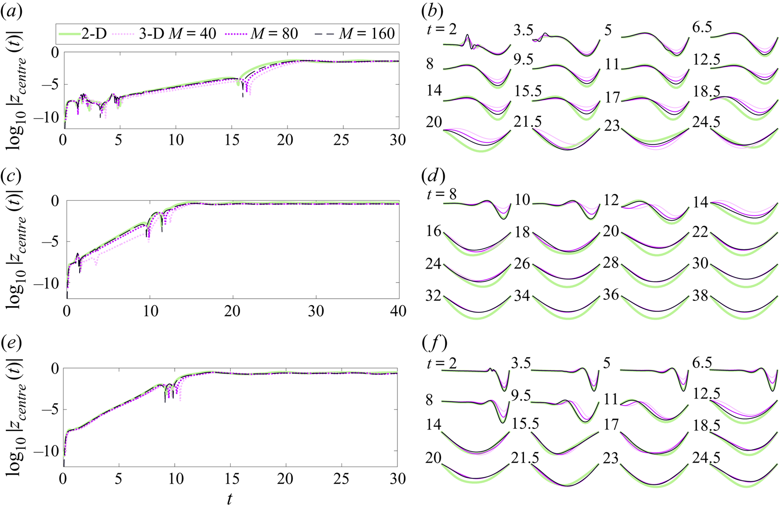
Figure 3. Comparisons of fixed–fixed (2-D) and FRFR (3-D) computations at three choices of  $(R_1,T_0,R_3)$: (a,b) $(10^{0},10^{-0.25},10^{3})$, (c,d) $(10^{-0.5},10^{-0.5},10^{1})$ and (e, f) $(10^{0.25},10^{-0.75},10^{1.5})$. Recall that $R_1$ is the dimensionless membrane mass, $T_0$ is the dimensionless pretension and $R_3$ is the dimensionless stretching rigidity. Panels (a,c,e) show plots of $\log _{10}|z_{{centre}}|$ vs time. Panels (b,d, f) show snapshots of membranes at equally spaced times (labelled at top left). The plots and snapshots are green for 2-D membranes and light pink ( $M = 40$), dark pink ( $M = 80$) or black ( $M = 160$) for 3-D membranes. Here, the aspect ratio $W/2L = 4$, $N=10$ and $\sigma =10^{-6}$ in (4.2).
To the right of each set of time plots, membrane snapshots are shown, equally spaced in time, for two dimensions (green lines) and three dimensions (with the same colours as in the time plots, for each  $M$), where the line shows the midspan profile. In all three examples, the membranes tend to a steady single-hump shape at large times, as shown for the 2-D case in Mavroyiakoumou & Alben (Reference Mavroyiakoumou and Alben2020). In figure 3 there is good qualitative agreement in all the membranes’ motions, and good quantitative agreement in most cases, particularly between $M=160$ (black lines) and two dimensions (green lines) in the small-amplitude (growth) regime. At later times, the 3-D snapshots tend to converge, while the 2-D snapshot is noticeably displaced from them, particularly in panel (d). The 3-D results apparently converge to slightly different states than the 2-D results. Some difference is inevitable due to the finite span in three dimensions and the corresponding difference in the flow and membrane dynamics.
Next we compare the 2-D fixed–free case with the 3-D FRRR case. Now the trailing edge is free, and a small transient perturbation is applied at the leading edge
 \begin{equation} z_{2\hbox{-}{\rm D}}({-}1,t)
= z_{3\hbox{-}{\rm D}}({-}1,\alpha_2,t) =
\sin\left(\sigma\left(\frac{t}{\eta}\right)^3\mathrm{e}^{-(t/\eta)^3}\right)
, \quad -\frac{W}{2L} \leq \alpha_2 \leq \frac{W}{2L}.
\end{equation}
\begin{equation} z_{2\hbox{-}{\rm D}}({-}1,t)
= z_{3\hbox{-}{\rm D}}({-}1,\alpha_2,t) =
\sin\left(\sigma\left(\frac{t}{\eta}\right)^3\mathrm{e}^{-(t/\eta)^3}\right)
, \quad -\frac{W}{2L} \leq \alpha_2 \leq \frac{W}{2L}.
\end{equation}
Figure 4 compares the membranes’ centre-point deflections and snapshots similarly to figure 3 but at three different choices of  $(R_1,T_0,R_3)$, given in the figure 4 caption. In the fixed–free case, oscillatory motions occur at large amplitude (Mavroyiakoumou & Alben Reference Mavroyiakoumou and Alben2020), and they tend to be periodic rather than chaotic at the $O(1)$ values of $R_1$ used in figure 4. Again, there is good qualitative agreement in all cases, and good quantitative agreement particularly in the linear growth regime. At large times in panels (a,b) and (e, f) the three 3-D cases are clustered together and are somewhat separate from the 2-D case. In panels (c,d) the $M = 160$ and 2-D case are relatively close, even at large times. Within each panel the graphs have somewhat different periods of oscillation at large amplitude, including some abrupt changes in the period, e.g. the 2-D graph near the final time in panels (e, f). However, if we compare the snapshots at qualitatively similar times, i.e. at nearby peaks and troughs of the $\log _{10}|z_{{centre}}(t)|$ plots, instead of at the same times, then we find better agreement. Comparisons of the 2-D case and the 3-D case with $M = 160$ at nearby peaks and troughs are shown below the time plots, and show better agreement than in the late-time comparisons on the right-hand side of the figure.

Figure 4. Comparisons of fixed–free (2-D) and FRRR (3-D) computations at three choices of  $(R_1,T_0,R_3)$: (a,b) $(10^0,10^{-1},10^2)$, (c,d) $(10^{-0.5},10^{-1},10^{2})$ and (e, f) $(10^{0.5},10^{-0.5},10^{2})$. Panels (a,c,e) show plots of $\log _{10}|z_{{centre}}|$ vs time. Panels (b,d, f) show snapshots of membranes at equally spaced times (labelled at top left). The plots and snapshots are green for 2-D membranes and light pink ( $M = 40$), dark pink ( $M = 80$) or black ( $M = 160$) for 3-D membranes. Here, the aspect ratio $W/2L = 4$, $N=10$ and $\sigma =10^{-6}$ in (4.3).
Finally, we compare the free–free 2-D case with 3-D RRRR cases. Now the membrane starts with a small non-zero slope
 \begin{equation} z_{2\hbox{-}{\rm D}}(\alpha_1,0) = z_{3\hbox{-}{\rm D}}(\alpha_1,\alpha_2,0) = \sigma \alpha_1 , \quad -\frac{W}{2L} \leq \alpha_2 \leq \frac{W}{2L}, \end{equation}
for  $\sigma =10^{-3}$. In figure 5 we again compare the membranes’ deflections and snapshots for three different $(R_1,T_0,R_3)$ combinations (in the figure caption) with $R_1 = O(1)$ that have qualitatively different dynamics. With all edges free, the membrane can move uniformly upward or downward yet keep the same shape, so there is a translational $z$ motion to consider along with the evolution of the membrane shape. Therefore, on the left-hand side we plot the membrane deflection vs time, defined here as $|\max (z)-\min (z)|$, with max and min taken over $\alpha _1$ (and $\alpha _2$ for three dimensions), and we also plot $z_{{centre}}(t)$, which shows the net translational motion. Panel (a) shows an oscillatory motion of $z_{{centre}}$, (c) shows a steady translation and (e) shows a combination of the two. As in the fixed–fixed and fixed–free cases, in each panel the agreement in the deflection $|\max (z)-\min (z)|$ is generally best at early times, and at later times there is a more noticeable difference, particularly between the 2-D and 3-D plots in panels (c,d) and (e, f). The snapshots at the right show that in many cases the shapes agree well but there is a translational shift, particularly at $t = 8$ in (b) (where the shift is small, $\approx 10^{-3}$) and at larger times in ( f). As in the fixed–free case, there are noticeable phase shifts among the motions at later times for the oscillatory case in panel (b).

Figure 5. Comparisons of free–free (2-D) and RRRR (3-D) computations at three choices of  $(R_1,T_0,R_3)$: (a,b) $(10^{-0.5},10^{-0.75},10^1)$, (c,d) $(10^{0.5},10^{-0.5},10^2)$ and (e, f) $(10^{-0.25},10^{-0.8},10^2)$. Panels (a,c,e) show plots of $\log _{10}|\max (z)-\min (z)|$ and $z_{{centre}}$ vs time. Panels (b,d, f) show snapshots of membranes at equally spaced times (labelled at top left). The plots and snapshots are green for 2-D membranes and light pink ( $M = 40$), dark pink ( $M = 80$) or black ( $M = 160$) for 3-D membranes. Here the aspect ratio $W/2L = 4$, $N=10$ and $\sigma =10^{-3}$ in (4.4).
In summary, the comparisons of 3-D motions at  $M$ = 40, 80 and 160 and the 2-D motion have shown good qualitative agreement in the types of dynamics – steady or oscillatory, with or without translation – and good quantitative agreement as well in the magnitudes of the deflections, the frequencies of oscillations and many detailed aspects of the dynamics.
Inviscid simulations of airfoils and flapping plates in two dimensions and three dimensions have shown that the largest computational errors tend to occur in flow quantities near the trailing edge (Katz & Plotkin Reference Katz and Plotkin2001; Alben Reference Alben2008a, Reference Alben2010; Hiroaki et al. Reference Hiroaki, Hayashi and Watanabe2021). The Kutta condition makes the flow velocity and pressure jump finite there, but their spatial derivatives across the edge are infinite there in general (Alben Reference Alben2010), and the numerical solution is sensitive to the mesh near the trailing edge (Alben Reference Alben2010; Hiroaki et al. Reference Hiroaki, Hayashi and Watanabe2021). For the present simulations, this sensitivity can be seen in the pressure jump distribution near the trailing edge. In figure 6 we plot the pressure jump vs streamwise location along the membrane midspan,  $y = 0$, for two different examples of FRRR membranes in the large-amplitude regime, at $R_1$, $T_0$ and $R_3$ given in the figure caption, and for various $M$ listed at the top. Both cases reach oscillatory large-amplitude states, shown by the centre deflection vs time in panels (a) and (d), respectively. In panels (b) and (e) we compare the midspan deflections that occur at $|z_{{centre}}|$ peaks near $t = 14.5$ and troughs near 12.6, respectively – the peaks and troughs that occur in the orange boxes of panels (a,d). For each $M$ the times of the peaks/troughs are slightly different due to phase shifts, as in the snapshot comparisons in figure 4(a,c,e). Panels (c, f) show the midspan pressure jump distributions at these times. The pressure jump distributions are more oscillatory and have larger deviations at these $M$ than the deflections (b,e), perhaps because in the membrane equation (2.16) $[p]$ is balanced by terms that include second spatial derivatives of deflection, so $z$ is smoother than $[p]$. We also find oscillations with similar spatial length scales in $\partial _{tt} z$ (not shown), perhaps indicating the effect of membrane inertia and added mass on $[p]$. The pressure jump distributions in (c, f) only approximately reach zero at the trailing edge, more closely for larger $M$, which also resemble the generic square-root behaviour there, as well as the generic inverse-square-root behaviours at the leading edge (Golberg Reference Golberg1990; Alben Reference Alben2009, Reference Alben2010). Although the deviations from $M = 40$ to 320 are significant, the overall form of the $[p]$ and $z$ distributions at $M$ = 40 are reasonable approximations to those at $M$ = 320.

Figure 6. Two examples of how the pressure distribution changes with increasing numbers of streamwise panels. Panels (a–c) show plots of  $\log _{10}|z_{{centre}}|$ vs time and $z(\alpha _1,0,t_p)$ and $[p](\alpha _1,0,t_p)$ vs $x(\alpha _1,0,t_p)$, respectively, for an FRRR membrane with $R_1=10^{-0.25}$, $T_0=10^{-0.75}$ and $R_3=10^1$ at times $t_p$ where $|z_{{centre}}(t)|$ has a peak that is closest to 14.5 (enclosed in the orange square), for each $M$. Panels (d–f) show the same quantities for an FRRR membrane with $R_1=10^{0}$, $T_0=10^{-0.75}$ and $R_3=10^1$, for the troughs in $|z_{{centre}}(t)|$ nearest to $t_p\approx 12.6$. The plots are black for $M=40$, blue for $M=80$, red for $M=160$ and green for $M=320$. Here, the aspect ratio $W/2L=4$, $N=10$ and $\sigma =10^{-4}$ in (4.3).
Now we briefly present a comparison of the dynamics in two and three dimensions using different numbers of panels across the span for three dimensions:  $N$ = 10, 20 and 40. Figure 7 shows comparisons of (a) fixed–fixed, (b) fixed–free and (c) free–free 2-D cases with the corresponding 3-D cases at $M$ = 40 and aspect ratio 4. The 3-D plots converge more rapidly here with increasing $N$ than with increasing $M$ in the previous figures, similarly to tables 1 and 2. In the remainder of this work we use $N=10$.

Figure 7. Comparisons of 2-D and 3-D membrane deflections at three boundary conditions and  $(R_1,T_0,R_3)$ values: (a) fixed–fixed vs FRFR at $(10^0,10^{-0.25},10^3)$; (b) fixed–free vs FRRR at $(10^0,10^{-1},10^2)$; and (c) free–free vs RRRR at $(10^{-0.25},10^{-0.8},10^2)$, where both $\log _{10}| \max (z)-\min (z)|$ and $z_{{centre}}$ are plotted, at left and right, respectively. The plots are green for 2-D membranes and light pink ( $N = 10$), dark pink ( $N = 20$) or black ( $N = 40$) for 3-D membranes. Here, 41 Chebyshev–Lobatto points are used in two dimensions and for the 3-D cases $W/2L = 4$, $M=40$ and $\sigma$ = $10^{-6}$, $10^{-6}$ and $10^{-3}$, respectively in (a–c).
We have compared the small- and large-amplitude dynamics in two and three dimensions at several  $(R_1,T_0,R_3)$ values, and shown the effect of varying the numbers of streamwise and spanwise panels in three dimensions, $M$ and $N$, at aspect ratio 4. Next, we compare the dynamics across a much larger set of $R_1$ and $T_0$ values, but restricted to the small-amplitude regime (where $R_3$ has a negligible effect). We also show the effect of increasing the 3-D membrane aspect ratio from 1 to 8, approaching the 2-D limit.
4.3. Comparison of stability boundaries and mode shapes in two and three dimensions
The small-amplitude membrane dynamics can be organized in terms of the stability boundary in  $R_1$– $T_0$ space. We again apply the small perturbations (4.2)–(4.4) to the FRFR, FRRR and RRRR membranes, across a grid of values in $R_1$– $T_0$ space. At each $R_1$ we find exponential decay in membrane deflections above a critical $T_0$ and exponential growth below this $T_0$ (followed by large-amplitude, nonlinear dynamics). The stability boundary is the curve of critical $T_0$ vs $R_1$, and is found by interpolating between neighbouring $T_0$ points with positive and negative growth rates.
In figure 8 we compare the stability boundaries in the 2-D fixed–fixed (a), fixed–free (b) and free–free (c) cases with the 3-D FRFR, FRRR and RRRR cases, respectively, with 3-D aspect ratios 1, 2, 4 and 8. Two stability boundaries are shown for the 2-D case. The orange lines, from Mavroyiakoumou & Alben (Reference Mavroyiakoumou and Alben2020), are calculated from the growth rates in time-stepping simulations starting from small perturbations, as in the 3-D cases here. The red lines, from Mavroyiakoumou & Alben (Reference Mavroyiakoumou and Alben2021b), are calculated by linearizing the 2-D equations and solving the nonlinear eigenvalue problem; the imaginary parts of the eigenvalues are the growth rates. The eigenvalue method was able to identify very small positive growth rates at  $R_1 \geq 10^2$, too small to be distinguishable from no growth or very slow decay in the time-stepping method. Here, the red line has a sharply upward slope (similar to Tiomkin & Raveh (Reference Tiomkin and Raveh2017)), unlike the orange line. The stability boundaries for the 3-D cases with aspect ratios 1, 2, 4 and 8 range from light blue to dark blue. In (a) and at large $R_1$ in (b,c) the boundaries tend towards the 2-D boundaries as aspect ratio increases. As in studies of 3-D flexible plates (Eloy, Souilliez & Schouveiler Reference Eloy, Souilliez and Schouveiler2007; Eloy et al. Reference Eloy, Lagrange, Souilliez and Schouveiler2008; Banerjee et al. Reference Banerjee, Connell and Yue2015), more bodies are unstable at high aspect ratio, i.e. the stability boundary moves up as the aspect ratio increases. In the region of instability for aspect ratio 8, we compare the aspect ratio 8 midspan snapshots at small amplitude (black lines) with the 2-D snapshots (green lines) over a range of $R_1$ and $T_0$. In (a), all the membranes lose stability by divergence without flutter, so the membranes’ deflections grow exponentially without change of shape. The snapshots show the eigenmode shapes, which become more fore–aft asymmetric as $T_0$ decreases, although at large amplitude the membranes tend to single-hump shapes that are nearly fore–aft symmetric as in figure 3. The agreement is uniformly very good between two and three dimensions in panel (a).

Figure 8. Comparisons of stability boundaries in two dimensions (orange from Mavroyiakoumou & Alben Reference Mavroyiakoumou and Alben2020; red from Mavroyiakoumou & Alben Reference Mavroyiakoumou and Alben2021b) and three dimensions with aspect ratios 1, 2, 4 and 8 (ranging from light blue to dark blue) for (a) fixed–fixed and FRFR, (b) fixed–free and FRRR and (c) free–free and RRRR cases. Below the stability boundary, 3-D midspan profiles with aspect ratio 8 (black) are compared with 2-D profiles (green) during the linear growth regime. Here,  $R_3=10^1$, $N=10$, $M=40$ (for FRFR and FRRR membranes) and $M=80$ (for RRRR membranes) for all aspect ratios.
Panel (b) shows the same comparison for the 2-D fixed–free and 3-D FRRR cases. The modes are somewhat underresolved for  $T_0 < 10^{-1}$ and the growth rates in two and three dimensions do not agree well, so we omit the membrane snapshots in this region of the parameter space. Even with a much finer mesh, the fastest growing 2-D modes are difficult to resolve in this region using an eigenvalue solver (Mavroyiakoumou & Alben Reference Mavroyiakoumou and Alben2021b). This underresolution may affect the apparent lack of convergence of the 3-D stability boundaries with increasing aspect ratio to the 2-D boundaries at small $R_1$. At moderate $R_1$ ( $\in [10^{-0.5},10^{0.5}]$), interestingly, the stability boundaries approximately coincide at all aspect ratios, while at larger $R_1$ the stability boundaries shift upward with increasing aspect ratio similarly to panel (a). Unlike in panel (a), here the snapshots oscillate and change shape in the small-amplitude growth regime. In panel (d) we show sets of six snapshots for the 2-D (green) and 3-D (black) cases during time intervals between two consecutive peaks or troughs in the graph of $z_{{centre}}(t)$. The snapshots are normalized to have uniform maximum deflections. The agreement between two and three dimensions is very good in all cases. The third snapshots in each sequence are overlaid in the instability region in panel (b). In (b,d) the values of $\log _{10} R_1$ and $\log _{10} T_0$ for each set of snapshots are the multiples of 0.5 and 0.25 respectively that intercept each set.
Panels (c,e) show the same comparison for the 2-D free–free and 3-D RRRR cases. The stability boundaries and resolution issues are similar to those in panel (b), but here adequate resolution is obtained down to smaller  $T_0$. At small $R_1$ values, the 3-D stability boundaries actually move away from the 2-D boundaries as the aspect ratio increases. This is due to special cases with very small but positive growth rates over a large range of $T_0$ at small $R_1$. Cases with aspect ratio 8 and growth rates < 0.04 are marked in panel (c) by grey boxes. Such cases only occur close to the stability boundary at large $R_1$, as expected, but occur over a large range of $T_0$ from the dark blue line to the orange (2-D) line at small $R_1$. Below the orange line, the 3-D growth rates abruptly become much larger, so setting aside the cases with very slow growth, we have better agreement in the stability boundary for two and three dimensions with aspect ratio 8. There is nothing obviously wrong with these slow-growth cases (such as very jagged shapes or non-physical motions); unlike most of the results in this section, they may be a case where the 3-D large-span dynamics is qualitatively different from the 2-D dynamics.
The agreement between the snapshots in two (green) and three dimensions (black) in panels (c,e) is generally very good, although not quite as good as in (b,d), particularly in some cases at  $T_0 = 10^{-1}$ and $10^{-1.25}$ that are clearly underresolved. In (c,e) higher resolution is used: $M = 80$ for RRRR and 81 Chebyshev–Lobatto points are used in two dimensions, vs 40 and 41 respectively in (a,b,d). In four cases at the upper right of (c,e) $|z_{{centre}}|$ grows without oscillating, similarly to a divergence instability, so the six snapshots are equally spaced over a large portion of the small-amplitude regime.
We have presented a broad range of evidence of good qualitative agreement between the 2-D and 3-D dynamics, even with fairly modest 3-D mesh sizes ( $M = 40$ and $N = 10$ in most cases) and other significant computational differences. In two dimensions we used a Chebyshev–Lobatto mesh, computed wake roll-up and used a Galerkin method for the kinematic equation and Kutta condition, with a non-flat body and wake in the kinematic condition. In three dimensions we used a uniform mesh, flat approximate vortex sheets on the body and wake and a collocation method for the kinematic condition. We now proceed to study and classify the dynamics of 3-D membranes with square aspect ratios at all 12 of the boundary conditions in figure 1.
5. Membrane dynamics across parameter space for 12 boundary conditions
We now broadly classify the membrane dynamics with respect to  $R_1$, $T_0$ and $R_3$ at all 12 combinations of fixed and free boundary conditions at the edges. In a few cases the large-amplitude dynamics does not seem to depend very strongly on aspect ratio, so we set it to 1 here, but it would be good to explore this parameter in future work.
To find where the membranes are unstable, we apply the perturbation (4.4) with  $\sigma =10^{-5}$ for all 12 boundary conditions at a large number of $R_1$ and $T_0$ values, and as before we find the critical $T_0$ at each $R_1$ by interpolation of growth rates.
Figure 9 shows the stability boundaries for the 12 boundary conditions, listed at right. Based on the locations of the boundaries and the qualitative features of membranes’ large-amplitude dynamics (presented later), the 12 boundary conditions naturally fall into four groups, listed at right in figure 9 and shown in figure 1, and determined by only the leading- and trailing-edge conditions. The conditions at these edges seem to determine the qualitative behaviours of the membranes’ dynamics more strongly than the side-edge conditions. However, the side edges can still have important effects, particularly for the large-amplitude results we will present.

Figure 9. Stability boundaries for the 12 boundary conditions, listed at right, and placed in four groups that depend on only the leading- and trailing-edge conditions, as in figure 1.
In the 2-D vs 3-D comparisons, we have already shown one stability boundary from three of the four groups: FRFR from group 1, FRRR from group 2 and RRRR from group 4. The other stability boundaries within these groups are similar – nearly flat in group 1, upward sloping in group 2 and either flat or upward sloping in group 4, although the flatness at small  $R_1$ for RRRR is affected by the slow-growth cases in figure 8(c). Perhaps due to these cases, there is more variability in the boundaries of group 4 at small $R_1$, while the boundaries are more uniform across groups 1 and 2. The data for group 3, with the leading edge free and trailing edge fixed, are completely new, and stand out from the other groups in two respects. The group 3 stability boundaries are orders of magnitude higher in $T_0$ than those of the other groups. There is also about an order-of-magnitude variation of the critical $T_0$ within group 3, higher (less stable) with more side edges free. At large $R_1$ it is difficult to distinguish slow growth and slow decay, particularly for RRFR, so the stability boundary is dashed to indicate this lack of certainty.
In the supplementary material, figure S1 marks  $(R_1, T_0)$ pairs where the small-amplitude instability corresponds to divergence or flutter with divergence, for each of the 12 boundary conditions. Divergence (without flutter) is most common for group 1 (fixed–fixed), while flutter with divergence is more common for the other three groups.
5.1. Large-amplitude scaling laws
We now study how key quantities – the typical magnitudes of deflections, and for unsteady cases, frequencies of oscillations – depend on  $R_1$, $T_0$ and $R_3$ in the large-amplitude regime. We set the perturbation magnitude $\sigma$ to 10 $^{-3}$ for groups 1, 2 and 4 and $10^{-2}$ for group 3, larger than the 10 $^{-5}$ value we used for the stability boundaries, to reach the large-amplitude regime faster. We also tested a few cases with different $\sigma$: $\pm 10^{-5}$ and several values ranging from $10^{-3}$ to $10^{-1}$. With $\sigma = -10^{-5}$ we obtained the mirror image of the large-amplitude steady state with $\sigma = 10^{-5}$. With different positive $\sigma$ and all other parameters the same, in most cases the same large-amplitude steady state was found (static or oscillatory). However, we did find one RFRF case where $\sigma = 10^{-3}, 10^{-2}$ and $0.03$ gave one steady shape and $\sigma = 0.06$ and 0.1 gave a different steady shape.
In our 2-D work (Mavroyiakoumou & Alben Reference Mavroyiakoumou and Alben2020, Reference Mavroyiakoumou and Alben2021b,Reference Mavroyiakoumou and Albena) we also studied the typical spatial wavenumbers of membrane deformations, but these are somewhat difficult to quantify precisely without higher spatial resolution, which is more feasible computationally in two dimensions. However, there is sometimes a correlation between wavenumbers and frequencies, which are computed here.
In figure 10 we show how the time-averaged deflection depends on  $R_3$ at several fixed values of $R_1$ (listed in the legends of panels (a,c,d)) and $T_0$ for all 12 boundary conditions. We define the time-averaged deflection of the membrane as the maximum membrane deflection minus the minimum deflection, averaged over time
 \begin{equation} \langle z_{{defl}}\rangle\equiv \frac{1}{t_2}\int_{t_1}^{t_1+t_2}\left(\max_{{-}1<\alpha_1,\alpha_2<1}z(\alpha_1,\alpha_2,t)-\min_{{-}1<\alpha_1,\alpha_2<1}z(\alpha_1,\alpha_2,t)\right)\,{\mathrm{d}} t, \end{equation}
where  $t_1$ and $t_2$ are sufficiently large that $\langle z_{{defl}}\rangle$ changes by less than $1\,\%$ with further increases in these values. As in the 2-D studies (Mavroyiakoumou & Alben Reference Mavroyiakoumou and Alben2020, Reference Mavroyiakoumou and Alben2021a), deflection scales as $1/\sqrt {R_3}$ at moderate and large $R_3$ in all 3-D cases. The scaling begins at larger $R_3$ for the third column, so the $R_3$ range there is a factor of $10^2$ higher than in the other columns. At $R_3 = 10^2$, the deflection magnitudes are generally much higher in column 3 than in the other columns. Selected $T_0$ values are shown in figure 10 but the same scaling holds at other $T_0$ values, two of which are shown in the Appendix. We briefly explain the $1/\sqrt {R_3}$ scaling similarly to Mavroyiakoumou & Alben (Reference Mavroyiakoumou and Alben2020). We expand terms in the $z$ component of the membrane equation (2.16) in the limit of small deflections, by inserting Taylor series for $z$ and its derivatives. $T_0$ and $R_3$ enter through the $\bar {e}$ and $K_s$ terms respectively. $T_0$ multiplies $(\partial ^2_{\alpha _1} + \partial ^2_{\alpha _2})z$ and $R_3$ multiplies a term that is cubic in derivatives of $z$. Using the kinematic and pressure jump equations, (2.19) and (2.20), we find that $\gamma _2$ is linear in $z$ and therefore so is $[p]$ and the $[p]$ term in (2.16). At steady state, the amplitude is set by a balance of the destabilizing $[p]$ term and the stabilizing $R_3$ term; the $T_0$ term is similar in magnitude to these terms near the stability boundary, and becomes insignificant at smaller $T_0$. Balancing $R_3 O(|z|^3)$ and the $O(|z|)$ pressure term, we have $|z| \sim R_3^{-1/2}$.

Figure 10. Time-averaged deflections of the membranes (defined by (5.1)) vs  $R_3$ for various $R_1$ (listed in the top panel of each column, i.e. panels (a,c,d), except (column 2) which uses the same values as panel (a)) and fixed $T_0$ for all 12 boundary conditions. Recall that $R_1$ is the dimensionless membrane mass, $T_0$ is the dimensionless pretension and $R_3$ is the dimensionless stretching rigidity. Panels (a,e,i), (b, f,j), (c,g,k) and (d,h,l) correspond to groups 1–4 in figures 1 and 9. The dotted black line in each panel indicates the scaling $R_3^{-1/2}$.
In the third column, smaller  $R_1$ values (listed in the top panel) are used compared with the other columns, because the third-column cases did not reach large amplitude within 350 time units at the larger $R_1$. In a few cases data are omitted because membranes were stable (FFRF with $R_1=10^{-0.5}$) or did not attain steady-state motions by $t$ = 350 (RRFF and RRFR with $R_1=10^{0.5}$).
The other main quantity we measure is the membrane’s frequency of oscillation. This is calculated as the reciprocal of the period of oscillation, the time between successive peaks in  $z_{{centre}}(t)$ near the end of the computation (typically $t = 350$). We plot the frequency data in figure 11, similarly to the amplitude data in the previous figure, but now vs $R_1$, the most important parameter for frequency, at various fixed values of $T_0$ and $R_3$ (listed in the titles and in the legends in the first two columns, respectively). Unlike the amplitude, the membranes’ shapes and frequencies do not vary much with $R_3$. In most cases with large $R_1$ ( $\in [10^1, 10^2]$) and some cases with moderate $R_1$ ( $\in [10^0, 10^1]$), the frequency approximately scales as $1/\sqrt {R_1}$, as in the large-amplitude 2-D studies Mavroyiakoumou & Alben (Reference Mavroyiakoumou and Alben2020, Reference Mavroyiakoumou and Alben2021a). The scaling can be explained in two or three dimensions by balancing the $R_1\partial _{tt}z$ term in the membrane equation with the other terms, which are independent of $R_1$. Assuming a period of oscillation $T$, we have $R_1\partial _{tt}z \sim R_1 z/T^2 \sim O(z)$ for the remaining terms (i.e. the $[p]$ term), so at large $R_1$ the frequency $= 1/T \sim 1/\sqrt {R_1}$.

Figure 11. Plots of mean frequency  $\log _{10}f$ vs mass density $\log _{10}R_1$ with various $R_3$ and fixed $T_0$ values for all 12 boundary conditions. Panels (a,e,i), (b, f,j), (c,g,k), (d,h,l) correspond to groups 1–4 in figures 1 and 9. The dotted black line in each panel indicates the scaling $R_1^{-1/2}$.
There is more variability in the frequency dependence on  $R_1$ than in the amplitude dependence on $R_3$, for a few main reasons. At large $R_1$, the oscillation period is longer, so longer times are needed to reach a steady state, and the estimates of period and frequency are based on smaller and perhaps noisier data sets. The oscillations are periodic in some cases but chaotic in others, and in the latter cases the frequency is only a rough estimate of the long-time average. Finally, the oscillatory motion may change qualitatively (e.g. the membrane shapes may change) as $R_1$ increases in the ranges considered here, which may cause deviations from the simple $1/\sqrt {R_1}$ scaling law.
At small  $R_1$ the frequency typically plateaus here (in the first and third columns). A different behaviour was seen in 2-D simulations of tethered membranes in Mavroyiakoumou & Alben (Reference Mavroyiakoumou and Alben2021a) which were similar to the 2-D free–free case. There, the frequencies scaled as $R_1^{-5/6}$ at small $R_1$ and the shapes had very sharp spatial features that required hundreds of points in the streamwise direction to resolve, much higher resolution than we use here in three dimensions. In the corresponding case here, the fourth column of figure 11, we have a limited set of data at small $R_1$ (at different $T_0$ than in the fourth column) that show increasing frequencies as $R_1$ decreases, but it is difficult to characterize the scaling behaviour. At small $R_1$ one might expect a plateau if the limit $R_1 \to 0$ is a regular perturbation problem, e.g. if the membrane shape does not change much in the limit $R_1 \to 0$, as seems to occur in the first and third columns. However, if the membrane becomes ever wavier as $R_1$ decreases, the frequency may also diverge, consistent with the 2-D tethered membrane data in Mavroyiakoumou & Alben (Reference Mavroyiakoumou and Alben2021a) and the closely related problem of a fixed–free flag with bending rigidity (Alben Reference Alben2022). The fourth and second columns, respectively, are similar to these cases.
The highest frequencies occur in the third column, and these are much higher than in the first column at the same  $R_1$. The third-column frequencies are only moderately higher than those in the second column at the $R_1$ where both are given, $10^{0.5}$.
One interesting difference with two dimensions that we will discuss further in the next section is that in three dimensions we find many cases of oscillatory membranes with leading and trailing edges fixed, corresponding to the frequencies in the first column. In two dimensions, all physically reasonable fixed–fixed cases assumed steady single-hump shapes. In panel (e) data are only presented at  $R_3 = 10^2$ and in panel (i) data are only presented at $R_3 = 10^0$, because the membranes did not oscillate at the other $R_3$ values across the full range of $R_1$ shown at these $T_0$.
5.2. Large-amplitude dynamics
We have presented basic scaling relationships for the amplitudes and frequencies of steady-state large-amplitude membrane motions. In this section we characterize the types of motions – e.g. a shape that is steady, or with periodic or chaotic oscillations – across all 12 boundary conditions. We consider in turn each of the four groups in figure 1, determined by the conditions at the leading and trailing edges. We use three values of the stretching rigidity parameter  $R_3$: $10^0$, $10^1$ and $10^2$. Somewhat below $10^0$, deflections become unrealistically large in some cases. At $R_3 = 10^2$, the motions generally approximate the large- $R_3$ asymptotic regime.
We consider values of  $T_0$ that are relatively close to the stability boundary, within 1–1.5 orders of magnitude of it. In general, as $T_0$ decreases, our algorithm requires more iterations for convergence at a given time step. At $T_0$ far below the stability boundary ( $\gtrsim 1.5$ orders of magnitude), the iterative method in our computational method tends to stagnate without converging at an early time step. In some cases, the stagnation occurs after a sharp angular feature appears in the membrane shape. Presumably larger $T_0$ inhibits the formation of such features. By contrast, our 2-D algorithm from Mavroyiakoumou & Alben (Reference Mavroyiakoumou and Alben2020, Reference Mavroyiakoumou and Alben2021a) was able to compute at arbitrarily small $T_0$, where the $T_0$ term became insignificant compared with the $R_3$ term in the total stretching force. There we found only modest changes in the dynamics as $T_0$ increased from zero to the stability boundary, so possibly the 3-D results here indicate what would happen at very small $T_0$, but we defer this question to future work.
In each case we consider a wide range of membrane mass  $R_1$, from small to large. Incidentally, we find that the iteration count increases at smaller $R_1$, but this does not prevent convergence, unlike at small $T_0$.
5.2.1. Leading and trailing edges fixed (FFFF, FRFF, FRFR)
We begin with membranes whose leading and trailing edges are fixed at zero deflection (group 1 in figures 1 and 9). Figure 12 shows typical motions and where they occur in parameter space. Each row of the top  $3\times 3$ array of panels corresponds to different side-edge conditions (FFFF, FRFF or FRFR), and each column to a different $R_3$ value ( $10^0$, $10^1$ or $10^2$). The different colours in each panel indicate where different types of motions occur in $R_1$– $T_0$ space, with representative examples below. Purple is used for steady single-hump shapes, green for small oscillations (periodic or not) about single-hump shapes, and yellow for up–down symmetric oscillations, usually periodic. Small black dots indicate periodic cases. Blue is used for cases that had slowly decaying oscillations at $t = 350$, and could approach the green or purple states at later times. Such cases occur at large $R_1$ and the oscillations tend to be less periodic than at smaller $R_1$. A few white regions in the upper corners of the FFFF panels indicate motions that were still in the exponential growth regime at $t = 350$, while cases in the white region in the FRFR panel at $R_3 = 10^0$ failed to converge at an early time. The three rows at the bottom of figure 12 show representative examples of the membrane motions in the purple, green and yellow regions. Just to the right of small rectangles with these colours, the motions are shown by sequences of 11 midspan snapshots (overlaid), and then further to the right, smaller sequences of four 3-D snapshots, arrayed horizontally. All these sequences are for FFFF cases, but single 3-D snapshots from the same type of motion with other side-edge conditions are shown at the far left in each row.

Figure 12. Typical membrane dynamics with fixed leading and trailing edges. The colour plots classify the different membrane dynamics across a grid of  $(R_1,T_0)$ values for three values of $R_3$ ( $10^0,10^1,10^2$) with black dots indicating periodic motions. Recall that $R_1$ is the dimensionless membrane mass, $T_0$ is the dimensionless pretension and $R_3$ is the dimensionless stretching rigidity. Representative examples of motions in the purple, green and yellow regions are shown in (d–f), identified by small coloured rectangles. To the right of the rectangles are overlaid sequences of 11 midspan snapshots in black, for FFFF boundary conditions. To the right of the midspan snapshots are a smaller representative sequence of four 3-D snapshots, from left to right with increasing time. To the left of the midspan snapshots are single 3-D snapshots representing similar cases with other side-edge conditions (FRFF and FRFR).
As noted previously, only steady single-hump shapes (purple) occur in two dimensions with fixed leading and trailing edges (Mavroyiakoumou & Alben Reference Mavroyiakoumou and Alben2020), whereas steady-state oscillations are surprisingly common in three dimensions, particularly with all four edges fixed. Here, up–down symmetric periodic motions (yellow) are much more common than with the other side-edge conditions, which typically have moderately small or no oscillations about a single-hump shape. The yellow motion includes a travelling wave of deflection that moves upstream, unlike in the 2-D fixed–free and free–free cases (Mavroyiakoumou & Alben Reference Mavroyiakoumou and Alben2020). Compared with the steady purple shape, the green motion has more variability not just in time but also in the spanwise direction, exemplified by the snapshot to the left of the small green rectangle in the second row from the bottom. In experiments, oscillatory cases with fixed leading and trailing edges have been reported mainly at non-zero angle of attack, where leading-edge vortex shedding seems particularly significant (Rojratsirikul, Wang & Gursul Reference Rojratsirikul, Wang and Gursul2010, figure 4). Fewer details have been given for unsteady motions at zero angle of attack in experiments (Galvao et al. Reference Galvao, Israeli, Song, Tian, Bishop, Swartz and Breuer2006).
5.2.2. Leading edge fixed and trailing edge free (FFRF, FRRF, FRRR)
The typical motions are qualitatively different in the second group (group 2 in figures 1 and 9), with the leading edge fixed and the trailing edge free. Hence, we classify the motions somewhat differently in figure 13, with colours denoting the number of times the midspan profile crosses  $z=0$ (not including the leading edge), time averaged. This classifies the spatial waviness of the profiles. Here, $R_3$ is fixed at $10^1$; at other $R_3$ the deflection amplitude varies but the numbers of zero crossings are almost unchanged. The numbers of zero crossings decrease almost monotonically as $R_1$ increases, and chaotic states (without black dots) with larger amplitudes and more up–down asymmetry become more common, similarly to the 2-D results in Mavroyiakoumou & Alben (Reference Mavroyiakoumou and Alben2020). In the white regions at the upper left of each panel, membranes are stable. In the white regions at the lower right, the computations did not converge when the membranes reached large amplitude but before they attained a steady-state motion, so results are not reported.

Figure 13. Typical membrane dynamics with fixed leading edges and free trailing edges. The colour plots in (a) show the time-averaged number of zero crossings of the membranes’ midspan profiles at various ( $R_1$, $T_0$) values for $R_3=10^1$. The black dots indicate periodic motions. Representative examples of motions at a sequence of $R_1$ values from $10^{-1}$ to $10^{1.5}$ are shown in (b–g). Overlaid sequences of 11 midspan snapshots are shown in black, for FRRF boundary conditions. To the right of the midspan snapshots are a smaller representative sequence of four 3-D snapshots, from left to right with increasing time. To the left of the midspan snapshots are single 3-D snapshots representing similar cases with other side-edge conditions (FFRF and FRRR).
Typical membrane motions are shown in the rows at the bottom, one for each  $R_1$ in a sequence from $10^{-1}$ to $10^{1.5}$. Here, the motions resemble different modes of a flapping flag (Connell & Yue Reference Connell and Yue2007; Alben Reference Alben2008b, Reference Alben2022), with travelling waves that pass downstream, unlike for group 1. Another difference here is that the side-edge conditions do not change the type of motion. As in Mavroyiakoumou & Alben (Reference Mavroyiakoumou and Alben2020), at small $R_1$ the deflection envelope has small amplitude near the trailing edge. At large $R_1$ (e.g. $10^{1.5}$) the travelling waves become more like standing waves, with fixed nodes and antinodes.
5.2.3. Leading edge free and trailing edge fixed (RFFF, RRFF, RRFR)
Next, we consider membranes whose leading edge is free and trailing edge is fixed (group 3 in figures 1 and 9). We showed in figure 9 that here the critical pretensions for instability are much larger than in the other cases. The space of motions is qualitatively different than for groups 1 and 2. In figure 14, we identify just three types of motions, with approximately periodic, up–down symmetric oscillations in most cases, characterized by three typical midspan profiles shown in the bottom three rows: a low-mode shape with at most a single interior  $z$ extremum (light purple), a higher-mode shape with one or two interior $z$ extrema (yellow) and a low-mode shape with a multi-valued $z$ profile near the trailing edge at certain times (dark purple). This last motion is more common at smaller $R_1$ and does not appear with both side edges fixed or at the largest $R_3$ (right column), where the first motion dominates. White regions are again cases in which the computations did not converge when the membranes reached large amplitude but before they attained a steady-state motion. Another special feature of group 3 is that the small-amplitude growth rates are generally much less than in the other groups, so data are omitted for $R_1 > 10^0$ because the amplitudes were growing and had not yet reached a steady state at $t = 350$. In some cases at $R_1 = 10^{1.5}$ and $10^2$ (not shown) the amplitude neither grows nor decays noticeably after the initial perturbations, as also occurred in some 2-D cases at large $R_1$ (Mavroyiakoumou & Alben Reference Mavroyiakoumou and Alben2020).

Figure 14. Typical membrane dynamics with free leading edges and fixed trailing edges. The colour plots classify the different membrane dynamics across a grid of  $(R_1,T_0)$ values for three values of $R_3$ ( $10^0,10^1,10^2$) with black dots indicating periodic motions. Representative examples of motions in the light purple, yellow and dark purple regions are shown in (d–f), identified by small coloured rectangles. To the right of the rectangles are overlaid sequences of 11 midspan snapshots in black, for RFFF boundary conditions (d,e) and RRFF boundary conditions ( f). To the right of the midspan snapshots are a smaller representative sequence of four 3-D snapshots, from left to right with increasing time. To the left of the midspan snapshots are single 3-D snapshots representing similar cases with other side-edge conditions (RRFR and RRFF).
The motions of group 3 seem more likely to violate the physical assumptions of the model than the other groups. The oscillation amplitude is highest at the leading edge, so leading-edge vortex shedding is probably important unless the oscillation amplitudes are very small (i.e. at  $R_3 = 10^3$ and $10^4$, where the motions are similar to those in the $R_3 = 10^2$ column, light purple generally). Vortex shedding would probably occur in multiple locations upstream of the trailing edge for the dark purple motions, due to large deflection amplitudes and slopes.
5.2.4. Leading and trailing edges free (RFRF, RRRF, RRRR)
Group 4 consists of membranes with the leading and trailing edges free (figures 1 and 9). With fewer of the edges fixed, we find a wider variety of dynamics. In figure 15 we use seven categories to classify the motions, with representative examples in the seven rows at the bottom, each labelled using a small rectangle with a certain colour and symbol that is repeated at data points in this category in the  $3\times 3$ array of colour plots above. The first three rows represent categories of steady shapes with one, two or three internal inflection points, respectively. The fourth row represents a category of motions with small oscillations about one of the steady shapes. To identify these cases, we decompose the midspan deflection $z(\alpha _1,0,t)$ as the sum of its time average and the remainder, the unsteady part. Motions are in the fourth category if the maximum minus the minimum of the unsteady deflection is non-zero but much less than the maximum minus the minimum of the time-averaged deflection. The fifth row represents unsteady motions whose unsteady part is comparable to or larger than the steady part (in the same sense as for the fourth category). The sixth row is for a special type of unsteady motion with all edges free (RRRR) that is time periodic. These motions have translational and deformational dynamics with $O(1)$ frequencies, and their translational motions are more precisely time periodic than those at large $R_1$. The seventh row is for another special type of unsteady RRRR motion that has both large spanwise and large chordwise curvatures.

Figure 15. Typical membrane dynamics with free leading and trailing edges. The colour plots classify the different membrane dynamics across a grid of  $(R_1,T_0)$ values for three values of $R_3$ ( $10^0,10^1,10^2$) with black dots indicating periodic motions. Representative examples of motions in all the coloured regions are shown in (d–j), identified by small coloured rectangles with symbols. To the right of the rectangles are overlaid sequences of 11 midspan snapshots in black, for RFRF (d, f,g,h), RRRF (e) and RRRR boundary conditions (i,j). To the right of the midspan snapshots are a smaller representative sequence of four 3-D snapshots, from left to right with increasing time. To the left of the midspan snapshots are single 3-D snapshots representing similar cases with other side-edge conditions (RRRF and RRRR).
The sixth and seventh categories occur only for the RRRR case, which seems to have a wider variety of motions because it is free to translate in  $z$. As in the 2-D case (Mavroyiakoumou & Alben Reference Mavroyiakoumou and Alben2020), the translational motion is distinct from but coupled to the shape deformation dynamics, and the combination of the two results in more types of dynamics. Other categories of motions that occur only with certain edge conditions are the second and third, the steady states with two or three interior inflection points, respectively. The second occurs for RRRF and RRRR and the third for RFRF, both mainly at small $R_1$. The fourth category, small oscillations about a steady shape, occurs only with one or both side edges fixed (RFRF and RRRF). The first category, a steady shape with a single inflection point, occurs with all side edge conditions, but in the RRRR case it translates either up or down in $z$ at almost constant speed, with occasional reversals in direction (as in Mavroyiakoumou & Alben Reference Mavroyiakoumou and Alben2020, figure 20). The fifth category, of general unsteady motions, occurs with all side-edge conditions at large $R_1$. Here, motions tend to be more asymmetrical and irregular and have larger oscillation amplitudes. The large body mass may allow the body to maintain its momentum against resisting fluid forces for longer times.
6. Conclusions
We have developed a model and numerical method to compute the small- and large-amplitude dynamics of thin membranes in 3-D inviscid flows. We provided numerical evidence that indicates convergence of our method with respect to spatial grid refinement. The 3-D solutions agree remarkably well with those computed in 2-D flows with different discretization techniques, particularly when the aspect ratio in three dimensions is large.
With fixed or free boundary conditions at each of the four edges, we have 16 combinations of boundary conditions for rectangular membranes, reduced to 12 when symmetric cases are accounted for. We computed the dynamics in all 12 cases with various values of the three key physical parameters: membrane mass ( $R_1$), pretension ( $T_0$) and stretching rigidity ( $R_3$). The 12 cases fit naturally into four groups that are determined by the leading- and trailing-edge boundary conditions. Within each group there are strong similarities in the shapes and locations of the stability boundaries, the typical magnitudes of membranes’ deflections and their oscillation frequencies in unsteady cases, and the typical shapes of the membranes at the midspan location. The side-edge boundary conditions can cause small or large qualitative differences in the dynamics within each group. The differences are relatively small for the fixed–free case (group 2); the midspan shape is almost unchanged at a free side edge or gradually scaled to flat at a fixed side edge. The differences are larger for the fixed–fixed and free–fixed cases (groups 1 and 3); changes in side-edge conditions lead to the appearance or disappearance of certain types of oscillation modes. In group 4 (free–free) the side edges have an even larger effect, for example by allowing or preventing translational motions that lead to a wider variety of dynamics.
As in two dimensions, the deflection magnitudes scale as  $R_3^{-1/2}$ and the oscillation frequencies scale as $R_1^{-1/2}$ at large values of $R_3$ and $R_1$ respectively. The stability boundaries and dynamics in groups 1, 2 and 4 have many resemblances to the 2-D cases with same leading- and trailing-edge conditions studied in Mavroyiakoumou & Alben (Reference Mavroyiakoumou and Alben2020). The fixed–free case in three dimensions is very similar to the 2-D case in terms of increasing waviness with decreasing $R_1$, a more limited effect of $T_0$ on the shapes and $R_3$ mainly setting the amplitudes of oscillation but not the shapes. The free–free case in three dimensions has some of the same types of states as in two dimensions: periodic oscillatory states and vertical translational states that may be nearly steady with a non-zero mean slope, or undergo periodic or chaotic oscillations.
However, there are important qualitative differences in three dimensions. Unlike the 2-D fixed–fixed case where all membranes converge to steady single-hump shapes, the 3-D version (group 1) has cases with small and large unsteady oscillations, particularly when both side edges are fixed. The 3-D results contradicted our intuition from the 2-D study that more fixed edges lead to fewer unsteady states. The 3-D free–free case (group 4) has complicated spanwise curvature distributions, particularly with one or both side edges free. There are more types of motions here than in the 2-D free–free case. We did not study the 2-D analogue of group 3, free–fixed, but the variations with side-edge conditions here show that 3-D effects can be significant. Taken together these results validate the use of 2-D models for a good qualitative understanding of membrane motions and scaling with parameters, but also show that certain important phenomena can only be seen with the 3-D model.
Future work could investigate several topics, for example: the effect of aspect ratio; a non-zero Poisson ratio; including non-flat vortex sheets in the kinematic condition and computing wake roll-up (e.g. using a tree code Lindsay & Krasny Reference Lindsay and Krasny2001) and consequences for the membrane dynamics, especially at large mass density ratio and small stretching rigidity (Mavroyiakoumou & Alben Reference Mavroyiakoumou and Alben2020, figures 17 and 23); the types of motions at smaller  $T_0$, which would require altering the algorithm to be able to compute steady-state motions in this regime; mixed fixed and free boundary conditions on a single edge; and different membrane shapes.

Figure 16. Time-averaged deflections of FRFR and FRFF membranes (defined by (5.1)) vs  $R_3$ for various $R_1$ and fixed $T_0$ ( $10^{-0.25}$ and $10^{-0.75}$). The dotted black line indicates the scaling $R_3^{-1/2}$.
Supplementary material and movies
Supplementary material and movies are available at https://doi.org/10.1017/jfm.2022.957.
Funding
We acknowledge support from a Rackham Predoctoral Fellowship Award (University of Michigan) and the NSF Mathematical Biology program under award number DMS-1811889.
Declaration of interests
The authors report no conflict of interest.
Appendix. Membrane deflections vs stretching rigidity at different pretension values
For two of the 12 boundary conditions (FRFF and FRFR) we plot in figure 16 the average membrane deflection at  $T_0=10^{-0.25}$ and $10^{-0.75}$, instead of $10^{-0.5}$ in figure 10, and see that the deflection values increase at smaller $T_0$ (similarly to Mavroyiakoumou & Alben Reference Mavroyiakoumou and Alben2020; Tiomkin & Jaworski Reference Tiomkin and Jaworski2022) but the same $1/\sqrt {R_3}$ scaling holds in all cases.


 Open access