


1. Introduction
The transport of fluid associated with the progression of contraction/expansion waves along a tube plays a fundamental role in many physiological phenomena and technological applications (Jaffrin & Shapiro Reference Jaffrin and Shapiro1971). In many situations, the Reynolds number is small and the wavelength is large compared with the tube transverse dimension, so that the motion can be described in the lubrication approximation. The seminal analysis of Shapiro, Jaffrin & Weinberg (Reference Shapiro, Jaffrin and Weinberg1969), corresponding to peristaltic motion driven by a train of sinusoidal waves travelling along an infinitely long tube of circular section, has been extended to account for effects of different cross-sectional shapes (Rath Reference Rath1982) and finite tube lengths (Li & Brasseur Reference Li and Brasseur1993), for example.
Peristaltic pumping driven by arterial pulsations due to the heartbeat has been reasoned to play a role in the transport of cerebrospinal fluid (CSF) along the perivascular spaces that surround cerebral arteries (Rennels et al. Reference Rennels, Gregory, Blaumanis, Fujimoto and Grady1985; Stoodley et al. Reference Stoodley, Brown, Brown and Jones1997; Hadaczek et al. Reference Hadaczek, Yamashita, Mirek, Tamas, Bohn, Noble, Park and Bankiewicz2006). The recent in vivo particle image velocimetry (PIV) measurements in mice of Mestre et al. (Reference Mestre, Tithof, Du, Song, Peng, Sweeney, Olveda, Thomas, Nedergaard and Kelley2018) have demonstrated that the resulting pulsatile motion of the CSF exhibits a net flow rate in the direction of the arterial blood flow – see also Raghunandan et al. (Reference Raghunandan, Ladrón-de-Guevara, Tithof, Mestre, Du, Nedergaard, Thomas and Kelley2021) for more recent experiments. The experiments also revealed that the periarterial space is a mostly unobstructed non-axisymmetric annular canal whose width is comparable to the arterial radius (Min Rivas et al. Reference Min Rivas, Liu, Martell, Du, Mestre, Nedergaard, Tithof, Thomas and Kelley2020). As reasoned by Thomas (Reference Thomas2019), because of the strong asymmetry of the cross-section, the associated flow characteristics and resulting pumping rate can be expected to differ significantly from those predicted for an axisymmetric annulus (Bilston et al. Reference Bilston, Fletcher, Brodbelt and Stoodley2003; Wang & Olbricht Reference Wang and Olbricht2011). The effects of asymmetry have been recently addressed using an inner circle (representing the artery) and an outer eccentric ellipse as an approximate model for the cross-sectional shape of the periarterial space. Attention has been given to the associated hydraulic resistance, which was evaluated by Tithof et al. (Reference Tithof, Kelley, Mestre, Nedergaard and Thomas2019), and to the periodic flow induced by a small-amplitude sinusoidal wave, which was described by Carr et al. (Reference Carr, Thomas, Liu and Shang2021) by integrating numerically the full Navier–Stokes equations over five cycles in a tube of length equal to two wavelengths. The latter analysis numerically explored the dependence of the pumping rate on the cross-sectional shape and pointed out the inherent three-dimensionality of the flow, arising in the absence of axial symmetry. These features of the solution are further investigated here by means of analytical methods that exploit simplifications arising for low-Reynolds-number slender flows. Despite the numerous simplifying approximations introduced in the description, the results have potential applicability in connection with the flow in the cerebral perivascular system, as discussed at the end of the paper.
As in the previous numerical simulations of Carr et al. (Reference Carr, Thomas, Liu and Shang2021), the present work considers peristaltic flow in a non-axisymmetric annular canal. Cylindrical coordinates  $(x',r',\theta )$ and corresponding velocity components $(u',v',w')$ are to be used in the analysis. As indicated in figure 1, the canal is bounded externally by a fixed cylinder of radius $r'_e(\theta )$, while the inner surface, representing the arterial wall supporting a travelling peristaltic wave, has a circular cross-section of radius $r'_a$, comparable in magnitude to the outer radius $r'_e$, given by
 \begin{equation} r'_a=r'_o [1+ \varepsilon \mathcal{T} (\kappa x'-\omega t')], \end{equation}
where  $t'$ is the time, and $\kappa$ and $\omega$ are the wavenumber and angular frequency, with $2 {\rm \pi}/\kappa$ representing the wavelength, assumed to be much longer than the characteristic canal transverse dimension (i.e. $\kappa r'_o \ll 1$). The wave is described by the general $2{\rm \pi}$-periodic function $\mathcal {T}(\xi )$ of the characteristic coordinate $\xi =\kappa x'-\omega t'$. This wavefunction satisfies $\int _0^{2 {\rm \pi}} \mathcal {T} \,\textrm {d}\xi =0$, so that $r'_o$ is the time-averaged radius. In periarterial flow, the specific shape of $\mathcal {T}(\xi )$, schematically represented in figure 1, is related to the cardiac pulsation, as revealed by in vivo temporal measurements of arterial diameters in the mouse brain (Mestre et al. Reference Mestre, Tithof, Du, Song, Peng, Sweeney, Olveda, Thomas, Nedergaard and Kelley2018), which also showed the relative wave amplitude $\varepsilon$ to be small, on the order of $\varepsilon \sim 0.02$.

Figure 1. The model problem considered, including the coordinate system and a schematic showing the typical arterial-wall wave shape.
2. The infinitely long tube
We begin by considering the case of an infinitely long tube undergoing peristaltic motion, for which the  $2{\rm \pi}$-periodic variations in the rescaled coordinates $t=\omega t'$ and $x=\kappa x'$ can be described in terms of the single characteristic coordinate $\xi =\kappa x'-\omega t'$. As discussed by Shapiro et al. (Reference Shapiro, Jaffrin and Weinberg1969), most of the results, including the associated volume flow rate $Q'(\xi )$, are in general applicable to tubes whose length $L$ is a multiple of the wavelength (i.e. $L=2 {\rm \pi}j /\kappa$, with $j=1,2,3,\ldots$).
The fluid in the annular canal has density  $\rho$ and viscosity $\mu$. To focus more directly on the conditions of interest for periarterial CSF flow, it is assumed that the characteristic viscous time $r_o^{\prime 2}/(\mu /\rho )$ satisfies $r_o^{\prime 2}/(\mu /\rho ) \ll \omega ^{-1}$, so that the motion is quasi-steady and with negligibly small inertia. The resulting Stokes equations further simplify as a result of the slenderness condition $r'_o \ll \kappa ^{-1}$, in that, with errors of order $(\kappa r'_o)^2$, longitudinal derivatives can be neglected when computing the viscous stresses. At the same level of approximation, the transverse variations of the pressure, which are a factor $(\kappa r'_o)^2$ smaller than the corresponding longitudinal variations, can be discarded when computing the axial flow.
The dimensionless formulation employs the coordinates  $\xi =\kappa x'-\omega t'$ and $r=r'/r'_o$, along with the order-unity velocity components $u=u'/(\varepsilon \omega /\kappa )$, $v=v'/(\varepsilon \omega r'_o)$ and $w=w'/(\varepsilon \omega r'_o)$, and corresponding flow rate $Q=Q'/(\varepsilon r_o^{\prime 2} \omega /\kappa )$. The accompanying spatial pressure variations $p'$ are expressed in the form
 \begin{equation} \frac{p'}{\mu \varepsilon \omega/(\kappa r'_o)^2}=p(\xi)+(\kappa r'_o)^2 \tilde{p}, \end{equation}
where the function  $\tilde {p}(\xi ,r, \theta )$ is introduced to measure the small pressure variations, of order $(\kappa r'_o)^2 \ll 1$, found across the section of the canal, which enter in the description of the transverse motion. In the lubrication approximation adopted here, the problem reduces to the integration of
 $$\begin{gather} -\frac{\textrm{d} p}{\textrm{d} \xi}+\frac{1}{r} \frac{\partial}{\partial r} \left(r \frac{\partial u}{\partial r} \right)+\frac{1}{r^2} \frac{\partial^2 u}{\partial \theta^2}=0, \end{gather}$$
 $$\begin{gather}-\frac{\partial \tilde{p}}{\partial r}+\frac{\partial}{\partial r} \left[\frac{1}{r} \frac{\partial}{\partial r} (r v) \right]+\frac{1}{r^2} \frac{\partial^2 v}{\partial \theta^2}-\frac{2}{r^2} \frac{\partial w}{\partial \theta} =0, \end{gather}$$
 $$\begin{gather}-\frac{1}{r} \frac{\partial \tilde{p}}{\partial \theta}+\frac{\partial}{\partial r} \left[\frac{1}{r} \frac{\partial}{\partial r} (r w) \right]+\frac{1}{r^2} \frac{\partial^2 w}{\partial \theta^2}+\frac{2}{r^2} \frac{\partial v}{\partial \theta} =0, \end{gather}$$
 $$\begin{gather}\frac{\partial}{\partial \xi} (r u)+\frac{\partial}{\partial r} (r v)+\frac{\partial w}{\partial \theta}=0, \end{gather}$$
with boundary conditions
 \begin{equation} \left.\begin{array}{c@{}} u=v+\dot{\mathcal{T}}(\xi)=w=0 \quad \textrm{at} \ r=a=1+\varepsilon \mathcal{T}(\xi), \\ u=v=w=0 \quad \textrm{at} \ r=r_e(\theta), \end{array}\right\} \end{equation}
where  $\dot {\mathcal {T}}=\textrm {d} \mathcal {T}/\textrm {d} \xi$, $a=r'_a/r'_o$ and $r_e(\theta )=r'_e/r'_o$.
3. The axial velocity
Following standard practice (White Reference White2006), the axial velocity can be expressed in the compact form  $u=-(\textrm {d} p/\textrm {d} \xi ) U$, where the function $U(r,\theta ;a)$ satisfies the Poisson problem
 \begin{equation} \frac{1}{r} \frac{\partial}{\partial r} \left(r \frac{\partial U}{\partial r} \right)+\frac{1}{r^2} \frac{\partial^2 U}{\partial \theta^2}={-}1, \quad U=0 \quad \textrm{at} \left\{\begin{array}{@{}l} r=a, \\ r=r_e(\theta),. \end{array} \right. \end{equation}
The accompanying volume flow rate becomes
 \begin{equation} Q=\int_0^{2{\rm \pi} } \left(\int_a^{r_e(\theta)} r u \, \textrm{d}r \right)\, \textrm{d} \theta={-}\frac{\textrm{d} p}{\textrm{d} \xi} \frac{1}{\mathcal{R}}, \end{equation}
in terms of the dimensionless hydraulic resistance
 \begin{equation} \mathcal{R}=\left[\int_0^{2{\rm \pi} } \left(\int_a^{r_e(\theta)} r U \, \textrm{d}r \right)\, \textrm{d} \theta \right]^{{-}1}. \end{equation}
 Simple solutions to (3.1) are available when the tube is a concentric circular annulus of outer radius  $r_e=b$ (White Reference White2006) and also for thin annular tubes of general shape satisfying $r_e-a \ll 1$, when the solution can be approximated by the expressions
 \begin{equation} U=(r-a)(r_e-r)/2 \quad \textrm{and} \quad \mathcal{R}^{{-}1}=(a/12) \int_0^{2{\rm \pi} } (r_e-a)^3\, \textrm{d}\theta. \end{equation}
 Numerical integration is in general needed to solve (3.1) for non-axisymmetric tubes with  $r_e-a \sim 1$, with results relevant to the periarterial cross-section computed by Tithof et al. (Reference Tithof, Kelley, Mestre, Nedergaard and Thomas2019). As in Carr et al. (Reference Carr, Thomas, Liu and Shang2021), illustrative results will be given below for two different outer boundaries $r_e(\theta )$, depicted at the top of figure 2, namely, a coaxial elliptical cylinder with semi-axis lengths $b r'_o$ and $c r'_o$, a configuration investigated by Shivakumar (Reference Shivakumar1973), and a circular cylinder of radius $b r'_o$ whose centre is displaced a distance $c r'_o$ from that of the inner circular cylinder, a configuration first studied by Piercy, Hooper & Winny (Reference Piercy, Hooper and Winny1933). In the latter case, the approximate expression
 \begin{equation} \mathcal{R}^{{-}1}=\frac{{\rm \pi} }{8} \left[1+\frac{3}{2} \left(\frac{c}{b-a}\right)^2\right]\left[b^4-a^4 -\frac{(b^2-a^2)^2}{\ln(b/a)}\right] \end{equation}
yields very accurate results provided that  $b$ is not too large (White Reference White2006).

Figure 2. (a,b) The two different outer boundaries (see text). (c–f) The values of  $\mathcal {R}_o$ and $\varDelta$ obtained from (3.7a,b) by numerical integration of (3.1) and (3.3) when the section of the outer cylindrical surface is an eccentric circle (c,e) and a concentric ellipse (d,f). The triangles denote approximate results evaluated with (3.8) and (3.9). (g,h) Comparison of the predicted value of the mean flow rate $\langle Q \rangle ={\rm \pi} \varepsilon \varDelta$ (solid lines) with the numerical results of Carr et al. (Reference Carr, Thomas, Liu and Shang2021) (crosses).
The function  $U$ and associated hydraulic resistance $\mathcal {R}$ depend on the characteristic coordinate $\xi$ through the inner radius $a=1+\varepsilon \mathcal {T}(\xi )$. The dependence is weak for cases with $\varepsilon \ll 1$, to be investigated below, for which expanding $\mathcal {R}$ in a Taylor series leads to
 \begin{equation} \mathcal{R}=\mathcal{R}_o [1+\varDelta \varepsilon \mathcal{T}(\xi)] + O(\varepsilon^2), \end{equation}
where
 \begin{equation} \mathcal{R}_o=\mathcal{R}|_{a=1} \quad \textrm{and} \quad \varDelta=\left. \frac{\textrm{d} \mathcal{R}/\textrm{d} a}{\mathcal{R}} \right|_{a=1}, \end{equation}
both evaluated at  $a=1$, are, respectively, the hydraulic resistance of the tube with constant inner radius $r'_a=r'_o$ and the relative variation of the hydraulic resistance in response to changes of the inner radius. Selected values of $\mathcal {R}_o$ and $\varDelta$, determined numerically with use of (3.1) and (3.3), are shown in figure 2 for the eccentric and elliptical annuli. For the former, figure 2 also shows predictions obtained using the simple approximate formulae
 \begin{equation} \mathcal{R}_o^{{-}1}=\frac{{\rm \pi} }{8} \left[1+\frac{3}{2} \left(\frac{c}{b-1}\right)^2\right] \left[b^4-1 -\frac{(b^2-1)^2}{\ln(b)}\right] \end{equation}
and
 \begin{equation} \varDelta=\frac{\displaystyle \left[1+\frac{3}{2} \left(\frac{c}{b-1}\right)^2\right] \left[4+\frac{b^2-1}{\ln b}\left(\frac{b^2-1}{\ln b}-4\right)\right]-\frac{3c^2}{(b-1)^3}}{\displaystyle \left[1+\frac{3}{2} \left(\frac{c}{b-1}\right)^2\right] \left[b^4-1 -\frac{(b^2-1)^2}{\ln(b)}\right]} \end{equation}
stemming from (3.5).
4. The pumping rate
The determination of the axial pressure gradient  $\textrm {d} p/\textrm {d} \xi$, which enters as a factor in $u=-(\textrm {d} p/\textrm {d} \xi ) U$, begins by integrating (2.5) across the tube section with the boundary conditions (2.6) to give
 \begin{equation}
\frac{\textrm{d}}{\textrm{d} \xi}
\left(-\frac{1}{\mathcal{R}} \frac{\textrm{d} p}{\textrm{d}
\xi} \right)+2 {\rm \pi}(1+\varepsilon
\mathcal{T}) \dot{\mathcal{T}}=0,
\end{equation}
\begin{equation}
\frac{\textrm{d}}{\textrm{d} \xi}
\left(-\frac{1}{\mathcal{R}} \frac{\textrm{d} p}{\textrm{d}
\xi} \right)+2 {\rm \pi}(1+\varepsilon
\mathcal{T}) \dot{\mathcal{T}}=0,
\end{equation}
upon substitution of (3.2) and  $a=1+\varepsilon \mathcal {T}(\xi )$. Integrating the above equation once gives
 \begin{equation} Q(\xi)={-}\frac{1}{\mathcal{R}} \frac{\textrm{d} p}{\textrm{d} \xi}=C_\lambda-2 {\rm \pi}(\mathcal{T} +\varepsilon \mathcal{T}^2/2), \end{equation}
involving the unknown integration constant  $C_\lambda$. Since $\int _0^{2 {\rm \pi}} \mathcal {T} \,\textrm {d} \xi =0$, taking the average of the above equation over a cycle provides
 \begin{equation} \langle Q \rangle=C_\lambda- {\rm \pi}\varepsilon \langle \mathcal{T}^2 \rangle \end{equation}
for the time-averaged pumping rate at any location. To facilitate the notation, averages of  $2{\rm \pi}$-periodic functions of a single independent variable are denoted throughout the paper by $\langle \cdot \rangle = \int _0^{2{\rm \pi} } (\cdot )\, \textrm {d} y/(2 {\rm \pi})$, where $y$ is a generic dummy integration variable, i.e. $y=\xi$ in (4.3).
The value of the constant  $C_\lambda$ in (4.3) can be obtained by multiplying (4.2) by $\mathcal {R}$ and integrating the resulting equation between $\xi =0$ and $\xi =2{\rm \pi}$ to give
 \begin{equation} C_\lambda=\frac{2 {\rm \pi}\langle \mathcal{T} \mathcal{R} \rangle+{\rm \pi} \varepsilon \langle \mathcal{T}^2 \mathcal{R} \rangle-\delta p_\lambda/(2{\rm \pi} )}{\langle \mathcal{R} \rangle}. \end{equation}
For generality, following the work of Shapiro et al. (Reference Shapiro, Jaffrin and Weinberg1969), in writing (4.4) we have assumed that the periodic streamwise pressure gradient  $\textrm {d}p/\textrm {d} \xi$ may have a steady component, associated with a pressure rise $\delta p_\lambda$ per wavelength.
The above results, which are valid for  $\varepsilon \sim 1$, can be simplified in the small-amplitude limit $\varepsilon \ll 1$. Using the expression (3.6) in (4.4) and neglecting terms of order $\varepsilon ^2$ and smaller provides $C_\lambda =2 {\rm \pi}\varepsilon (\varDelta +1/2)\langle \mathcal {T}^2 \rangle -\delta p_\lambda /(2{\rm \pi} \mathcal {R}_o)$, which can be substituted into (4.3) to finally give
 \begin{equation} \langle Q \rangle=2 {\rm \pi}\varepsilon \varDelta \langle \mathcal{T}^2 \rangle -\delta p_\lambda/(2{\rm \pi} \mathcal{R}_o) \end{equation}
for the mean pumping rate.
The simple theoretical formula (4.5) is valid for infinitely long tubes and also for tubes with length  $L=2 {\rm \pi}j/\kappa$, with $j=1,2,3, \ldots$. There is interest in comparing the resulting prediction with the recent direct numerical simulations (DNS) of Carr et al. (Reference Carr, Thomas, Liu and Shang2021), corresponding to a tube of length $L=4 {\rm \pi}/\kappa$ with $\delta p_\lambda =0$. The DNS considered a sinusoidal wave $\mathcal {T}=\sin \xi$ with relative amplitude $\varepsilon =0.02$ for two different geometries, namely, an eccentric annulus with $b=\sqrt {2.4}$ and eccentricity $0 \le c \le 0.349$, and an elliptical annulus with $b c=2.4$ and $1\le b/c \le 1.667$. The mean flow rate was evaluated for 10 different configurations, with results represented in Carr et al. (Reference Carr, Thomas, Liu and Shang2021) in terms of the dimensionless variable $Q^*=Q'/(1.4 {\rm \pi}r_o^{\prime 2} \omega /\kappa )$, related to our steady pumping rate by $\langle Q \rangle =1.4 {\rm \pi}Q^*/\varepsilon$. The 10 different points are shown in figure 2 along with the theoretical prediction $\langle Q \rangle ={\rm \pi} \varepsilon \varDelta$, obtained from (4.5) for $\langle \mathcal {T}^2 \rangle =\langle \sin ^2\xi \rangle =1/2$ and $\delta p_\lambda =0$ using the values of $\varDelta$ corresponding to $b=\sqrt {2.4}$ (eccentric circles) and $b c=2.4$ (elliptical tube), respectively. As can be seen, the analytical predictions agree reasonably well with the numerical results, with relative departures remaining below 15 %. The observed differences can be attributable to the fact that the asymptotic analysis employs the long-wave limit $\kappa r'_o \ll 1$, while the wavelength in the computations was only moderately long, yielding values of $\kappa r'_o \simeq 0.5$. The relative differences between the computations and the theoretical predictions remain of the order of $(\kappa r'_o)^2$, as is consistent with the accuracy of the asymptotic development leading to (4.5).
5. Transverse motion for  $\varepsilon \ll 1$

The transverse velocity components  $v(\xi ,r,\theta )$ and $w(\xi ,r,\theta )$ corresponding to a given axial-velocity distribution $u=-(\textrm {d}p/\textrm {d} \xi ) U$ can be obtained by integration of (2.3)–(2.6). The solution simplifies for $\varepsilon \ll 1$, when the apparent source term $\partial (r u)/\partial \xi$ in (2.3) becomes $\partial (r u)/\partial \xi =-2 {\rm \pi}\mathcal {R}_o r U_o \dot {\mathcal {T}}$, with $U_o(r,\theta )$ representing the solution to (3.1) for $a=1$. Introducing the rescaled variables $V(r,\theta )=v/\dot {\mathcal {T}}$, $W(r,\theta )=w/\dot {\mathcal {T}}$ and $\tilde {P}(r,\theta )=\tilde {p}/\dot {\mathcal {T}}$ reduces the problem to that of integrating
 $$\begin{gather} -\frac{\partial \tilde{P}}{\partial r}+\frac{\partial}{\partial r} \left[\frac{1}{r} \frac{\partial}{\partial r} (r V) \right]+\frac{1}{r^2} \frac{\partial^2 V}{\partial \theta^2}-\frac{2}{r^2} \frac{\partial W}{\partial \theta} =0, \end{gather}$$
 $$\begin{gather}-\frac{1}{r} \frac{\partial \tilde{P}}{\partial \theta}+\frac{\partial}{\partial r} \left[\frac{1}{r} \frac{\partial}{\partial r} (r W) \right]+\frac{1}{r^2} \frac{\partial^2 W}{\partial \theta^2}+\frac{2}{r^2} \frac{\partial V}{\partial \theta} =0, \end{gather}$$
 $$\begin{gather}\frac{1}{r} \frac{\partial}{\partial r} (r V)+\frac{1}{r} \frac{\partial W}{\partial \theta}=q(r,\theta), \end{gather}$$
where
 \begin{equation} q(r,\theta)=2 {\rm \pi}\mathcal{R}_o U_o=\frac{2 {\rm \pi}U_o}{\displaystyle \int_0^{2{\rm \pi} } \left(\int_1^{r_e(\theta)} r U_o \, \textrm{d}r \right) \,\textrm{d} \theta}, \end{equation}
with boundary conditions
 \begin{equation} \begin{array}{c} V+1=W=0 \quad \textrm{at} \ r=1, \\ V=W=0 \quad \textrm{at} \ r=r_e(\theta) . \end{array} \end{equation}
As can be seen, the solution corresponds to the two-dimensional creeping flow induced in an annular cavity by a distributed source of strength  $q(r,\theta )$ per unit surface when the overall volume added per unit time $\int _0^{2{\rm \pi} } (\int _1^{r_e(\theta )} q r \,\textrm {d}r ) \,\textrm {d} \theta =2 {\rm \pi}$ is evacuated through the inner circular boundary with a uniform suction velocity normal to its surface.
The above problem can be solved analytically for thin annular tubes of general shape, defined by the width distribution  $h(\theta )=r_e-1 \ll 1$. The simplified solution for the axial motion, given earlier in (3.4a,b), can be written in the form $U_o=y(h-y)/2$ and $\mathcal {R}_o^{-1}=(\int _0^{2{\rm \pi} } h^3 \,\textrm {d}\theta )/12$, involving the radial distance to the inner cylinder $y=r-1$. These simplified expressions can be used in (5.4) to evaluate the function $q$, so that (5.3) takes the reduced form
 \begin{equation} \frac{\partial V}{\partial y}+\frac{\partial W}{\partial \theta}=12 {\rm \pi}\frac{y(h-y)}{\displaystyle \int_0^{2{\rm \pi} } h^3 \,\textrm{d} \theta}. \end{equation}
Integrating with the boundary condition  $V=-1$ at $y=0$ yields
 \begin{equation} V+1+\frac{\partial}{\partial \theta} \left(\int_0^y W\, \textrm{d} y\right)=\frac{2 {\rm \pi}h^3}{\displaystyle \int_0^{2{\rm \pi} } h^3 \,\textrm{d} \theta} \left(\frac{y}{h}\right)^2 \left[3-2\left(\frac{y}{h}\right)\right], \end{equation}
which provides
 \begin{equation} 1+\frac{\textrm{d}}{\textrm{d} \theta} \left(\int_0^h W \,\textrm{d} y\right)=\frac{2 {\rm \pi}h^3}{\displaystyle \int_0^{2{\rm \pi} } h^3 \,\textrm{d} \theta} \end{equation}
when evaluated at  $y=h$, where $V=0$. The analysis continues by noting that, for $h \ll 1$, the radial velocities and the small radial variation of the pressure can be neglected in (5.2) when computing the azimuthal velocity,
 \begin{equation} W={-}\frac{\textrm{d} \tilde{P}}{\textrm{d} \theta} \frac{y (h-y)}{2}. \end{equation}
Substituting the associated volume flux  $\int _0^h W \,\textrm {d} y=-(\textrm {d} \tilde {P}/\textrm {d} \theta ) h^3/12$ into (5.8) yields a second-order equation for the pressure $\tilde {P}$. A first integral gives
 \begin{equation} -\frac{\textrm{d} \tilde{P}}{\textrm{d} \theta} \frac{h^3}{12}=2 {\rm \pi}\frac{\displaystyle \int_{\theta_o}^\theta h^3\, \textrm{d} \tilde{\theta}}{\displaystyle \int_0^{2{\rm \pi} } h^3\, \textrm{d} \theta}-(\theta-\theta_o), \end{equation}
which can be used to evaluate the azimuthal pressure gradient  $\textrm {d} \tilde {P}/\textrm {d} \theta$, thereby completing the determination of the azimuthal velocity (5.9) and of the radial velocity,
 \begin{equation} V+1=\frac{\partial}{\partial \theta} \left\{\frac{\textrm{d} \tilde{P}}{\textrm{d} \theta} \frac{h^3}{12} \left(\frac{y}{h}\right)^2 \left[3-2\left(\frac{y}{h}\right)\right] \right\}+ \frac{2 {\rm \pi}h^3}{\displaystyle \int_0^{2{\rm \pi} } h^3\, \textrm{d} \theta}\left(\frac{y}{h}\right)^2 \left[3-2\left(\frac{y}{h}\right)\right], \end{equation}
the latter being obtained from (5.7) with the use of (5.9). The constant of integration in (5.10) is written in terms of the angular location  $\theta _o$ at which the azimuthal volume flux $\int _0^h W \,\textrm {d} y$ vanishes. Its value can be obtained by integrating (5.10) a second time after dividing by $h^3$ and imposing the condition that $\tilde {P}$ must be periodic (i.e. $\tilde {P}(0)=\tilde {P}(2{\rm \pi} )$). Note that for cross-sections that exhibit symmetry, there is more than one possible value of $\theta _o$, i.e. $\theta _o=(0,{\rm \pi} )$ for the eccentric annulus and $\theta _o=(0,{\rm \pi} /2,{\rm \pi} ,3 {\rm \pi}/2)$ for the elliptical annulus.
In general, numerical integration is needed to solve (5.1)–(5.5) for cross-sections with  $r_e \sim 1$, with illustrative results given in figure 3 for the two geometries considered here. In each case, the parameters $b$ and
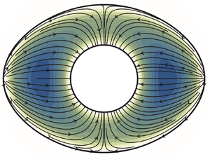
  $c$ defining the shape are selected to be those employed in the previous simulations (Carr et al. Reference Carr, Thomas, Liu and Shang2021), thereby facilitating comparison. Figure 3 shows the projection of the streamlines onto the tube section, i.e. the curves that are tangent to the transverse velocity $(v,w)=\dot {\mathcal {T}} (V,W)$. Since both transverse velocity components are proportional to the function $\dot {\mathcal {T}}(\kappa x'-\omega t')$, the resulting streamline pattern is independent of time and identical at all tube sections. The projected streamlines are perpendicular to the inner cylinder and tangent to the outer surface (except at the critical points $\theta =\theta _o$), a flow structure also revealed in the previous computations of Carr et al. (Reference Carr, Thomas, Liu and Shang2021).

Figure 3. The projection of the streamlines onto the cross-section of the tube obtained from integration of (5.1)–(5.5) for (a) an eccentric annulus with  $b=1.549$ and $c=0.349$, and (b) an elliptic annulus with $b=2$ and $c=1.2$ (see figure 2 for definition of $b$ and $c$); the colour contours represent the distribution of reduced axial velocity $U_o(r,\theta )$.
6. Tubes of finite length
Peristaltic motion in tubes of arbitrary length was first investigated by Li & Brasseur (Reference Li and Brasseur1993). Unlike the infinitely long tube, for which the single characteristic variable  $\xi =\kappa x'-\omega t'$ suffices to describe the temporal and streamwise dependence of the resulting periodic flow, for a tube of arbitrary finite length one needs to consider in general two different independent variables, because the solution is $2{\rm \pi}$-periodic in the rescaled time $t=\omega t'$ but non-periodic in the spatial variable $x=\kappa x'$. It is seen that the use of $\xi =\kappa x'-\omega t'$ and $t=\omega t'$ as independent variables facilitates the description of the flow rate $Q(\xi ,t)$ and pressure $p(\xi ,t)$.
The initial steps of the analysis leading to (4.1) parallel those presented above, with the pressure determined from
 \begin{equation} \frac{\partial}{\partial \xi} \left(-\frac{1}{{\mathcal{R}}} \frac{\partial {p}}{\partial \xi} \right)+2 {\rm \pi}(1+\varepsilon \mathcal{T}) \dot{\mathcal{T}}=0,\quad \left\{ \begin{array}{@{}l} {p}=0 \quad \textrm{at} \ \xi={-}t, \\ {p}=\delta{p}_L(t) \quad \textrm{at} \ \xi=\ell-t, \end{array} \right. \end{equation}
where  $\ell =\kappa L$ is the dimensionless tube length and $\delta p_L(t)=\delta p'_L/[\mu \varepsilon \omega /(\kappa r'_o)^2]$ is the dimensionless pressure difference between the inlet $x'=0$ ( $\xi =-t$) and the outlet $x'=L$ ( $\xi =\ell -t$). Integrating (6.1) once gives
 \begin{equation} Q={-}\frac{1}{\mathcal{R}} \frac{\partial p}{\partial \xi}=C_L(t)-2 {\rm \pi}(\mathcal{T} +\varepsilon \mathcal{T}^2/2), \end{equation}
involving the periodic function  $C_L(t)$. Multiplying by $\mathcal {R}$ and integrating a second time yields
 \begin{equation} C_L(t)=\frac{\displaystyle 2{\rm \pi} \int_{{-}t}^{\ell-t} \mathcal{T} \mathcal{R}\, \textrm{d}\xi+{\rm \pi} \varepsilon \int_{{-}t}^{\ell-t} \mathcal{T}^2 \mathcal{R}\, \textrm{d}\xi- \delta{p}_L(t)}{\displaystyle \int_{{-}t}^{\ell-t} \mathcal{R}\, \textrm{d}\xi} \end{equation}
after imposing the boundary conditions at both ends. As expected, since  $\mathcal {R}$, $\mathcal {T}$ and $\dot {\mathcal {T}}=\textrm {d} \mathcal {T}/\textrm {d} \xi$ are $2{\rm \pi}$-periodic functions of $\xi$, the expression (6.3) naturally reduces to (4.4) with $\delta p_\lambda =\delta p_L/j$ when $L$ is a multiple of the wavelength, so that $\ell =\kappa L=2 {\rm \pi}j$, with $j=1,2,3, \dots$. Substituting (6.3) into (6.2) provides the flow rate $Q(x,t)$, whose dependence on the streamwise coordinate $x$ enters through the wavefunction $\mathcal {T}(\xi )=\mathcal {T}(x-t)$. Taking the time average of (6.2) at any given section $x$ reveals that
 \begin{equation} \frac{1}{2 {\rm \pi}} \int_{0}^{2{\rm \pi} } Q \,\textrm{d} t=\langle C_L \rangle-\varepsilon {\rm \pi}\langle \mathcal{T}^2 \rangle \end{equation}
in terms of the mean value  $\langle C_L \rangle$.
The solution simplifies for small peristaltic amplitudes  $\varepsilon \ll 1$. Using (3.6) in (6.3), substituting the result into (6.2), and taking the time average gives, with small errors of order $\varepsilon ^2$,
 \begin{align} \frac{1}{2 {\rm \pi}} \int_{0}^{2{\rm \pi} } Q \,\textrm{d} t&={-}\frac{\langle \delta{p}_L
\rangle}{\ell \mathcal{R}_o}+2 {\rm \pi}
\varepsilon \varDelta \left[\vphantom{\left\langle
\left(\int_{{-}t}^{\ell-t} \mathcal{T} \,\textrm{d} \xi
\right)^2 \right\rangle}\langle \mathcal{T}^2
\rangle-\frac{1}{\ell^2} \left\langle
\left(\int_{{-}t}^{\ell-t} \mathcal{T} \,\textrm{d} \xi
\right)^2 \right\rangle \right. \nonumber\\ &\hspace{8.1pc} +\left.
\frac{1}{\ell} \left\langle \left( \int_{{-}t}^{\ell-t}
\mathcal{T} \,\textrm{d}\xi \right) \frac{\delta
p_L}{2{\rm \pi} \mathcal{R}_o \ell} \right\rangle \vphantom{\left\langle
\left(\int_{{-}t}^{\ell-t} \mathcal{T} \,\textrm{d} \xi
\right)^2 \right\rangle}\right]
\end{align}
\begin{align} \frac{1}{2 {\rm \pi}} \int_{0}^{2{\rm \pi} } Q \,\textrm{d} t&={-}\frac{\langle \delta{p}_L
\rangle}{\ell \mathcal{R}_o}+2 {\rm \pi}
\varepsilon \varDelta \left[\vphantom{\left\langle
\left(\int_{{-}t}^{\ell-t} \mathcal{T} \,\textrm{d} \xi
\right)^2 \right\rangle}\langle \mathcal{T}^2
\rangle-\frac{1}{\ell^2} \left\langle
\left(\int_{{-}t}^{\ell-t} \mathcal{T} \,\textrm{d} \xi
\right)^2 \right\rangle \right. \nonumber\\ &\hspace{8.1pc} +\left.
\frac{1}{\ell} \left\langle \left( \int_{{-}t}^{\ell-t}
\mathcal{T} \,\textrm{d}\xi \right) \frac{\delta
p_L}{2{\rm \pi} \mathcal{R}_o \ell} \right\rangle \vphantom{\left\langle
\left(\int_{{-}t}^{\ell-t} \mathcal{T} \,\textrm{d} \xi
\right)^2 \right\rangle}\right]
\end{align}
for the time-averaged flow rate. As expected, the above equation reduces to (4.5) for  $\ell =2{\rm \pi} j$, when $\delta {p}_L=j \delta {p}_\lambda$ and $\int _{-t}^{\ell -t} \mathcal {T} \,\textrm {d} \xi =0$. For a sinusoidal wave $\mathcal {T}=\sin \xi$ in a tube with equal pressure at both ends, (6.5) reduces to
 \begin{equation} \frac{1}{2 {\rm \pi}} \int_{0}^{2{\rm \pi} } Q \,\textrm{d} t={\rm \pi} \varepsilon \varDelta [1-2(1-\cos \ell)/\ell^2], \end{equation}
to be compared with the result  $\int _{0}^{2{\rm \pi} } Q\, \textrm {d} t/(2{\rm \pi} )={\rm \pi} \varepsilon \varDelta$ obtained earlier for an infinitely long tube. The comparison indicates that the effect of non-integral length $\ell \ne 2{\rm \pi} j$ is to reduce the level of pumping, in agreement with previous findings (Li & Brasseur Reference Li and Brasseur1993).
7. Conclusions
A complete analytical description has been given for the lubrication flow induced in non-axisymmetric tubes by a periodic wave propagating axially along its inner surface, assumed to be a circular cylinder. The explicit expressions derived for the pumping rate, involving the dimensionless hydraulic resistance  $\mathcal {R}_o$ and its relative variation in response to changes of the inner radius $\varDelta$, can be used to assess the role of peristaltic pumping in applications involving transport along asymmetric annuli. In particular, the results given in § 6 can in principle be used in connection with the problem of CSF flow in the perivascular system, with the overall network of perivascular spaces surrounding arteries assumed to be composed of multiple peristaltic elements of length $L$ – possibly different for different elements – connected at bifurcating nodes. Since the wavelength $2 {\rm \pi}/\kappa$ of the arterial pulsations is very large compared with the length $L$ of each peristaltic element, the expression given above in (6.5) for the relation between $\delta {p}_L$ and $Q$ could be simplified by using the limit $\ell =\kappa L \ll 1$. Combining the $\delta {p}_L$– $Q$ relation corresponding to the different peristaltic elements with the continuity condition at each bifurcating node provides a set of equations that determine the distribution of flow and pressure throughout the periarterial system. Simplified computational approaches like this can be instrumental in understanding the overall features of CSF flow, complementing on-going efforts (Ladrón-de-Guevara et al. Reference Ladrón-de-Guevara, Shang, Nedergaard and Kelley2021).
Funding
This work was supported by the National Science Foundation through grant number 1853954. W.C. acknowledges partial support from the ‘Convenio Plurianual Comunidad de Madrid – Universidad Carlos III de Madrid’ through grant CSFLOW-CM-UC3M.
Declaration of interests
The authors report no conflict of interest.


 Open access