


1. Introduction
The study of thin-layer vortex dynamics has long provided insight into the complex behaviour of shear layers, jets and wakes. In particular, vortex sheets provide a simple model for infinitely thin shear layers (Moore Reference Moore1978; Baker & Shelley Reference Baker and Shelley1990; Dhanak Reference Dhanak1994; Caflisch, Lombardo & Sammartino Reference Caflisch, Lombardo and Sammartino2020). However, like most long-wave approximations, difficulties arise in the behaviour of the small scales, in this case the presence of the Kelvin–Helmholtz instability. Moore (Reference Moore1979) provides plausible evidence that an initially straight vortex sheet subject to a small-amplitude initial disturbance develops a curvature singularity in a finite (critical) time proportional to the logarithm of the inverse disturbance amplitude. Supporting evidence comes from direct numerical simulations (Krasny Reference Krasny1986b; Shelley Reference Shelley1992), from Taylor series expansions in time (Meiron, Baker & Orszag Reference Meiron, Baker and Orszag1982) and from asymptotic studies (Caflisch & Semmes Reference Caflisch and Semmes1990; Cowley, Baker & Tanveer Reference Cowley, Baker and Tanveer1999). A clear picture emerges of the formation of a curvature singularity in the vortex sheet as a consequence of the presence of 3/2-power singularities in the complex plane of the Lagrangian marker that reach the real axis in finite time.
Of course, interest has turned to understanding the nature of the vortex sheet after the singularity time. Rigorous mathematics (Delort Reference Delort1991; Majda Reference Majda1993) has established global existence for vortex sheet motion in the classic weak sense, but the details of the weak solution are elusive. Wu (Reference Wu2006) demonstrates that the weak solution is not simple; indeed even a logarithmic spiral does not qualify. The most likely access to identifying the weak solution is through the limit of an appropriate sequence of approximate solutions to the Euler equations (Majda & Bertozzi Reference Majda and Bertozzi1992) and the most common choice is the vortex-blob approximation (Krasny Reference Krasny1986a). Unfortunately, the limit of zero blob size still contains several mysteries (Baker & Pham Reference Baker and Pham2006); in particular, the arms of the spiral lie within an area of overlapping blob size and the spiral appears to collapse to a point in the limit of zero blob size (Baker & Pham Reference Baker and Pham2006).
An alternative shear-layer model can be constructed from thin strips or infinitely long patches of initially spatially uniform vorticity. Since in two-dimensional incompressible inviscid Euler flow vorticity is conserved following a material particle, the vorticity remains uniform in the subsequent patch motion, allowing a dimensional reduction where the two-space-dimensional patch dynamics can be contracted to one-dimensional integro-differential equations that describe the evolution of the patch boundaries or contours (Zabusky, Hughes & Roberts Reference Zabusky, Hughes and Roberts1979), an approach often described as ‘contour dynamics’ (see Pullin (Reference Pullin1992) for a review). An important property of this model is that the motion exists globally in time (Yudovich Reference Yudovich1963), while if the initial boundaries are smooth, they remain smooth for all time (Chemin (Reference Chemin1993); see Majda & Bertozzi (Reference Majda and Bertozzi1992) for a review).
For a single vortex layer, in the limit where the vorticity magnitude becomes large and the layer thickness becomes small with the constraint that their product remains finite, the uniform vorticity strip will converge to a vortex sheet (Majda & Bertozzi Reference Majda and Bertozzi1992). Because the motion of the vortex patch exists for all time, a study of the limit provides a different, physically based, approach to understanding the nature of the vortex sheet after the singularity time. Moore (Reference Moore1978) explored the small-thickness limit using the method of matched asymptotic expansions, obtaining a modified version of the Birkhoff–Rott (BR) equation (Rott Reference Rott1956; Birkhoff Reference Birkhoff1962) that describes the motion of a vortex sheet in two-dimensional flow. A difficulty with the theory is that short waves are unstable with growth rates that are even faster than Kelvin–Helmholtz (square of the wavenumber). Moore points out that while such waves lie outside the validity of the theory, their presence in a numerical calculation will lead to numerical difficulties similar to those encountered in vortex sheet calculations.
The limit dynamics for thin vortex layers has been further studied by Baker & Shelley (Reference Baker and Shelley1990), Dhanak (Reference Dhanak1994) and Caflisch et al. (Reference Caflisch, Lombardo and Sammartino2020). Moore's result is extended by Dhanak (Reference Dhanak1994) to a higher order, who still finds the presence of spurious short-wave instabilities. Numerical solutions by Baker & Shelley (Reference Baker and Shelley1990) for a single uniform vortex layer reveal interesting differences between vortex sheet and thin-vortex-layer dynamics. While a perturbed vortex sheet shows the inevitable formation of a curvature singularity, a thin vortex layer develops an elliptical core at the centre of roll-up whose size and total circulation content, at a given time, reduces with reducing initial layer thickness. Within the core a material curve that initially coincided with the layer's centre curve forms a double-branched spiral. The appearance of these structures invalidates assumptions in the analytical small-thickness approximation, but are in accord with the suggestions by Wu (Reference Wu2006) that the weak limit is not simple. These thin-layer numerical simulations bear some resemblance to the so called  $\delta$-regularization (Krasny Reference Krasny1986a) of the BR equation that allows numerical computation of vortex-sheet-like evolution beyond the critical time.
Thin vortex layers with general vorticity distributions have received less attention. The main result, due to Caflisch et al. (Reference Caflisch, Lombardo and Sammartino2020), establishes the existence of a vortex layer structure for short times. The thin layer is assumed to be O( $\epsilon$) wide – vorticity decays exponentially along a distance normal to a centre curve – with vorticity intensity $O(1/\epsilon )$; its motion is well described by a modified BR equation. The approximate equations of motion are rather intricate and it is difficult to assess the consequences.
Instead of a smooth vorticity distribution considered by Caflisch et al. (Reference Caflisch, Lombardo and Sammartino2020), we consider a thin vortex layer composed of two adjacent strips of uniform, but possibly different, vorticity. By adapting the techniques of contour dynamics, the motion of the layer may be described in terms of three integrals, one each on the boundaries of the layer and one on the interface that separates the vortex strips. These integrals may be expanded in a layer-thickness parameter, leading to a set of evolution equations that have the appearance of a modified BR equation and with clear analogies to the results of Caflisch et al. (Reference Caflisch, Lombardo and Sammartino2020). The system that emerges is four coupled integro-differential equations with a simple form, suggesting several new avenues of research.
Krasny (Reference Krasny1989) constructed a two-dimensional model for a wake flow comprised of a vortex sheet combined with a dipole sheet whose evolution is governed by an equation adapted from the transport equation for the gradient of the vorticity in a continuous vorticity field, but details are not provided. Desingularized numerical simulations show the development of wake-like flow patterns. While complex dipole distributions in the sense of potential theory (Jaswon & Symm Reference Jaswon and Symm1977) are used in the development below to derive equations of motion for the double vortex layer, the normal component of a vortex dipole distribution does not appear in the limiting velocity equation. (Appendix A clarifies the properties of tangential and normal components of vortex dipole distributions, and shows that these two components correspond to real and imaginary vortex sheet strengths, respectively.)
The results of a linear stability analysis for the two-layer system appear in Pozrikidis & Higdon (Reference Pozrikidis and Higdon1987). In general, the layers are susceptible to the Kelvin–Helmholtz instability, as expected, and this instability is present in the thin-layer equations. The exception, of course, is when there is no mean shear across the layers. While layers of finite thickness still exhibit instability, the growth rates are very small for very thin layers. Indeed, the thin-layer equations exhibit only a linear growth in time, a result that can only be established by a full stability analysis based on an initial-value calculation. These results open up the possible long-time existence of sufficiently thin layers.
The organization of the paper is as follows. The flow is defined in § 2 and general equations of motion are derived. Expansions in a layer-thickness parameter for thin layers are developed in § 3. These are used to develop leading-order thin-layer equations for the two-layer system in § 4. Special attention is given to the case of the circulation-free layer. Analysis of the linearized stability behaviour of the thin-double-layer equations is given in § 5. A discussion and conclusions are presented in § 6, while asymptotic expansions for integrals and the interface velocities are outlined in Appendices B and C.
2. The equations of motion for a double layer
2.1. Flow configuration
Figure 1 is a companion to figure 2 of Baker & Shelley (Reference Baker and Shelley1990). In Cartesian coordinates  $(x,y)$ with $x$ streamwise, this shows adjacent double vortex layers, each of uniform vorticity, that extend to infinity in either $x$ direction. The defining, constant parameters are the layer mean thicknesses $H_1>0$, $H_2>0$; the fluid $x$ velocities at $y \to \pm \infty$ are $U_2$ and $U_1$, respectively. Regions $R_{-\infty }$, $R_1$, $R_2$ and $R_\infty$ denote, respectively, the irrotational fluid below, extending to $y\to -\infty$, the bottom and top vortex layers and the irrotational fluid above extending to $y\to \infty$. In these regions the uniform vorticities are respectively $\omega _{-\infty }=0$, $\omega _1 = U_1/H_1$, $\omega _2 = -U_2/H_2$ and $\omega _\infty =0$. The three bounding curves that make vorticity discontinuities are denoted $C_j$, $j=1,0,2$, whose shapes are described by the corresponding complex functions
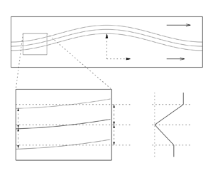
  $z_j(p,t)$. This choice of flow configuration is motivated as a model for the boundary layers shed on either side of an infinitely thin splitter plate.

Figure 1. An illustration of the asymptotic assumptions for a thin double layer. The bottom-left panel shows a zoomed-in version of the layer with the regions  $R_i$ indicated. The thicknesses $h_i$ are also given, along with the mean thicknesses $H_i$. The bottom-right panel shows the velocity profile corresponding to the mean layer thicknesses when the interface is flat.
The stream function  $\psi (x,y,t)$ satisfies Poisson equations in each region:
 \begin{equation} \nabla^{2} \psi = \begin{cases} 0 & \text{in $R_{-\infty}$} , \\ -U_1/H_1 & \text{in $R_1$}, \\ U_2/H_2 & \text{in $R_2$}, \\ 0 & \text{in $R_\infty$}. \end{cases}\end{equation}
A particular solution  $\bar {\psi }$ is generated by the case of flat interfaces defined by $z_1 =p+ U_1 t - {{\rm i}}H_1$, $z_0=p$ and $z_2 = p+U_2,t + {{\rm i}}H_2$, where $p$ is a Lagrangian marker, with the requirement that the stream function and its normal derivative be continuous at each interface:
 \begin{equation} \bar{\psi} = \begin{cases} U_1 y + U_1 H_1/2 & \text{in $R_{-\infty}$}, \\ -U_1y^{2}/(2H_1) & \text{in $R_1$}, \\ U_2y^{2}/(2H_2) & \text{in $R_2$}, \\ U_2 y - U_2 H_2/2 & \text{in $R_\infty$}, \end{cases}\end{equation}
where constants have been chosen to make the  $x$ velocity in $R_{-\infty }$ equal to $U_1$ and that in $R_\infty$ equal to $U_2$. The fluid velocity on $z_0$ is then zero. The general solution is $\psi = \bar {\psi } + \tilde {\psi }$, where $\tilde {\psi }$ satisfies the homogeneous equation
 \begin{equation} \nabla^{2} \tilde{\psi} = 0\end{equation}
in all regions. Here  $\tilde {\psi }$ must satisfy certain jump conditions at the interfaces to ensure the continuity of $\psi$ and its normal derivative.
2.2. Complex velocity
Define  $\varPsi = \tilde {\psi } - {{\rm i}} \tilde {\phi }$ and $\eta = x + {{\rm i}}y$. Then the complex stream function $\varPsi ( \eta )$ is analytic in all regions, and $\tilde {\phi }$ is a velocity potential. The complex velocity, $w = u + {{\rm i}}v$, is given by
 \begin{equation} w^{*} = \frac{{{\rm d}} \bar{\psi}}{{{\rm d}}y} + {{\rm i}} \frac{{{\rm d}} \varPsi}{{{\rm d}} \eta}, \end{equation}
where the star superscript indicates complex conjugation. Since  ${{\rm d}} \varPsi /{{\rm d}} \eta$ must vanish as $y \rightarrow \pm \infty$, $\varPsi$ can be represented by a distribution of complex dipoles $\varLambda _j$ (Jaswon & Symm Reference Jaswon and Symm1977) along each interface $C_j$:
 \begin{equation} \varPsi ( \eta ) = \sum_{ j=0}^{2} \int_{C_j} \varLambda_j (q) K ( \eta, z_j (q) ) z_{j,q} (q)\, {{\rm d}}q, \end{equation}
where the subscript  $q$ indicates differentiation with respect to $q$ and
 \begin{equation} K ( \eta , z ) = \frac{1}{2{\rm \pi} {{\rm i}}} \frac{1}{ \eta - z}.\end{equation}
An important property of  $K(\eta,z)$ arises when the complex dipole strength is constant, $\varLambda =1$ for example:
 \begin{equation} 2 \int K( \eta ,z(q)) z_q (q)\, {{\rm d}}q = \begin{cases} -1, & \text{$\eta$ above interface}, \\ 0 , & \text{$\eta$ on interface and the principal value is taken}, \\ 1, & \text{$\eta$ below interface} . \end{cases}\end{equation}
This result is part of a more general result concerning the limiting values of the stream function as the field point  $\eta$ approaches the surface at $z(q)$ along its normal. Letting $\eta \rightarrow z_1 (p)$ along the normal to $C$ from below, we may indent the contour: this procedure is akin to the derivation of the Plemelj formulae. The integral is split into two parts: the interface without the semicircle which leads to a principal-valued integral and the semicircular part which leads to a half-residue contribution. Following this procedure from both above and below the interface and letting $\psi ^{(\pm )}$ be the respective limiting values for the stream function, we have
 \begin{equation} \varPsi^{({\pm})}(z(p)) ={\pm} \frac{1}{2} \frac{\varLambda_p}{z_p} + {\int\hskip -1,05em -\,}_C \varLambda(q) K(z(p),z(q))z_q \, {{\rm d}}q,\end{equation}
where the stroke indicates that the Cauchy principal value must be taken.
The complex dipole distributions for  $\varPsi$ (2.5) lead to the contribution to the complex conjugate of the velocity:
 \begin{equation} \frac{{{\rm d}} \varPsi}{{{\rm d}} \eta} ( \eta ) = \sum_{j=0}^{2} \int_{C_j} \varLambda_{j,q} (q) K ( \eta , z_j (q)) \, {{\rm d}}q,\end{equation}
where an integration by parts has been done, based on the relation
 \begin{equation} \frac{{{\rm d}}}{{{\rm d}} \eta} K( \eta , z_j (q)) z_{j,q} (q) ={-} \frac{{{\rm d}}}{{{\rm d}}q} K( \eta , z_j (q)). \end{equation}
 The derivatives of the complex dipole strength,  $\varLambda _{j,q} (q)$, are determined by requiring continuity of velocity at $C_j$. The limiting values of the complex velocity jump across an interface can be determined by (2.8). Consider the lower interface $C_1$ as an example:
 \begin{align} \frac{{{\rm d}} \varPsi^{({\pm})}}{{{\rm d}} \eta} (p) &={\pm}\frac{1}{2} \frac{\varLambda_{1,p} (p)}{z_{1,p} (p)} + {\int\hskip -1,05em -\,}_{C_1} \varLambda_{1,q} (q) K (z_1 (p),z_1 (q))\, {{\rm d}}q \nonumber\\ &\quad + \int_{C_0} \varLambda_{0,q} (q) K (z_1 (p),z_0 (q))\, {{\rm d}}q+ \int_{C_2} \varLambda_{2,q} (q) K(z_1 (p),z_2 (q))\, {{\rm d}}q. \end{align}
Continuity of velocity at the interface  $C_1$ then requires that
 \begin{equation} \frac{{{\rm d}} \bar{\psi}^{(+)}}{{{\rm d}}y} (p) + {{\rm i}} \frac{{{\rm d}} \varPsi^{(+)}}{{{\rm d}} \eta} (p) = \frac{{{\rm d}} \bar{\psi}^{(-)}}{{{\rm d}}y} (p) + {{\rm i}} \frac{{{\rm d}} \varPsi^{(-)}}{{{\rm d}} \eta} (p) , \end{equation}
and so
 \begin{equation} \varLambda_{1,p} (p) = {{\rm i}}U_1 \left(1 + \frac{y_1 (p)}{H_1} \right) z_{1,p} (p). \end{equation}
Similarly, continuity of velocity at the interface  $C_2$ implies that
 \begin{equation} \varLambda_{2,p} (p) ={-}{{\rm i}}U_2 \left( 1 - \frac{y_2(p)}{H_2}\right) z_{2,p} (p). \end{equation}
On the middle interface  $C_0$,
 \begin{equation} \varLambda_{0,p} (p) ={-} {{\rm i}} \left( \frac{U_1}{H_1}+\frac{U_2}{H_2}\right) y_0(p) z_{0,p}. \end{equation}
From (2.2), (2.4) and (2.13), the complex conjugate of the velocity may be determined anywhere in the fluid.
A convenient form for the velocity may be obtained by using (2.7). The complex fluid velocity is given in the compact form
 \begin{align} w^{*}( \eta ) &= \frac{U_1+U_2}{2} - \frac{U_1}{H_1} \int_{C_1} (y_1 (q) - y )) K( \eta ,z_1 (q)) z_{1,q} (q)\, {{\rm d}}q \nonumber\\ &\quad - \frac{U_2}{H_2} \int_{C_2} (y_2 (q) - y ) K( \eta ,z_2 (q)) z_{2,q} (q)\, {{\rm d}}q \nonumber\\ &\quad + \left(\frac{U_1}{H_1}+\frac{U_2}{H_2}\right) \int_{C_0} (y_0(q)-y) K(\eta, z_0(q)) z_{0,q}(q)\, {{\rm d}}q. \end{align}
This result is an obvious extension of the complex velocity in Baker & Shelley (Reference Baker and Shelley1990).
2.3. Equations of motion
Since the interfaces must move with the fluid velocity, their equations of motion are
 $$\begin{gather} \frac{\partial z_0}{\partial t} (p,t) = w_0 (p,t) \equiv w( z_0(p,t)), \end{gather}$$
 $$\begin{gather}\frac{\partial z_1}{\partial t} (p,t) = w_1 (p,t) \equiv w (z_1 (p,t)), \end{gather}$$
 $$\begin{gather}\frac{\partial z_2}{\partial t} (p,t) = w_2 (p,t) \equiv w (z_2 (p,t)), \end{gather}$$
where the partial time derivatives are taken keeping the Lagrangian variable,  $p$, fixed.
The equations of motion may be transformed to any frame of reference moving with uniform velocity in the  $x$ direction. For example, resetting
 \begin{equation} z_j \rightarrow -\frac{U_1+U_2}{2} t + z_j, \quad w \rightarrow -\frac{U_1+U_2}{2} + w, \end{equation}
then the far-field velocities become
 \begin{equation} w \rightarrow \frac{U_2-U_1}{2} \text{ as $y \rightarrow \infty$}, \quad w \rightarrow \frac{U_1-U_2}{2} \text{ as $y\rightarrow -\infty$}. \end{equation}
There are two particular situations of interest. Set  $U_2=U$ and $U_1=-U$ with $H_1=H_2=H/2$ and the result is just the same as for the single layer (Baker & Shelley Reference Baker and Shelley1990). This result may be used as a check on the expansions for the double layer. The case more relevant to double layers is $U_1=U_2=U$. Effectively, the mean vortex sheet strength has been set to zero so focus can be placed on the effects of the internal structure of the double layer.
3. Expansions for small thickness
In this section, the evolution of thin vortex layers is studied in the limit as their thicknesses tend to zero. At any fixed time, the two exterior interfaces  $C_1, C_2$ will collapse onto the central interface $C_0$ in this limit. As a starting point for the analysis of the behaviour of thin layers, the exterior interfaces may be considered to lie a short distance on either side of the central interface. However, the Lagrangian motion of points on the exterior curves will result in their displacement tangentially to the limiting curve. Consequently, the use of a parametrization based on Lagrangian motion is inconvenient. Instead, a new parametrization is introduced to ensure that points on the exterior interfaces with the same label will converge to the same point on the central interface. The idea is to express the exterior interfaces in terms of their distance along the normal to the central interface. The definition for the motion of points on the exterior interfaces must be modified so that a point on either exterior interface normal to a particular point on the central interface will remain so subsequently.
3.1. Parametrization of exterior vorticity interfaces
The exterior interfaces are assumed to have the form
 $$\begin{gather} z_1 (p) = z_0 (p) - {{\rm i}}h_1 (p) \frac{z_{0,p} (p)}{s_{0,p} (p)}, \end{gather}$$
 $$\begin{gather}z_2 (p) = z_0 (p) + {{\rm i}}h_2 (p) \frac{z_{0,p} (p)}{s_{0,p} (p)}, \end{gather}$$
where  $s_{0,p} = | z_{0,p} |$ for which the subscript $p$ refers to differentiation. The real functions $h_1(p)$ and $h_2(p)$ give the distance of the exterior interfaces to the central interface $z_0(p)$ along its normal and are assumed to be smooth.
The parametrization of the central curve  $z_0(p)$ is valid provided it has a derivative $z_{0,p}$ such that $s_{0,p} = |z_{0,p}|$ is always positive and is never zero; the requirement is equivalent to demanding the existence of a smooth tangent. The validity of the parametrization for the exterior surfaces depends on the smoothness of the distances $h_1(p)$ and $h_2(p)$, but also on the properties of the centre curve. In general, we require the derivatives of $z_1$ and $z_2$ to be also well defined. The derivatives may be written as
 $$\begin{gather} \frac{z_{1,p}}{s_{0,p}} = \left[ 1 -{{\rm i}} \frac{h_{1,p}}{{s_{0,p}}} +h_1 \kappa \right] \frac{z_{0,p}}{s_{0,p}}, \end{gather}$$
 $$\begin{gather}\frac{z_{2,p}}{s_{0,p}} = \left[ 1 +{{\rm i}} \frac{h_{2,p}}{s_{0,p}} -h_2 \kappa \right] \frac{z_{0,p}}{{s_{0,p}}}, \end{gather}$$
where
 \begin{equation} \kappa = \frac{x_{0,p} y_{0,pp}-y_px_{0,pp}}{s_{0,p}^{3}}\end{equation}
is the curvature of the centre curve.
The parametrization for the external surfaces can fail under several different possibilities. Assume the centre curve is well defined;  $z_{0,p}/s_{0,p}$ (tangent) exists. Then it is the quantities $h_p/s_p$ and $h\kappa$ that matter; here $h$ stands for either $h_1$ or $h_2$.
(i) If $h_p$ blows up then it is a possible signal that the external surface folds over itself. If this is the case, then $h$ becomes multivalued and the limit of a thin layer does not make sense. Note that the contour dynamics equations do allow for bounding surfaces to fold over but the parametrization will be different from (3.1).
(ii) If the curvature is too large, then it is possible that there are places where
$\Re \{z_{1,p}\}=0$ or $\Re \{z_{2,p}\}=0$ and the bounding surface may loop around on itself. This is akin to the inability to extend the normal away from the centre curve without crossing itself.(iii) Finally, we require
$1 - {{\rm i}}h_p/s_p +h \kappa \neq 0$. This condition is more difficult to phrase in simple geometric terms.


To avoid these potential difficulties, the long-wave limit will require both  $h_p/s_p$ and $h\kappa$ to be small. We also assume that $h$ remains positive.
3.2. Motion with new parametrization
The motion of a point, labelled by  $p$, on one of the exterior interfaces, labelled by $j$, will no longer be with the fluid flow. Let $w_j (p)$ be the fluid velocity at that point; $w_j (p) = w ( z_j (p) )$. Then the motion of the point will be given by
 \begin{equation} \frac{\partial z_j}{\partial t} (p) = w_j (p) + \alpha_j (p) \frac{z_{j,p} (p)}{ s_{j,p} (p)}, \quad \text{for $j=1,2$},\end{equation}
where  $\alpha _j(p)$ is a real function controlling the speed that must be added to the fluid velocity along the tangent to the exterior interface so that the point remains on the normal to the internal curve at $z_0(p)$. The motion in the normal direction of any point on the bounding curves will be that of the fluid for kinematic reasons.
The substitution of (3.1) into (3.4) gives two complex equations:
 $$\begin{gather} {{\rm i}} \frac{\partial h_1} {\partial t} \frac{z_{0,p}} {s_{0,p}} - h_1 \Im \left\{\frac{w_{0,p}} {z_{0,p}} \right\} \frac{z_{0,p}} {s_{0,p}} + w_1 - w_0 + \alpha_1 \frac{z_{1,p}} {s_{1,p}} = 0, \end{gather}$$
 $$\begin{gather}{{\rm i}} \frac{\partial h_2} {\partial t} \frac{z_{0,p}} {s_{0,p}} - h_2 \Im \left\{\frac{w_{0,p}} {z_{0,p}} \right\} \frac{z_{0,p}} {s_{0,p}} - w_2 + w_0 - \alpha_2 \frac{z_{2,p}} {s_{2,p}} = 0, \end{gather}$$
where  $w_0$ is the velocity of $z_0$. Dependence on $p$ will no longer be shown unless important. Given $h_1$, $h_2$ and $z_0$, the location of the exterior interfaces $z_1$ and $z_2$ are known, and the velocities $w_0$, $w_1$ and $w_2$ may be calculated by (2.15). Then (3.5) are two complex equations for the four real unknowns $\partial h_1/\partial t$, $\partial h_2/\partial t$, $\alpha _1$ and $\alpha _2$. Thus $h_1$ and $h_2$ may be advanced and the location of the central interface $z_0$ updated by (2.15a).
3.3. Thin-layer expansion
For double layers with mean thickness  $H=H_1+H_2$, the following expansions are assumed. For $j=1,2$:
 $$\begin{gather} h_j (p) = h_{j,1} (p) H + h_{j,2} (p) H^{2} + O ( H^{3} ), \end{gather}$$
 $$\begin{gather}\alpha_j (p) = \alpha_{j,0} (p) + \alpha_{j,1} (p) H + {O} ( H^{2}), \end{gather}$$
 $$\begin{gather}w_j (p) = w_{j,0} (p) + w_{j,1} (p) H + O ( H^{2} ). \end{gather}$$
For the central interface, assume
 $$\begin{gather} z_0 (p) = z(p) + \hat{z}_1 (p) H + \hat{z}_2 (p) H^{2} + O ( H^{3} ), \end{gather}$$
 $$\begin{gather}w_0 (p) = w (p) + \hat{w}_1 (p) H + O ( H^{2} ). \end{gather}$$
The above expansions (3.6) are substituted into (3.1) to give
 $$\begin{gather} z_1 = z + \left( \hat{z}_1 - {{\rm i}}h_{1,1} \frac{z_p}{s_p} \right) H + \left( \hat{z}_2 -{{\rm i}}h_{1,2} \frac{z_p}{s_p} + h_{1,1} \Im \left\{ \frac{\hat{z}_{1,p}}{z_p}\right\} \frac{z_p}{s_p} \right) H^{2} +O (H^{3}), \end{gather}$$
 $$\begin{gather}z_2 = z + \left( \hat{z}_1 + {{\rm i}}h_{2,1} \frac{z_p}{s_p} \right) H + \left( \hat{z}_2 +{{\rm i}}h_{2,2} \frac{z_p}{s_p} - h_{2,1} \Im \left\{ \frac{\hat{z}_{1,p}}{z_p}\right\} \frac{z_p}{s_p} \right) H^{2} +O (H^{3}). \end{gather}$$
 Now (3.6) and (3.7) are substituted into (3.5) and the collection of terms with equal powers in  $H$ are set to zero. For the first two orders,
 $$\begin{gather} w_{1,0} - w + \alpha_{1,0} \frac{z_p}{s_p} = 0, \end{gather}$$
 $$\begin{gather}w_{2,0} - w + \alpha_{2,0} \frac{z_p}{s_p} =0, \end{gather}$$
and
 $$\begin{gather} w_{1,1} - \hat{w}_1 + \frac{z_p}{s_p} \left[\alpha_{1,1} + {{\rm i}} \frac{\partial h_{1,1}}{\partial t} - h_{1,1} \Im \left\{ \frac{w_p}{z_p} \right\} - {{\rm i}} \alpha_{1,0} \left( \frac{h_{1,1,p}}{s_p} - \Im \left\{ \frac{\hat{z}_{1,p}}{z_p} \right\} \right) \right] = 0, \end{gather}$$
 $$\begin{gather}w_{2,1} - \hat{w}_1 + \frac{z_p}{s_p} \left[\alpha_{2,1} - {{\rm i}} \frac{\partial h_{2,1}} {\partial t} + h_{2,1} \Im \left\{ \frac{w_p}{z_p} \right\} + {{\rm i}} \alpha_{2,0} \left( \frac{h_{2,1,p}}{s_p} + \Im \left\{ \frac{\hat{z}_{1,p}}{z_p} \right\} \right) \right] = 0. \end{gather}$$
 The next step is the substitution of (3.6) into (2.15) to provide relationships between the coefficients of the expansion for  $w_j$ and those for $z_0$. The complex velocity at the interfaces depends on integrals of the form
 \begin{equation} I_{j,k} (p) = \frac{1}{2{\rm \pi} {{\rm i}}} \int \frac{ y_k (q) - y_j (p) }{ z_j (p) - z_k (q)} z_{k,q} (q)\, {{\rm d}}q. \end{equation}
The expansions of these integrals for each  $w_j$ are derived in Appendix C.
3.4. Functions $\varGamma$ and $T$


First, introduce the quantities
 $$\begin{gather} T_1(p) = \left(\frac{U_1 h_{1,1}}{H_1} + \frac{U_2 h_{2,1}}{H_2} \right) H , \end{gather}$$
 $$\begin{gather}T_2(p) = \left(\frac{U_1 h_{1,2}}{H_1} + \frac{U_2 h_{2,2}}{H_2} \right) H , \end{gather}$$
 $$\begin{gather}\varGamma_1(q) = \left(\frac{U_1 h_{1,1}}{H_1} - \frac{U_2 h_{2,1}}{H_2} \right) H , \end{gather}$$
 $$\begin{gather}\varGamma_2(q) = \left(\frac{U_1h_{1,2}}{H_1} - \frac{U_2 h_{2,2}}{H_2}\right) H . \end{gather}$$
From (C8),
 $$\begin{gather} w^{*} = \frac{U_1+U_2}{2} -\frac{T_1(p) }{2} \frac{z_p^{*}}{s_p} +\frac{1}{2{\rm \pi} {{\rm i}}} {\int\hskip -1,05em -\,} \frac{\varGamma_1(q)s_q}{z(p)-z(q)}\, {{\rm d}}q, \end{gather}$$
 $$\begin{gather}\hat{w}_1^{*} = P_2^{(0)} + \frac{1}{2{\rm \pi} {{\rm i}}} {\int\hskip -1,05em -\,} \frac{\tau_2^{(0)} z_q}{z(p)-z(q)}\, {{\rm d}}q, \end{gather}$$
where  $P_2^{(0)}$ and $\tau _2^{(0)}$ are defined in (C10) and (C11). From (C17),
 $$\begin{gather} w^{*}_{1,0} = \frac{U_1+U_2}{2} +\frac{\varGamma_1(p)}{2} \frac{z^{*}_p}{s_p}+\frac{1}{2{\rm \pi} {{\rm i}}} {\int\hskip -1,05em -\,} \frac{\varGamma_1(q) s_q }{z(p)-z(q)} \,{{\rm d}}q, \end{gather}$$
 $$\begin{gather}w_{1,1}^{*} = P_2^{(1)} + \frac{1}{2{\rm \pi} {{\rm i}}} \int \frac{\tau_2^{(1)}(q) z_q}{z(p)-z(q)}\, {{\rm d}}q, \end{gather}$$
where  $P_2^{(1)}$ and $\tau _2^{(1)}$ are defined in (C19) and (C20). From (C26),
 $$\begin{gather} w^{*}_{2,0} = \frac{U_1+U_2}{2} - \frac{\varGamma_1(p)}{2} \frac{z^{*}_p}{s_p}+\frac{1}{2{\rm \pi} {{\rm i}}} {\int\hskip -1,05em -\,} \frac{\varGamma_1(q) s_q }{z(p)-z(q)} \, {{\rm d}}q, \end{gather}$$
 $$\begin{gather}w_{2,1}^{*} = P_2^{(2)} + \frac{1}{2{\rm \pi} {{\rm i}}} {\int\hskip -1,05em -\,} \frac{\tau_2^{(2)}(q) z_q}{z(p)-z(q)}\, {{\rm d}}q, \end{gather}$$
where  $P_2^{(1}$ and $\tau _2^{(1)}$ are defined in (C28) and (C29).
4. Limiting equations of motion
Before examining the limiting equations, it is worth understanding the connection between the local thicknesses  $h_j$ and the mean thicknesses $H_j$. This is most easily obtained by considering the conservation of area of the two layers separately. The first step is to establish a horizontal length scale. To that end, let $P$ be the value of parameter such that
 \begin{equation} L = \int_{{-}P}^{P} x_{0,p}\, {{\rm d}}p.\end{equation}
 In what follows, we consider the layer to be periodic with length  $L$, or that the layer becomes flat as $p\rightarrow \pm \infty$. Then, the area of a segment of the lower layer (region $R_1$) is
 \begin{equation} A_1 = \int_{{-}P}^{P} [ y_0(p) x_{0,p}(p) - y_1(p)x_{1,p}(p)] \,{{\rm d}}p = H_1L. \end{equation}
This statement may be interpreted as the definition of the mean thickness of the layer in region  $R_1$ where either $L$ is the periodic length, or the limit $L\rightarrow \infty$ is taken. To lowest order, the areas of both layers become
 \begin{equation} A_1 = H \int _{{-}P}^{P} h_{1,1} s_p \, {{\rm d}}p =H_1L, \quad A_2 = H \int_{{-}P}^{P} h_{2,1} s_p\, {{\rm d}}p = H_2L. \end{equation}
In other words, an appropriate mean value of  $h_{1,1}$ and $h_{2,1}$ will give $H_1$ and $H_2$, respectively.
4.1. Vortex sheet limit
Before substituting the expansion for the velocities, (3.12), (3.13) and (3.14), into the equations of motion for the interfaces, (3.8) and (3.9), it is worth confirming that the limit of the vorticity in the layers is a vortex sheet. Consider a thin strip of the double layer along the normal to the central interface and compute the total vorticity in the strip. It must agree with the circulation around the strip or the Lagrangian vortex sheet strength. In other words,
 \begin{equation} \int \omega \, {{\rm d}}A = \int \gamma \, {{\rm d}}p. \end{equation}
Since
 \begin{equation} \int \omega \, {{\rm d}}A = \frac{U_1}{H_1} \int [y_0 x_{0,p} - y_1 x_{1,p}] \, {{\rm d}}p -\frac{U_2}{H_2} \int [y_2 x_{2,p} - y_0 x_{0,p}] \, {{\rm d}}p, \end{equation}
we need the following expansions:
 $$\begin{gather} y_0 x_{0,p} - y_1 x_{1,p} = h_{1,1} s_p H + \left[ h_{1,2} s_p +h_{1,1} s_p \Re \left\{ \frac{\hat{z}_{1,p}}{z_p}\right\} + h_{1,1}\frac{x_p}{s_p} \frac{{{\rm d}} }{{{\rm d}}p} \left(h_{1,1} \frac{y_p}{s_p} \right) \right] H^{2} , \end{gather}$$
 $$\begin{gather}y_2 x_{2,p} - y_0 x_{0,p} =h_{2,1} s_p H + \left[ h_{2,2} s_p +h_{2,1} s_p \Re \left\{ \frac{\hat{z}_{1,p}}{z_p}\right\} - h_{2,1}\frac{x_p}{s_p} \frac{{{\rm d}} }{{{\rm d}}p} \left(h_{2,1} \frac{y_p}{s_p} \right) \right] H^{2} , \end{gather}$$
where integration by parts is used to shift the derivative from one quantity to another as necessary. Thus,
 \begin{align} \int \omega \, {{\rm d}}A &= \int \varGamma_1 s_p \, {{\rm d}}p + H\int \varGamma_2s_p \, {{\rm d}}p +H\int \varGamma_1 s_p \Re \left\{ \frac{\hat{z}_{1,p}}{z_p}\right\} \, {{\rm d}}p \nonumber\\ &\quad +H^{2}\int \frac{U_1h_{1,1}}{H_1} \frac{x_p}{s_p}\frac{{{\rm d}}}{{{\rm d}}p} \left( h_{1,1}\frac{y_p}{s_p} \right)\, {{\rm d}}p + H^{2}\int \frac{U_2h_{2,1}}{H_2} \frac{x_p}{s_p}\frac{{{\rm d}}}{{{\rm d}}p} \left( h_{2,1}\frac{y_p}{s_p} \right)\, {{\rm d}}p. \end{align}
The implication of this result is that the limit of small  $H$ is a vortex sheet of strength
 \begin{align} \gamma &= \varGamma_1 + H \varGamma_2 +H \varGamma_1 \Re \left\{ \frac{\hat{z}_{1,p}}{z_p}\right\} \nonumber\\ &\quad +H^{2} \frac{U_1h_{1,1}}{H_1} \frac{x_p}{s_p^{2}}\frac{{{\rm d}}}{{{\rm d}}p} \left( h_{1,1}\frac{y_p}{s_p} \right) + H^{2} \frac{U_2h_{2,1}}{H_2} \frac{x_p}{s_p^{2}}\frac{{{\rm d}}}{{{\rm d}}p} \left( h_{2,1}\frac{y_p}{s_p} \right). \end{align}
The result is in accordance with Caflisch et al. (Reference Caflisch, Lombardo and Sammartino2020).
4.2. Thin-layer equations of motion
Now substitute the expansion for the velocities at the boundaries into the equations of motion. First, substitute (3.12a), (3.13a) and (3.14a) into (3.8):
 \begin{equation} \alpha_{1,0} ={-} \frac{U_1 Hh_{1,1}}{H_1} , \quad \alpha_{2,0} ={-} \frac{U_2 Hh_{2,1}}{H_2} . \end{equation}
What is significant is that the integrals in the expressions for the velocities cancel and the real and imaginary parts are satisfied simultaneously.
The next set of equations, (3.9), is more difficult to simplify. It is best to proceed in steps. We find
 \begin{align} w^{*}_{1,1}-w^{*}_1 &= \frac{U_1h_{1,2}H}{H_1} \frac{z_p^{*}}{s_p} - {{\rm i}} \frac{U_1h_{1,1}H}{H_1} \frac{z_p^{*}}{s_p} \Im\left\{ \frac{\hat{z}_{1,p}}{z_p} \right\} -{{\rm i}} \frac{h_{1,1}}{2s_p} \frac{\partial}{\partial p} \left( \varGamma_1\frac{ z_p^{*}}{s_p} \right) \nonumber\\ &\quad +{{\rm i}} \frac{U_1 h_{1,1} H}{H_1s_p} \frac{\partial}{\partial p} \left(h_{1,1} \frac{x_p}{s_p} \right) + \frac{U_1 H}{2H_1 z_p} \frac{\partial}{\partial p}\left( h_{1,1}^{2} \frac{y_pz_p}{s_P^{2}}\right) \nonumber\\ &\quad +\frac{1}{2{\rm \pi} {{\rm i}}} \int \frac{\tau_2^{(1)}-\tau_2^{(0)}}{z(p)-z(q)} z_q \, {{\rm d}}q \end{align}
and
 \begin{align} w^{*}_{2,1}-w^{*}_1 &= \frac{U_2h_{2,2}H}{H_2} \frac{z_p^{*}}{s_p} - {{\rm i}} \frac{U_2h_{2,1}H}{H_2} \frac{z_p^{*}}{s_p} \Im\left\{ \frac{\hat{z}_{1,p}}{z_p} \right\} - {{\rm i}} \frac{h_{2,1}(p)}{2s_p} \frac{\partial}{\partial p} \left(\varGamma_1(p)\frac{z_p^{*}}{s_p} \right)\nonumber\\ &\quad -{{\rm i}} \frac{U_2h_{2,1}}{H_2s_p} \frac{\partial}{\partial p}\left(h_{2,1}\frac{x_p}{s_p}\right) H -\frac{U_2}{2H_2 z_p} \frac{\partial}{\partial p} \left(h_{2,1}^{2} \frac{y_p z_p}{s_p^{2}} \right) H \nonumber\\ &\quad +\frac{1}{2{\rm \pi} {{\rm i}}} \int \frac{\tau_2^{(2)}-\tau_2^{(0)}}{z(p)-z(q)} z_q \, {{\rm d}}q , \end{align}
where
 \begin{equation} \tau_2^{(1)}-\tau_2^{(0)} ={-}{{\rm i}} \frac{h_{1,1} z_p}{z_q s_p} \frac{\partial}{\partial q} \left(\varGamma_1 \frac{z_q^{*}}{s_q}\right) , \quad \tau_2^{(2)}-\tau_2^{(0)} = {{\rm i}} \frac{h_{2,1}z_p}{z_q s_p} \frac{\partial}{\partial q} \left( \varGamma_1(q) \frac{z_q^{*}}{s_q} \right). \end{equation}
These results may now be substituted into the complex conjugate of (3.9):
 \begin{align} &\frac{z_p^{*}}{s_p} \left( \alpha_{1,1} - {{\rm i}} \frac{\partial h_{1,1}}{\partial t} - h_{1,1} \Im \left\{ \frac{w_p}{z_p} \right\} + {{\rm i}} \alpha_{1,0} \frac{h_{1,1,p}}{s_p} + \frac{U_1h_{1,2}H}{H_1} \right) \nonumber\\ &\quad ={{\rm i}} \frac{h_{1,1}}{2s_p} \frac{\partial}{\partial p} \left(\varGamma_1\frac{z_p^{*}}{s_p} \right) -{{\rm i}} \frac{U_1 h_{1,1} H}{H_1s_p} \frac{\partial}{\partial p} \left(h_{1,1} \frac{x_p}{s_p} \right) - \frac{U_1 H}{2H_1 z_p} \frac{\partial}{\partial p}\left( h_{1,1}^{2} \frac{y_pz_p}{s_P^{2}}\right) \nonumber\\ &\qquad -\frac{1}{2{\rm \pi} {{\rm i}}} \int \frac{\tau_2^{(1)}-\tau_2^{(0)}}{z(p)-z(q)} z_q \, {{\rm d}}q \end{align}
and
 \begin{align} &\frac{z_p^{*}}{s_p} \left( \alpha_{2,1}+ {{\rm i}} \frac{\partial h_{2,1}}{\partial t} + h_{2,1} \Im \left\{ \frac{w_p}{z_p} \right\} - {{\rm i}} \alpha_{2,0} \frac{h_{2,1,p}}{s_p} + \frac{U_2h_{2,2}H}{H_2} \right) \nonumber\\ &\quad = {{\rm i}} \frac{h_{2,1}(p)}{2s_p} \frac{\partial}{\partial p} \left(\varGamma_1(p)\frac{z_p^{*}}{s_p} \right) +{{\rm i}} \frac{U_2h_{2,1}}{H_2s_p} \frac{\partial}{\partial p}\left(h_{2,1}\frac{x_p}{s_p}\right) H +\frac{U_2 H}{2H_2 z_p} \frac{\partial}{\partial p} \left(h_{2,1}^{2} \frac{y_p z_p}{s_p^{2}} \right)\nonumber\\ &\qquad -\frac{1}{2{\rm \pi} {{\rm i}}} \int \frac{\tau_2^{(2)}-\tau_2^{(0)}}{z(p)-z(q)} z_q \, {{\rm d}}q . \end{align}
 These equations must be solved for  $\alpha _{1,1}$, $\alpha _{2,1}$, and the time derivatives of $h_{1,1}$ and $h_{2,1}$. Simply multiply the equations by $z_p/s_p$ and separate the real and imaginary parts. To aid in the calculation, introduce
 \begin{equation} Q_1 = \frac{1}{2{\rm \pi} {{\rm i}}} \int \frac{\tau_2^{(1)}-\tau_2^{(0)}}{z(p)-z(q)} z_q \, {{\rm d}}q, \quad Q_2 = \frac{1}{2{\rm \pi} {{\rm i}}} \int \frac{\tau_2^{(2)}-\tau_2^{(0)}}{z(p)-z(q)} z_q \, {{\rm d}}q \end{equation}
and
 $$\begin{gather} R_1 = {{\rm i}} \frac{h_{1,1}}{2s_p} \frac{\partial}{\partial p} \left(\varGamma_1 \frac{z_p^{*}}{s_p} \right) -{{\rm i}} \frac{U_1 h_{1,1} H}{H_1s_p} \frac{\partial}{\partial p} \left(h_{1,1} \frac{x_p}{s_p} \right) - \frac{U_1 H}{2H_1 z_p} \frac{\partial}{\partial p}\left( h_{1,1}^{2} \frac{y_pz_p}{s_P^{2}}\right), \end{gather}$$
 $$\begin{gather}R_2 = {{\rm i}} \frac{h_{2,1}}{2s_p} \frac{\partial}{\partial p} \left(\varGamma_1\frac{z_p^{*}}{s_p} \right) +{{\rm i}} \frac{U_2 h_{2,1} H}{H_2s_p} \frac{\partial}{\partial p}\left(h_{2,1}\frac{x_p}{s_p}\right) +\frac{U_2 H}{2H_2 z_p} \frac{\partial}{\partial p} \left(h_{2,1}^{2} \frac{y_p z_p}{s_p^{2}} \right). \end{gather}$$
The expressions for  $R_1$ and $R_2$ can be rewritten in terms of $\varGamma _1$ and $T_1$ by using
 \begin{equation} \frac{U_1h_{1,1} H}{H_1} = \frac{T_1 +\varGamma_1}{2}, \quad \frac{U_2 h_{2,1} H}{H_2} = \frac{T_1-\varGamma_1}{2}. \end{equation}
After further manipulation, we obtain
 \begin{equation} \frac{U_1 H}{H_1} R_1={-}{{\rm i}} \frac{T_1+\varGamma_1}{4s_p} \frac{\partial T_1}{\partial p} \frac{z_p^{*}}{s_p} + \frac{\varGamma_1^{2}-T_1^{2}}{8s_pz_p} \left[ x_p \frac{\partial}{\partial p} \left( \frac{y_p}{s_p}\right) - y_p \frac{\partial}{\partial p} \left( \frac{x_p}{s_p} \right) \right]\end{equation}
and
 \begin{equation} \frac{U_2H}{H_2} R_2 = {{\rm i}} \frac{T_1-\varGamma_1}{4s_p} \frac{\partial T_1}{\partial p} \frac{z_p^{*}}{s_p} - \frac{\varGamma_1^{2}-T_1^{2}}{8s_pz_p} \left[ x_p \frac{\partial}{\partial p} \left( \frac{y_p}{s_p}\right) - y_p \frac{\partial}{\partial p} \left( \frac{x_p}{s_p} \right) \right].\end{equation}
 To solve (4.9) multiply (4.9a) by  $U_1H/H_1$ and (4.9b) by $U_2H/H_2$, and then multiply the results with $z_p/s_p$. After that it is easy to separate into real and imaginary parts:
 \begin{align} \frac{U_1H}{H_1} \alpha_{1,1} &= \frac{T_1+\varGamma_1}{2} \Im \left\{\frac{w_p}{z_p}\right\} - \frac{U_1 H}{2H_1} (T_2+\varGamma_2) \nonumber\\ &\quad + \frac{\varGamma_1^{2}-T_1^{2}}{8s_p^{2}} \left[ x_p \frac{\partial}{\partial p} \left( \frac{y_p}{s_p}\right) - y_p \frac{\partial}{\partial p} \left( \frac{x_p}{s_p} \right) \right] - \frac{U_1H}{H_1} \Re \left\{ \frac{z_p Q_1}{s_p}\right\}, \end{align}
 \begin{align}\frac{U_2H}{H_2} \alpha_{2,1} &={-}\frac{T_1-\varGamma_1}{2} \Im \left\{\frac{w_p}{z_p}\right\} - \frac{U_2 H}{2H_2} (T_2-\varGamma_2) \nonumber\\ &\quad- \frac{\varGamma_1^{2}-T_1^{2}}{8s_p^{2}} \left[ x_p \frac{\partial}{\partial p} \left( \frac{y_p}{s_p}\right) - y_p \frac{\partial}{\partial p} \left( \frac{x_p}{s_p} \right) \right] - \frac{U_2H}{H_2} \Re \left\{ \frac{z_pQ_2}{s_p} \right\} \end{align}
and
 $$\begin{gather} \frac{U_1H}{H_1} \frac{\partial h_{1,1}}{\partial t} ={-}\frac{T_1+\varGamma_1}{4s_p} \frac{\partial \varGamma_1}{\partial p} + \frac{U_1 H}{H_1}\Im\left\{ \frac{z_p Q_1}{s_p}\right\} , \end{gather}$$
 $$\begin{gather}\frac{U_2H}{H_2} \frac{\partial h_{2,1}}{\partial t} = \frac{T_1-\varGamma_1 }{4s_p} \frac{\partial \varGamma_1}{\partial p} - \frac{U_2H}{H_2} \Im \left\{ \frac{z_pQ_2}{s_p} \right\} . \end{gather}$$
 The lowest-order equations for  $z$,
$z$,  $\varGamma _1$ and $T_1$ are
 $$\begin{gather} \frac{\partial z^{*}}{\partial t} = \frac{U_1+U_2}{2} - \frac{T_1}{2} \frac{z_p^{*}}{s_p} +\frac{1}{2{\rm \pi} {{\rm i}}} {\int\hskip -1,05em -\,} \frac{\varGamma_1(q) s_q}{z(p)-z(q)}\, {{\rm d}}q , \end{gather}$$
 $$\begin{gather}\frac{\partial \varGamma_1}{\partial t} ={-} \frac{T_1}{2s_p} \frac{\partial \varGamma_1}{\partial p} -\frac{\varGamma_1(p)}{s_p^{2}} \Im \{ {{\rm i}}z_p^{2} K \} , \end{gather}$$
 $$\begin{gather}\frac{\partial T_1}{\partial t} ={-}\frac{\varGamma_1}{2s_p} \frac{\partial \varGamma_1}{\partial p} - \frac{T_1(p)}{s_p^{2}} \Im \{ {{\rm i}}z_p^{2} K \}, \end{gather}$$
where
 \begin{equation} K = \frac{1}{2{\rm \pi} {{\rm i}}} {\int\hskip -1,05em -\,} \frac{\partial}{\partial q} \left( \varGamma_1(q) \frac{z_q^{*}}{s_q} \right) \frac{1}{z(p)-z(q)}\, {{\rm d}}q.\end{equation}
Equations (4.16) describe the evolution of  $z(p,t)$, $T_1(p,t)$ and $\varGamma _1(p,t)$ from some prescribed condition $z(p,0)$, $T_1(p,0)$ and $\varGamma _1(p,0)$. The parameters $H_1/H$ and $H_2/h$ have been absorbed into the definitions of $T_1$ and $\varGamma _1$ and do not appear explicitly in the evolution equations. At any time during evolution, the dimensionless layer thickness $h_{1,1}$ and $h_{2,1}$ can be determined by (4.12a,b) and used to specify the first-order corrections to the surface locations (3.7).
4.3. Conservation form
These equations can be restated in a form that reveals the conservation of circulation as done in Baker & Shelley (Reference Baker and Shelley1990) for the motion of a passive interface in a single layer of vorticity. From
 \begin{equation} z_p K = \frac{z_p}{2{\rm \pi} {{\rm i}}} {\int\hskip -1,05em -\,} \frac{\partial}{\partial q} \left( \varGamma_1(q)\frac{z_q^{*}}{s_q} \right) \frac{1}{z(p)-z(q)} \, {{\rm d}}q = \frac{\partial}{\partial p} \left( \frac{1}{2{\rm \pi} {{\rm i}}} {\int\hskip -1,05em -\,} \frac{\varGamma_1 s_q}{z(p)-z(q) } \, {{\rm d}}q \right), \end{equation}
use (4.16a) to find
 \begin{equation} z_p K = \frac{\partial}{\partial p} \left( w^{*} - \frac{U_1+U_2}{2} + \frac{T_1 }{2} \frac{z_p^{*}}{s_p} \right). \end{equation}
Substitute the result into (4.16b) and (4.16c):
 $$\begin{gather} \frac{\partial \varGamma_1}{\partial t} ={-} \frac{1}{2s_p} \frac{\partial}{\partial p} ( T_1 \varGamma_1) - \varGamma_1 \Re \left\{ \frac{w^{*}_p}{z_p^{*}}\right\} , \end{gather}$$
 $$\begin{gather}\frac{\partial T_1}{\partial t} ={-}\frac{1}{4 s_p} \frac{\partial}{\partial p} ( \varGamma_1^{2}+T_1^{2}) - T_1 \Re \left\{ \frac{w_p^{*}}{z_p^{*}}\right\}. \end{gather}$$
This set of equations constitutes an alternative set to (4.16b) and (4.16c). We can also rewrite them in a way that highlights their nature as conservation laws:
 $$\begin{gather} \frac{\partial}{\partial t} (\varGamma_1 s_p) ={-} \frac{1}{2} \frac{\partial}{\partial p} ( T_1 \varGamma_1) , \end{gather}$$
 $$\begin{gather}\frac{\partial }{\partial t}(T_1 s_p) ={-}\frac{1}{4} \frac{\partial}{\partial p} ( \varGamma_1^{2}+T_1^{2}) . \end{gather}$$
 Unlike previous work (Moore Reference Moore1978; Baker & Shelley Reference Baker and Shelley1990; Dhanak Reference Dhanak1994), the system (4.16) does not include the next order correction, but it does account for a distribution of vorticity in the layer, albeit of a specific form. More general distributions are likely to lead to similar results. Clearly,  $T_1$ represents an advection velocity and $\varGamma _1$ gives a vortex sheet strength. While $h_{1,1}$ and $h_{2,1}$ are also lowest-order quantities, they appear as first-order corrections to the surface locations.
4.4. Special cases
The double layer becomes the single layer of Baker & Shelley (Reference Baker and Shelley1990) with the choice  $U_2=-U_1=U$ and $H_1=H_2=H/2$. This reduction allows a simple test on the derivation for the double layer. Unfortunately, different notation has been used for the single and double layers so care is need when converting one form to another. Specifically, from double to single layer,
 $$\begin{gather} T_1 = \left( \frac{U_1h_{1,1}}{H_1} +\frac{U_2h_{2,1}}{H_2}\right) \longrightarrow-2U \triangle h_1, \end{gather}$$
 $$\begin{gather}\varGamma_1 = \left( \frac{U_1h_{1,1}}{H_1} -\frac{U_2h_{2,1}}{H_2}\right) \longrightarrow -2U T_1. \end{gather}$$
Consider the evolution equation for the sheet location (4.16a), which becomes
 \begin{equation} \frac{\partial z^{*}}{\partial t} = U \triangle h_1 \frac{z_p^{*}}{s_p} - \frac{2U}{2{\rm \pi} {{\rm i}}} {\int\hskip -1,05em -\,} \frac{T_1 s_q}{z(p)-z(q)} \, {{\rm d}}q,\end{equation}
which agrees with (3.13b) of Baker & Shelley (Reference Baker and Shelley1990). Next consider (4.19a): care must be taken with the sign associated with  $w$:
$w$:
 \begin{equation} \frac{\partial T_1}{\partial t} = \frac{U}{s_p} \frac{\partial }{\partial p} ( T_1 \triangle h_1) -T_1 \Re\left\{ \frac{w_p^{*}}{z_P^{*}}\right\},\end{equation}
which agrees with (3.14) of Baker & Shelley (Reference Baker and Shelley1990).
The second special case is the circulation-free layer  $U_1=U_2=U$. In (4.16), $(U_1+U_2)/2$ is replaced by $U$. In addition, the total circulation of the double layer is always zero:
 \begin{equation} \int_{{-}P}^{P} \varGamma_1(p,t) s_p \, {{\rm d}}p =0 \end{equation}
as a consequence of (4.1c). The results for this case are new in that they highlight a situation not previously considered in any detail. The unusual nature of this case becomes more transparent when we consider its stability.
5. Stability
The linear stability of the thin-layer equations (4.16) helps determine whether they provide a useful approach in the study of thin shear layers with distributed vorticity. At the same time, our aim is to compare the results with the linearized stability of a special case of the full three-contour profile  $\bar \psi$ in (2.2), henceforth referred to as the ‘broken-line’ profile, in the long-wave limit $k\to 0$. This will provide a useful verification of the dynamical content of the thin-layer equations.
5.1. Stability of thin-layer equations
We linearize the system (4.16) about the basic state given by  $\bar \psi$ in (2.2). The dependent variables, expressed in terms of the expansion in $H$, become
 $$\begin{gather} z = p + \hat x + {{\rm i}} \hat y , \end{gather}$$
 $$\begin{gather}h_{1,1}H = H_1 + \hat h_{1,1} H, \quad h_{2,1} H = H_2 + \hat h_{2,1} H, \end{gather}$$
 $$\begin{gather}\varGamma_1 = U_1 - U_2 + \hat \varGamma ,\quad T_1 = U_1 + U_2 + \hat T . \end{gather}$$
The resulting linear equations are
 $$\begin{gather} \frac{\partial \hat x}{\partial t} ={-} \frac{\hat T}{2} - \frac{U_1-U_2}{2{\rm \pi}} {\int\hskip -1,05em -\,} \hat y_q \frac{{\rm d} q}{p - q} , \end{gather}$$
 $$\begin{gather}\frac{\partial \hat y}{\partial t} ={-} \frac{U_1+U_2}{2} \hat y_p + \frac{1}{2{\rm \pi}} {\int\hskip -1,05em -\,} \hat \varGamma \frac{{\rm d} q}{p - q} , \end{gather}$$
 $$\begin{gather}\frac{\partial \hat\varGamma}{\partial t} ={-} \frac{U_1 + U_2}{2} \frac{\partial \hat\varGamma}{\partial p} + \frac{(U_1-U_2)^{2}}{2{\rm \pi}} {\int\hskip -1,05em -\,} \hat y_{qq} \frac{{\rm d} q}{p - q} , \end{gather}$$
 $$\begin{gather}\frac{\partial \hat T}{\partial t} ={-} \frac{U_1-U_2}{2} \frac{\partial \hat \varGamma}{\partial p} + \frac{U_1^{2}-U_2^{2}}{2{\rm \pi}} {\int\hskip -1,05em -\,} \hat y_{qq} \frac{{\rm d} q}{p - q}, \end{gather}$$
after an integration by parts. As these are linear equations, we can consider solutions proportional to  $\mathrm {e}^{{{\rm i}}k p}$ ( $\hat x = \tilde x \mathrm {e}^{{{\rm i}}k p}$, for example). Using the property
 \begin{equation} {\int\hskip -1,05em -\,} \frac{\mathrm{e}^{{{\rm i}}kq}}{p-q} {\rm d} q = {-} \mathrm{i}{\rm \pi}(\operatorname{sgn}{k}) \mathrm{e}^{{{\rm i}}kp}, \end{equation}
the system (5.4) becomes the ordinary differential equation system
 $$\begin{gather} {\frac{{{\rm d}}{\tilde x}}{{{\rm d}}{t}}} ={-} \frac{\tilde T}{2} - \frac{U_1-U_2}{2{\rm \pi}} |k| \tilde y , \end{gather}$$
 $$\begin{gather}{\frac{{{\rm d}}{\tilde y}}{{{\rm d}}{t}}} ={-} \frac{U_1+U_2}{2} ({{\rm i}}k) \tilde y + \frac{1}{2} (-{{\rm i}} \operatorname{sgn}{k}) \tilde \varGamma , \end{gather}$$
 $$\begin{gather}{\frac{{{\rm d}}{\tilde\varGamma}}{{{\rm d}}{t}}} ={-} \frac{U_1 + U_2}{2} (\mathrm{i} k) \tilde\varGamma + \frac{(U_1-U_2)^{2}}{2} ({{\rm i}}k|k|) \tilde y , \end{gather}$$
 $$\begin{gather}{\frac{{{\rm d}}{\tilde T}}{{{\rm d}}{t}}} ={-} \frac{U_1-U_2}{2} ({{\rm i}}k) \tilde\varGamma + \frac{U_1^{2}-U_2^{2}}{2} ({{\rm i}}k|k|) \tilde y . \end{gather}$$
 Normal modes of this system correspond to solutions proportional to  $\mathrm {e}^{\sigma t}$. (This is equivalent to calculating the dispersion relation for the wave speed $c$ with $\sigma = -\mathrm {i} kc$.) The resulting growth rates are the eigenvalues of the matrix
 \begin{equation}\begin{pmatrix} 0 & -(U_1-U_2)|k|/2 & 0 & -1/2 \\ 0 &-{{\rm i}}(U_1+U_2)k/2 & -{{\rm i}}(\operatorname{sgn}{k})/2 & 0 \\ 0 & {{\rm i}} (U_1-U_2)^{2} k|k|/2 & -{{\rm i}} (U_1+U_2)k/2 & 0 \\ 0 &{{\rm i}} (U_1^{2}-U_2^{2}) k|k|/2 & -{{\rm i}} (U_1-U_2)k/2 & 0 \end{pmatrix}.\end{equation}
The four eigenvalues are found to be  $0$,
$0$,  $0$ and $-{{\rm i}}k(U_1+U_2)/2 \pm (U_1 - U_2)k/2$. As expected, the Kelvin–Helmholtz instability is present if $U_1 \neq U_2$ with exponentially growing modes; the growth rate increases linearly with $k$. Since the thin-layer equations do not contain the next order contributions, there is no cut-off or spurious instabilities as in Moore (Reference Moore1978).
The circulation-free flow corresponds to  $U_1 = U_2 = U$, where the last two eigenvalues coalesce to give $-{{\rm i}}kU$, corresponding to neutrally stable modes moving at the speed of the background flow. They are repeated eigenvalues, leading to the possibility of algebraic growth. A proper stability analysis now requires the system (5.6) to be treated as an initial-value problem:
 \begin{equation} {\frac{{{\rm d}}{}}{{{\rm d}}{t}}} \begin{pmatrix} \tilde x \\ \tilde y \\ \tilde \varGamma \\ \tilde T \end{pmatrix}= \begin{pmatrix} 0 & 0 & 0 & -1/2 \\ 0 & -{{\rm i}}kU & -{{\rm i}}(\operatorname{sgn}{k})/2 & 0 \\ 0 & 0 & -{{\rm i}}kU & 0 \\ 0 & 0 & 0 & 0 \end{pmatrix}\begin{pmatrix} \tilde x \\ \tilde y \\ \tilde \varGamma \\ \tilde T \end{pmatrix}.\end{equation}
This system has the solution
 $$\begin{gather} \tilde{x} = \tilde{x}_0 - \frac{\tilde{T}_0}{2} t , \quad \tilde{y} =\mathrm{e}^{-{{\rm i}}kUt} \left(\tilde{y}_0 - {{\rm i}} (\operatorname{sgn}{k}) t \frac{\tilde{\varGamma}_0}{2} \right), \end{gather}$$
 $$\begin{gather}\tilde{\varGamma} = \mathrm{e}^{-{{\rm i}}kUt} \tilde{\varGamma}_0 , \quad \tilde{T} = \tilde{T}_0, \end{gather}$$
where the subscript 0 refers to initial values.
The Fourier mode of the thickness  $\tilde T$ remains constant in time but induces a horizontal translation in $\tilde x$. The Fourier mode of the local vortex sheet strength $\tilde \varGamma$ propagates with speed $U$ and induces a growth in the perturbation of the centre curve that is only linear in time. The consequences for the fully nonlinear system are not yet clear.
An alternative approach to constructing a solution to the system (5.8) is through the Laplace transform. The solution in the Laplace variable  $s$ is
 $$\begin{gather} \bar{x}(s) = \frac{\tilde{x}_0}{s} - \frac{\tilde{T}_0}{2s^{2}}, \quad \overline{y}(s) = \frac{\tilde{y}_0}{s+{{\rm i}}kU} - {{\rm i}} (\operatorname{sgn}{k}) \frac{\tilde{\varGamma}_0}{2(s+{{\rm i}}kU)^{2}}, \end{gather}$$
 $$\begin{gather}\bar{\varGamma}(s) = \frac{\tilde{\varGamma}_0}{s+{{\rm i}}kU}, \quad \bar{T}(s) = \frac{\tilde{T}_0}{s}. \end{gather}$$
This has double poles at  $s = 0$ and $s = -{{\rm i}}kU$ leading to a linear variation in time.
5.2. Linear stability of broken-line profile
We now address the long-wavelength stability of the broken-line profile (2.2) for  $U_1=U_2=U$. The calculation is lengthy and we summarize the main results. Interfaces at $y=y_1$, $y=y_0$ and $y=y_2$ separate the regions of constant vorticity $\omega _1= U /H_1$ ( $y_1< y< y_0$) and $\omega _2=-U/H_2$ ( $y_0< y< y_2$). The perturbations take the form
 $$\begin{gather} y_0 = \hat{y}_0(x,t) = \delta(t) \mathrm{e}^{{{\rm i}}kx} , \end{gather}$$
 $$\begin{gather}y_1 ={-}H_1 +\hat{y}_1(x,t) ={-}H_1 + \alpha(t) \mathrm{e}^{{{\rm i}}kx} , \end{gather}$$
 $$\begin{gather}y_2 =H_2 +\hat{y}_2(x,t) = H_2 + \beta(t) \mathrm{e}^{{{\rm i}}kx}, \end{gather}$$
where the norms of hatted quantities are small compared with  $H$. The method is to first write expressions for the perturbation stream functions $\hat {\psi }$ satisfying $\nabla ^{2} \hat {\psi }$=0 in each of the four regions $R_\infty$, $R_2$, $R_1$ and $R_{-\infty }$. Boundary conditions that both the linearized normal and tangential velocity components must be continuous across $y_0=0$, $y_1=-H_1$ and $y_2=H_2$ give six homogeneous equations containing six unknown, but constant, real coefficients. Substituting solutions into the linearized equations of motion for the $y$ component of velocity at each of the three interfaces then gives three constant-coefficient ordinary differential equations for $(\alpha (t),\beta (t),\delta (t))$.
5.3. Circulation-free layer; $H_1 = H_2$

We consider the initial-value problem with corresponding initial conditions  $(\alpha _0,\beta _0,\delta _0)$. Taking Laplace transforms then gives three algebraic equations for the transformed functions $(\bar {\alpha }(s),\bar {\beta }(s),\bar {\delta }(s))$. For simplicity we consider the special case with $H_1=H_2=H/2$, with the result that
 $$\begin{gather} \left(s+{{\rm i}}Uk -\frac{{{\rm i}}US}{H}\right) \bar{\alpha}(s) = \frac{{{\rm i}}US}{H} \mathrm{e}^{-|k| H} \bar{\beta}(s) -2 {{\rm i}} \frac{US}{H} \mathrm{e}^{-|k|H/2} \bar{\delta}(s) + \alpha_0, \end{gather}$$
 $$\begin{gather}\left(s+{{\rm i}}Uk -\frac{{{\rm i}}US}{H}\right) \bar{\beta}(s) = \frac{{{\rm i}}US}{H} \mathrm{e}^{-|k| H} \bar{\alpha}(s) \ -2 {{\rm i}} \frac{US}{H} \mathrm{e}^{-|k|H/2} \bar{\delta}(s) +\beta_0 , \end{gather}$$
 $$\begin{gather}\left(s + 2 {{\rm i}} \frac{US}{H}\right) \bar{\delta}(s) = \frac{{{\rm i}}US}{H} \mathrm{e}^{-|k|H/2} \left[\bar{\alpha}(s) +\bar{\beta}(s)\right] +\delta_0, \end{gather}$$
where  $S=|k|/k=\operatorname {sgn} (k)$.
The symmetry in (5.14a) and (5.14b) is clear. The three equations are most easily solved with the transformation  $\bar {q}(s) = \bar {\alpha }(s)-\bar {\beta }(s)$, $\bar {r}(s) = \bar {\alpha }(s)+\bar {\beta }(s)$. Solving for $\bar {q}(s),\bar {r}(s),\bar {\delta }(t)$ and then taking the inverse Laplace transform then gives the solution to the full initial-value problem.
Solutions for  $\bar {r}(s)$, $\bar {\delta }(s)$ are
 $$\begin{gather} D \bar{r}(s) = \left( s+ 2{{\rm i}} \frac{US}{H}\right) r_0 - 4{{\rm i}}\frac{US}{H} \mathrm{e}^{-|k|H/2} \delta_0, \end{gather}$$
 $$\begin{gather}D \bar{\delta}(s) =\left[ s +{{\rm i}}Uk-{{\rm i}} \frac{US}{H} ( 1+\mathrm{e}^{- |k| H})\right] \delta_0 + {{\rm i}} \frac{US}{H} \mathrm{e}^{-|k|H/2} r_0 , \end{gather}$$
where
 \begin{equation} D = s^{2} + {{\rm i}}Uks + {{\rm i}} \frac{US}{H} ( 1 - \mathrm{e}^{-|k|H} ) s + 2\frac{U^{2}}{H^{2}} ( 1 - |k|H -\mathrm{e}^{-|k|H} ). \end{equation}
The denominator is a quadratic in  $s$ and its zeros give pole locations in the $s$-plane for the inverse transform. For $k\to 0$ these are
 \begin{equation} s_{1,2} ={-}{{\rm i}}kU \pm \frac{U}{H} \sqrt{ (|k|H)^{3}/6 } + O(|k|^{2}),\end{equation}
and for small enough  $k$, the poles coalesce, a result that appears in (5.11a,b).
The solution for  $q(s)$ is
 \begin{equation} \left[ s +{{\rm i}}Uk -{{\rm i}} \frac{US}{H}( 1 -\mathrm{e}^{-{{\rm i}} |k|H}) \right]q(s) = \alpha_0 - \beta_0 , \end{equation}
and it has only a simple pole at
 \begin{equation} s ={-}{{\rm i}}Uk +{{\rm i}} \frac{US}{H} ( 1 -\mathrm{e}^{-{{\rm i}} |k|H}) ={-}{{\rm i}}U k|k|H + O(|k|^{3}) ,\end{equation}
as  $k \to 0$.
The poles given by (5.16) and (5.18) form the discrete spectrum and can be obtained from the results for the classical triangular jet configuration (e.g. Drazin Reference Drazin2002), even though they do not give the full details of the initial-value problem. The limits of small  $|k|H$ are consistent with the general asymptotic results for the inviscid growth rates of parallel shear flow obtained in Drazin & Howard (Reference Drazin and Howard1962). Our asymptotic results hold for the general case with $H_1 \neq H_2$, so the choice made here gives the general behaviour.
Solutions for  $r(t)$ and $q(t)$, and then $(\alpha (t),\beta (t),\delta (t))$, can be obtained in closed form by taking the inverse Laplace transforms of (5.15a), (5.15b) and (5.17) but are cumbersome and are not reproduced here. Our interest is in the limit for small $|k|$ of the initial-value solution. After some algebra we obtain
 $$\begin{gather} \alpha(t) = \frac{1}{2} \left[\alpha_0 - \beta_0+ \mathrm{e}^{-{{\rm i}}kUt}\left(\alpha_0+\beta_0 +2 {{\rm i}} \frac{U}{H} \operatorname{sgn} (k) t \gamma_0\right) + {O}(|k|)\right] , \end{gather}$$
 $$\begin{gather}\beta(t) = \frac{1}{2} \left[-\alpha_0 + \beta_0+ \mathrm{e}^{-{{\rm i}}kUt}\left( \alpha_0+\beta_0 +2 {{\rm i}} \frac{U}{H} \operatorname{sgn} (k) t \gamma_0\right) +{O}(|k|) \right], \end{gather}$$
 $$\begin{gather}\delta(t) = \mathrm{e}^{-{{\rm i}}kUt} \left[\delta_0+ {{\rm i}} \dfrac{U}{H} \operatorname{sgn}(k) t \gamma_0 +{O}(|k|) \right], \end{gather}$$
where
 \begin{equation} \gamma(t) = \alpha(t)+\beta(t)-2 \delta(t),\end{equation}
and only the lowest term for small  $k$ has been retained in the complex exponential.
There is linear growth in all profiles if  $\gamma _0 =\alpha _0+\beta _0-2 \delta _0\ne 0$. The importance of $\gamma$ as a physical quantity is revealed in the connection between the stability results for the thin-layer equations and those for the broken-line profile.
5.4. Equivalence with the thin-layer equations
Comparison with (5.9a,b) and (5.10a,b) requires a mapping from  $(\tilde {y}(t),\tilde {T}(t),\tilde {\varGamma }(t))$ to $(\alpha (t),\beta (t),\delta (t))$ variables. With the identification $p\to x$ in the linear approximation, this mapping can be obtained by first solving (3.11a) and (3.11c) for $h_{1,1}$ and $h_{2,1}$ in terms of $T$,
$T$,  $\varGamma$. Expressing the broken-line perturbations in terms of $\tilde {y}$, and perturbations to $T$ and $\varGamma$ then gives
 $$\begin{gather} \alpha(t) = \tilde{y}(t) -\frac{H}{4U} ( \tilde{T}(t) + \tilde{\varGamma}(t) ), \end{gather}$$
 $$\begin{gather}\beta(t) = \tilde{y}(t) + \frac{H}{4U} ( \tilde{T}(t) - \tilde{\varGamma}(t) ), \end{gather}$$
 $$\begin{gather}\delta(t) = \tilde{y}(t). \end{gather}$$
These equations may be inverted to give
 \begin{equation} \tilde{T}(t) ={-} \frac{2U}{H}(\alpha(t)-\beta(t)),\quad \tilde{\varGamma}(t) ={-} \frac{2U}{H} \gamma(t). \end{equation}
When the second equation of (5.11a,b) and both equations of (5.12a,b) are substituted into (5.20a)–(5.20c), agreement with (5.19a)–(5.19d) is obtained bearing in mind that the initial values may be expressed in terms of  $\alpha _0$, $\beta _0$ and $\gamma _0$ through (5.21a,b). Hence the long-wavelength linear stability of the thin-layer equations agrees with that of the broken-line profile.
The connections in (5.21a,b) reveal that  $\gamma$ is proportional to the local vortex sheet strength. The choice $\gamma _0 =0$ requires the initial perturbations to contain no local vortex sheet strength. This requirement is not as restrictive as may seem. For example, the following two examples satisfy the constraint:
 \begin{equation} y_0 = \epsilon \sin{kx}, \quad y_1 ={-}\frac{H}{2} + \epsilon \sin(kx) , \quad y_2 = \frac{H}{2} + \epsilon \sin(kx) \end{equation}
gives a sinusoidal perturbation to the layer, while
 \begin{equation} y_0 =0, \quad y_1 ={-}\frac{H}{2} - \epsilon \sin(kx) , \quad y_2 = \frac{H}{2} + \epsilon \sin(kx) \end{equation}
describes a bulge in the layer.
6. Discussion and conclusion
Equations (4.16a)–(4.16d), or the equivalent version (4.19), are the principal results of this study. They form a closed, nonlinear set of initial-value evolution equations for the motion for a long-wavelength approximation of a thin double vorticity layer. They have been obtained from a thin-layer expansion, where the layer thicknesses are smooth and vary slowly, and are small compared with the local curvature of the centre curve. They are derived from the full contour-dynamics equations describing the nonlinear three-contour evolution. Specifically, the thin-layer equations describe the motion of the centre curve together with the evolution of the sum and difference of the layer thickness as measured along the normal to the centre curve.
Derivation of (4.16a)–(4.16d) requires careful asymptotic expansions for certain integrals as described in the appendices. The final thin-layer equations obey the conservation relations appropriate for the full nonlinear system. For the special case where the vorticity in each of the two component layers is equal with  $U_2=-U_1=U$ and $H_1=H_2=H/2$ the double layer becomes a single layer where our evolution equations agree with the single-layer, long-wavelength equations of Baker & Shelley (Reference Baker and Shelley1990).
A detailed linearized stability analysis has been developed for the thin-layer equations. In the general case  $U_1 \ne U_2$ this shows classical Kelvin–Helmholtz instability with unbounded growth rate in the short-wave limit $k\to \infty$. Because of the linearly ill-posed nature of the instability, it is likely that curvature singularities will form in finite time as occurs for the case of the standard vortex sheet. However, the thin-layer equations are different and it will be interesting to determine whether the nature of the singularity is the same. Attempts at numerical solutions of (4.16a)–(4.16d) are likely to encounter difficulties with the growth of round-off errors unless some filtering techniques are introduced.
One motivation for the present work is to develop a tractable nonlinear model for describing thin-body wake dynamics. This corresponds to the circulation-free choice  $U_1 = U_2 =U$. Our linear stability analysis for this flow shows a double pole in the Laplace transform plane generally giving linear growth where the growth rate depends only on the choice of initial conditions and is independent of wavenumber. It occurs when there is local variation in the vortex sheet strength initially; it is not yet clear what the consequences are of this growth in the full nonlinear regime. When the perturbations contain no initial local vortex sheet strength, and there are many such interesting examples, there is no growth and the thin layer persists indefinitely. Obviously nonlinear effects may influence this conjecture.
The stability properties of the thin-layer equations agree with the stability behaviour of the initial-value problem for the full broken-line profile in the long-wavelength limit  $k\to 0$. This is important because it shows that the thin-layer equations capture the small-disturbance, long-wavelength behaviour of the full profile. Owing to the non-normality of the linear operator, a normal mode analysis does not capture the consequences of the $s$-plane double pole that produces leading-order, long-wavelength, temporal linear growth, independent of $k$, a result that appears to have been missed in previous work.
This temporal linear growth behaviour suggests interesting properties of the behaviour of the fully nonlinear system (4.16a)–(4.16d) when  $U_1=U_2$. First, these may be quite different from both the single-layer case (Baker & Shelley Reference Baker and Shelley1990) and the present double-layer configuration with $U_1\ne U_2$, owing to the complete absence, in the linear theory with $U_1 = U_2$, of short-wavelength instabilities of Kelvin–Helmholtz type with unbounded growth rate as $k \to 0$. Hence we might reasonably expect tractable and well-behaved numerical solutions of the nonlinear equations. This is different from previous contour dynamics simulations (Pozrikidis & Higdon Reference Pozrikidis and Higdon1987), which did not reach the thin-layer regime and did not show a range in possible behaviours associated with different initial conditions. Reaching the thin limit poses a computational challenge for contour dynamics approaches, whereas our model for the thin layer would allow the study of the response to various initial conditions. Second, the linearized linear growth in time may indicate the presence of translation-invariant structures and, more generally, of a rich wake-like nonlinear behaviour of the finite-amplitude initial-value problem to be explored. These features indicate that numerical investigation of the nonlinear system is merited.
An analogy might be the Richtmyer–Meshkov instability where a shock wave impacts a perturbed interface separating two fluids of different densities (see the review of Brouillette (Reference Brouillette2002)). The linear initial-value problem also shows time-wise linear growth while numerical solutions of nonlinear models show that this is followed by complex interface evolution. A third possibility is the existence of non-trivial, nonlinear solutions that bifurcate from the equilibrium state. A further question is whether the double layer develops singularities even if it initially satisfies the long-wave ansatz. These are interesting topics for future research.
Funding
This work has been partially supported under NSF award CBET-1706934.
Declaration of interests
The authors report no conflict of interest.
Appendix A. Vortex dipole distributions on a sheet in two dimensions
We discuss the stream function  $\psi$ produced by a vortex-dipole distribution on a curve $z(q)$ with marker variable $q$. We follow the convention of Milne-Thomson (Reference Milne-Thomson1968, p. 361) that the orientation of the vortex dipole is defined by the vector connecting the negative to the positive vortex element, giving
 \begin{equation} \psi ={-} \int [D_1(q) \boldsymbol{t}(q) + D_2(q) \boldsymbol{n}(q)]\cdot \nabla_q G(\boldsymbol{x}-\boldsymbol{x}(q))\, {{\rm d}}s, \end{equation}
where  $\boldsymbol {t}$ and $\boldsymbol {n}$ are tangential and normal unit vectors on $z(q)$ in the positive sense and to its left, respectively. The corresponding vortex-dipole components are, in complex notation, $D_1(q)$ and $D_2(q)$, respectively. Taking
 \begin{equation} G( \boldsymbol{x} -\boldsymbol{x}(q)) ={-}\frac{1}{4{\rm \pi}} \ln [ (x-x(q))^{2} +(y-y(q))^{2}], \end{equation}
we find
 \begin{align} \boldsymbol{t}(q) \cdot \nabla_q G(\boldsymbol{x}-\boldsymbol{x}(q)) &= \frac{1}{2{\rm \pi} s_q} \frac{(x-x(q)) x_q + (y-y(q)) y_q}{(x-x(q))^{2}+(y-y(q))^{2}} \nonumber\\ &= \frac{1}{2{\rm \pi} s_q} \Re \left\{ \frac{z_q}{z-z(q)}\right\} . \end{align}
So the stream function corresponding to  $D_1(q)$ is
 \begin{equation} \psi ={-} \frac{1}{2{\rm \pi}} \int D_1(q) \Re \left\{\frac{z_q}{z-z(q)} \right\} \, {{\rm d}}q.\end{equation}
 Now introduce the complex velocity potential  $\varPhi = \phi +{{\rm i}} \psi$. Since $\Re \{f(z) \} = \Im \{{{\rm i}}f(z)\}$,
 \begin{equation} \varPhi_1 = \frac{1}{2{\rm \pi} {{\rm i}}} \int D_1(q) \frac{z_q}{z-z(q)}\, {{\rm d}}q , \end{equation}
and the complex velocity  $w=u+{{\rm i}}v$ becomes
 \begin{equation} w^{*}_1 = \frac{{{\rm d}} \varPhi}{{{\rm d}}z} ={-} \frac{1}{2{\rm \pi} {{\rm i}}} \int D_1(q) \frac{z_q}{(z-z(q))^{2}} \, {{\rm d}}q . \end{equation}
The result may also be written as
 \begin{equation} w^{*}_1 ={-} \frac{1}{2{\rm \pi} {{\rm i}}} \int D_1(q) \frac{\partial}{\partial q} \left( \frac{1}{z-z(q)} \right)\, {{\rm d}}q, \end{equation}
and an integration by parts is obvious.
Now consider the vortex-dipole direction to be along the normal
 \begin{equation} \psi ={-}\int D_2(q) \boldsymbol{n}(q) \cdot \nabla_q G(\boldsymbol{x}-\boldsymbol{x}(q))\, {{\rm d}}s . \end{equation}
Since
 \begin{align} \boldsymbol{n} (q) \cdot \nabla_q G(\boldsymbol{x}-\boldsymbol{x}(q)) &= \frac{1}{2{\rm \pi} s_q} \frac{-(x-x(q)) y_q +( y-y(q)) x_q}{(x-x(q))^{2} +(y-y(q))^{2}} \nonumber\\ &= \frac{1}{2{\rm \pi} s_q} \Re\left\{\frac{ {{\rm i}}z_q}{z-z(q)}\right\}, \end{align}
we find
 \begin{equation} \psi ={-}\frac{1}{2{\rm \pi}} \int D_2(q) \Re \left\{\frac{ {{\rm i}}z_q}{z-z(q)}\right\} \,{{\rm d}}q , \end{equation}
and following the steps in (A5),
 \begin{equation} \varPhi_2= \frac{1}{2{\rm \pi}} \int D_2(q) \frac{z_q}{z-z(q)} \, {{\rm d}}q. \end{equation}
This is the complex potential for a distribution of dipoles that are everywhere normal to  $z(q)$.
Taking the limit as  $z\rightarrow z(p)$,
 \begin{equation} \varPhi _2(p) = \frac{1}{2{\rm \pi}} P\int D_2(q) \frac{z_q}{z(p)-z(q)}\, {{\rm d}}q \mp \frac{{{\rm i}}D_2(p)}{2} , \end{equation}
where the positive sign corresponds to the limit from below the curve and the negative sign to that from above. The important point is that the stream function  $\psi = \Im {(\varPhi _2)}$ jumps in value across the surface and since the arclength derivative of the stream function gives the normal velocity, it too will jump in value, violating the kinematic condition.
For a general vortex-dipole distribution,
 \begin{equation} \varPhi = \frac{1}{2{\rm \pi} {{\rm i}}} \int (D_1(q) + {{\rm i}}D_2(q)) \frac{z_q}{z-z(q)} \, {{\rm d}}q, \end{equation}
with the complex velocity
 \begin{align} w^{*} &={-}\frac{1}{2{\rm \pi} {{\rm i}}} \int (D_1(q) + {{\rm i}}D_2(q)) \frac{z_q}{(z-z(q))^{2}} \, {{\rm d}}q \nonumber\\ &= \frac{1}{2{\rm \pi} {{\rm i}}} \int \frac{{{\rm d}}}{{{\rm d}}q} ( D_1(q)+{{\rm i}}D_2(q)) \frac{1}{z-z(q)} \, {{\rm d}}q. \end{align}
The derivative of  $D_2$ gives an imaginary vortex sheet strength. The consequence for the velocity at the interface may be assessed by taking the limit as $z\rightarrow z(p)$:
 \begin{align} w^{*}(p) &=\frac{1}{2{\rm \pi} {{\rm i}}} P \int\frac{{{\rm d}}}{{{\rm d}}q} (D_1(q) + {{\rm i}}D_2(q)) \frac{1}{z(p)-z(q)} \, {{\rm d}}q \nonumber\\ &\quad \mp \frac{1}{2z_p} \frac{{{\rm d}}}{{{\rm d}}p} ( D_1(p)+{{\rm i}}D_2(p) ) . \end{align}
The velocity above and below the interface (minus and plus signs, respectively) is
 \begin{equation} \frac{z_p}{s_p} w^{*} ={\mp} \frac{1}{2s_p} \frac{{{\rm d}}}{{{\rm d}}p} ( D_1(p)+{{\rm i}}D_2(p) ) , \end{equation}
showing the jump explicitly. Since  $\Re \{ z_p w^{*}/s_p\}$ is the tangential component of the velocity, the contribution of the derivative of $D_1$ is just a standard vortex sheet. On the other hand, the jump in the normal velocity is given by $\Im \{z_p w^{*}/s_p\}$ which depends on the derivative of $D_2$. Hence if $D_1(p)+{{\rm i}}D_2(p)$ is constant on the curve, it follows from (A14) that $w^{*}$ is everywhere zero in the whole plane. This is the trivial case.
Appendix B. Asymptotic expansions for integrals
To obtain asymptotic expansions for the complex velocities at the boundaries, integrals of the following form must be expanded (see (3.10)):
 \begin{equation} I(p) = \frac{1}{2{\rm \pi} {{\rm i}}} \int \mu (p,q) \frac{z_q (q) + D_q (p,q)} {z(p) - z(q) - D(p,q)} \, {{\rm d}}q, \end{equation}
where  $\mu (p,q)$ and $D(p,q)$ have expansions in the mean layer thickness, $H$, of the following form:
 $$\begin{gather} \mu (p,q) = \mu_0 (p,q) + \mu_1 (p,q) H + \mu_2 (p,q) H^{2} + O(H^{3} ), \end{gather}$$
 $$\begin{gather}D(p,q) = D_1 (p,q) H + D_2 (p,q) H^{2} + O (H^{3} ). \end{gather}$$
 The form of (B1) allows the interpretation of an integration along the complex contour  $z(q) + D(p,q)$ and that the limit of vanishing $H$ is well defined and given by
 \begin{equation} I_0 (p) ={\pm} \frac{\mu_0 (p,p)}{2} + \frac{1}{2{\rm \pi} {{\rm i}}} {\int\hskip -1,05em -\,} \frac{\mu_0 (p,q) z_q (q)} {z(p) - z(q)} \, {{\rm d}}q,\end{equation}
where the positive or negative sign must be used when  $D$ shifts the contour above or below the field point $z(p)$, respectively. Note that $D$ shifts the contour either up or down for all $p$, depending upon which integral is being performed.
Since the integral in (B1) actually defines an analytic function in each region away from the contour  $z (q) + D(p,q)$, $I(p)$ may be expanded in a Taylor series:
 \begin{equation} I(p) = I_0 (p) + I _1 (p) H + I_2 (p) H^{2} + O(H^{3} ),\end{equation}
where
 \begin{equation} j! I_j (p) = \lim_{H\rightarrow 0} \frac{{{\rm d}}^{j} I} { {{\rm d}}H^{j}} (p). \end{equation}
The derivatives may be determined recursively. Assume the form
 \begin{equation} \frac{{{\rm d}}^{j} I}{{{\rm d}}H^{j}} (p) = \frac{1}{2{\rm \pi} {{\rm i}}} \int f_j (p,q) \frac{z_q (q) + D_q (p,q)}{z(p) - z(q) - D(p,q)} \, {{\rm d}}q, \end{equation}
then its derivative is given by
 \begin{align} \frac{{{\rm d}}^{j+1} I}{{{\rm d}}H^{j+1}} (p) &= \frac{1}{2{\rm \pi} {{\rm i}}} \int \frac{{{\rm d}}f_j }{{{\rm d}}H} (p,q)\frac{z_q (q) + D_q (p,q)} {z(p) - z(q) - D(p,q)} \, {{\rm d}}q \nonumber\\ &\quad + \frac{1}{2{\rm \pi} {{\rm i}}} \int f_j (p,q) \frac{{{\rm d}}}{{{\rm d}}H} \left[ \frac {z_q (q) +D_q (p,q)} {z(p) - z(q) -D(p,q)} \right] \, {{\rm d}}q. \end{align}
Since
 \begin{equation} \frac{{{\rm d}}}{{{\rm d}}H} \left[ \frac{z_q (q) + D_q (p,q)} {z(p) - z(q) -D(p,q)} \right]= \frac{\partial}{\partial q} \left[\frac{{{\rm d}}D}{{{\rm d}}H} (p,q) \frac{1} {z(p) - z(q) - D(p,q)} \right],\end{equation}
an integration by parts may be performed on the second integral, leading to the recursive formula for  $f_j$:
 \begin{equation} f_{j+1} (p,q) = \frac{{{\rm d}}f_j}{{{\rm d}}H} (p,q) - \frac{f_{j,q} (p,q)}{z_q (q) + D_q (p,q)} \frac{{{\rm d}}D}{{{\rm d}}H} (p,q). \end{equation}
 Clearly,  $f_0 (p,q) = \mu (p,q)$. The integrals $I_j (p)$ may be determined from
 \begin{equation} j ! I_j (p) ={\pm} \frac{1}{2} \bar{f}_j (p,p) + \frac{1}{2{\rm \pi} {{\rm i}}} {\int\hskip -1,05em -\,} \frac{\bar{f}_j ( p,q) z_q (q)} { z(p) - z(q)} \, {{\rm d}}q,\end{equation}
where
 \begin{equation} \bar{f}_j (p,q) = \lim_{H\rightarrow 0} f_j (p,q). \end{equation}
For the purposes of this paper, only the first few terms are needed. To lowest order,
 \begin{equation} \bar{f}_0 (p,q) = \mu_0 (p,q).\end{equation}
Application of the recursive formula (B10) gives
 \begin{equation} f_1 (p,q) = \frac{{{\rm d}} \mu}{{{\rm d}}H} (p,q) - \frac{\mu_q (p,q)} {z_q (q) + D_q (p,q)} \frac{{{\rm d}}D}{{{\rm d}}H}(p,q), \end{equation}
and so
 \begin{equation} \bar{f}_1 (p,q) = \mu_1 (p,q) - \frac{\mu_{0,q} (p,q)} {z_q (q)} D_1 (p,q).\end{equation}
Repeating the process:
 \begin{align} f_2 (p,q) &= \frac{{{\rm d}}^{2} \mu}{{{\rm d}}H^{2}} (p,q) + \frac{1} {z_q(q)+D_q(p,q)} \frac{\partial}{\partial q} \left[ \frac{\mu_q(p,q)} {z_q(q)+D_q(p,q)} \left(\frac{{{\rm d}}D}{{{\rm d}}H} (p,q)\right)^{2} \right]\nonumber\\ &\quad - \frac{1} {z_q(q)+D_q(p,q)} \left(\mu_q (p,q) \frac{{{\rm d}}^{2} D}{{{\rm d}}H^{2}} (p,q) + 2 \frac{{{\rm d}} \mu_q}{{{\rm d}}H} (p,q) \frac{{{\rm d}}D}{{{\rm d}}H} (p,q) \right) \end{align}
and
 \begin{align} \bar{f}_2 (p,q) &= 2 \mu_2 (p,q) - 2 \frac{ \mu_{0,q} (p,q) D_2 (p,q) + \mu_{1,q} (p,q) D_1 (p,q)} {z_q (q)} \nonumber\\ &\quad + \frac{1} {z_q (q) } \frac{{{\rm d}}}{{{\rm d}}q} \left[ \frac{ \mu_{0,q} (p,q) D_1^{2} (p,q)} {z_q (q)} \right]. \end{align}
Appendix C. Asymptotic expansions for velocities at interfaces
Each velocity contains a combination of three integrals (2.14). Each integral is related to (3.10) and has the form (B1). We treat the expansions for each velocity separately.
C.1. Expansion of $w_0$

There are three integrals that require expansion. They contain common parts that will cancel when they are combined to compose  $w_0^{*}$:
 \begin{equation} w_0^{*} =\frac{U_1+U_2}{2} -\frac{U_1}{H_1} I_{0,1} - \frac{U_2}{H_2} I_{0,2} + \left(\frac{U_1}{H_1}+\frac{U_2}{H_2}\right) I_{0,0}.\end{equation}
 Adopt the approach followed for the single layer (Baker & Shelley Reference Baker and Shelley1990) by grouping the integrals for  $U_1/H_1$ and $U_2/H_2$.
(i) Integrals associated with
$U_1/H_1$. Consider $I_{0,0}$ and write it in the form appropriate for the integrals in Appendix B but identify the common parts with $I_{0,1}$. From the results in Appendix B, one obtains $\bar {f}_1$ and $\bar {f}_2$ to insert in the integrals $I_{0,0}$ and $I_{0,1}$. Before substituting, perform the subtraction $I_{0,0}-I_{0,1}$ and let $\rho$ be the difference of $f$ for $I_{0,0}$ and $I_{0,1}$. We obtain
(C 2)and\begin{equation} \rho_1^{(1)}(p,q) = h_{1,1} \frac{z_q^{*}}{s_q}\end{equation}(C 3)The principal-value correction has a negative sign. Thus\begin{align} \rho_2^{(1)}(p,q) &= 2 h_{1,2} (q) \frac{z_q^{*}}{s_q} - \frac{2}{z_q} [\hat{z}_1(q) - \hat{z}_1(p)] \frac{\partial}{\partial q} \left( h_{1,1}(q) \frac{z_q^{*}}{s_q} \right)\nonumber\\ &\quad - 2 {{\rm i}}h_{1,1}(q) \frac{z_q^{*}}{s_q} \Im \left\{\frac{\hat{z}_{1q}}{z_q}\right\}\nonumber\\ &\quad +2{{\rm i}} \frac{h_{1,1}(q)}{s_q} \frac{\partial }{\partial q} \left( h_{1,1}(q) \frac{x_q}{s_q}\right) +\frac{1}{z_q} \frac{\partial}{\partial q} \left( h_{1,1}^{2}(q) \frac{y_qz_q}{s_q^{2}} \right). \end{align}(C 4)\begin{align} I_{0,0} - I_{0,1} &= \left[ -\frac{ \rho_1^{(1)} (p,p)}{2} +\frac{1}{2{\rm \pi} {{\rm i}}} \int \frac{\rho_1^{(1)}(p,q) z_q}{z(p)-z(q)}\, {{\rm d}}q \right] H \nonumber\\ &\quad +\left[ -\frac{\rho_2^{(1)}(p,p)}{4} + \frac{1}{4{\rm \pi} {{\rm i}}}\int \frac{\rho_2^{(1)}(p,q) z_q}{z(p)-z(q)}\, {{\rm d}}q \right] H^{2}. \end{align}(ii) The next integrals to consider are those associated with
$U_2/H_2$, i.e. $I_{0,0}-I_{0,2}$. By following the same steps, we arrive at
(C 5)and\begin{equation} \rho_1^{(2)}(p,q) ={-}h_{2,1} \frac{z_q^{*}}{s_q}\end{equation}(C 6)The principal-value correction has a positive sign. Thus\begin{align} \rho_2^{(2)}(p,q) &={-}2 h_{2,2} (q) \frac{z_q^{*}}{s_q} + \frac{2}{z_q} [\hat{z}_1(q) - \hat{z}_1(p)] \frac{\partial}{\partial q} \left( h_{2,1}(q) \frac{z_q^{*}}{s_q} \right) \nonumber\\ &\quad+ 2 {{\rm i}}h_{2,1}(q) \frac{z_q^{*}}{s_q} \Im \left\{\frac{\hat{z}_{1q}}{z_q}\right\}\nonumber\\ &\quad +2{{\rm i}} \frac{h_{2,1}(q)}{s_q} \frac{\partial }{\partial q} \left( h_{2,1}(q) \frac{x_q}{s_q}\right) +\frac{1}{z_q} \frac{\partial}{\partial q} \left( h_{2,1}^{2}(q) \frac{y_qz_q}{s_q^{2}} \right). \end{align}(C 7)\begin{align} I_{0,0} - I_{0,2} &= \left[ \frac{ \rho_1^{(2)} (p,p)}{2} +\frac{1}{2{\rm \pi} {{\rm i}}} \int \frac{\rho_1^{(2)}(p,q) z_q}{z(p)-z(q)}\, {{\rm d}}q \right] H \nonumber\\ &\quad +\left[ \frac{\rho_2^{(2)}(p,p)}{4} +\frac{1}{4{\rm \pi} {{\rm i}}} \int \frac{\rho_2^{(2)}(p,q) z_q}{z(p)-z(q)}\, {{\rm d}}q \right] H^{2} . \end{align}(iii) We are now ready to state the results for the expansion of
$w_0^{*}$:
(C 8)Introduce the quantities\begin{equation} w_0^{*} = \frac{U_1+U_2}{2} + \frac{U_1}{H_1} (I_{0,0}-I_{0,1}) +\frac{U_2}{H_2} (I_{0,0}-I_{0,2}). \end{equation}$T_1(p)$, $T_2(p)$, $\varGamma _1(p)$ and $\varGamma _2(p)$ defined in (3.11). Then the lowest non-zero contribution is (3.12a). The next order contribution is
(C 9)where\begin{equation} \hat{w}_1^{*} = P_2^{(0)} + \frac{1}{2{\rm \pi} {{\rm i}}} \int \frac{\tau_2^{(0)} z_q}{z(p)-z(q)}\, {{\rm d}}q, \end{equation}(C 10)\begin{align} P_2^{(0)} &={-}\frac{T_2(p)}{2} \frac{z_p^{*}}{s_p} + {{\rm i}} \frac{T_1(p) }{2} \Im \left\{ \frac{\hat{z}_{1,p}}{z_p}\right\} \frac{z^{*}_p}{s_p} \nonumber\\ &\quad - {{\rm i}} \frac{U_1 h_{1,1} H}{2H_1 s_p} \frac{\partial}{\partial p} \left(h_{1,1}\frac{{x_p}}{s_p} \right) + {{\rm i}} \frac{U_2 h_{2,1} H}{2H_2 s_p} \frac{\partial}{\partial p} \left(h_{2,1}\frac{{x_p}}{s_p} \right) \nonumber\\ & \quad -\frac{U_1H}{4H_1z_p} \frac{\partial}{\partial p}\left( h_{1,1}^{2}\frac{y_pz_p}{s_p^{2}}\right) +\frac{U_2H}{4H_2z_p} \frac{\partial}{\partial p}\left( h_{2,1}^{2}\frac{y_pz_p}{s_p^{2}}\right), \end{align}(C 11)\begin{align} \tau_2^{(0)} &= \varGamma_2(q) \frac{z_q^{*}}{s_q} -{{\rm i}} \varGamma_1(q) \Im\left\{ \frac{\hat{z}_{1, q}}{z_q}\right\}\frac{z_q^{*}}{s_q} -\left[\hat{z}_1(q)-\hat{z}_1(p)\right] \frac{{{\rm d}} }{{{\rm d}}q}\left(\varGamma_1(q) \frac{z^{*}_q}{s_q}\right) \frac{1}{z_q} \nonumber\\ &\quad + {{\rm i}} \frac{U_1 h_{1,1} H}{H_1 s_q} \frac{\partial}{\partial q} \left(h_{1,1}\frac{{x_p}}{s_q} \right) + {{\rm i}} \frac{U_2 h_{2,1} H}{H_2 s_q} \frac{\partial}{\partial q} \left(h_{2,1}\frac{{x_p}}{s_q} \right) \nonumber\\ & \quad +\frac{U_1H}{2H_1z_p} \frac{\partial}{\partial q}\left( h_{1,1}^{2}\frac{y_qz_q}{s_p^{2}}\right) +\frac{U_2H}{2H_2z_q} \frac{\partial}{\partial q}\left( h_{2,1}^{2}\frac{y_qz_p}{s_q^{2}}\right) . \end{align}


C.2. Expansion of $w_1$

(i) Consider first the integrals associated with
$U_1/H_1$, namely $I_{1,0}-I_{1,1}$. We find
(C 12a)\begin{align} \rho_1^{(1)} &= h_{1,1} \frac{z_q^{*}}{s_q} , \end{align}(C 12b)Since the contour for\begin{align} \rho_2^{(1)} &= 2h_{1,2} \frac{z_q^{*}}{s_q} -2{{\rm i}}h_{1,1} \frac{z_q^{*}}{s_q}\Im \left\{ \frac{\hat{z}_{1,q}}{z_q} \right\} +2{{\rm i}} \frac{h_{1,1}}{s_q} \frac{\partial}{\partial q} \left(h_{1,1} \frac{x_q}{s_q}\right) \nonumber\\ &\quad - \frac{2}{z_q} \left[ \hat{z}_1(q) -\hat{z}_1(p) +{{\rm i}}h_{1,1}(p) \frac{z_p}{s_p}\right] \frac{\partial}{\partial q} \left( h_{1,1} \frac{z_q^{*}}{s_q} \right)\nonumber\\ & \quad +\frac{1}{z_q} \frac{\partial}{\partial q} \left(h_{1,1}^{2} \frac{y_qz_q}{s_q^{2}} \right). \end{align}$I_{1,0}$ is above, the results may be stated as
(C 13)\begin{align} I_{1,0} - I_{1,1} &= \left[ \frac{ \rho_1^{(1)} (p,p)}{2} +\frac{1}{2{\rm \pi} {{\rm i}}} \int \frac{\rho_1^{(1)}(p,q) z_q}{z(p)-z(q)}\, {{\rm d}}q \right] H \nonumber\\ &\quad +\left[ \frac{\rho_2^{(1)}(p,p)}{4} + \frac{1}{4{\rm \pi} {{\rm i}}}\int \frac{\rho_2^{(1)}(p,q) z_q}{z(p)-z(q)}\, {{\rm d}}q \right] H^{2}. \end{align}(ii) Next, consider the integrals associated with
$U_2/H_2$. We obtain
(C 14)and\begin{equation} \rho_1^{(2)}(p,q) ={-}h_{2,1}(q) \frac{z_q^{*}}{s_q}\end{equation}(C 15)Since the contour is also above, we have\begin{align} \rho_2^{(2)}(p,q) &={-}2 h_{2,2} (q) \frac{z_q^{*}}{s_q} + \frac{2}{z_q} \left[ \hat{z}_1(q) - \hat{z}_1(p)+{{\rm i}}h_{1,1}(p)\frac{z_p}{s_p}\right] \frac{\partial}{\partial q} \left( h_{2,1}(q) \frac{z_q^{*}}{s_q} \right)\nonumber\\ & \quad + 2 {{\rm i}}h_{2,1}(q) \frac{z_q^{*}}{s_q} \Im \left\{ \frac{\hat{z}_{1q}}{z_q}\right\} +2{{\rm i}} \frac{h_{2,1}(q)}{s_q} \frac{\partial }{\partial q} \left( h_{2,1}(q) \frac{x_q}{s_q}\right)\nonumber\\ & \quad +\frac{1}{z_q} \frac{\partial}{\partial q} \left( h_{2,1}^{2}(q) \frac{y_qz_q}{s_q^{2}} \right). \end{align}(C 16)\begin{align} I_{1,0} - I_{1,2} &= \left[ \frac{ \rho_1^{(2)} (p,p)}{2} +\frac{1}{2{\rm \pi} {{\rm i}}} \int \frac{\rho_1^{(2)}(p,q) z_q}{z(p)-z(q)}\, {{\rm d}}q \right] H \nonumber\\ & \quad +\left[ \frac{\rho_2^{(2)}(p,p)}{4} +\frac{1}{4{\rm \pi} {{\rm i}}} \int \frac{\rho_2^{(2)}(p,q) z_q}{z(p)-z(q)}\, {{\rm d}}q \right] H^{2}. \end{align}(iii) By combining the results,
(C 17)we obtain (3.13a). The next order contribution is\begin{equation} w_1^{*} = \frac{U_1+U_2}{2} +\frac{U_1}{H_1} (I_{1,0}-I_{1,1}) + \frac{U_2}{H_2} (I_{1,0}-I_{1,2}), \end{equation}(C 18)where\begin{equation} w_{1,1}^{*} = P_2^{(1)} + \frac{1}{2{\rm \pi} {{\rm i}}} \int \frac{\tau_2^{(1)}(q) z_q}{z(p)-z(q)}\, {{\rm d}}q, \end{equation}(C 19)and\begin{align} P_2^{(1)} &= \frac{\varGamma_2(p)}{2}\frac{z_p^{*}}{s_p} -{{\rm i}} \frac{\varGamma_1(p)}{2} \frac{z_p^{*}}{s_p} \Im \left\{ \frac{\hat{z}_{1,p}}{z_p}\right\} -{{\rm i}} \frac{h_{1,1}(p)}{2s_p} \frac{\partial}{\partial p} \left( \varGamma_1(p) \frac{z_p^{*}}{s_p} \right) \nonumber\\ &\quad +{{\rm i}} \frac{U_1h_{1,1}}{2H_1s_p} \frac{\partial}{\partial p}\left(h_{1,1}\frac{x_p}{s_p}\right) H+{{\rm i}} \frac{U_2h_{2,1}}{2H_2s_p} \frac{\partial}{\partial p}\left(h_{2,1}\frac{x_p}{s_p}\right) H \nonumber\\ &\quad +\frac{U_1}{4H_1 z_p} \frac{\partial}{\partial p} \left(h_{1,1}^{2} \frac{y_p z_p}{s_p^{2}} \right)H +\frac{U_2}{4H_2 z_p} \frac{\partial}{\partial p} \left(h_{2,1}^{2} \frac{y_p z_p}{s_p^{2}} \right) H \end{align}(C 20)\begin{align} \tau_2^{(1)} &= \varGamma_2(q)\frac{z_q^{*}}{s_q} -{{\rm i}} \varGamma_1(q) \frac{z_q^{*}}{s_q} \Im \left\{ \frac{\hat{z}_{1,q}}{z_q}\right\} \nonumber\\ &\quad -\frac{1}{z_q} \left[ \hat{z}_1(q)-\hat{z}(p)+ {{\rm i}}h_{1,1}(p)\frac{z_p}{s_p} \right] \frac{\partial}{\partial q} \left( \varGamma_1(q) \frac{z_q^{*}}{s_q} \right) \nonumber\\ &\quad +{{\rm i}} \frac{U_1h_{1,1}}{H_1s_q} \frac{\partial}{\partial q}\left(h_{1,1}\frac{x_q}{s_q}\right) H+{{\rm i}} \frac{U_2h_{2,1}}{H_2s_q} \frac{\partial}{\partial q}\left(h_{2,1}\frac{x_q}{s_q}\right) H \nonumber\\ &\quad +\frac{U_1}{2H_1 z_q} \frac{\partial}{\partial q} \left(h_{1,1}^{2} \frac{y_q z_q}{s_q^{2}} \right)H +\frac{U_2}{2H_2 z_q} \frac{\partial}{\partial q} \left(h_{2,1}^{2} \frac{y_q z_q}{s_q^{2}} \right) H. \end{align}


C.3. Expansion of $w_2$

(i) Consider the integrals associated with
$U_2/H_2$, namely $I_{2,0}-I_{2,2}$. Calculate the difference in the integrals:
(C 21a)\begin{align} \rho_1^{(1)} &={-}h_{2,1} \frac{z_q^{*}}{s_q} , \end{align}(C 21b)Since the contour for\begin{align} \rho_2^{(1)} &={-}2h_{2,2} \frac{z_q^{*}}{s_q} +2{{\rm i}}h_{2,1} \frac{z_q^{*}}{s_q} \Im \left\{ \frac{\hat{z}_{1,q}}{z_q} \right\} +2{{\rm i}} \frac{h_{2,1}}{s_q} \frac{\partial}{\partial q} \left(h_{2,1} \frac{x_q}{s_q}\right)\nonumber\\ &\quad + \frac{2}{z_q} \left[ \hat{z}_1(q) -\hat{z}_1(p) -{{\rm i}}h_{2,1}(p) \frac{z_p}{s_p}\right] \frac{\partial}{\partial q} \left( h_{2,1} \frac{z_q^{*}}{s_q} \right) \nonumber\\ & \quad +\frac{1}{z_q} \frac{\partial}{\partial q} \left(h_{2,1}^{2} \frac{y_qz_q}{s_q^{2}} \right). \end{align}$I_{2,0}$ is below, the results may be stated as
(C 22)\begin{align} I_{2,0} - I_{2,2} &= \left[- \frac{ \rho_1^{(1)} (p,p)}{2} +\frac{1}{2{\rm \pi} {{\rm i}}} \int \frac{\rho_1^{(1)}(p,q) z_q}{z(p)-z(q)}\, {{\rm d}}q \right] H \nonumber\\ &\quad +\left[- \frac{\rho_2^{(1)}(p,p)}{4} + \frac{1}{4{\rm \pi} {{\rm i}}}\int \frac{\rho_2^{(1)}(p,q) z_q}{z(p)-z(q)}\, {{\rm d}}q \right] H^{2}. \end{align}(ii) Next, consider the integrals associated with
$U_1/H_1$. We obtain
(C 23)and\begin{equation} \rho_1^{(2)}(p,q) = h_{1,1}(q) \frac{z_q^{*}}{s_q}\end{equation}(C 24)Since the contour is also below, we have\begin{align} \rho_2^{(2)}(p,q) &= 2 h_{1,2} (q) \frac{z_q^{*}}{s_q} - \frac{2}{z_q} \left[ \hat{z}_1(q) - \hat{z}_1(p)-{{\rm i}}h_{2,1}(p)\frac{z_p}{s_p}\right] \frac{\partial}{\partial q} \left( h_{1,1}(q) \frac{z_q^{*}}{s_q} \right)\nonumber\\ &\quad - 2 {{\rm i}}h_{1,1}(q) \frac{z_q^{*}}{s_q} \Im \left\{ \frac{\hat{z}_{1q}}{z_q}\right\} +2{{\rm i}} \frac{h_{1,1}(q)}{s_q} \frac{\partial }{\partial q} \left( h_{1,1}(q) \frac{x_q}{s_q}\right)\nonumber\\ &\quad +\frac{1}{z_q} \frac{\partial}{\partial q} \left( h_{1,1}^{2}(q) \frac{y_qz_q}{s_q^{2}} \right). \end{align}(C 25)\begin{align} I_{2,0} - I_{2,1} &= \left[- \frac{ \rho_1^{(2)} (p,p)}{2} +\frac{1}{2{\rm \pi} {{\rm i}}} \int \frac{\rho_1^{(2)}(p,q) z_q}{z(p)-z(q)}\, {{\rm d}}q \right] H \nonumber\\ &\quad +\left[ -\frac{\rho_2^{(2)}(p,p)}{4} +\frac{1}{4{\rm \pi} {{\rm i}}} \int \frac{\rho_2^{(2)}(p,q) z_q}{z(p)-z(q)}\, {{\rm d}}q \right] H^{2}. \end{align}(iii) By combining the results,
(C 26)we obtain (3.14a). The next order contribution is\begin{equation} w_2^{*} = \frac{U_1+U_2}{2} +\frac{U_1}{H_1} (I_{2,0}-I_{2,1}) + \frac{U_2}{H_2} (I_{2,0}-I_{2,2}),\end{equation}(C 27)where\begin{equation} w_{2,1}^{*} = P_2^{(2)} + \frac{1}{2{\rm \pi} {{\rm i}}} \int \frac{\tau_2^{(2)}(q) z_q}{z(p)-z(q)}\, {{\rm d}}q,\end{equation}(C 28)and\begin{align} P_2^{(2)} &={-}\frac{\varGamma_2(p)}{2}\frac{z_p^{*}}{s_p} +{{\rm i}} \frac{\varGamma_1(p)}{2} \frac{z_p^{*}}{s_p} \Im \left\{ \frac{\hat{z}_{1,p}}{z_p}\right\} -{{\rm i}} \frac{h_{2,1}(p)}{2s_p} \frac{\partial}{\partial p} \left( \varGamma_1(p) \frac{z_p^{*}}{s_p} \right) \nonumber\\ &\quad -{{\rm i}} \frac{U_1h_{1,1}}{2H_1s_p} \frac{\partial}{\partial p}\left(h_{1,1}\frac{x_p}{s_p}\right) H-{{\rm i}} \frac{U_2h_{2,1}}{2H_2s_p} \frac{\partial}{\partial p}\left(h_{2,1}\frac{x_p}{s_p}\right) H \nonumber\\ &\quad -\frac{U_1}{4H_1 z_p} \frac{\partial}{\partial p} \left(h_{1,1}^{2} \frac{y_pz_p}{s_p^{2}} \right)H -\frac{U_2}{4H_2 z_p} \frac{\partial}{\partial p} \left(h_{2,1}^{2} \frac{y_pz_p}{s_p^{2}} \right) H \end{align}(C 29)\begin{align} \tau_2^{(2)} &= \varGamma_2(q)\frac{z_q^{*}}{s_q} -{{\rm i}} \varGamma_1(q) \frac{z_q^{*}}{s_q} \Im \left\{ \frac{\hat{z}_{1,q}}{z_q}\right\} \nonumber\\ &\quad -\frac{1}{z_q} \left[ \hat{z}_1(q)-\hat{z}(p)- {{\rm i}}h_{2,1}(p)\frac{z_p}{s_p} \right] \frac{\partial}{\partial q} \left( \varGamma_1(q) \frac{z_q^{*}}{s_q} \right) \nonumber\\ &\quad +{{\rm i}} \frac{U_1h_{1,1}}{H_1s_q} \frac{\partial}{\partial q}\left(h_{1,1}\frac{x_q}{s_q}\right) H+{{\rm i}} \frac{U_1h_{2,1}}{H_1s_q} \frac{\partial}{\partial q}\left(h_{2,1}\frac{x_q}{s_q}\right) H \nonumber\\ &\quad +\frac{U_1}{2H_1 z_q} \frac{\partial}{\partial p} \left(h_{1,1}^{2} \frac{y_q z_q}{s_q^{2}} \right)H +\frac{U_2}{2H_2 z_q} \frac{\partial}{\partial q} \left(h_{2,1}^{2} \frac{y_q z_q}{s_q^{2}} \right) H. \end{align}


 Open access