


1. Introduction
In the natural environment and in industrial applications, numerous buoyancy sources are in the form of a vertical cylinder, e.g. a tall tree trunk heated by the sun, heating pipes in hot-water systems or nuclear fuel rods. Adjacent to the cylinder there forms a rising natural convective boundary layer, or thermal wall plume, which is usually turbulent after some vertical distance from the cylinder base. The details of the behaviour of the plume will additionally depend upon the surrounding environment, specifically, on whether this is uniform in density or stratified, in motion or nominally quiescent. Over the last century, most of the experimental works on such heated cylinders have centred on quantifying the effectiveness of convective heat transfer by means of Nusselt number correlations, see Boetcher (Reference Boetcher2014) for a review. While this transfer rate can, for many practical situations, reasonably be approximated as that of a vertical heated plate (Gebhart Reference Gebhart1971), there is a slenderness criterion (Popiel, Wojtkowiak & Bober Reference Popiel, Wojtkowiak and Bober2007) above which the wall plume cannot be approximated as planar, and the higher curvature associated with slender cylinders significantly enhances the rate (Popiel Reference Popiel2008). Moreover, Goodrich & Marcum (Reference Goodrich and Marcum2019) observed that increasing curvature tended to bring forward the transition to turbulence so as to be triggered at a lower rate of heating. While Welling, Koskela & Hautalampi (Reference Welling, Koskela and Hautalampi1998) investigated experimentally the plume motions above the top surface of a vertical heated cylinder, in the present work we neglect the end effects and restrict our attention to the annular wall plume along the cylindrical surface.
Compared with the planar limiting case there is a scarcity of analytical works on the annular wall plumes that develop on vertical heated cylinders. There exist only a few early studies on the solutions for laminar plume flows that form on cylinders that are heated subject to specific temperature configurations. These include exact solutions derived on assuming self-similarity (Millsaps & Pohlhausen Reference Millsaps and Pohlhausen1958; Yang Reference Yang1960), and non-similar series solutions (Minkowycz & Sparrow Reference Minkowycz and Sparrow1974). Suggestive of more diffusive or flatter velocity and temperature profiles than in the planar limiting case, these theoretical developments strongly lag behind the contemporary experimental studies cited above. Indeed, to the authors’ knowledge, the instability of the annular wall plume that develops on a heated vertical cylinder has not been studied theoretically prior to the current work despite the prevalence of this flow in practice. Thus, we are motivated to construct a theoretical framework for the laminar base flows and linear instability associated with vertical heated cylinders in stratified surroundings, based on which new insights on turbulent convective flows can be made (§ 7) – including fundamental insights into the conditions required for the onset of cellular natural convection. Whilst the effects of Prandtl and Grashof numbers are considered, emphasis is primarily placed on establishing the role of surface curvature on instability.
Since the planar wall geometry represents the limiting case where the radius of a cylinder is infinite, the studies previously conducted on the planar geometry offer valuable references for the instability features of annular plumes of the cylindrical geometry considered herein. Nachtsheim (Reference Nachtsheim1963) was the first to include the buoyancy-momentum coupling in temporal linear stability calculations for natural convection induced by a planar wall emitting a uniform heat flux in an unstratified medium, for two different Prandtl numbers. The effects of buoyancy were to strongly destabilise the plume for all vertical wavelengths of disturbance at a Prandtl number of  $Pr=6.7$, but for $Pr=0.733$ the only significant effects of destabilising were on sufficiently long waves – a finding indicated by the appearance of a ‘nose’ on the marginal stability curve at low wavenumbers. Gill & Davey (Reference Gill and Davey1969) considered a planar wall maintained at the same stable linear temperature gradient as the ambient. This temperature configuration leads to a parallel laminar base flow whose cross-stream profiles of vertical velocity and of buoyancy have no streamwise variations, and therefore the wall buoyancy flux, calculated by taking the lateral buoyancy gradient at the wall, is uniform. While the two cases cited above exhibit similar stability characteristics, from our viewpoint it is the temperature configuration of Gill & Davey (Reference Gill and Davey1969) that is of more direct theoretical interest since it includes ambient stratification which can be tuned to acquire results for general temperature configurations – this feature being constructive given background stratification is common to a host of environmental flows. There are also some analyses which focus on the spatial evolution of a disturbance. For example, Jaluria & Gebhart (Reference Jaluria and Gebhart1974) considered a planar wall emitting a uniform heat flux in a stably stratified environment (achieved by a $1/5$-power-law vertical distribution of the temperature difference between the wall and ambient), and found that the ambient stratification tended to stabilise the flow and, specifically, acted to suppress the growth of high-frequency disturbances.
Distinct from localised buoyancy sources, such as a small heated patch on the ground that produces a classic free plume (Pham, Plourde & Kim Reference Pham, Plourde and Kim2005), or horizontally distributed sources, as in the Rayleigh–Bérnard experiments (Dubois & Bergé Reference Dubois and Bergé1978), which both supply buoyancy only at the level of the source, the vertically distributed sources discussed above are characterised by the supply of buoyancy over a range of heights. A second distinction is that the presence of wall friction can significantly modify the intrinsic dynamical balance that drives the flow field (Kaye & Cooper Reference Kaye and Cooper2018), clear evidence for which is the significant decrease in the rate of turbulent entrainment relative to that of a free plume (Cooper & Hunt Reference Cooper and Hunt2010; Paillat & Kaminski Reference Paillat and Kaminski2014). These two primary differences lead turbulent wall plumes, whether on cylindrical or planar surfaces, to exhibit distinct coherent structures from free plumes. While a turbulent free plume is always accompanied with the entrainment of ambient fluid supported by typical Kelvin–Helmholtz-like billows at the perimeter, uniquely, detrainment motions have been observed for wall plumes on vertically distributed sources. For instance, Gladstone & Woods (Reference Gladstone and Woods2014) reported that a process of intermittent entrainment and detrainment dominated the fluid exchange between the stably stratified environment and wall plume generated by a slender vertical cylindrical source designed to supply a nominally steady and spatially uniform buoyancy flux. They observed that horizontal intrusions of coloured fluid originating from the plume developed at several fixed elevations and were sustained by detrainment. Similar horizontal intrusions were also observed by Bonnebaigt, Caulfield & Linden (Reference Bonnebaigt, Caulfield and Linden2018) for a vertical planar buoyancy source, but neither study reports detrainment into the unstratified region of the ambient.
In light of these observations it is of importance for the development of turbulent plume modelling to make a comparison of instability characteristics between the present case and a free round plume (Wakitani Reference Wakitani1980; Tveitereid & Riley Reference Tveitereid and Riley1992; Chakravarthy, Lesshafft & Huerre Reference Chakravarthy, Lesshafft and Huerre2015). The turbulent flow adjacent to a vertical buoyancy source is routinely modelled as being analogous to a turbulent free plume and, as such, only entrains the ambient fluid at its perimeter (Linden, Lane-Serff & Smeed Reference Linden, Lane-Serff and Smeed1990; Cooper & Hunt Reference Cooper and Hunt2010; Caudwell, Flór & Negretti Reference Caudwell, Flór and Negretti2016; Yu & Hunt Reference Yu and Hunt2021). These models normally do not include the effect of wall friction, friction which can lead to qualitative changes of the cross-stream profiles of shear rate and other flow quantities (Kaye & Cooper Reference Kaye and Cooper2018). This modelling approach will be strongly challenged if the instability and transition processes leading to the turbulent states prove to be distinct between plumes with and without a wall. Indeed, only if the effects of the turbulent structures are reasonably modelled, e.g. modelling the entraining eddies at the plume perimeter with the entrainment assumption, can the plume profiles and stratification predicted approximate the actual flows. Establishing this is another goal of the current paper and the ‘with and without a wall’ comparison is made in § § 4 and 5.
The two-way mixing cited above, for which there is both entrainment and detrainment at the plume perimeter, is evidently of a self-sustained oscillatory type and, as such, may be strongly connected with the absolute instability. As pointed out by López & Marqués (Reference López and Marqués2013), an oscillatory plume manifests a nonlinear global mode developing from the first bifurcation in the process of transition to turbulence. For such a global mode to appear, it is essential that the flow is absolutely stable over a range of streamwise locations (Huerre & Monkewitz Reference Huerre and Monkewitz1990). The correspondence to the absolute instability of these oscillatory flow patterns was not discussed in the previous experimental investigations on wall plumes. For instance, while both Cooper & Hunt (Reference Cooper and Hunt2010) (planar wall) and Gladstone & Woods (Reference Gladstone and Woods2014) (cylindrical wall) identified oscillatory behaviour in the form of intermittent entrainment and detrainment, the origin of this phenomenon was not the focus of their work and consequently was not addressed. We hypothesise that the simultaneous entrainment and detrainment, and the pure entrainment, have origins in the absolute and convective instability, respectively. We illustrate in § 6 that our absolute/convective instability study for plumes on vertical heated cylinders in stratified environments offers a way to predict the occurrence of detrainment motions. It is worth noting that erroneously applying the Boussinesq approximation to plumes with high density variations, i.e. to non-Boussinesq plumes, can lead to radically differing predictions on the nature of the dominant global oscillatory modes. While non-Boussinesq free plumes, e.g. a fire plume or a helium plume in air, have been found both theoretically and experimentally to exhibit axisymmetric ‘puffing’ modes (Bharadwaj & Das Reference Bharadwaj and Das2017; Chakravarthy, Lesshafft & Huerre Reference Chakravarthy, Lesshafft and Huerre2018; Nair, Deohans & Vinoth Reference Nair, Deohans and Vinoth2022), Boussinesq free plumes are characterised by the dominance of swirling helical modes (Marques & Lopez Reference Marques and Lopez2014; Chakravarthy et al. Reference Chakravarthy, Lesshafft and Huerre2015). Thus, care must be taken when comparing the results in the present paper for Boussinesq flows with those for non-Boussinesq cases.
Buoyancy has been proven to be a strong cause of the absolute instability. According to the numerical work by Satti & Agrawal (Reference Satti and Agrawal2006), (although for a free plume) when the strength of the gravitational field, or buoyancy force, is reduced, the absolute instability will transition to the convective instability. Additionally for wall plumes, given that the wall surface hinders the streamwise convection of a growing perturbation via the no-slip condition, a wave packet is more likely to propagate downstream and upstream simultaneously, and therefore to exhibit the absolute instability. Also, the calculations of Krizhevsky, Cohen & Tanny (Reference Krizhevsky, Cohen and Tanny1996) on an isothermal wall in a linearly stratified environment show that a strong ambient stratification promotes the absolute instability by enhancing the reverse (downward) base flow and negative base buoyancy. This finding of Krizhevsky et al. (Reference Krizhevsky, Cohen and Tanny1996) was confirmed by Tao, Le Quéré & Xin (Reference Tao, Le Quéré and Xin2004), who analysed more general temperature configurations with the wall and ambient maintained at two different linear temperature gradients. Both of the above studies also revealed that the absolute/convective instability characteristics of such wall plumes exhibit strong dependences on the Prandtl number, dependences that can be distinct for different temperature configurations. The role of the curvature of a cylindrical surface in the absolute/convective instability transition, however, had not been explored prior to our analysis in § 6.
The remainder of this paper is organised as follows. In § 2, the theoretical formulation for the flow generated along a vertical heated cylinder in a stratified environment is established under the Boussinesq approximation, and specific scalings are introduced. The steady base flow is solved for in § 3 by assuming self-similarity of the base flow fields. Then, in § 4, the linear temporal instability of normal perturbation modes is computed, followed by a discussion on the perturbation energy budget and destabilising mechanisms in § 5. The results of the absolute/convective instability are presented in § 6. Finally, the findings and implications are concluded in § 7.
2. Formulation
The natural convection of an incompressible fluid with density  $\rho (z)$ that surrounds a vertical heated cylinder of radius $r_0$ in a thermally stratified, unbounded and otherwise quiescent environment is considered. The Boussinesq approximation (Turner Reference Turner1979), which neglects the effect of density variations on the fluid inertia, is applied. The kinematic viscosity, $\nu$, and thermal diffusivity,
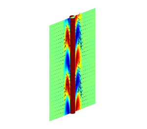
  $\kappa$, are both assumed to be independent of temperature and, as such, our analysis is restricted to temperature variations within the plume that are small relative to suitably chosen reference values. As illustrated in figure 1, the cylindrical coordinate system $\boldsymbol {r}=(r,\theta,z)$ is introduced where the $z$-axis is aligned with the axis of the cylinder, and the corresponding velocity components are $\boldsymbol {u}=(u,v,w)$. The surface of the cylinder and the ambient maintain vertical temperature distributions of $T_w(z)$ and $T_{\infty }(z)$, respectively.

Figure 1. Schematic of a vertical cylinder of radius  $r_0$ that extends infinitely in the $z$-direction, with surface temperature $T_w(z)$, in the gravitational field $(0,0,-g)$. The environment has temperature $T_{\infty }(z)$. The vertical velocity profile of the parallel base solution $W(r)$ is indicated together with the cylindrical coordinate system $(r,\theta,z)$.
While a cylinder of infinite extent is considered in this analysis, from a practical perspective the cylinder is assumed to be long enough to exclude the end effects and hence we restrict this stability study to self-similar laminar base flows which are expected to describe the flow far from either ends of the convection boundary layer or wall plume. The only possible temperature configurations which allow for similarity solutions are with both  $T_w(z)$ and $T_\infty (z)$ as linear functions (see Appendix A for a proof). Thus, we take
 \begin{equation} T_w(z)=N_w z+T_{w,0} \quad \text{and} \quad T_\infty(z)=N_\infty z+T_{\infty,0}, \end{equation}
where for a heated (as opposed to cooled) cylinder,  $T_w>T_{\infty }$ for all $z$ considered, and $T_{w,0}$ and $T_{\infty,0}$ are the (constant) temperatures of the wall and cylinder at $z=0$. The constants $N_w$ and $N_\infty$ are prescribed to be positive, indicating a stable stratification. We define a characteristic length scale $L$ for the environmental stratification as
 \begin{equation} L=(T_{w,0}-T_{\infty,0})/N_{\infty}. \end{equation}
Accordingly,  $L$ represents the change in elevation in the ambient over which the change in temperature is equal to the temperature difference at $z=0$ between the cylinder and ambient. For convenience, the buoyancy field $\phi =g\gamma (T-T_\infty )$, where $g$ and $\gamma$ denote the gravitational acceleration and coefficient of thermal expansion, respectively, is adopted as an alternative of the temperature field $T$ in the following formulation.
With the Grashof number defined as
 \begin{equation} Gr=(g\gamma(T_{w,0}-T_{\infty,0})L^3/\nu^2)^{1/4}, \end{equation}
following Jaluria & Gebhart (Reference Jaluria and Gebhart1974) and Tao et al. (Reference Tao, Le Quéré and Xin2004), the dimensionless variables are introduced as
 \begin{gather} \left. \begin{gathered}
\boldsymbol{r}=(L/Gr)\boldsymbol{r^*},\quad
\boldsymbol{u}=(\nu Gr^2/L)\boldsymbol{u^*},\quad
\phi=g\gamma(T_w-T_\infty)\phi^*,\quad t=\left(L^2/(\nu
Gr^3)\right)t^*,\\ p-p_\infty=(\rho\nu^2
Gr^4/L^2)p^*,\quad\psi=\mbox{(}\nu Gr
L\mbox{)}\psi^*, \end{gathered} \right\}
\end{gather}
\begin{gather} \left. \begin{gathered}
\boldsymbol{r}=(L/Gr)\boldsymbol{r^*},\quad
\boldsymbol{u}=(\nu Gr^2/L)\boldsymbol{u^*},\quad
\phi=g\gamma(T_w-T_\infty)\phi^*,\quad t=\left(L^2/(\nu
Gr^3)\right)t^*,\\ p-p_\infty=(\rho\nu^2
Gr^4/L^2)p^*,\quad\psi=\mbox{(}\nu Gr
L\mbox{)}\psi^*, \end{gathered} \right\}
\end{gather}
where the superscript  $(\boldsymbol {\cdot })^*$ indicates a dimensionless variable, $t$ is time, $\psi$ the Stokes streamfunction and $p_\infty =-\rho gz$ the hydrostatic pressure. The dimensionless radius of the cylinder is therefore $r_0^*=r_0Gr/L$. It is noteworthy that the buoyancy scale $g\gamma (T_w-T_\infty )$ may vary vertically, but all other scales and the Grashof number are independent of $z$. We take the experimental setting of Gladstone & Woods (Reference Gladstone and Woods2014) for an aqueous saline wall plume on a cylindrical buoyancy source as a reference for typical values of $Gr$ and $r_0^*$. From their figure 6(a) we estimate that $Gr\gtrsim 88$ and $r_0^*\approx 2.3$. Therefore, we take $Gr\sim {O}(100)$ and $r_0\sim {O}(1)$ as the reference values for the stability calculations that follow.
The cylindrical polar forms of the differential operators  $\boldsymbol {\nabla }$ and $\nabla ^2$ introduce additional complexities to the governing equations compared with the planar case considered by Tao et al. (Reference Tao, Le Quéré and Xin2004). Indeed, with the superscript $(\boldsymbol {\cdot })^*$ omitted hereafter, and defining the temperature gradient ratio $a$ and the Prandtl number as
 \begin{equation} a=N_w/N_{\infty} \quad \text{and} \quad Pr=\nu/\kappa, \end{equation}
the dimensionless conservation equations for mass, momentum and buoyancy are
 \begin{equation} \left. \begin{gathered} \boldsymbol{\nabla}\boldsymbol{\cdot}\boldsymbol{u}=0 ,\\ \displaystyle\frac{\mathrm{D}\boldsymbol{u}}{\mathrm{D}t}={-}\boldsymbol{\nabla} p+\frac{1}{Gr}\nabla^2\boldsymbol{u}+\frac{S(z)}{Gr}\phi\,\boldsymbol{e_z},\\ \displaystyle\frac{\mathrm{D}\phi}{\mathrm{D}t}=\frac{1}{PrGr}\nabla^2 \phi-\frac{1}{S(z)Gr} w\left(1+(a-1)\phi\right)+\frac{2(a-1)}{S(z)PrGr^2}\frac{\partial \phi}{\partial z}, \end{gathered} \right\} \end{equation}
respectively, where  $\boldsymbol {e_z}$ is the unit vector in the $z$-direction and
 \begin{equation} S(z)=1+(a-1)z/Gr \end{equation}
is the only coefficient in (2.6) that has a dependence on  $z$. As such, the degree of vertical inhomogeneity of the flow is characterised by the magnitude of $(a-1)/Gr$, which, if increased, leads to more rapid vertical variations of $S$. We consider only the cases with ${a \geq 0}$, which correspond to stable stratifications and heated cylinders. The respective boundary conditions on the cylindrical surface and in the environment are
 \begin{equation} \left.
\begin{aligned} \boldsymbol{u}=\boldsymbol{0},\quad
\phi=1, &\quad \mathrm{on} \ r=r_0, \\
\boldsymbol{u}=\boldsymbol{0},\quad \phi=0, &\quad \mathrm{as} \
r\to\infty. \end{aligned} \right\}
\end{equation}
\begin{equation} \left.
\begin{aligned} \boldsymbol{u}=\boldsymbol{0},\quad
\phi=1, &\quad \mathrm{on} \ r=r_0, \\
\boldsymbol{u}=\boldsymbol{0},\quad \phi=0, &\quad \mathrm{as} \
r\to\infty. \end{aligned} \right\}
\end{equation}
When the cylindrical wall and the environment have identical temperature gradients (i.e.  $N_w=N_\infty$), $S=a=1$ and, consequently, the system (2.6) can be reduced to a form that is independent of $z$. This special case is of considerable theoretical interest because, as pointed out in Tao et al. (Reference Tao, Le Quéré and Xin2004), the resulting parallel base buoyancy profile (which has no dependence on $z$) leads to a uniform flux of buoyancy from the wall. For general cases with $a\neq 1$, both the base flow and the stability characteristics vary vertically, a variation which is amplified at low Grashof numbers according to (2.7). Notably, the two limiting cases, $a\to 0$ and $a\to \infty$, correspond to an isothermal wall and an unstratified environment, respectively. While we set our focus on the uniform-buoyancy-flux case $a=1$, in what follows a few comments for $a \neq 1$ are also given in order to connect the results for $a=1$ to observations made in previous experiments in which the wall buoyancy flux usually deviated from being uniform.
3. Self-similar base flows
The boundary-layer approximation (Schlichting Reference Schlichting1960) is adopted to derive the steady axisymmetric laminar base flow. Accordingly, the dimensionless velocity components  $(U(r,z),0,W(r,z))$ and buoyancy $\varPhi (r,z)$ of the base flow satisfy
 \begin{gather} \left. \begin{gathered} W\displaystyle\frac{\partial W}{\partial z}+U\frac{\partial W}{\partial r}=\frac{1}{Gr}\frac{1}{r}\frac{\partial}{\partial r}\left(r\frac{\partial W}{\partial r}\right)+\frac{S(z)}{Gr}\varPhi,\\ W\displaystyle\frac{\partial \varPhi}{\partial z}+U\frac{\partial\varPhi}{\partial r}=\frac{1}{PrGr}\frac{1}{r}\frac{\partial }{\partial r}\left(r\frac{\partial \varPhi}{\partial r}\right)-\frac{1}{S(z)Gr}W\left(1+(a-1)\varPhi\right)+\frac{2(a-1)}{S(z)PrGr^2}\frac{\partial\varPhi}{\partial z}. \end{gathered} \right\} \end{gather}
A self-similar solution is sought of the form
 \begin{equation} \varPsi=S(z)f(\eta),\quad \varPhi=h(\eta),\quad\eta=r, \end{equation}
where  $\varPsi$ denotes the Stokes streamfunction for the base flow, and $f$,
$f$,  $h$ and $\eta$ are similarity variables. The velocity components are therefore
 \begin{equation} W=\frac{1}{r}\frac{\partial \varPsi}{\partial r}=S(z)\frac{f'}{\eta},\quad U={-}\frac{1}{r}\frac{\partial \varPsi}{\partial z}={-}\frac{a-1}{Gr}\frac{f}{\eta}, \end{equation}
where the prime  $(\boldsymbol {\cdot })'$ denotes differentiation once with respect to $\eta$. Evidently, the vertical velocity $W$ depends on both the radial and vertical coordinates but the radial velocity $U$ has no vertical dependence.
On substituting (3.2a–c) and (3.3a,b) into (3.1), the following coupled nonlinear ordinary differential equations (ODEs) are recovered:
 \begin{equation} \left. \begin{gathered} f'''+(a-1)ff''/\eta-f''/\eta-(a-1)f'^2/\eta-(a-1)ff'/\eta^2+f'/\eta^2+\eta h=0, \\ h''+(a-1)Pr\,fh'/\eta+h'/\eta-(a-1)Pr\,f'h/\eta-Pr\,f'/\eta=0, \end{gathered} \right\} \end{equation}
with the boundary conditions
 \begin{equation}
\left. \begin{aligned} f=f'=0,\quad h=1, &\quad \mathrm{on}\ \eta=\eta_0, \\ f'=h=0, &\quad
\mathrm{as}\ \eta\to\infty, \end{aligned} \right\}
\end{equation}
\begin{equation}
\left. \begin{aligned} f=f'=0,\quad h=1, &\quad \mathrm{on}\ \eta=\eta_0, \\ f'=h=0, &\quad
\mathrm{as}\ \eta\to\infty, \end{aligned} \right\}
\end{equation}
where  $\eta =\eta _0$ corresponds to the surface of the cylinder. On specifying $a$,
$a$,  $Pr$ and $r_0$, the above system of ODEs, as a boundary-value problem, is solved numerically. The algorithm consists of initially guessing the values of $f''$ and $h'$ at $\eta =\eta _0$, solving for the resulting profiles via the fourth-order Runge–Kutta method, updating the guesses by the Newton–Raphson method and looping until the profiles at large $\eta$ match the boundary conditions (3.5) at infinity.
3.1. Solutions for parallel base flows
For  $a=1$, the radial velocity vanishes and the vertical velocity depends only on $\eta$ (3.3a,b), indicating a purely vertically rising, i.e. a parallel, base flow. The cross-stream profiles of vertical velocity and buoyancy are plotted in figure 2 for various values of $r_0$ and $Pr$, values chosen purely for illustrative purposes. In the near-wall region, while the buoyancy ( $h$) declines with the radial coordinate ( $\eta$), the vertical velocity ( $f'/\eta$) increases and then decreases. At still greater radii, both the buoyancy and vertical velocity become negative before asymptoting to zero. These phenomena of ‘flow reversal’ and negative buoyancy are also common in the planar cases (Krizhevsky et al. Reference Krizhevsky, Cohen and Tanny1996; Tao et al. Reference Tao, Le Quéré and Xin2004), but notably, from figure 2(a,b) they become weaker for thinner cylinders. Indeed, for $r_0=0.01$ it is almost impossible to distinguish the flow reversal and negative buoyancy in the plots by eye. Meanwhile, as also shown in figure 2(a,b), a smaller cylinder radius always corresponds to an overall slower vertical flow with reduced shear and a sharper radial decrease of buoyancy. The plume thickness, characterised by the radial distance where either the vertical velocity or buoyancy approaches zero, appears to be relatively insensitive to the radius of the cylinder. Meanwhile, a higher Prandtl number, from figure 2(c,d), leads to a slower vertical flow, a sharper radial decrease of buoyancy and a thinner plume. These dependences on the Prandtl number are similar to those reported for a free axisymmetric plume (Chakravarthy et al. Reference Chakravarthy, Lesshafft and Huerre2015).

Figure 2. The self-similar base flow profiles when  $a=1$. (a,c) Vertical velocity profiles. (b,d) Buoyancy profiles. Panels show (a,b) $Pr=1$, (c,d) $\eta _0=1$.
Notably, compared with free plumes, the no-slip condition at  $r=r_0$ leads to fundamental changes to the base velocity and buoyancy profiles. Specifically, an inner sublayer forms within which the vertical velocity monotonically increases to its peak value with increasing radius, and the vertical velocity profile becomes much more diffusive. Defining the $1/e$-thickness as the radial distance from the cylinder surface at which the buoyancy or vertical velocity drops to $1/e$ of its maximum value, the ratio of buoyancy to velocity thicknesses, $\gamma$, can be considered as a characteristic quantity classifying such base profiles. When $Pr=1$, based on figure 2(a,b), we evaluate that this ratio is $\gamma \approx 0.25$ for a cylinder with radius $r_0=1$ and $\gamma$ decreases for thinner cylinders. By contrast, our evaluations based on figure 1 in Chakravarthy et al. (Reference Chakravarthy, Lesshafft and Huerre2015) suggest that $\gamma \approx 0.82$ at $Pr=1$ for free plumes. This drastic reduction in $\gamma$ due to the presence of a wall may suggest a qualitative change of the instability mechanism, e.g. from the Kelvin–Helmholtz to the Holmboe-like mechanisms, see Caulfield (Reference Caulfield2021).
3.2. Some comments on non-parallel base flows
According to (3.3a,b), when  ${a\neq 1}$ the base flow is two-dimensional and thus non-parallel. Moreover, depending on whether $a>1$ or $a<1$, the overall buoyancy forcing, represented by $(T_w-T_\infty )$, increases or decreases with $z$. Therefore, instead of showing cross-stream profiles, to gain insight we plot the two-dimensional streamlines (figure 3) for two representative non-parallel cases, $a=5$ and $a=0.2$, together with the parallel-flow reference case $a=1$. It should be borne in mind that the length and velocity scales can be very different between the two non-parallel cases because the characteristic length $L$ is a function of $a$, see (2.2) and (2.4).

Figure 3. The self-similar base streamline patterns for  $\eta _0=1$, $Pr=1$ and $Gr=100$ in two typical non-parallel cases, (a) $a=5$ and (b) $a=0.2$, and in the reference case of parallel flow (c) $a=1$. The plots show contours of constant $\varPsi$.
For  $a=5$ (figure 3a), fluid is drawn near horizontally towards the cylinder wall, the streamlines tilting slightly downwards (flow reversal), before rising in the region immediately adjacent to the cylinder wall. This flow pattern, representative of those predicted for general values of $a>1$, is thus characterised by a predominantly horizontal ‘induced flow’ field, i.e. entrainment, and a rising wall plume.
For  $a=0.2$ (figure 3b), the plume again rises vertically in the near-wall region but simultaneously fluid ‘peels off’ from the near-wall region, i.e. is detrained. Detrained fluid is drawn abruptly downwards before, with increasing $\eta$, titling upwards and flowing horizontally outwards into the environment. The reversal in flow direction that occurs beyond the immediate near-wall region is much stronger than the previous case of $a=5$, and is indicative of an ‘overturning’ motion. This flow pattern, representative of those predicted for general values of $a<1$, is of a detraining nature and thereby cannot be sustained at all heights. This assertion is consistent with the fact that, for $0 \leq a<1$, the temperature difference between the wall and environment reverses the sign at a sufficiently large height and thus the plume stops rising under buoyancy.
Although showing a laminar flow pattern, figure 3(b) is reminiscent of the peeling-plume model proposed in Bonnebaigt et al. (Reference Bonnebaigt, Caulfield and Linden2018) for a detraining turbulent wall plume in a stratified environment. If we admit a correspondence between the actual turbulent state and the laminar base flow, the turbulent flow can be regarded as being more likely to exhibit net entrainment or detrainment depending on whether  $a>1$ or $a<1$, respectively. This viewpoint is supported by some previous observations. Caudwell et al. (Reference Caudwell, Flór and Negretti2016) reported classic entrainment phenomena for wall plumes at the initial stages of the filling-box processes, i.e. when the ambient stratification is negligible (consistent with $a>1$), whereas significant detrainment was reported in Bonnebaigt et al. (Reference Bonnebaigt, Caulfield and Linden2018) for a filling box at large time when the environment would have been strongly stratified (consistent with $a<1$). Most convincingly, in the experiments of Gladstone & Woods (Reference Gladstone and Woods2014), where the entrainment and detrainment were reported to be of equal amount, their measurements indicated that the ratio of vertical buoyancy gradients between the plume and the ambient was near unity – a finding that corresponds to $a\approx 1$ if the vertical buoyancy gradient of the cylindrical surface can be approximated as that of the plume.
4. Stability analysis
With the tilde  $\tilde {(\boldsymbol {\cdot })}$ denoting the perturbation variables, on substituting $\boldsymbol {u}=\boldsymbol {U}+\boldsymbol {\tilde {u}}$, ${p=\tilde {p}}$ and $\phi =\varPhi +\tilde {\phi }$ into (2.6) and neglecting the products of perturbation quantities, the linearised equations for the perturbations are
 \begin{equation} \left. \begin{gathered} \boldsymbol{\nabla}\boldsymbol{\cdot}\boldsymbol{\tilde{u}}=0 ,\\ \displaystyle\frac{\partial\boldsymbol{\tilde{u}}}{\partial t}={-}\boldsymbol{U}\boldsymbol{\cdot}\boldsymbol{\nabla}\boldsymbol{\tilde{u}}-\boldsymbol{\tilde{u}}\boldsymbol{\cdot}\boldsymbol{\nabla}\boldsymbol{U}-\boldsymbol{\nabla} \tilde{p}+\frac{1}{Gr}\nabla^2\boldsymbol{\tilde{u}}+\frac{S}{Gr}\tilde{\phi}\,\boldsymbol{e_z},\\ \displaystyle\frac{\partial\tilde{\phi}}{\partial t}={-}\boldsymbol{U}\boldsymbol{\cdot}\boldsymbol{\nabla}\tilde{\phi}-\boldsymbol{\tilde{u}}\boldsymbol{\cdot}\boldsymbol{\nabla}\varPhi+\frac{1}{PrGr}\nabla^2\tilde{\phi}-\frac{1}{SGr} \tilde{w}-\frac{a-1}{SGr}(W\tilde{\phi}+\tilde{w}\varPhi)+\frac{2(a-1)}{SPr\,Gr^2}\frac{\partial\tilde{\phi}}{\partial z}, \end{gathered} \right\} \end{equation}
with boundary conditions
 \begin{equation} \left. \begin{aligned}
\tilde{u}=\tilde{v}=\tilde{w}=\tilde{p}=\tilde{\phi}=0, &\quad \mathrm{on} \ r=r_0, \\
\tilde{u}=\tilde{v}=\tilde{w}=\tilde{p}=\tilde{\phi}=0, &\quad \mathrm{as} \ r\to\infty. \end{aligned} \right\}
\end{equation}
\begin{equation} \left. \begin{aligned}
\tilde{u}=\tilde{v}=\tilde{w}=\tilde{p}=\tilde{\phi}=0, &\quad \mathrm{on} \ r=r_0, \\
\tilde{u}=\tilde{v}=\tilde{w}=\tilde{p}=\tilde{\phi}=0, &\quad \mathrm{as} \ r\to\infty. \end{aligned} \right\}
\end{equation}
It is noteworthy that the boundary condition for buoyancy adopted at the cylinder–fluid interface,  $\tilde {\phi }(r_0)=0$, can only be held in experiments for cylinders with sufficiently large thermal capacities. According to Knowles & Gebhart (Reference Knowles and Gebhart1968), this buoyancy condition needs to be modified for cylinders with small thermal capacities and will become the Neumann condition $\partial \tilde {\phi }/\partial r|_{r=r_0}=0$ when the cylinder is of zero thermal capacity, e.g. as in the case of a thin electrically heated wire.
Normal mode disturbances are now introduced in the form
 \begin{equation} (\tilde{u},\tilde{v},\tilde{w},\tilde{p},\tilde{\phi})=(\hat{u}(r),\hat{v}(r),\hat{w}(r),\hat{p}(r),\hat{\phi}(r)) \exp({{\rm i}(k z+n\theta-\omega t)})+\mathrm{c.c.}, \end{equation}
where, as is standard,  $\textrm {i}$ is the imaginary unit, c.c. refers to the complex conjugates, the integer $n$ denotes the azimuthal wavenumber, the axial wavenumber $k=k_r+\textrm {i}k_i$ and frequency $\omega =\omega _r+\textrm {i}\omega _i$ are generally complex and the hatted variables represent the radial structure of the disturbance. On substituting (4.3) into (4.1), the linear stability of the wall plume is governed by the following relations:
 \begin{gather} \left. \begin{gathered} r\displaystyle\frac{\mathrm{d} \hat{u}}{\mathrm{d} r}+\hat{u}+{\rm i}n\hat{v}+{\rm i}kr\hat{w}=0,\\ {\rm i}(k W-\omega)\hat{u}+U\displaystyle\frac{\mathrm{d}\hat{u}}{\mathrm{d} r}+\frac{\mathrm{d}U}{\mathrm{d}r}\hat{u}={-}\frac{\mathrm{d}\hat{p}}{\mathrm{d} r}+\frac{1}{Gr}\left[\frac{\mathrm{d}^2\hat{u}}{\mathrm{d} r^2}+\frac{1}{r}\frac{\mathrm{d}\hat{u}}{\mathrm{d} r}-\left(k ^2+\frac{n^2+1}{r^2}\right)\hat{u}-\frac{2{\rm i}n\hat{v}}{r^2}\right],\\ {\rm i}(kW-\omega)\hat{v}+U\displaystyle\frac{\mathrm{d}\hat{v}}{\mathrm{d} r}+\frac{U\hat{v}}{r}={-}\frac{{\rm i}n\hat{p}}{r}+\frac{1}{Gr}\left[\frac{\mathrm{d}^2\hat{v}}{\mathrm{d} r^2}+\frac{1}{r}\frac{\mathrm{d}\hat{v}}{\mathrm{d} r}-\left(k ^2+\frac{n^2+1}{r^2}\right)\hat{v}+\frac{2{\rm i}n\hat{u}}{r^2}\right],\\ {\rm i}(k W-\omega)\hat{w}+U\displaystyle\frac{\mathrm{d}\hat{w}}{\mathrm{d} r}+\frac{\partial W}{\partial r}\hat{u}+\frac{\partial W}{\partial z}\hat{w}={-}{\rm i}k \hat{p}+\frac{S}{Gr}\hat{\phi}+\frac{1}{Gr}\left[\frac{\mathrm{d}^2\hat{w}}{\mathrm{d} r^2}+\frac{1}{r}\frac{\mathrm{d}\hat{w}}{\mathrm{d} r}-\left(k ^2+\frac{n^2}{r^2}\right)\hat{w}\right],\\ {\rm i}(k W-\omega)\hat{\phi}+U\displaystyle\frac{\mathrm{d}\hat{\phi}}{\mathrm{d} r}+\frac{\mathrm{d}\varPhi}{\mathrm{d}r}\hat{u}=\displaystyle\frac{1}{PrGr}\left[\frac{\mathrm{d}^2\hat{\phi}}{\mathrm{d} r^2}+\frac{1}{r}\frac{\mathrm{d}\hat{\phi}}{\mathrm{d} r}-\left(k ^2+\frac{n^2}{r^2}\right)\hat{\phi}\right]-\frac{1+(a-1)\varPhi}{SGr}\hat{w}\\ +\displaystyle\frac{a-1}{SGr}\left(\frac{2{\rm i}k }{PrGr}-W\right)\hat{\phi}, \end{gathered} \right\} \end{gather}
where both  $S$ and $W$, as defined in (2.7) and (3.3a,b), have dependencies on $z$. From (4.2), the corresponding boundary conditions are
 \begin{equation} \left. \begin{aligned}
\hat{u}=\hat{v}=\hat{w}=\hat{p}=\hat{\phi}=0, &\quad \mathrm{on}
\ r=r_0, \\ \hat{u}=\hat{v}=\hat{w}=\hat{p}=\hat{\phi}=0, &\quad
\mathrm{as} \ r\to\infty. \end{aligned} \right\}
\end{equation}
\begin{equation} \left. \begin{aligned}
\hat{u}=\hat{v}=\hat{w}=\hat{p}=\hat{\phi}=0, &\quad \mathrm{on}
\ r=r_0, \\ \hat{u}=\hat{v}=\hat{w}=\hat{p}=\hat{\phi}=0, &\quad
\mathrm{as} \ r\to\infty. \end{aligned} \right\}
\end{equation}
When  $a=1$, $U=0$ and all $z$-dependences in (4.4) vanish, in which case the stability characteristics are invariant along $z$.
$z$.
Since a temporal stability analysis is more relevant for the current type of physical problem according to Huerre & Monkewitz (Reference Huerre and Monkewitz1990), we investigate the temporal branches of (4.4) with the axial wavenumber  $k$ being real. The system (4.4) subject to (4.5) is solved numerically as a general eigenvalue problem via the MATLAB subroutine ‘ $eig$’ on a radial domain $[r_0,r_0+r_m]$, where the constant $r_m\gg r_0$. This radial domain is mapped through $r-r_0=A(1+\xi )/(B-\xi )$, where $\xi$ is taken from the Chebyshev collocation points on the interval $[-1,1]$, $B=1+2A/r_m$ and $A$ is the radial distance from the cylinder surface within which half of the collocation points are located (Khorrami, Malik & Ash Reference Khorrami, Malik and Ash1989). The values of $A$ and $r_m$ are set appropriately to resolve sufficiently the perturbation profiles which can have rapid spatial variations near the cylinder surface. After some trial and error, we set $A=3$ and $r_m=12$, which leads to $B=1.5$; this choice of values always leads to convergence of the numerical scheme.
4.1. Dispersion relationships
The following analysis focuses on the uniform-buoyancy-flux case ( $a=1$) as this provides a useful reference for the general thermal configurations prescribed by $a\geq 0$.
Multiple numerical solutions exist for the eigenvalue problem (4.4) and, for a representative set of parameters, we plot in figure 4(a–d) the dispersion relationships  $\omega _i(k)$ of the eigenmodes with the five largest growth rates (at the wavenumber corresponding to the maximum $\omega _i$) for the azimuthal wavenumbers $n=0,1,2$ and $3$, respectively. It is evident that there are two types of eigenmode: the ‘type-A’ eigenmodes represented by cambered black curves with one or two peaks, and multiple ‘type-B’ eigenmodes that manifest as a cluster of quasi-straight lines which are generally decreasing functions of $k$. While for each azimuthal wavenumber the type-B eigenmodes are usually stable ( $\omega _i<0$), a single type-A eigenmode can be unstable ( $\omega _i>0$) on an interval of $k$ and dominate the perturbation growth, except for $n=3$; the type-B eigenmodes exhibit almost no significant changes with respect to the shapes and magnitudes of their $\omega _i(k)$-curves with varying $n$. For $n\geq 1$, the growth rate of that single type-A eigenmode decreases dramatically with $n$. Indeed, for $n=3$ the type-A eigenmode becomes so weak that its $\omega _i(k)$-curve is located well below those of the type-B eigenmodes and does not sit on the $k$–
$k$– $\omega _i$ domain of figure 4(d). It should be kept in mind that the trend in figure 4 about whether a given azimuthal mode is unstable or not, or which azimuthal mode is dominant, does not remain when the parameters change.

Figure 4. Dispersion relationships for the five leading eigenmodes on the temporal branch when  $a=r_0=Pr=1$ and $Gr=500$. Panels show (a) $n=0$, (b) $n=1$, (c) $n=2$, (d) $n=3$. The black curve denotes the $\alpha$-mode.
Nevertheless, based on the observations above and previous results for plumes of a cylindrical geometry (Wakitani Reference Wakitani1980; Riley & Tveitereid Reference Riley and Tveitereid1984; Chakravarthy et al. Reference Chakravarthy, Lesshafft and Huerre2015), hereafter, we can safely exclude the cases of  ${n\geq 2}$ in the remainder of the analysis because these higher azimuthal modes are always considerably more stable than the first helical mode ${(n=1)}$. Meanwhile, for both the axisymmetric ( ${n=0}$) and helical ( ${n=1}$) modes, only the outstanding type-A eigenmode needs to be taken into consideration. For true annular plumes, the perturbation modes may saturate at large time due to nonlinear effects and exhibit oscillatory motions. Whenever comparisons with experiments or numerical simulations are needed, the axisymmetric or helical modes in our linear stability analysis may be conveniently related, respectively, to the nonlinear ‘axisymmetric puffing’ or ‘rotating wave’ modes reported in Marques & Lopez (Reference Marques and Lopez2014) for a free round plume generated by a heated horizontal patch on the ground. However, in our case, the axisymmetric puffs of hot fluid into the ambient are anticipated to be horizontal (rather than vertical) due to the distinct configuration of our heat source.
The dependencies of the dispersion relationships on the Grashof number, dimensionless cylinder radius and Prandtl number are plotted in figure 5 based on computing the most unstable eigenmode of (4.4) for  $n=0$ and $1$. As shown in figure 5(a,b), the maximum growth rates, $\omega _{i,max}$, of both the axisymmetric and helical modes increase with $Gr$ – the wider band of unstable axial wavenumbers indicating an increasingly unstable flow. However, for $Gr\gtrsim 700$, the curves asymptote to a limiting curve and the maximum growth rate becomes independent of $Gr$. Notably, the helical mode consistently yields the higher maximum growth rate. A unique feature of the axisymmetric mode is that with $Gr$ decreasing, an additional peak of $\omega _i(k)$ at a lower axial wavenumber appears and may even dominate the perturbation growth, e.g. note the $Gr=300$ curve in figure 5(a). Such a long-wave peak can also exist for the helical mode at very low $Gr$ but its magnitude is trivial compared with the short-wave peak – see the $Gr=100$ curve in figure 5(b).

Figure 5. Dispersion relationships for the parallel case  $a=1$. The perturbation growth rate $\omega _i$ vs the real wavenumber $k$ for various (a,b) Grashof numbers, (c,d) dimensionless radii $r_0$ and (e, f) Prandtl numbers. Panels (a,c,e) (solid curves) show the axisymmetric mode $(n=0)$. Panels (b,d, f) (dot-dash curves) show the helical mode $(n=1)$. The reference values of the above parameters are $Gr=500$, $r_0=1$ and $Pr=1$. The $r_0=10^{-2}$ curve in (c) is not visible as it lies outside of the $k$–
$k$– $\omega _i$ domain shown.
From figure 5(c,d), thinner cylinders lead to more stable plume flows. With  $r_0$ decreasing, the maximum growth rate of the axisymmetric mode decreases significantly quicker than that of the helical mode. Therefore, for thin cylinders the helical mode dominates. For $r_0\gtrsim 10^2$, the $\omega _i(k)$-curves of both modes become identical and do not vary further with $r_0$. This result clearly lends confidence in the validity of the current algorithm for the stability calculations; this result is consistent with the fact that for sufficiently large $r_0$, the cylinder can be approximated as a planar wall – in which case, by the definition of normal modes (4.3), all azimuthal modes are identical irrespective of the value of $n$.
$n$.
According to figure 5(e, f), the maximum growth rate of either the axisymmetric or helical mode first decreases and then increases with  $Pr$, but this dependence is weaker for the axisymmetric mode. The critical value of $Pr$ corresponding to the minimal value of $\omega _{i,max}$ is different between the two azimuthal modes. The non-monotonic dependences may be due to the dual destabilising effects associated with shear and buoyancy. From the definition of the Prandtl number, and with reference to the base flow profiles in figure 2(c,d), while the destabilising effect of shear is prevalent at low $Pr$, the effect of buoyancy becomes strong at high $Pr$. Thus, the flow tends to be more unstable for both small and large $Pr$; both destabilising effects are not significant at intermediate $Pr$ so that the flow becomes relatively stable.
The maximum growth rates in these plots reveal that at large time (but still in the linear stage of instability), the exponentially growing perturbation can be either axisymmetric or helical for parameters in the normal range (by which we refer to the range not untypical for the complementary experimental works). This behaviour is quite different from that of a free axisymmetric plume or jet for which the helical mode is usually dominant at large time (Batchelor & Gill Reference Batchelor and Gill1962; Chakravarthy et al. Reference Chakravarthy, Lesshafft and Huerre2015).
4.2. Marginal instability behaviour
With either the cylinder radius or Prandtl number varying, (4.4) is solved over a domain in the  $k$–
$k$– $Gr$ space. The resulting neutral curves, consisting of contours representing zero growth rate, are plotted in figures 6 and 7 for the azimuthal wavenumbers $n=0$ and $1$. In general, each neutral curve can exhibit a single peak, or multiple peaks, where the threshold value of $Gr$ which will trigger instability when exceeded is at its minimum. The critical Grashof number $Gr_{cr}=\min \{Gr(k) \rvert _{\omega _i=0}\}$, is defined as the minimum Grashof number at which the flow can be marginally unstable, and visually corresponds to the peak protruding furthest to the left on each neutral curve as plotted. When multiple peaks are present, for the axisymmetric mode ( $n=0$) the critical Grashof number is always from the long-wave peak, but for the helical mode ( $n=1$) it is determined from the short-wave peak except when $Pr$ is sufficiently large – see figure 7(d) for such an exception. Evidently, the critical Grashof numbers of both modes can be of a similar order of magnitude, which means that when increasing $Gr$, the marginally unstable flow can exhibit either an axisymmetric or a helical perturbation, depending on $r_0$ and $Pr$.
$Pr$.

Figure 6. The neutral curves for the axisymmetric mode  $n=0$ (solid) and helical mode $n=1$ (dot-dashed) with $a=1$, $Pr=1$ and (a) $r_0=0.01$, (b) $r_0=0.1$, (c) $r_0=1$ and (d) $r_0=10$.

Figure 7. The neutral curves for the axisymmetric mode  $n=0$ (solid) and helical mode $n=1$ (dot-dashed) for $a=1$, $r_0=1$ and (a) $Pr=0.5$, (b) $Pr=1$, (c) $Pr=2$ and (d) $Pr=4$.
The dependencies of the marginal instability state on the dimensionless cylinder radius and Prandtl number are further illustrated in figure 8, which shows the critical Grashof number plotted as a function of  $r_0$ or $Pr$. The critical Grashof number of the axisymmetric mode decreases rapidly when the cylinder radius is increased, whereas the critical Grashof number of the helical mode has, by comparison, a weak dependence on $r_0$, see figure 8(a). For $r_0\lesssim 2.1$, the helical mode has a lower critical Grashof number. Thus, for thin cylinders (i.e. $r_0\lesssim 2.1$), when increasing the Grashof number, e.g. by enhancing the temperature difference between the cylinder and the ambient, the first unstable perturbation mode to be triggered is always helical. The difference in the critical Grashof number between the two azimuthal modes decreases with $r_0$ and for $r_0\gtrsim 2.1$, the axisymmetric mode becomes the most unstable, although its critical Grashof number is close to that of the helical mode. The critical Grashof numbers of both modes asymptotically approach an identical constant when the radius of the cylinder is sufficiently large (a constant we evaluate to be 56 at $Pr=1$), our predictions indicating that the cylindrical surface can be approximated as a planar wall for $r_0 \gtrsim 30$, see figure 8(a).

Figure 8. The variations of the critical Grashof number for the axisymmetric mode  $n=0$ (solid) and helical mode $n=1$ (dot-dashed) for the parallel case $a=1$ with (a) the dimensionless cylinder radius for $Pr=1$ and (b) the Prandtl number for $r_0=1$.
Figure 8(b) suggests that on increasing the Prandtl number the critical Grashof numbers of both the axisymmetric and helical modes first increase and then decrease. The helical mode is triggered at a lower  $Gr_{cr}$ when $Pr\lesssim 1.5$ but the axisymmetric mode is triggered when $Pr\gtrsim 1.5$. These individual dependencies are not strong enough to neglect the contribution of one or the other azimuthal mode to the instability when changing $Pr$. Notably, these features are distinct from those of a free axisymmetric plume where the helical mode almost always dominates the marginal instability (Chakravarthy et al. Reference Chakravarthy, Lesshafft and Huerre2015).
5. Destabilising mechanisms
5.1. Perturbation patterns
Based on the solutions of (4.4), the streamline pattern and buoyancy distribution are now examined for the most unstable mode of perturbation. A Grashof number of  ${Gr=500}$ is chosen for this analysis because, with reference to figure 5(a), the corresponding dispersion relationship with $n=0$ has two outstanding peaks of similar magnitudes (the short-wave peak is slightly higher). While each peak may arise due to a given destabilising mechanism, the long-wave ( $k\approx 0.22$) and short-wave ( $k\approx 0.41$) modes are investigated separately at this Grashof number in order to gain a more complete view of the phenomenology associated with the growth of perturbations.
The streamline patterns and buoyancy fields for the long-wave and the short-wave axisymmetric perturbation modes are shown in figures 9(a) and 9(b), respectively. Since an axisymmetric perturbation is invariant with the azimuthal angle  $\theta$, these flow patterns are plotted only on a single vertical cross-section at $\theta =0$. These flow patterns consist of a vertical array, or stack, of counter-rotating cellular toroidal-like structures, or convection cells, aligned along the surface of the cylinder. With $r$ increasing, we may infer from the streamline separation that the magnitude of the perturbation velocity increases relatively rapidly from zero and then decreases more gradually within these cells. Pronounced circulatory motions are sustained for $r \lesssim 10$ (figure 9), which is well beyond the radius for which the base vertical velocity is non-trivial ( $r\lesssim 5$, figure 2a). This indicates that organised, structured perturbation flows are significant in regions of the ambient which were quiescent in the unperturbed base state. For the larger of the two axial wavenumbers, the centre of a cell is located marginally closer to the cylinder wall and the lower-left region of the cell displays a more pronounced overturning motion (discussed further below). Meanwhile, the regions of positive and negative perturbation buoyancy (coloured red and blue, respectively) alternate vertically and are confined within arrowhead-shaped regions (hereinafter a ‘unit’) located adjacent to the wall. For both modes, the perturbation buoyancy is intensified in the near-surface region (here for $r\lesssim 3.5$) which corresponds approximately to the same radial range over which the base buoyancy is significant (figure 2b). On comparing the streamline patterns and buoyancy distributions, it is apparent that the streamlines are relatively closely spaced in the lower-right part of each buoyancy unit and sparse in the remaining part. Concerning the mixing process, it is evident that plume fluid from a region of positive perturbation buoyancy is always drawn outwards (outflow) into the ambient and then circulates back into the region of negative perturbation buoyancy near the surface. Thereafter, the fluid in a negative buoyancy region flows quasi-vertically into the nearby positive buoyancy region to compensate for fluid loss from the latter due to the buoyant outflow. Thus, this pattern of perturbation serves to mix positive perturbation buoyancy from the plume downwards in one cell, upwards in the next and so on.

Figure 9. The most unstable axisymmetric modes of perturbation for  $a=Pr=1$ and $Gr=500$ at the (a) long-wave peak ( $k=0.22$) and (b) short-wave peak ( $k=0.41$). Colour indicates the ratio of the buoyancy perturbation to its maximum, $\tilde {\phi }/\tilde {\phi }_{max}$. Red signifies a region of positive buoyancy perturbation and blue a region of negative buoyancy perturbation. The solid lines with arrows are the perturbation streamlines. The cylinder (left), with $r_0=1$, is shown as a shaded rectangle.
The  $n=1$ helical mode has a three-dimensional (3-D) flow pattern as is illustrated on both the azimuthal and horizontal cross-sections in figure 10; the pattern is shown for ${k=0.33}$, which corresponds to the single peak of its dispersion relationship (figure 5b). While all perturbation quantities vary as $\cos (\theta )$ azimuthally, on the azimuthal cross-section the perturbation buoyancy is distributed similarly to that of the axisymmetric mode with the arrowhead pattern again clearly evident. In the 3-D space, the buoyancy distribution exhibits a double-helix pattern which surrounds the cylinder and consists of a helix of fluid with positive perturbation buoyancy and another with negative perturbation buoyancy. Interestingly, in the perturbation flow field, most of the fluid motions are restricted within this double-helix structure. The fluid spirals upwards along the helix of positive buoyancy, and spirals downwards along the helix of negative buoyancy.

Figure 10. The most unstable helical mode for  $a=r_0=Pr=1$, $Gr=500$ and $k=0.33$. The colour scale indicates the ratio of the buoyancy perturbation to its maximum and the arrows represent the velocity vectors. The cross-sectional views are shown at (a) $\theta =0$ (right) and ${\rm \pi}$ (left), and (b) $z=-10$, $0$ and $10$. Red signifies a region of positive buoyancy perturbation and blue a region of negative buoyancy perturbation.
For both azimuthal modes, it is noteworthy that immediately adjacent to the cylinder surface (e.g.  $r-r_0\lesssim 1$ in the case of figure 9a), the slow-moving fluid can exhibit a reversal of vertical flow direction. Most evident in the axisymmetric case, this behaviour leads to a remarkable feature in the lower-left region of each convection cell, namely, a pronounced overturning motion in which the flow direction turns by 180 degrees (approximately). Referred to as the inner layer hereinafter, this narrow region is primarily due to the mean shear being positive in the near-wall region ( $\mathrm {d}W/\mathrm {d}r>0$), whereas in the significantly wider outer layer, the mean shear is negative (see figure 2). Compared with the flow outside, the different sign of shear in the inner layer leads to opposite vertical forcing and therefore abnormal flow directions relative to a classic free plume (Chakravarthy et al. Reference Chakravarthy, Lesshafft and Huerre2015) during the instability process.
5.2. Energy considerations
To develop an understanding of the physical mechanisms behind the growth of perturbations associated with the annular plume flow of interest, it is informative to examine the energy and work related to the instability. Multiplying (2.6) by  $\boldsymbol {\tilde {u}}$, the (non-dimensional) perturbation kinetic energy balance for the uniform-buoyancy-flux case ( $a=1$) is derived as
 \begin{equation} \displaystyle\frac{\partial\left(|\boldsymbol{\tilde{u}}|^2/2\right)}{\partial t}=\boldsymbol{\nabla}\boldsymbol{\cdot}\left(-\frac{\boldsymbol{U}|\boldsymbol{\tilde{u}}|^2}{2}-\tilde{p}\boldsymbol{\tilde{u}}+\frac{1}{Gr}\boldsymbol{\tilde{u}}\times\boldsymbol{\tilde{\xi}}\right)-\tilde{w}\tilde{u}\frac{\mathrm{d} W}{\mathrm{d} r}+\frac{1}{Gr}\tilde{w}\tilde{\phi}, \end{equation}
where the perturbation vorticity  $\boldsymbol {\tilde {\xi }}=\boldsymbol {\nabla }\times \boldsymbol {\tilde {u}}$. For general thermal configurations ( $a\neq 1$), there will be two additional production terms in (5.1), and the buoyancy term will vary linearly with height. With the notation $\langle \boldsymbol {\cdot }\rangle$ defined such that $\langle \boldsymbol {\cdot }\rangle := \int _{r_0}^{\infty }r(\boldsymbol {\cdot })\,\mathrm {d}r$, integrating (5.1) over a horizontal cross-section and a vertical wavelength $[0,\lambda ]$ yields the total energy balance
 \begin{equation} 2\omega_i\mathcal{K}=\mathcal{P}+\mathcal{B}-\mathcal{D}, \end{equation}
where
 \begin{equation} \left. \begin{gathered} \mathcal{K}=\displaystyle\int_0^\lambda\langle K\rangle\,\mathrm{d}z, \quad \mathcal{P}=\int_0^\lambda\langle P\rangle\,\mathrm{d}z,\quad \mathcal{B}=\int_0^\lambda\langle B\rangle\,\mathrm{d}z,\quad \mathcal{D}=\int_0^\lambda\langle D\rangle\,\mathrm{d}z,\\ K=\displaystyle\frac{1}{2}(\tilde{u}^2+\tilde{v}^2+\tilde{w}^2),\quad P={-}\frac{\mathrm{d} W}{\mathrm{d} r}\tilde{u}\tilde{w},\quad B=\displaystyle\frac{1}{Gr}\tilde{w}\tilde{\phi}, \quad D=\displaystyle\frac{1}{Gr}|\boldsymbol{\tilde{\xi}}|^2. \end{gathered} \right\} \end{equation}
In (5.3), the quantities  $K$,
$K$,  $P$,
$P$,  $B$ and $D$ represent the kinetic energy, production of the mean shear, work done by the buoyancy force and viscous dissipation per unit mass, respectively. Following the process in Nachtsheim (Reference Nachtsheim1963), with the superscript $(\boldsymbol {\cdot })^{\dagger}$ denoting the complex conjugate, the corresponding total energy and work within one vertical wavelength for a normal mode perturbation is derived as
 \begin{gather} \left. \begin{gathered}
\mathcal{K}=\displaystyle\frac{1}{2}\langle\hat{u}\hat{u}^{\dagger}+\hat{v}\hat{v}^{\dagger}+\hat{w}\hat{w}^{\dagger}\rangle,\quad
\mathcal{P}={-}\displaystyle\frac{1}{2}\frac{\mathrm{d}
W}{\mathrm{d}
r}\langle\hat{u}\hat{w}^{\dagger}+\hat{u}^{\dagger}\hat{w}\rangle,\quad
\mathcal{B}=\displaystyle\frac{1}{2Gr}\langle\hat{w}\hat{\phi}^{\dagger}+\hat{w}^{\dagger}\hat{\phi}\rangle,\\
\mathcal{D}=\displaystyle\frac{1}{Gr}\left\langle\frac{n^2}{r^2}|\hat{w}|^2+k^2|\hat{v}|^2-\frac{nk}{r}(\hat{v}\hat{w}^{\dagger}+\hat{v}^{\dagger}\hat{w})+k^2|\hat{u}|^2\right.\\
+\displaystyle\left|\frac{\partial\hat{w}}{\partial
r}\right|^2-{\rm
i}k\left(\hat{u}\displaystyle\frac{\partial\hat{w}}{\partial
r}^{\dagger}-\hat{u}^{\dagger}
\frac{\partial\hat{w}}{\partial
r}\right)+\left|\frac{\partial\hat{v}}{\partial
r}\right|^2+\displaystyle\frac{1}{r^2}|\hat{v}|^2+\frac{n^2}{r^2}|\hat{u}|^2\\
\left.+\displaystyle\frac{1}{r}\left(\hat{v}\frac{\partial\hat{v}}{\partial
r}^{\dagger}+\hat{v}^{\dagger}\frac{\partial\hat{v}}{\partial
r}\right)-\frac{in}{r}\left(\hat{u}\frac{\partial\hat{v}}{\partial
r}^{\dagger}-\hat{u}^{\dagger}
\frac{\partial\hat{v}}{\partial r}\right)-\frac{{\rm
i}}{r^2}\left(\hat{u}\hat{v}^{\dagger}-\hat{u}^{\dagger}
\hat{v}\right)\right\rangle. \end{gathered}
\right\} \end{gather}
\begin{gather} \left. \begin{gathered}
\mathcal{K}=\displaystyle\frac{1}{2}\langle\hat{u}\hat{u}^{\dagger}+\hat{v}\hat{v}^{\dagger}+\hat{w}\hat{w}^{\dagger}\rangle,\quad
\mathcal{P}={-}\displaystyle\frac{1}{2}\frac{\mathrm{d}
W}{\mathrm{d}
r}\langle\hat{u}\hat{w}^{\dagger}+\hat{u}^{\dagger}\hat{w}\rangle,\quad
\mathcal{B}=\displaystyle\frac{1}{2Gr}\langle\hat{w}\hat{\phi}^{\dagger}+\hat{w}^{\dagger}\hat{\phi}\rangle,\\
\mathcal{D}=\displaystyle\frac{1}{Gr}\left\langle\frac{n^2}{r^2}|\hat{w}|^2+k^2|\hat{v}|^2-\frac{nk}{r}(\hat{v}\hat{w}^{\dagger}+\hat{v}^{\dagger}\hat{w})+k^2|\hat{u}|^2\right.\\
+\displaystyle\left|\frac{\partial\hat{w}}{\partial
r}\right|^2-{\rm
i}k\left(\hat{u}\displaystyle\frac{\partial\hat{w}}{\partial
r}^{\dagger}-\hat{u}^{\dagger}
\frac{\partial\hat{w}}{\partial
r}\right)+\left|\frac{\partial\hat{v}}{\partial
r}\right|^2+\displaystyle\frac{1}{r^2}|\hat{v}|^2+\frac{n^2}{r^2}|\hat{u}|^2\\
\left.+\displaystyle\frac{1}{r}\left(\hat{v}\frac{\partial\hat{v}}{\partial
r}^{\dagger}+\hat{v}^{\dagger}\frac{\partial\hat{v}}{\partial
r}\right)-\frac{in}{r}\left(\hat{u}\frac{\partial\hat{v}}{\partial
r}^{\dagger}-\hat{u}^{\dagger}
\frac{\partial\hat{v}}{\partial r}\right)-\frac{{\rm
i}}{r^2}\left(\hat{u}\hat{v}^{\dagger}-\hat{u}^{\dagger}
\hat{v}\right)\right\rangle. \end{gathered}
\right\} \end{gather}
The spatial distributions of  $P$ and $B$ are investigated first for a few representative eigenmodes so as to acquire knowledge on how shear and buoyancy cooperate to destabilise the flow. Figure 11 shows the distributions of shear production and buoyancy work for two axisymmetric eigenmodes which correspond to the two peaks of the curve of $Gr=500$ in figure 5(a). While both the work of shear and buoyancy have positive and negative regions which are close to the surface of the cylinder and alternate vertically, the positive regions dominate. Noting that the distributions of $P$ and $B$ are both scaled on $P_{max}$, the maximum shear production, it is evident that the shear work is significantly stronger than the buoyancy work in both cases considered. Since the shear and buoyancy work are almost ‘in phase’ with respect to their vertical variations, they act to assist each other during the destabilising process. Notably, the location of the centre (or maximum) of the shear or buoyancy work appears to be insensitive to changes in $k$. In comparison with the base flow profiles in figure 2, the centre of the shear work always lies at the inflectional point (at $r\approx 2.5$) of the base vertical velocity profile. The centre of buoyancy work is close in radius to that of the shear work and is approximately where the mean buoyancy becomes zero. With $k$ increasing, the regions of negative shear and positive buoyancy work both diminish with smaller magnitudes throughout the domain, implying that for short waves, the shear mechanism dominates the instability whereas the buoyancy mechanism becomes important for long waves.

Figure 11. Colour map showing the distributions of the normalised (a,c) shear production  $P/P_{max}$ and (b,d) buoyancy work $B/P_{max}$ for the most unstable axisymmetric mode when $a=r_0=Pr=1$ and $Gr=500$. Panels show (a,b) $k=0.22$, (c,d) $k=0.41$. The azimuthal cross-section at $\theta =0$ is depicted.
A striking feature in figure 11 of the distribution of  $P$ is the narrow vertical band of elongated cells, located between the cylinder wall and the main larger cell-like region of shear work. While the shear work within can be either positive or negative, this ‘buffer’ region corresponds to the inner layer identified in § 5.1, within which slow overturning motions were reported. Interestingly, the buffer region is only evident for the short-wave mode in figure 11(c,d) and the shear work is in phase with that in the main region – for the long-wave mode in figure 11(a,b), the corresponding shear work becomes non-distinguishable and the band of elongated cells indistinct.
For the helical mode depicted in figure 12, an interesting difference from the axisymmetric mode is that both the near-field and main regions of shear work are staggered vertically. The shear work of the main region has a difference of phase of  $2{\rm \pi} /3$ (approx.) from that of the near-field region. Also, the regions with negative shear work almost vanish, indicating a robust shear mechanism of destabilising with purely positive shear production.

Figure 12. Colour map showing the distributions of the normalised (a) shear production  $P/P_{max}$ and (b) buoyancy work $B/P_{max}$ for the most unstable helical mode when $a=r_0=Pr=1$, $Gr=500$ and $k=0.33$. The azimuthal section at $\theta =0$ is depicted.
The relative contributions of  $\mathcal {P}$ and $\mathcal {B}$ to the growth of the total kinetic energy reveal the roles of different mechanisms in the instability process and, thus, are of primary interest. The ratio of total work $|\mathcal {B}/\mathcal {P}|$ is plotted as a function of the axial wavenumber $k$ in figure 13 for various Grashof numbers. For the axisymmetric mode (figure 13a), $|\mathcal {B}/\mathcal {P}|$ is generally a decreasing function of $k$. While buoyancy does more work for the long-wave perturbation modes, for the short-wave perturbation modes, shear work is the larger. The critical axial wavenumber at which the buoyancy work and shear work are equal is ${O}(10^{-1})$. For the helical mode (figure 13b), the ratio of work first increases and then decreases with the axial wavenumber, and it is noteworthy that the peak is always below unity – clear evidence that shear is more important for the helical mode. Interestingly, the peak value of $|\mathcal {B}/\mathcal {P}|$ is insensitive to the Grashof number and always around $|\mathcal {B}/\mathcal {P}|=0.6$. For both modes, the role of an increasing Grashof number is mainly to shift the corresponding curves to the left, and specifically for the axisymmetric mode, to make the instability more shear dominated. When the axial wavenumber decreases to sufficiently small values ( $k\sim {O}(10^{-2})$), there appear weakly growing axisymmetric modes with negative shear production (see the dashed curves in figure 11a) and helical modes with negative buoyancy work (see the dotted curves in figure 11b).

Figure 13. The variation of the ratio between the magnitudes of buoyancy and shear work,  $|\mathcal {B}/\mathcal {P}|$, on the vertical wavenumber $k$ for various Grashof numbers when $a=r_0=Pr=1$. Only the parts of curves corresponding to positive growth rates are shown. The solid part of each curve is where both shear and buoyancy work are positive. At the dashed/dotted part, shear/buoyancy does negative work. Panels show (a) $n=0$, (b) $n=1$.
The ratio of total buoyancy and shear work has also been computed over a range of dimensionless cylinder radius from  $10^{-2}$ to $10^2$ for various Prandtl numbers, see figure 14. For each setting of parameters, only the most unstable $k$ is analysed – the rationale being that this value of $k$ results in the highest growth rate and thus provides a useful representation of a band of wave-like disturbance that may occur in practice. For both modes, this ratio generally decreases with the radius of the cylinder, and this dependency appears much stronger for the axisymmetric mode and at low $Pr$. When the radius is sufficiently small, there are weakly growing axisymmetric perturbation modes with negative shear production. These trends indicate that high curvature of a cylindrical surface has a strong effect on reducing the shear work. This is essentially achieved, with reference to figure 2, via a flatter profile of the base vertical velocity. It is noteworthy that at intermediate $r_0$, for the axisymmetric mode, there can be an abrupt jump of $|\mathcal {B}/\mathcal {P}|$ from a value slightly above unity to a value well below unity. This jump marks a switch of the most unstable $k$ from the long-wave peak to the short-wave peak in the corresponding dispersion relationship – further evidence that the buoyancy work and shear work manifest for long and short waves, respectively. However, this jump diminishes for high $Pr$ at which the dispersion relationship only exhibits a single peak. Meanwhile, the ratio of buoyancy and shear work increases with the Prandtl number, indicating that fluids with high $Pr$ are more likely to exhibit a buoyancy-dominated growth of perturbations.

Figure 14. The variation of the ratio between the magnitudes of buoyancy and shear work,  $|\mathcal {B}/\mathcal {P}|$, on the dimensionless radius of the cylinder $r_0$ for the most unstable vertical wavenumber for various Prandtl numbers when $a=1$ and $Gr=500$. Only the parts of curves corresponding to positive growth rates are shown. The solid part of each curve is where both shear and buoyancy work are positive. At the dashed part, shear does negative work. Panels show (a) $n=0$, (b) $n=1$.
5.3. Inflectional mode vs wall mode
From the above results on the perturbation patterns and energy, a picture of the inflectional perturbation mode, either axisymmetric or helical (figure 11c,d or figure 12a,b) can be drawn. In common with the free plume/jet instability, the growth of perturbation is strongly linked to the presence of an inflection point of the base vertical velocity profile, which here is driven by the buoyancy difference between the cylinder surface and environment. Around the inflection point, significant shear work is transported from the base flow to the perturbation flow to trigger and sustain the destabilising process. Therefore, any factor reducing the base shear rate (e.g. higher curvature of the surface) or the radial range with significant shear (e.g. with higher  $Pr$) can contribute to stabilising the flow. The buoyancy perturbation generally plays an assisting role during the growth of the inflectional mode. While significantly weaker than the shear work, the positive buoyancy work is distributed over a region that tends to overlap the main region of positive shear work. This is because the buoyancy perturbation is produced largely by the vertical advection of fluid due to the vertical perturbation velocity which is the largest around the centre of positive shear work. Therefore, together with the shear work, the buoyancy work is also transferred into the perturbation kinetic energy around the inflection point.
Since the inflectional mode is characterised by the dominance of shear over buoyancy work, i.e. high  $|\mathcal {B}/\mathcal {P}|$, according to figures 13 and 14, it is prevalent for cylinders with large $r_0$, small $Pr$ and short waves. From the perspective of temporal instability, a packet of inflectional modes with relatively short wavelengths manifests, centred around the short-wave peak of the corresponding dispersion relationship, see figure 5.
Another perturbation mode, referred to hereinafter as the wall mode (figure 11a,b), can arise due to the presence of the cylindrical wall for both azimuthal modes. This is because, while a free plume only exhibits a single peak in the dispersion relationship (Wakitani Reference Wakitani1980; Riley & Tveitereid Reference Riley and Tveitereid1984; Chakravarthy et al. Reference Chakravarthy, Lesshafft and Huerre2015), with a wall, an additional long-wave peak of the dispersion relationships (figure 5) becomes probable – this peak represents a packet of long-wave instability modes driven by a qualitatively different destabilising mechanism. Physically, the presence of a wall dampens the rising of the plume and leads to a lower shear rate in the plume outer layer (figure 2), yielding weaker shear production of perturbation kinetic energy. From figure 11(a), while the inner layer exhibits trivial shear production, a large region of negative shear production is present near the inflection point, resulting in low total shear production. Nevertheless, according to figure 11(b), the buoyancy work becomes significant for this new destabilising mechanism and, therefore, the appearance of the wall mode can be detected by high  $|\mathcal {B}/\mathcal {P}|$.
Based on figures 13 and 14, the buoyancy-dominated wall mode manifests for thin cylinders, high  $Pr$ and long waves. Wherever an abrupt jump of $|\mathcal {B}/\mathcal {P}|$ is present, there is a switch between the inflectional and wall modes. It is noteworthy that the wall mode is more likely to be axisymmetric than helical, because a sufficiently high $Pr$ is mandatory for a helical mode to achieve a high $|\mathcal {B}/\mathcal {P}|$, see figure 14(b).
Noting that the inflectional mechanism (inflectional mode) is generally more robust than the buoyancy mechanism (wall mode), the competition between the two azimuthal cases ( $n=0$ and $n=1$) can be accounted for based on the two destabilising mechanisms. Take the marginal stability results in figure 8 as an example. When $Pr=1$, for thin cylinders, the wall mode dominates for an axisymmetric disturbance, whereas for a helical disturbance, the more robust inflectional mode remains dominant due to this low $Pr$. Therefore, the helical disturbance becomes prevalent for thin cylinders, yielding a lower critical Grashof number. With the cylinder radius increasing, the inflectional mode dominates for both azimuthal numbers and the critical Grashof numbers for both azimuthal cases become close. For cylinders with very large $r_0$ (approaching a planar wall), geometrically an axisymmetric disturbance and a helical disturbance are approximately the same, and thus the critical Grashof numbers for both azimuthal numbers are almost identical. Similarly, for low $Pr$, the helical inflectional mode overwhelms the axisymmetric inflectional mode due to the significant negative shear production associated with the latter (figure 11c), and thus the helical disturbance has a much lower $Gr_{cr}$. When $Pr$ becomes high, for both azimuthal cases, the wall mode is dominant, but the helical disturbance is associated with a much weaker buoyancy production – this is because the azimuthal component of perturbation velocity does not contribute directly to the generation of perturbation buoyancy and, therefore, the buoyancy mechanism for a helical disturbance is generally weaker than for an axisymmetric disturbance. Thus, for sufficiently high $Pr$, an axisymmetric cellular convection pattern first manifests on increasing the Grashof number.
6. Absolute $/$convective instability

Whether confined by the presence of a vertical wall, or free to develop in unbounded environments, some plumes have been observed to exhibit periodic flow patterns. A standout example is the intermittent entrainment and detrainment created by a release of saline solution from a micro-porous vertical cylinder into aqueous saline stratified surroundings reported by Gladstone & Woods (Reference Gladstone and Woods2014). Such self-excited oscillatory behaviours can be attributed to the absolute instability (Monkewitz et al. Reference Monkewitz, Bechert, Barsikow and Lehmann1990; Hallberg et al. Reference Hallberg, Srinivasan, Gorse and Strykowski2007; Lesshafft, Huerre & Sagaut Reference Lesshafft, Huerre and Sagaut2007). We hypothesise that, for wall plumes exhibiting the absolute instability over a sufficiently wide range of streamwise locations, in the nonlinear regime a global mode, characterised by the periodic puffing of hot fluid from the wall plume into the ambient, is established. To achieve the global oscillatory state, a wall plume undergoes a supercritical Hopf bifurcation whose mechanism may be analogous to the closed-loop feedback reported for free plumes in Meunier & Nadal (Reference Meunier and Nadal2018). The oscillatory puffing can be either axisymmetric or swirling (but axisymmetric in a rotational frame), which was discussed in detail in the numerical study of Marques & Lopez (Reference Marques and Lopez2014) for free plumes. While in Marques & Lopez (Reference Marques and Lopez2014), the hot fluid puffs vertically from a horizontal heated patch on the ground, due to the distinct thermal configuration in the present study, i.e. a vertically distributed heat source, puffing is achieved horizontally instead. This puffing mechanism may manifest as filaments of buoyant fluid being ejected intermittently into the ambient from the wall plume, i.e. the plume detrainment phenomenon. Thus, we proceed by investigating the absolute/convective stability characteristics of a wall plume along a cylinder. Again, our focus is with the  $a=1$ buoyancy configuration.
Based on the Briggs–Bers criteria (Huerre & Monkewitz Reference Huerre and Monkewitz1990), a saddle point of the complex function  $\omega (k)$ in the $k_r$– $k_i$-plane corresponds to the ‘absolute’ perturbation mode observed in the stationary frame of reference. The absolute mode at the saddle point has the complex wavenumber $k_0$ and complex frequency $\omega _0$, and group velocity $v_g:= \partial \omega /\partial k|_{k=k_0}=0$. It is essential to check if a saddle point satisfies the ‘pinching condition’ (Briggs Reference Briggs1964, Chapter 2), namely, from a visual perspective, if it is formed by a pinching of two curves originating from the upper and lower halves of the complex wavenumber plane. Only by satisfying the pinching condition can a saddle point really contribute to the absolute/convective instability. The flow is referred to as absolutely unstable if $\mathrm {Im}\{\omega _0\}=\omega _{0,i}>0$, $\mathrm {Im}\{\boldsymbol {\cdot }\}$ understood to be the imaginary part. Our computation is restricted to the most physically relevant eigenmode, the type-A mode, which dominates at least on the temporal branch (figure 4). The global topology of the multi-valued numerical dispersion relationship $\omega (k)$ for the present type of natural convection problems is usually highly complex due to the dual destabilising mechanism from shear and buoyancy, which makes the computation of the absolute modes challenging. What makes the situation even more problematic here is that for a wavenumber that is far away from the real $k$-axis, the type-A mode we are interested in can be weaker than the type-B modes, and these two types of modes cannot be distinguished simply by their complex frequencies. This limits the effectiveness of a traditional Newton-type iteration method for searching for the saddle point since it is difficult to identify the type-A eigenmode after every iteration. Suslov (Reference Suslov2006) proposed an iterative scheme for sorting the eigenvalues at each complex $k$ by means of a ‘shifted growth rate’, which, however, according to our computations, does not perform well when the saddle point is far away from the real-axis, as is the case in the present problem.
To tackle the difficulty of tracking the most temporally unstable mode over the complex  $k$-plane, we innovated an algorithm based on an initial value approach documented in Appendix B. The algorithm starts from an initial wavenumber $k_1$ at which the eigenvector and eigenvalue, $(\boldsymbol {q_1},\omega _1)$, of the eigenmode that we are interested in are both known. For example, for a moderate real $k_1$, the most temporally unstable eigenmode is almost always the one with the largest imaginary part $\omega _i$. Then, we solve the initial value problem derived by differentiating the eigenvalue system (4.4) from the initial wavenumber $k_1$ to a neighbouring wavenumber $k_2$ (Appendix B), which generates a prediction $(\boldsymbol {q'_2},\omega '_2)$ of this eigenmode at $k_2$. Next, we compute the multiple eigenmodes at $k_2$ by solving (4.4) in the normal way, and among the results, we identify and select the eigenmode, $(\boldsymbol {q_2},\omega _2)$, whose eigenvalue and eigenvector are the closet to the prediction $(\boldsymbol {q'_2},\omega '_2)$. By taking $k_2$ as the new initial wavenumber, the above process is repeated to acquire the global map of $\omega (k)$ for the eigenmode that we are interested in over the whole $k$-plane.
With the method above, the typical topology of the contours of  $\omega _{i}(k)$ is readily computed. Topologies so computed are shown in figure 15 for a representative setting of parameters for both the axisymmetric and helical modes. The lower-left corner of the $k$-plane is not displayed because we found that an extremely high resolution is required to resolve the contours in this corner. For a broad range of parameters, two saddles points, denoted as $S_1$ and $S_2$, are always detected, both satisfying the pinching condition. The upper-left saddle point $S_1$ always lies at an elevation higher than the lower saddle point $S_2$. Therefore, the absolute/convective instability is essentially determined by $S_1$. Since the growth rate at $S_1$, $\omega _{0,i}$, which we refer to as the absolute growth rate, is always negative, no absolute instability has been detected by us. For either azimuthal number $n=0$ or $n=1$, the absolute mode at $S_1$ exhibits a wavenumber whose real part is smaller than that of the most temporally unstable mode (i.e. an axially longer wave), but of the same order of magnitude ${O}(10^{-1})$, see figure 5(a,b) for comparison. Interestingly, for the axisymmetric mode, the two saddle points are located on an almost flat plateau whose elevation is within a narrow range from $-0.028$ to $-0.024$, in a broad domain of $k$. By contrast, the two saddle points for the helical mode are well separated with distinct elevations. We hereby propose that the upper-left and lower-right saddle points represent the inflectional and wall modes observed in the stationary frame, respectively. For the helical mode, $S_1$ has a much higher altitude and is much closer to the real axis than $S_2$, indicating that $S_1$ connects to the single (inflectional) peak of the temporal branch. Similarly, for the axisymmetric mode, both saddle points lie in close proximity with similar altitudes, which corresponds to the (inflectional and wall) double-peak structure of the temporal branch, see figure 5(a,b).

Figure 15. The global topology of  $\omega _i(k)$ for the most temporally unstable eigenmode when $a=r_0=Pr=1$ and $Gr=700$. The step between contours is $\Delta \omega _i=0.004$ and the saddle points, $S_1$ and $S_2$, are marked as solid circles. The neutral contours of $\omega _i=0$ are highlighted by thick black curves. (a) The axisymmetric mode $n=0$. (b) The helical mode $n=1$.
Although the absolute modes for the present thermal configuration  $(a=1)$ are always convectively unstable, it is still of interest to establish the dependency of the absolute growth rate on the cylinder radius. (We only focus on the upper-left saddle point $S_1$ since its absolute growth rate is always the larger.) Computing the global maps of $\omega _i$ for a wide range of $r_0$ is computationally demanding, and therefore we combine the initial value approach above with the Newton method to iteratively find the saddle point. The details of the algorithm and the improvements innovated by us are outlined in Appendix C.
The dependence of the absolute growth rate  $\omega _{0,i}$ at $S_1$ on the cylinder radius for various Grashof numbers when $Pr=1$ is shown in figure 16. For either the axisymmetric or helical mode, it is found that the absolute growth rate is negative, first decreasing and then increasing with increasing cylinder radius. Denoting the radius when the flow is the most absolutely stable as the critical radius $r_{0,c}$, we find $r_{0,c}\sim {O}(10^{-1})$ for the axisymmetric mode and $r_{0,c}$ for the helical mode. Additionally, we may assert that plumes along a planar wall, i.e. $r_0\to \infty$, are usually more absolutely unstable than plumes along cylinders, with exception of a helical mode developed on a sufficiently thin cylinder ( $r_0\sim {O}(10^{-2})$) when the Grashof number is large enough, see the dashed curve in figure 16(b). In other words, when $r_0$ is small enough, plumes along thinner cylinders are more susceptible to developing the absolute instability, global oscillatory patterns and therefore robust heat transfer – this trend is consistent with the experimental results of Popiel (Reference Popiel2008). The dependence of the absolute growth rate on the Grashof number is quite weak for thin cylinders. When the radius is large enough, e.g. $r_0>10$, the absolute growth rate becomes a decreasing function of $Gr$ for the axisymmetric mode, but first increases and then decreases with $Gr$ for the helical mode. These findings indicate that for increasingly large Grashof numbers (e.g. as achieved with stronger heating), the increasingly rapid rise of the plume due to the enhanced buoyancy forcing makes it increasingly difficult for a disturbance to spread upwards and downwards simultaneously to sustain the absolute instability. In addition, we plot the dependence of the absolute growth rate at $S_1$ on the Prandtl number for various Grashof numbers when $r_0=1$ in figure 17. For either azimuthal perturbation mode, the absolute growth rate is always negative and appears to be a generally increasing function of $Pr$ – the same trends were found in Tao et al. (Reference Tao, Le Quéré and Xin2004) for a planar wall plume with the thermal configuration $a=1$.

Figure 16. Absolute growth rate vs cylinder radius for various Grashof numbers when (a)  $n=0$ and (b) $n=1$. $a=Pr=1$.

Figure 17. Absolute growth rate vs Prandtl number for various Grashof numbers when (a)  $n=0$ and (b) $n=1$. $a=r_0=1$.
7. Conclusions
The linear instability of a wall plume generated on a vertical non-uniformly heated cylinder in a stratified environment has been explored with a special focus on the role of cylinder radius in the growth of perturbations. Our overriding motivation in addressing this fundamental problem was to gain insight into the mechanisms responsible for the intermittent patterns of entrainment and detrainment observed in experiments with vertically distributed buoyancy sources and to establish conditions for the onset of natural cellular convection from a laminar diffusive flow regime.
The laminar base flow was acquired by assuming self-similarity of the cross-stream profiles of vertical velocity and temperature, based on which the evolution of an infinitesimal perturbation of the classic Fourier form was analysed. The temporal instability problem, being cast in the form of an eigenvalue problem seeking normal mode solutions, was solved numerically with the Chebyshev collocation spectral method, and the absolute/convective instability problem investigated by searching for the saddle point(s) of the corresponding numerical dispersion relationship. While the theoretical framework we have developed is applicable for general thermal configurations with linear temperature gradients of the cylinder surface and environment, only the results for the uniform-buoyancy-flux case where the temperature gradients imposed on the cylinder and in the environment are identical, are presented and analysed. It is this, the  $a=1$ case, that forms the basis for the following conclusions.
Some general features of the type of instability identified are particularly noteworthy. Only the axisymmetric ( $n=0$) and the helical ( $n=1$) modes are of practical importance as the modes with higher azimuthal wavenumbers ( $n>1$) are all significantly weaker. Depending on the thermal conditions/wall curvature/fluid properties, as captured by $\{a, r_0, Pr, Gr\}$, either the axisymmetric or helical mode can be the more unstable under normal conditions. The flow pattern of an axisymmetric mode of perturbation is one of counter-rotating toroidal cells aligned vertically, whereas for the helical mode, the convection patterns are such that fluid spirals upwards and downwards simultaneously, forming a double-helix structure. Notably, for both azimuthal modes, there is one main region (centred at the inflection point) and one narrow near-field region of intensified shear work, the latter diminishing for long-wave perturbation modes. While the region of intensified buoyancy work overlaps to a large extent with the main region of shear work, the buoyancy work has a much stronger impact on destabilising the axisymmetric mode than the helical mode.
Increasing the temperature difference between the cylinder surface and environment, characterised by increasing the Grashof number, always leads to a more temporally unstable flow, but the growth rate of perturbation asymptotes to an upper bound. The minimum forcing, or temperature difference, required for the onset of convection, characterised by the critical Grashof number, depends on both the cylinder radius and Prandtl number as discussed below.
For thin cylinders ( $r_0\lesssim 2.1$ for $Pr=1$), when increasing $Gr$, the onset of thermal convection always manifests as triggering of a helical wave (e.g. double-helix structure). This is because, while in the planar limiting case both azimuthal modes are physically identical with a critical Grashof number of ${O}(10)$ (e.g. $Gr_{cr}\approx 56$ for $Pr=1$), with the cylinder radius decreasing, the critical Grashof number increases drastically for the axisymmetric mode but stays ${O}(10)$ for the helical mode. For cylinders of larger radii ( $r_0\gtrsim 2.1$ for $Pr=1$), although the axisymmetric mode is more unstable, both modes may be triggered together in practice since their critical Grashof numbers are remarkably close. Our energy analysis reveals that, below certain $r_0$, for moderate $Pr$, while the axisymmetric disturbance exhibits the wall mode, the more robust inflectional mode dominates the growth of the helical disturbance, which explains why the helical mode dominates at the onset of thermal convection on thin cylinders.
The Prandtl number is another crucial parameter determining the onset of thermal convection. While below the critical Prandtl number ( $Pr_{cr}\approx 1.5$ for $r_0=1$), the thermal convection is triggered as a helical wave-like motion, above the critical Prandtl number, an axisymmetric convective pattern manifests. Actually, either the axisymmetric or helical mode first becomes increasingly less unstable and then increasingly unstable with an increasing Prandtl number – a trend similar to that reported previously for the 2-D mode in the planar case (Krizhevsky et al. Reference Krizhevsky, Cohen and Tanny1996). However, unique to the cylindrical case here is that two azimuthal modes with totally different convective patterns dominate at different ranges of $Pr$.
$Pr$.
Some implications of the results for predicting the occurrence of detrainment are discussed based on the hypothesis made by us that the simultaneous entrainment and detrainment, and the pure entrainment phenomena, originate from the absolute and convective instabilities, respectively. Since the simultaneous entrainment and detrainment behaviour of plumes has been observed to manifest as oscillatory structures with intermittency at fixed heights (Gladstone & Woods Reference Gladstone and Woods2014; Bonnebaigt et al. Reference Bonnebaigt, Caulfield and Linden2018), such plumes are categorised by us into the oscillator type of flows which originate from the absolute instability (Huerre & Monkewitz Reference Huerre and Monkewitz1990). Meanwhile, since the classic entraining behaviour of plumes is always synonymous with engulfing eddies which develop and advect quickly with the mainstream, these plumes are regarded as the amplifier type and correspond to the convective instability. Therefore, the wall plumes considered by us with identical temperature gradients to the environment, being always convectively unstable, should only exhibit entrainment after the flow transition. This is because, for the current temperature configuration (weak ambient stratification), a growing wave packet, when advected upwards by the rising plume, undergoes insufficient negative buoyancy which aids it in spreading downwards simultaneously. Actually, the theoretical results of Tao et al. (Reference Tao, Le Quéré and Xin2004) for a heated planar wall also show that the absolute instability is only possible with a sufficiently strong ambient stratification.
We hereby assert that a strong stratification is an essential condition for the flow to be absolutely unstable and a prerequisite for detrainment. This assertion is also supported by our calculations of the base flow patterns for general temperature configurations. When the temperature gradient of the ambient exceeds that of the cylinder surface, the base flow exhibits a detrainment or ‘peeling-off’ pattern. If regarded as a summation of the base and perturbation flows, an actual plume should be more likely to detrain with a stronger background stratification. This condition of dominant ambient stratification was achieved in the experiments of Gladstone & Woods (Reference Gladstone and Woods2014) and Bonnebaigt et al. (Reference Bonnebaigt, Caulfield and Linden2018) due to the filling-box effect, and they both observed occurrences of detrainment.
From our calculations, the cylinder radius may have a significant effect on the occurrence of detrainment by affecting the absolute instability. When the cylinder becomes thinner, detrainment is first suppressed and then promoted. Plumes on ‘ultra-thin’ cylinders ( $r_0\lesssim 10^{-2}$ when $Pr=1$) can be more susceptible to establishing simultaneous entrainment and detrainment flow patterns than those on planar walls. By contrast, modifying the Grashof number, e.g. increasing the temperature difference between the cylinder surface and environment, only has minor effects on altering the turbulent structures.
Finally, it is worth mentioning that with the molecular diffusion neglected, a solely entraining plume can only transport the heat from the cylinder into the local environment via what may be regarded as the ‘filling-box’ effect, i.e. on forming a (displacement) horizontal intrusion about the height of neutral buoyancy; if confined by sidewalls, this heated fluid may be turned downwards, thereby penetrating heat further into the environment. By contrast, a plume that entrains and simultaneously detrains would appear to offer a more efficient means of transferring heat into the environment. Since the absolute instability is proposed by us to lead to the detrainment behaviour of the actual flows, knowledge of the onset of the absolute stability illuminates us in how to establish and sustain an engineering system with the preferable mixing mechanism, either of the pure entrainment or the entrainment-and-detrainment type. Take the thermal convection around a heated cylinder in an unbounded environment as an example. Simultaneous entrainment and detrainment should be a more efficient way of heat transfer than pure entrainment for the reasons discussed above. Therefore, based on our results, either using a thick ( $r_0\gtrsim {O}(10)$ when $Pr=1$) or ultra-thin ( $r_0\lesssim {O}(10^{-2})$ when $Pr=1$) cylinder can benefit establishing the flow pattern of simultaneous plume entrainment and detrainment, and promote the heat transfer. Alternatively, this preferred flow regime can be achieved by acquiring a small temperature gradient ratio $a$, e.g. heating the cylindrical surface more evenly or locating the cylinder in an environment that exhibits a relatively strong (stable) thermal stratification.
Declaration of interests
The authors report no conflict of interest.
Appendix A. Possible thermal configurations that allow for similarity solutions of a steady laminar annular wall plume in a stratified environment
Consider a cylindrical surface at  $r=R$ extending vertically along $z$ in a uniform medium of incompressible fluid of constant viscosity $\nu$ and thermal diffusivity $\kappa$. (The physical quantities considered hereinafter are all with dimensions.) The surface and ambient temperatures are maintained at $T_w(z)$ and $T_\infty (z)$, respectively, and without loss of generality we take $T_w(z)>T_\infty (z)$. This temperature differential generates a laminar axisymmetric flow with an upward axial velocity component $w$ and a radial velocity component $u$. Defining $T_0$ as the reference temperature, we define $c(z)$ and $d(z)$ such that
 \begin{equation} c(z)=T_\infty(z)-T_0,\quad d(z)=T_w(z)-T_\infty(z). \end{equation}
Neglecting the viscous dissipation and pressure work, under the Boussinesq and boundary layer approximations, the steady flow of an axisymmetric convection layer along the cylindrical surface is governed by (see Gebhart Reference Gebhart1971)
 \begin{equation} \left. \begin{gathered} \displaystyle\frac{\partial ru}{\partial r}+\frac{\partial rw}{\partial z}=0, \\ u\displaystyle\frac{\partial w}{\partial r}+w\frac{\partial w}{\partial z}=\nu\left(\frac{\partial^2 w}{\partial r^2}+\frac{1}{r}\frac{\partial w}{\partial r}\right)+g\beta\theta, \\ u\displaystyle\frac{\partial\theta}{\partial r}+w\frac{\partial\theta}{\partial z}=\kappa\left(\frac{\partial^2\theta}{\partial r^2}+\frac{1}{r}\frac{\partial\theta}{\partial r}\right)-w\frac{\mathrm{d} c}{\mathrm{d} z}, \end{gathered} \right\} \end{equation}
where  $\theta (z)=T(z)-T_\infty$ is the temperature excess relative to the ambient (or buoyancy) and $\beta$ the coefficient of thermal expansion. The dimensionless similarity variables are written as
 \begin{equation} f(\eta)=\frac{\psi}{\nu b(z)},\quad \phi(\eta)=\frac{\theta}{d(z)},\quad\eta=\frac{r}{a(z)}, \end{equation}
where  $\psi$ is the streamfunction defined, as is standard, such that $w=\partial \psi /(r\partial r)$ and $u=-\partial \psi /(r\partial z)$. The quantities $a(z)$, $\nu b(z)$ and $d(z)$ are the local scales of length, streamfunction and relative temperature, respectively.
The question arising now is for which ambient and wall temperature distributions,  $c(z)$ and $d(z)$, are there similarity solutions, namely, functions $a(z)$ and $b(z)$ which guarantee that $f$ and $\phi$ depend solely on $\eta$?
Substituting (A3a–c) into (A2) yields
 \begin{gather} \left. \begin{gathered} f'''-2a^2\eta f''+a^2 b_z\eta ff''+2a^2f'+(2aa_zb-a^2b_z)\eta f'^2-a^2b_zff'+\displaystyle\frac{g\beta a^6d}{\nu^2b}\eta^3\phi=0,\\ \displaystyle\frac{1}{Pr}\phi''+b_z\eta^{{-}1}f\phi'+\frac{1}{Pr}\eta^{{-}1}\phi'-\frac{bd_z}{d}\eta^{{-}1}f'\phi-\frac{bc_z}{d}\eta^{{-}1}f'=0, \end{gathered} \right\} \end{gather}
where the prime and the subscript  $(\boldsymbol {\cdot })_z$ denote differentiating with respect to $\eta$ and $z$, respectively. The boundary conditions at $\eta =R/a$ and as $\eta \to \infty$ are
 \begin{equation} f'(R/a)=f(R/a)=1-\phi(R/a)=f'(\infty)=\phi(\infty)=0. \end{equation}
Similarity requires that all  $z$-dependences vanish in (A4). By considering the terms $-2a^2\eta f''$ and $2a^2f'$, the quantity $a$ must have no $z$-dependence. The most common choice in the previous literature is $a=R$ and this feature is distinct from the planar case where the length scale chosen usually varies vertically. Moreover, defining $C_1$, $C_2$, $C_3$ and $C_4$ to be constants, we have
 \begin{equation} b_z=C_1,\quad d/b=C_2,\quad bd_z/d=C_3,\quad bc_z/d=C_4. \end{equation}
Evidently, the restriction (A6a–d) can be met if and only if  $c(z)$ and $d(z)$ are two linear functions, and $b(z)$ is a constant multiple of $d(z)$.
Thus, the self-similar flow regime for an annular wall plume is always associated with linear vertical temperature distributions of the cylindrical wall and the ambient. The choices of the two linear functions  $c(z)$ and $d(z)$ are independent. Similarity solutions to (A2) are not permitted with either power-law or exponential temperature distributions, which are feasible in the planar case (Yang Reference Yang1960), on account of the cylindrical geometry.
Appendix B. Eigenmode tracking as an initial value problem
Consider any system of perturbation equations such as (4.4) that can be written as a general eigenvalue problem  $\boldsymbol {A}(k)\boldsymbol {x}=\omega \boldsymbol {B}(k)\boldsymbol {x}$, where $\omega$ is the frequency, $k$ the axial wavenumber and $\boldsymbol {x}=(\hat {u},\hat {v},\hat {w},\hat {p},\hat {\phi })$ – the mass matrix $\boldsymbol {B}$ is singular due to the continuity equation. Due to discretisation, the above numerical eigenvalue problem has potentially thousands of solutions, but we are only interested in one specific eigenmode (e.g. the type-A mode on the temporal branch in § 4). When the axial wavenumber changes, the question is how to track that eigenmode among numerous eigenmodes computed at each $k$?
$k$?
The idea is that if an eigenmode  $(\boldsymbol {x},\omega )$ is known at an ‘initial’ wavenumber ${k_1=k_{1,r}+\textrm {i}k_{1,i}}$, the value of the above eigenmode at an arbitrary wavenumber $k_2=k_{2,r}+\textrm {i}k_{2,i}$ can be acquired by calculating the variations of the eigenmode along a continuous path from $k_1$ to $k_2$. We start by differentiating the above matrix equation with respect to $k$ as (Kalaba, Spingarn & Tesfatsion Reference Kalaba, Spingarn and Tesfatsion1981)
 \begin{equation} (\boldsymbol{A}-\omega\boldsymbol{B})\dot{\boldsymbol{x}}-\dot{\omega}\boldsymbol{Bx}=(\omega\dot{\boldsymbol{B}}-\dot{\boldsymbol{A}})\boldsymbol{x}, \end{equation}
where the symbol  $\dot {(\boldsymbol {\cdot })}$ denotes the first derivative with respect to $k$. If the eigenvector is normalised as $\boldsymbol {x}^H\boldsymbol {x}=1$, where $(\boldsymbol {\cdot })^H$ denotes Hermitian transpose, the above system can be cast in the form
 \begin{equation} \boldsymbol{J}\dot{\boldsymbol{q}}=\boldsymbol{b}, \end{equation}
where the eigenpair  $\boldsymbol {q}(k):= (\boldsymbol {x},\omega )^\textrm {T}$,
 \begin{equation}
\boldsymbol{J}=\left[\begin{array}{@{}cc@{}}
\boldsymbol{A}-\omega\boldsymbol{B} &
-\boldsymbol{B}\boldsymbol{x} \\ \boldsymbol{x}^H & 0
\end{array}\right]\quad\mathrm{and}\quad
\boldsymbol{b}=\left[\begin{array}{@{}c@{}}
\left(\omega\dot{\boldsymbol{B}}-\dot{\boldsymbol{A}}\right)\boldsymbol{x}
\\ 0 \end{array}\right]. \end{equation}
\begin{equation}
\boldsymbol{J}=\left[\begin{array}{@{}cc@{}}
\boldsymbol{A}-\omega\boldsymbol{B} &
-\boldsymbol{B}\boldsymbol{x} \\ \boldsymbol{x}^H & 0
\end{array}\right]\quad\mathrm{and}\quad
\boldsymbol{b}=\left[\begin{array}{@{}c@{}}
\left(\omega\dot{\boldsymbol{B}}-\dot{\boldsymbol{A}}\right)\boldsymbol{x}
\\ 0 \end{array}\right]. \end{equation}
(Equations on higher-order derivatives of  $\boldsymbol {q}$ can be further deduced in the same spirit for higher accuracy.) If the Jacobian matrix $\boldsymbol {J}$ is reversible, $\dot {\boldsymbol {q}}=\boldsymbol {J^{-1}}\boldsymbol {b}$ and the eigenpair $\boldsymbol {q}$ at $k_2$ can be acquired by integrating $\dot {\boldsymbol {q}}$ along any contour connecting the initial point $k_1$ to $k_2$, namely,
 \begin{equation} \boldsymbol{q_2}=\boldsymbol{q_1}+\int_{k_1}^{k_2}\boldsymbol{J^{{-}1}}\boldsymbol{b}\,\mathrm{d}k. \end{equation}
However, the values of  $\boldsymbol {J}$ and $\boldsymbol {b}$ are not known $a$
$a$  $priori$ and therefore we have to calculate those values successively along the contour. For example, taking small steps of the real and imaginary wavenumbers so that $k_2=k_1+N_r\Delta k_r+iN_i\Delta k_i$, where $N_r$ and $N_i$ are positive integers, the above integral can be taken first along $k_i=k_{1,i}$ and then along $k_r=k_{2,r}$, and approximated as
 \begin{equation} \boldsymbol{q_2}=\boldsymbol{q_1}+\sum_{m=0}^{N_r-1}\dot{\boldsymbol{q}}(k_1+m\Delta k_r)\Delta k_r+{\rm i}\sum_{m=0}^{N_i-1}\dot{\boldsymbol{q}}(k_1+N_r\Delta k_r+{\rm i}m\Delta k_i)\Delta k_i, \end{equation}
where the value of  $\dot {\boldsymbol {q}}=\boldsymbol {J^{-1}}\boldsymbol {b}$ at each step is computed successively. The accuracy of the above algorithm increases as the step sizes are reduced and when a shorter contour connecting $k_1$ to $k_2$ is adopted. Cumulative errors arise during the integration/summation from $k_1$ to $k_2$ and should be negated by a correction procedure after every few steps, e.g. comparing the evaluation of $\boldsymbol {q}$ with the full multiple numerical solutions of (4.4) and updating $\boldsymbol {q}$ with the solution that is closest to the evaluation.
Appendix C. Innovations on the Newton method for iteratively searching for the saddle points
Starting from an initial guess  $k_{0,0}$ of any saddle point of $\omega (k)$, the traditional Newton method calculates the Jacobian in the $j_{th}$ iteration step, namely,
 \begin{equation} J_{j-1}=\left.\frac{\mathrm{d}^2 \omega}{\mathrm{d} k^2}\right|_{k=k_{0,j-1}}, \end{equation}
which can be evaluated, for example, via a finite difference scheme if there is no need for eigenmode tracking in the immediate neighbourhood of  $k$. This allows the guess for the saddle point to be updated as
 \begin{equation} k_{0,j}=k_{0,j-1}-\left.\frac{1}{J_{j-1}}\frac{\mathrm{d} \omega}{\mathrm{d} k}\right|_{k=k_{0,j-1}}. \end{equation}
The above procedures are repeated until the condition  $\mathrm {d}\omega /\mathrm {d} k=0$ is achieved.
Combining the eigenmode-tracking technique in Appendix B into the above iterative method, the innovations made by us primarily consist of two parts:
(i) at the very outset, the eigenmode at the initial guess
$k_{0,0}$ of the saddle point is acquired via successively solving a set of initial value problems (Appendix B) along a path (e.g. a straight line) from a real wavenumber of which the eigenmode is known to $k_{0,0}$;(ii) in the same spirit, for each iteration from
$k_{0,j-1}$ to $k_{0,j}$, to compute the eigenmode at $k_{0,j}$, instead of solving (4.4) directly, a set of initial value problems are solved successively along a path connecting $k_{0,j-1}$ to $k_{0,j}$.


A saddle point computed in one run can usually be conveniently used as the initial guess for the next run when the parameters change by a small margin.


 Open access