


1. Introduction
The development of a zonally aligned velocity field in turbulent flows with a background vorticity gradient is now well known. Since the early work by Rhines (Reference Rhines1975), much attention has been devoted to the mechanisms for the formation and maintenance of zonal jets and properties such as jet spacing and strength. A collection of recent papers surveying the field can be found in Galperin & Read (Reference Galperin and Read2019).
One of the prototypical, and arguably the simplest, systems for the study of zonal jets is the quasigeostrophic shallow-water model on the mid-latitude  $\beta$ plane,
 \begin{equation} {\rm D}q/{\rm D}t=F+D, \quad q=\beta y + \nabla^2\psi - {L_D^{{-}2}} \psi, \end{equation}
where  $q(x,y,t)$ is the potential vorticity, $\psi$ is the streamfunction, $\beta$ is the linear background vorticity gradient and $ {L_D^{-2}}$ is a constant deformation radius. The terms $F$ and $D$ represent forcing and dissipation functions, which can be prescribed according to the physical system of interest. An often studied case takes $F$ to be a small-scale forcing that inputs energy at constant rate $\varepsilon$ and $D$ to be a linear friction.
Two important length scales emerge in this system: the Rhines scale  $ {L_{Rh}}=\sqrt {U/\beta }$, where $U$ is a typical velocity scale (Rhines Reference Rhines1975; Williams Reference Williams1978); and the scale $ {L_{\varepsilon }}=(\varepsilon /\beta ^3)^{1/5}$ introduced by Maltrud & Vallis (Reference Maltrud and Vallis1991) and Vallis & Maltrud (Reference Vallis and Maltrud1993) as predicting the scale at which the two-dimensional energy spectrum becomes anisotropic. A strong-jet, or zonostrophic, regime can be identified when the ratio $ {L_{Rh}}/ {L_{\varepsilon }}$ becomes large (Sukoriansky, Dikovskaya & Galperin Reference Sukoriansky, Dikovskaya and Galperin2007; Scott & Dritschel Reference Scott and Dritschel2012). In that regime the background potential vorticity becomes well mixed between jets, with strong gradients concentrated in the jet cores, giving rise to a staircase-like profile in $y$ (McIntyre Reference McIntyre1982; Marcus Reference Marcus1993; Peltier & Stuhne Reference Peltier and Stuhne2002). Numerical studies indicate that the staircase regime emerges for $ {L_{Rh}}/ {L_{\varepsilon }}\gtrsim 6$ in the barotropic limit $ {L_D^{-1}}\rightarrow 0$ (Scott & Dritschel Reference Scott and Dritschel2012; Scott & Tissier Reference Scott and Tissier2012) and at slightly lower values when $ {L_D}/ {L_{Rh}}<1$ (Scott, Burgess & Dritschel Reference Scott, Burgess and Dritschel2022). In the staircase limit, simple relations between the Rhines scale and jet separation follow on geometric grounds for straight, regularly separated jets (Dritschel & McIntyre Reference Dritschel and McIntyre2008; Dunkerton & Scott Reference Dunkerton and Scott2008), with modifications due to the tendency for jets to meander in latitude when $ {L_D}/ {L_{Rh}}<1$ (Scott et al. Reference Scott, Burgess and Dritschel2022). In the meandering case, jet separation $ {L_j}$ grows proportionally to $ {L_{Rh}}$ at $ {L_D^{-1}}=0$, or to $ {L_{Rh}}^4/ {L_D}^3$ at $ {L_{Rh}}/ {L_D}\gg 1$, provided $U$ in $ {L_{Rh}}$ is based on $ {U_{rms}}$ with $ {U_{rms}}^2=2 {\mathcal {T}}$, twice the kinetic energy.
In a forced-only system, in which energy grows at a constant rate without any large-scale dissipation,  $ {L_{Rh}}\sim {U_{rms}}^{1/2}$ increases as $ {\mathcal {T}}^{1/4}$. In a bounded or periodic domain, however, the jet scale may continue to grow only until there is a single jet across the domain. Thus, estimates for $ {L_j}$ have typically required that $ {L_j}$ remain smaller than the domain scale $ {L_0}$. In this paper, in contrast, we explicitly consider the limit in which energy becomes very large, in the sense that $ {L_j}\sim {L_0}$, in which limit flow structures must saturate at the domain scale. The situation is analogous to that of vortex crystals in finite domains (Schecter et al. Reference Schecter, Dubin, Fine and Driscoll1999) or the vorticity condensate of two-dimensional turbulence (Montgomery et al. Reference Montgomery, Matthaeus, Stribling, Martinez and Oughton1992; Chertkov et al. Reference Chertkov, Connaughton, Kolokolov and Lebedev2007). In those cases, the vorticity evolves into a stationary solution that dominates over the background turbulent fluctuations. In a similar way, we consider here the form of zonal jets in this limit of very large energy and diminishing turbulent fluctuation. The aim is less to model specific geophysical applications than to illustrate some fundamental properties of the system, and it is hoped that knowledge of the limiting behaviour of the system may aid the interpretation of model states even when the system is far from that limit.
Starting from a staircase-like, jet-dominated flow on a  $\beta$ plane, increasing energy can be accommodated in different ways. Perhaps the simplest involves purely an increase in the jet separation and cross-jet vorticity jump, respecting the relations between $ {L_j}$ and $ {L_{Rh}}$ mentioned above. In a finite, or doubly periodic, domain such an adjustment may continue up until the point when there is only a single jet remaining in the domain, with the cross-jet vorticity jump equal to $\beta / {L_0}$. Another way in which the flow may adjust to higher energy levels is by introducing or increasing the meander length of the jet, in particular, at smaller $ {L_D}$. A straight jet can develop a meander in the $y$ direction, increasing the jet length and, hence, the kinetic energy, which is concentrated in the jet core. Potential energy, defined as $ {\mathcal {P}}= {L_D}^{-2}\int |\psi |^2\, {\rm d} A$, can also be shown to grow with meander length (Scott et al. Reference Scott, Burgess and Dritschel2022). Finally, increasing energy may be associated with an increase in the non-jet component of the flow, either the background turbulent fluctuations, or coherent vortices that sometimes develop in conjunction with the jets. The latter are particularly prevalent at small $ {L_D}$.
In this paper we consider increases in energy that arise due to both increasing meander length and the presence of coherent vortices. Turbulent fluctuations are kept minimal by restricting to weak forcing over long times, i.e. forcing conditions for which the flow develops a well-defined potential vorticity staircase structure. We find the development of flow structures comprising both meandering jets and coherent vortices that are remarkably stable over a wide range of energy levels and forcing conditions. Transitions between distinct states are also observed as energy is increased gradually, with associated changes in the jet-vortex topology.
The remainder of the paper is structured as follows. In § 2 we describe the system of equations and implementation of the numerical experiments. In § 3 we present the results of a variety of numerical simulations across a range of energy input rates, controlling the value of  $ {L_{\varepsilon }}$ and deformation radius $ {L_D}$. Examples are given of the variety of flow structures obtained and a classification for the topological changes between distinct states is proposed. Conclusions are given in § 4.
2. Model and parameter values
We solve (1.1a,b) in a doubly periodic domain of width  $ {L_0}=2{\rm \pi}$, with $F$ a white-noise process that injects energy at fixed rate $\varepsilon$ in a narrow band of wavenumbers centred on $ {k_f}$. The deformation radius is specified though a wavenumber $ {k_D}$. There is no large-scale damping and the only dissipation is $D=\nu \nabla ^4q$, a small hyperdiffusion that removes enstrophy at the grid scale, as is typically employed for numerical stability. The equations are solved using a standard pseudo-spectral method with dealiasing via a spectral filter.
The vorticity gradient,  $\beta$, is set to unity, which along with $ {L_0}=2{\rm \pi}$ defines a time scale $\tau =1/\beta {L_0}$. Scaled thus, the forcing strength is taken to be
 \begin{equation} \varepsilon=2^{-{n}} \end{equation}
for integral  $ {n}$ taking values between 15 and 30 in the experiments performed. Each simulation is carried out to time $t=T$, where
 \begin{equation} T = 2^{{n}}, \end{equation}
so that the total energy (in the absence of any dissipation) at  $t=T$ is unity. In practice, the hyperdiffusion acting at small scales removes a small fraction of the energy input. Selected simulations were extended to time $t=4T$. The slowness of the energy input means that, at any time, the flow can be considered to be in a quasi-stationary state. Note that in the strong staircase regime, the inclusion of friction has no dynamical effect other than establishing the final energy of the flow (Scott & Dritschel Reference Scott and Dritschel2019). Its absence here is thus purely a numerical convenience that allows the sampling of a range of energy states in a single simulation.
In all cases, the forcing scale is set by  $ {k_f}=16$, sufficiently smaller than the dominant domain-scale structures that emerge, but large enough to be adequately resolved by the numerical grid. The numerical resolution is restricted to a relatively coarse grid because of the very long length of the time integration. Most results presented are for simulations with $N=128$ grid points in each direction, with selected simulations at $N=256$. Again, because the flow structures of interest are at the domain scale, this modest resolution is sufficient to represent them accurately, as comparison of the $N=128$ and $N=256$ cases verifies. Values of $ {k_D}$ are chosen to be equal to or smaller than $ {k_f}$. Parameter values for the simulations are summarized in table 1, together with values of the parameter $ {L_{Rh}}/ {L_{\varepsilon }}$ at the final time, and a list of figures showing results from a sub-selection of simulations (indicated by bold values of $ {n}$).
Table 1. Parameter values used in the numerical experiments. In all cases  $ {k_f}=16$; $\varepsilon =2^{- {n}}$ and $T=2^{ {n}}$. Experiments $ {k_D}=4, {n}=20$ and $ {k_D}=16, {n}=24$ were extended to time $t=4T$.

3. Results
Results are presented for intermediate, small and large deformation radii, spanning the scales between the forcing scale and domain scale:  $ {k_D}=4$, $ {k_D}=16$ and $ {k_D}\le 2$, respectively. Unless otherwise stated, all times are given in terms of $T$ as defined in (2.2).
3.1. Case  $ {k_D}=4$

Figure 1 summarizes the late-time  $t=1$ patterns that emerge across a range of forcing strengths at the base $N=128$ resolution (a–c) along with a case at the higher $N=256$ resolution (d). The top two rows show potential vorticity (blue is negative, orange is positive; contour interval ${\rm \pi} /2$) and the bottom row shows the speed field, $| {\bf u}|$ (blue-white indicating low, near-zero, values, orange-white indicating high values). The domain has been shifted in $x$ and $y$ for ease of comparison. The forcing strength differs by a factor of eight between each of the cases, $n=17,20,23$. Across this range there is a clear similarity of flow structure, comprising a single jet that spans the domain in the $x$ direction with a large meander around two strong coherent vortices. Note that the four contours defining the jet with contour interval ${\rm \pi} /2$ span the full difference in background potential vorticity, $2{\rm \pi}$, across the domain. Not including the coherent vortices, potential vorticity has thus been effectively homogenized outside the jet core, where the full background vorticity gradient has been concentrated. From the speed fields it is clear that the coherent vortices contain a large fraction of the total kinetic energy. Moreover, their vorticity values significantly exceed the background levels and can be attributed to the generation of vorticity by the forcing.

Figure 1. Late-time ( $t=1$) potential vorticity (top and middle rows) and velocity magnitude (bottom row). (a–c) For $N=128$ at $t=1$, (d) for $N=256$ at $t=0.8$. In all cases, $ {k_D}=4$. Contour interval is $\beta {\rm \pi}/2$, with alternating pairs in bold, and the starting value has been shifted to capture the jet core. Colours range from white/blue (min) through black (mid) to orange/white (max); for potential vorticity, the mid value is zero.
The similarity across the three cases  $n=17,20,23$ is striking. The simulation at $n=26$, not shown, is similar. The only significant difference across the cases is the higher level of turbulent fluctuations at stronger forcing, visible mostly at $n=17$. In addition to the forcing independence, the structure is almost constant in time. The whole pattern translates in the negative $x$ direction at a uniform speed, traversing the domain in a period of approximately $100$ time units, which, for the case $n=20$, is $10^{-4}T$. The energy increase due to the forcing over one wave period is therefore very small, and while not exactly stationary, the flow is very nearly so. The wave period itself is very nearly constant in time from when the structure is first well defined, around $t=0.3T$, to the end at $t=T$. As will be shown below, from around $t=0.5$ to $t=1$, the only significant change in structure is a very gradual extension of the meander length and a separation of the vortices in the $y$ direction.
To confirm that the structures obtained are not a consequence of the numerical truncation, corresponding fields for the case  $n=20$ and grid resolution of $N=256$ are shown in panel (d). Because of weaker energy dissipation at the higher resolution, the field is plotted at time $t=0.8$, when it has a similar total energy to the corresponding lower resolution case. The main differences from the corresponding $N=128$ case (panel b) are a stronger vorticity gradient in the jet core and tighter, more compact vortices (the latter most visible in the speed field). Aside from these differences, which can be attributed purely to the more accurate, less diffuse, representation of vorticity gradients, the overall spatial structure is similar, and the pattern again exhibits a remarkably stationary nature over the second half of the integration. Thus, with regard to the large-scale structure, as well as some details of the flow evolution discussed further below, the simulations are numerically converged even at this modest resolution.
Figure 2 shows the growth of energy and enstrophy up to time  $t=1$ for cases $n=20$ and $n=23$. Total energy is shown in black and follows a nearly exact linear-in-time growth, at a rate slightly below the theoretical $\varepsilon$ due to weak dissipation by the hyperdiffusion. This loss is smaller at higher resolution, panel (c). The enstrophy, blue, is mostly concentrated in the strong coherent vortices, particularly at later times, and shows a general but more gradual increase over time, and with more variability. Comparison of the $n=20$ and $n=23$ cases shows that the stronger forcing leads to slightly higher total enstrophy, as might be expected. Enstrophy in the higher resolution case is also higher.

Figure 2. Total (black), kinetic ( $ {k_D}^2 {\mathcal {K}}$, red) and potential ( $ {\mathcal {P}}$ green) energies and enstrophy (blue) as a function of time.
For the cases shown, all with  $ {k_D}=4$, most energy is absorbed by the flow as potential energy, shown in green; kinetic energy, shown in red, has been multiplied by $ {k_D}^2$ to make it visible on the same plot axis. The growth in kinetic energy is mostly smooth and monotonic, particularly over the second half of the simulation, and over these times the flow structure evolves in a similarly continuous manner as just described, with a few notable exceptions.
Close inspection shows that there are distinct times when kinetic energy drops suddenly before resuming its gradual increase. These times are associated with structural or topological changes in the configuration of the jet-vortex pattern. Instances can be seen around  $t=0.3$ in both the $n=20$ and $n=23$ cases, when there is a small but marked drop in $ {\mathcal {K}}$ before it resumes its gradual increase. Note that this detail, and the associated flow changes discussed next, is also present in the higher resolution $n=20$ case, again indicating that the main features of the evolution are numerically converged. A series of repeated sharp drops and recoveries appears in the extended simulation for $n=20$ at times $t>3$. Another example, not shown, occurs at early time $t=0.05$ in the weakly forced case $n=26$. The flow changes occurring at these times are discussed next.
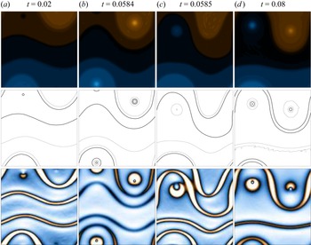
Figure 3 shows snapshots of the potential vorticity and speed fields at times  $t=0.02,0.0584,0.0585,0.08$ for the weakly forced case $n=26$. It shows the transition from an initial state dominated by three distinct jets to a later stage comprising two jets and two coherent vortices. As in figure 1, the contour levels have been selected to coincide with the jet cores but, importantly, the same levels have been used for all times.

Figure 3. Snapshots of the potential vorticity (top) and speed (bottom) fields for the weakly forced case  $ {k_D}=4$, $n=26$, $N=128$. Contours and colours are as in figure 1, with two contours highlighted in bold to facilitate identification between frames.
At the earlier time the two central jets span the  $x$ direction with relatively small undulations, while the jet near $y={\rm \pi}$ has a large meander around a nascent vortex. As the energy in the system increases, the meander of this jet becomes larger and vortices develop in each of its lobes. A sharp change in the topology of the flow (in the sense of the connectedness of isolines of vorticity) then occurs between $t=0.0584$ and $t=0.0585$, in which the upper of the two central jets ‘passes though’ the vortex in the left-hand half of the domain (the negative vortex). The structure at $t=0.0585$ then comprises one straight jet and two jets with a large meander around this vortex. From around $t=0.6$ to $t=0.8$, the two meandering jets gradually approach one another, smoothly and maintaining the same relative pattern, with a uniform propagation; there is only very slight adjustments to the potential vorticity levels and a gradual re-establishment of the positive vortex due to the continuous stochastic forcing. By time $0.08$ the two meandering jets have merged into a single jet meandering around the vortex pair.
Figure 4 shows the transition at  $t=0.584$ in more detail. As the middle jet in figure 3(b) approaches and interacts with the vortex, the flow becomes unstable, looses its stationarity and enters a highly transient state. The snapshots show the jets and coherent vortices interacting in a highly nonlinear and irregular way. Smaller scale waves are excited on all jets and persist for some time. (The time interval shown covers approximately ten translation periods of the pattern across the domain.) Gradually these smaller scale waves dissipate and the flow settles down into the state shown in figure 3(c), though some weak transience still persists even at this later time.

Figure 4. Snapshots of the potential vorticity (top) and speed (bottom) fields near time  $t=0.0584$ (a–d) for the weakly forced case $ {k_D}=4$, $n=26$, $N=128$. Colours are as in figure 1.
A similar change in the topology of the jet-vortex configuration is found to be associated with the drop in  $ {\mathcal {K}}$ near $t=0.3$. Figure 5 shows snapshots of the potential vorticity at $t=0.2,0.28,0.29, 0.5$ for the case $n=23$. At $t=0.2$, the flow comprises a weaker straight jet (near $y=-{\rm \pi}$) and a jet with a large meander around two coherent vortices. In the subsequent evolution, the straight jet develops an increasingly large meander, until around $t=0.29$ its left-hand lobe connects with and then passes though the negative vortex. The interaction involves the joining of the potential vorticity contour defining the jet with the outermost contour of the vortex, a topological change that cannot occur in a strictly inviscid flow. As in the case just examined, the transition is associated with the flow entering a highly transient state, here somewhat simpler that that shown in figure 4 involving irregular oscillations of the vortex within the meander lobe (not shown). The result is two jets of unequal strength meandering around the vortex pair, which then undergo a final merger into a single meandering jet. Again, this final merger is a gradual process involving the smooth and continual closing of the gap between the two jets. The pattern shown at $t=0.5$ is very stable and undergoes no further change in structure, with only a gradual extension of the meander and separation of the vortex pair in $y$ to the state at $t=1$ shown in figure 1(c) above.

Figure 5. Snapshots of the potential vorticity field for the case  $ {k_D}=4$, $n=23$, $N=128$. Contours are as in figure 3, with two contours again highlighted in bold. Fields have been offset in $x$ for clarity.
The topology, in the sense of the connectedness of isolines of the vorticity field, of the system comprising the two vortices and a single meandering jet may be classified as follows. If the pattern is shifted in  $y$ so that the negative vortex appears above (at larger $y$) the positive one (as in figure 1), we can distinguish between relatively straight jets that traverse the $x$ domain without meandering around the vortices, and strongly meandering jets that cannot be deformed into a straight line in the $x$ direction without passing through a vortex. For convenience, we refer to these as straight and meandering jets. Further, we may define a ‘full jet’ as one across which the potential vorticity jump is $2{\rm \pi}$. Thus, the states shown in figure 1 contain a meandering full jet, while the end state of figure 3 can be considered to contain a straight half-jet and a meandering half-jet.
Again with the negative vortex above the positive one, we can define the mode number of the state as the number of times a meandering jet crosses a notional horizontal line separating the vortices. The construction is illustrated in figure 1(c), an example of a mode-one state.
Following the case  $n=20$ beyond $t=1$, figure 6, the flow configuration evolves to increasing energy levels by increasing the length of the jet meander. Here, the green contours, at intervals of $q=2{\rm \pi}$, have been included to indicate the steepest gradients of potential vorticity and approximate location of the jets. By $t=2$, the separation between the vortices has increased by an amount approaching $2{\rm \pi}$, possible only because of the periodicity in $y$, with a corresponding increase in jet meander. The mode number has increased to two. The changes between $t=0.5$ (not shown, but very similar to the case $n=23$ in figure 5d) and around $t=3$ are continuous and involve no changes in the topology of the pattern. Viewed as a flow on a torus, the jet is being stretched around the torus in the poloidal direction by the vortices, but such that the global winding number on the torus remains zero.

Figure 6. Snapshots of the potential vorticity field at  $t=0.2$ and then selected times between $t=3.33T$ and $t=3.85T$ (a–h) for the case $ {k_D}=4$, $n=20$, $N=128$. Interval between green contours is $2{\rm \pi}$. Fields are offset in $x$ for clarity.
A series of repeated topological transitions begins around time  $t=3.33$. The descending lobe of the meander extends further towards the positive vortex (panel b), with which it connects, becoming contiguous with the outer vorticity levels of the vortex. The part of the jet immediately adjacent to the vortex then pinches off from the main jet and forms a distinct closed loop around the vortex (c). The vortex itself is now smaller and more compact than before the event, having lost peripheral material to the loop. Snapshots of the speed field (not shown) confirm that the loop and vortex are two distinct flow features at this time. The loop then gradually contracts toward the vortex until the two flow features recombine into a single vortex (d). At this time the descending lobe is again extending towards the vortex in the early stages of a second jet-vortex-loop interaction (e) that follows a similar sequence, which is followed by a third (g). Again, there is significant transience during and immediately after the jet-vortex interactions, characterized by undulations of the loop and vortex. In contrast, the contraction of the loop onto the vortex (c,d, etc) is a relatively gradual and smooth process.
The evolution across these times is suggestive of a periodic solution and the transition from quasi-steady to periodic behaviour at  $t=3.33$ may be viewed as bifurcation of the system as the energy increases beyond a critical point. Because the energy is increasing slowly over the period of oscillations, the evolution cannot be truly periodic: as energy grows further, a bifurcation to another type of solution seems likely. It remains to be tested whether fixing the energy at the level measured at $t=3.5T$, for example, would result in a continued sequence of more nearly periodic states. Non-negligible energy dissipation by the hyperdiffusion at these resolutions, at a level that is not easily controllable, complicates the construction of such an experiment slightly, which is left for future study.
3.2. Case $ {k_D}=16$

The behaviour at  $ {k_D}=16$ is broadly similar to that at $ {k_D}=4$. Figure 7 shows the growth of energy and enstrophy with time for cases with $n=24$ and $n=27$. At this $ {k_D}$, nearly all the energy resides in the potential part, and the potential and total energies are indistinguishable on the plot. The kinetic energy grows nearly monotonically, particularly at higher $n$, with isolated jumps to lower levels, again associated with topological changes in the flow structure. The quasi-periodic states that developed around $t\gtrsim 3T$ at $ {k_D}=4$ are not present at $ {k_D}=16$ over the extended time range considered.

Figure 7. Total (black), kinetic ( $ {k_D}^2 {\mathcal {T}}$, red) and potential ( $ {\mathcal {P}}$ green) energies and enstrophy (blue) as a function of time. Note that because $ {k_D}$ is large, the total and potential energies are indistinguishable on the plot, and $ {\mathcal {T}}$ is a very small residual.
Figure 8 shows snapshots of the potential vorticity for the case  $ {k_D}=16$, $n=27$, illustrating the flow changes associated with the drops in kinetic energy around $t=0.6$ (top row) and $t=0.8$ (bottom row). The green contours, at intervals of $q=2{\rm \pi}$, have again been included at the approximate location of the jets. Despite the regions of strong potential vorticity gradients being less well separated, the speed field (not shown) indicates that the jets are indeed distinct flow features, though only marginally so in the lower row, where the limited numerical resolution makes them somewhat diffuse. At $t=0.61$, the ascending lobe (right) approaches the negative vortex, and then merges with the outer part of its vorticity distribution. By $t=0.62$, the combination of jet with outer vortex separates from the vortex core and emerges as part of a single jet meander around the vortex, which has lost material in the process. The mode number has increased from two to three in the process. In contrast to times prior to $t=0.55$, where the mode number increases due to a gradual extension of the meander length, the increase to mode three at $t=0.61$– $0.62$ is due to a sudden change in the topology of the jet-vortex configuration. In fact, at the end of the transition the two vortices have moved closed together.

Figure 8. Snapshots of the potential vorticity field at selected times between  $t=0.55T$ and $t=0.82T$ (a–h) for the case $ {k_D}=16$, $n=27$, $N=128$. Orange is positive, blue is negative. The interval between green contours is $2{\rm \pi}$. Fields are offset in $x$ for clarity.
A similar transition occurs beginning at  $t=0.77$, again with the extension of the ascending lobe towards the negative vortex. This time the jet and vortex merge to form a closed loop around the vortex core, similar to the loop formation seen in figure 6. Now, however, the loop does not shrink back toward the vortex but rejoins the original jet lobe, remaining distinct from the vortex core. The transition involves an increase in mode number from three to four; it differs from the transition from mode two to three only in the formation of the intermediate loop at $t=0.78$. Note that the mode four structure is only just visible at this resolution, which marginally resolves the four jets traversing the horizontal line separating the vortices. A higher resolution would be needed to confirm the existence of a mode four state, or rule out the presence of quasi-periodic oscillations like those found at $ {k_D}=4$. It should also be acknowledged that such high mode number states on the $y$-periodic domain are of doubtful practical relevance to actual geophysical flows.
Similar topological changes occur at early times. Figure 9 shows the potential vorticity at times from  $t=0.04$ to $t=0.4$ for the case $n=30$, $ {k_D}=16$. Coloured regions in the top row highlight two jets, one relatively straight (dark pink), the other meandering (light blue). At $t=0.07$ the straight jet has merged and passed through the positive vortex (dark pink) leaving a smaller vortex core. There are now two meandering jets, each with a potential vorticity jump of ${\rm \pi}$. The light/dark pink at $t=0.07$ represents a single jet structure, but with a potential vorticity level differing by $2{\rm \pi}$ (due to non-periodicity of $q$). Similarly for the light/dark blue. At $t=0.07$– $0.09$, the ascending lobe (light pink) merges with and passes through the negative vortex (light pink). At $t=0.09$– $0.11$ the descending (dark blue) lobe of the other jet merges with and passes through the positive vortex.

Figure 9. Snapshots of potential vorticity at selected early times between  $t=0.04T$ and $t=0.4T$ (a–h) for the case $ {k_D}=16$, $n=30$, $N=128$. Contour interval is ${\rm \pi} /2$. Selected regions have been coloured for identification (see text). Fields are offset in $x$ for clarity.
In terms of the mode number defined above, we may consider the flow in (a) as mode  $\tfrac 12$, since the potential vorticity jump across the meandering jet is only ${\rm \pi}$. Similarly, the flow in (b) can be considered as mode $\tfrac 22$, comprising two distinct half-jets, and that in (c) as mode $\tfrac 32$. In panel (d) the merger of the dark-blue jet and vortex tail might be expected to give mode $\tfrac 42$. However, at this point the two half-jets merge into a single full jet and, in the process, the excursion of the jet meander decreases so that the positive vortex moves up beyond the level of the negative one. When the plot is shifted such that the negative vortex appears above the positive one, the flow is seen to have dropped back to mode 1.
Beyond this time the flow remains in integral mode numbers. Beyond  $t=0.16$ (e) the negative vortex again moves above the positive one and the flow is mode 2 ( f,g). (Here, shading is such that successively darker shades of pink represent potential vorticity ranges increasing by $2{\rm \pi}$). At $t=0.4$ (h), the descending lobe again approaches the positive vortex and a subsequent merger occurs, eventually resulting in a mode-3 pattern at a slightly later time (not shown).
3.3. Case $ {k_D}\le 2$

Qualitatively different late-time states are obtained for  $ {k_D}\le 2$. Figure 10 shows the potential vorticity for the case $ {k_D}=2$, $n=21$. At $t=0.31$ the flow comprises two half-jets in a mode- $\tfrac 12$ configuration similar to those obtained at $ {k_D}=4$ and $ {k_D}=16$ (compare figures 5a and 9a). Soon after, however, first the negative vortex disappears (b) while the meander length increases slightly. At the same time, the relatively straight jet develops an increasing meander resulting in the merger of the two half-jets. At this point the meandering jet abruptly straightens while two vortices establish themselves in the region of mixed potential vorticity. The rest of the evolution (c,d) consists simply of a gradual strengthening of these vortices as the energy in the flow increases. The single jet remains relatively straight (mode 0) throughout.

Figure 10. Snapshots of potential vorticity at selected times between  $t=0.31T$ and $t=T$ (left to right) for the case $ {k_D}=2$, $n=21$, $N=128$. Contour interval is ${\rm \pi} /2$.
Figure 11 shows a similar evolution for  $ {k_D}=1$, here with $n=19$, although the early time meandering jet is less clearly defined. Again from $t=0.5$ the flow assumes a configuration comprising a single straight jet plus a vortex dipole, in which energy increases purely through the strengthening of the vortices, with no meanders developing on the jet.

Figure 11. Snapshots of potential vorticity at selected times between  $t=0.2T$ and $t=T$ (left to right) for the case $ {k_D}=1$, $n=19$, $N=128$. Contour interval is ${\rm \pi} /2$.
4. Conclusions
The large-energy limit of weakly forced, late-time  $\beta$-plane turbulence has been considered. The flow is weakly forced in the sense that $ {L_{Rh}}/ {L_{\varepsilon }}\gg 1$ so that the potential vorticity assumes an approximate staircase structure, and has large energy in the sense that the jet spacing is equal to the domain width so that no further jet mergers can occur. The flows obtained in the numerical experiments performed are quasi-steady, with a very slow, linear growth in total energy: at $n=23$, $ {k_D}=4$, for instance, there is a fractional energy increase of the order of $10^{-5}$ in the time it takes a meander to propagate in $x$ once across the domain. In particular, the flows appear remarkably stationary over time scales that are short relative to $T$ but still long compared with, say, a Rossby wave period or vortex turnaround time. They suggest the existence of exact, steadily translating solutions comprising a single jet and vortex dipole. The configuration of these states depends on the deformation radius, with a relatively straight jet ultimately found for $ {k_D}\le 2$, and a strongly meandering jet, looping around the vortices for $ {k_D}\ge 4$. In the latter cases, the jet may traverse the entire domain in the $y$ direction one or more times, giving a jet orientation that is predominantly north–south, rather than the usually considered east–west. In these meandering cases, a mode number can be defined that quantifies the degree of meandering relative to the vortices.
The solutions appear to be numerically converged in the sense that the structures appear robust with increasing resolution. However, the experiments have been run at a relatively low resolution that clearly limits the representation of across-jet potential vorticity gradients. These gradients steepen as resolution increases, and it is expected that details such as the profiles of the coherent vortices will also depend on increasing resolution.
In extended simulations, where the energy levels are allowed to increase still further, a new regime was obtained in which the jet underwent successive transient interactions with one of the vortices. It is speculated that this oscillating state may be due to the existence of a periodic solution, resulting from a destabilization of the steadily translating jet-dipole structure as the energy exceeds a threshold. Establishing such a periodic solution will be considered in a future study of exactly stationary flows. Calculations in which the energy input rate is balanced by frictional damping would require much longer integration times to reach a true equilibrium. An alternative is to use time-varying forcing (as in Scott Reference Scott2023) with a decreasing in time energy input rate; however, significant energy loss to hyperdiffusion at these resolutions complicates the a priori specification of energy level.
The system also shows some evidence of hysteresis and bistable states. Preliminary calculations were carried out with an initial condition corresponding to the  $t=0.3$ state of the case $ {k_D}=4$, $n=23$, just after the transition shown in figure 5. The forcing was held the same as before, but a weak friction was introduced to reduce the energy level gradually over time. As the energy moved through the level corresponding to the transition at $t=0.28$, the flow remained as a single jet meandering around the two vortices. As the energy reduce further, this state persisted with a gradual reduction in the meander length, but no topological change to a two jet state. A more complete analysis of bistability, and the identification of exactly stationary solutions as indicated above, is underway and will be reported separately.
At energy levels less than, but approaching the large-energy limit, when two or three distinct jets still exist, the simulations show jet mergers that often involve a topological change in the configuration of the meandering jets and their embedded vortices. Jet merger in these cases proceeds via a highly transient interaction between the jet and the vortex, such that the jet first passes through the vortex, incorporating material from the vortex tails. The merger then occurs with the newly adjacent jet following the interaction.
The results presented here are particular to the doubly periodic geometry considered. On a finite planet, jet meanders cannot grow indefinitely, and the large mode number states in particular are of questionable geophysical relevance. However, the interaction between the meandering jet and vortex dipole nonetheless suggests patterns that might be obtained in a spherical geometry, and which may be more relevant to planetary flows under appropriate forcing conditions.
Declaration of interest
The authors report no conflict of interest.


 Open access