


1. Introduction
Turbulent boundary layers (TBLs) on streamlined geometries often experience strong pressure gradients and streamline curvature and are ubiquitous in engineering applications (e.g. submarine hulls, airfoils, airplane fuselages). Therefore, it is not surprising that the study of such boundary layers remains an active area of research. This paper has two main objectives: (i) to provide a new perspective on curved boundary layer analysis by deriving the Navier–Stokes equations in axisymmetric streamline coordinates; and (ii) to apply these equations to study the turbulent boundary layer of the axisymmetric DARPA SUBOFF hull at  $Re_L = 1.1 \times 10^{6}$. Wall-resolved large-eddy simulation (LES) of the flow over the SUBOFF hull is performed using the recently developed unstructured overset method of Horne & Mahesh (Reference Horne and Mahesh2019a,Reference Horne and Maheshb). To the best of our knowledge, this is the first time analysis in a streamline coordinate system has been applied to external flow about a streamlined body.
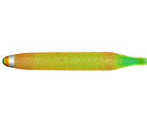
The DARPA SUBOFF hull (Groves, Huang & Chang Reference Groves, Huang and Chang1989) is a canonical body of revolution that is widely used for research purposes. The majority of canonical bodies of revolution have purely convex geometry, but this is not the case for the SUBOFF hull form, which has an inflection point in the surface curvature where the body switches from convex to concave curvature at the stern. Figure 1 shows the axisymmetric bare hull configuration of the SUBOFF. The tapering geometry at the tail of axisymmetric bodies such as the SUBOFF hull causes the incoming boundary layer to experience strong streamwise pressure gradients and makes streamlines in the plane of symmetry diverge in order to satisfy mean continuity as the streamlines converge axisymmetrically. The effect of the longitudinal streamline curvature is to create additional streamline-normal pressure gradients so that the pressure varies significantly across the boundary layer, as observed by Patel, Nakayama & Damian (Reference Patel, Nakayama and Damian1974). As a result, the streamwise pressure gradients may also vary significantly across the boundary layer in regions of the flow with varying streamline curvature. The axisymmetric convergence of streamlines at the tail of the body produces an extra strain rate, which in combination with the convex surface curvature strongly affects the flow field (Smits & Joubert Reference Smits and Joubert1982). Additionally, the transverse curvature of axisymmetric bodies becomes increasingly important, as the thickness,  $\delta$, of the rapidly growing boundary layer may quickly exceed the local radius of the body, $a$.
$a$.
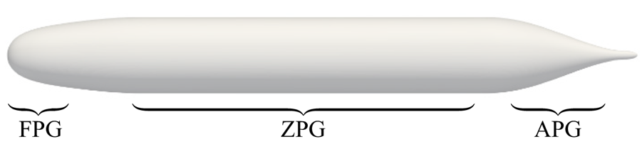
Figure 1. Visualization of the axisymmetric bare DARPA SUBOFF hull configuration. Favourable- pressure-gradient (FPG), zero-pressure-gradient (ZPG) and adverse-pressure-gradient (APG) regions are labelled.
In studying curved geometries, the choice of coordinate system presents some challenges. Most studies use either the base coordinate frame ( $x, r, \theta$) or a coordinate system aligned with the normal and tangential directions of the surface of the body, as in Tanarro, Vinuesa & Schlatter (Reference Tanarro, Vinuesa and Schlatter2020). While convenient, these coordinate systems have some limitations when studying boundary layer development. For the ( $x, r, \theta$) coordinate system, the no-penetration boundary condition on the body surface is not aligned with a coordinate direction for tapering geometries. As a result, the $x$ and $r$ velocities and derivatives with respect to $x$ and $r$ become of the same order in the governing equations, prohibiting typical boundary layer approximations. Surface-normal coordinates eliminate this problem and may be considered a good solution for thin boundary layers where the mean flow streamlines closely follow the contours of the body of interest. Patel (Reference Patel1973) presented boundary layer equations for the surface-normal coordinate system.
However, bodies with concave longitudinal curvature or thick boundary layers challenge the interpretation of surface-normal measurements. Streamlines in thick boundary layers at the tail of streamlined bodies are typically not aligned with the curvature of the body, so analysis of boundary layer development in surface-normal coordinates will struggle to describe the development of the flow. Surface-normal lines at the front of the geometry extend in the upstream direction, while lines at the stern extend in the downstream direction, causing the dominant velocity to switch between the wall-normal and wall-parallel components at some point outside the boundary layer. To summarize, in general, surface-normal coordinates do not align with the streamwise velocity. Finally, for bodies with concave longitudinal curvature (e.g. DARPA SUBOFF hull), two adjacent surface-normal lines must intersect at some point in the flow field, which may be close to or within the boundary layer. Clearly this poses a problem for the analysis of boundary layer development. It also prohibits contours to be plotted in the plane of symmetry because the velocity components are not uniquely defined in areas of the flow field where surface-normal lines intersect.
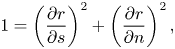
An ideal coordinate system would be both normal to the surface of the body and perpendicular to the free-stream velocity at large distances from the body, permitting analysis in the most natural frame of reference. The coordinate system must also allow the faithful analysis of streamline curvature for thick boundary layers attached to curved bodies, where the streamlines may not closely follow the curvature of the body. These requirements are satisfied by the streamline coordinate system derived by Finnigan (Reference Finnigan1983) for two-dimensional flows. His analysis defines a function  $\phi$, which reduces to the velocity potential for irrotational flows. Lines of constant $\phi$ satisfy the above requirements for analysis of curved bodies. The resulting orthogonal coordinate system from the streamline coordinate derivation is defined by $\phi$, the streamfunction $\psi$ and the plane of symmetry.
Figure 2 shows comparisons of radial, wall-normal and streamline-normal coordinate lines for the SUBOFF hull. From figure 2(a), we can see that the three coordinates are nearly identical over the zero-pressure-gradient (ZPG) mid-hull: the wall-normal and radial lines exactly coincide and closely match the streamline-normal lines, since the radial velocity is small in this region. Over the front and stern of the hull, there are differences between the three coordinate lines. On the front of the hull (figure 2b), the wall-normal and streamline-normal lines are perpendicular to the hull surface at the wall and coincide for most of the thin boundary layer, whereas the radial lines increasingly diverge from the surface near the stagnation point. Outside of the boundary layer, the wall-normal and streamline-normal lines begin to diverge, as the streamline-normal lines curve to become parallel with the radial direction far from the body, while the wall-normal lines extend in the upstream direction. At the stern (figure 2c), the thick boundary layer guides the curvature of the streamline-normal lines away from the wall-normal coordinate within the boundary layer. We also see from figure 2(a) that the wall-normal lines do indeed intersect in the fluid domain due to the concave curvature of the hull surface.
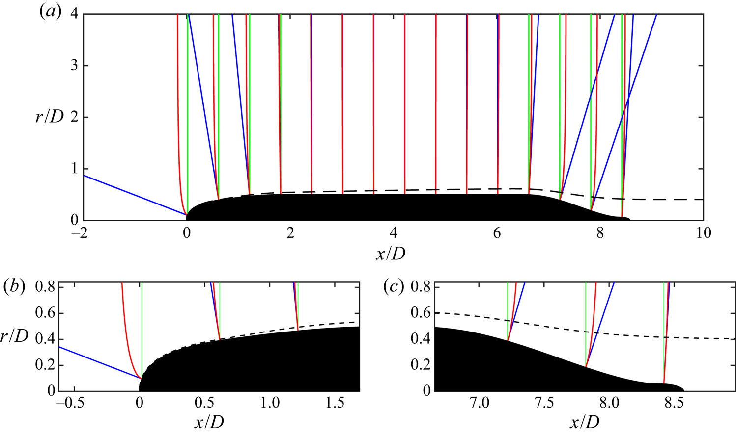
Figure 2. (a) Comparison of the radial (green), wall-normal (blue) and streamline-normal (red) lines for the SUBOFF hull geometry along with the boundary layer edge (– – – –). Panels (b) and (c) show detailed views of the coordinate lines in the boundary layer at the front (b) and stern (c) of the hull.
It will be shown that rewriting the Navier–Stokes equations in the streamline coordinate system has several benefits. First, the terms in the resulting equations now explicitly describe transport along or normal to streamlines, eliminating the ambiguity of coordinates not aligned with the mean flow and defining the Reynolds shear stress to directly represent the turbulent transport of momentum across streamlines. The momentum equations also naturally reduce to the differential form of Bernoulli's equation and the Euler equation for curved streamlines outside of the boundary layer, which is valuable in the analysis of curved geometries. This also allows any set of two-dimensional boundary layers to be directly compared. Finally, a result of the transformation to the new coordinate system is the appearance of acceleration, streamline curvature and streamline convergence length scales in the Reynolds-averaged Navier–Stokes equations, which may aid in analysis of streamline curvature effects. Finnigan et al. (Reference Finnigan, Raupach, Bradley and Aldis1990) applied the two-dimensional streamline equations derived by Finnigan (Reference Finnigan1983) to analyse flow over a hill, but few subsequent studies have taken advantage of the streamline coordinate system until somewhat recently. Saxton-Fox et al. (Reference Saxton-Fox, Ding, Smits and Hultmark2019) studied the deformation of structures in a turbulent pipe flow with various streamlined axisymmetric bodies placed at the centreline. In analysing the same configuration, Ding et al. (Reference Ding, Saxton-Fox, Hultmark and Smits2019) examined the redistribution of momentum and Reynolds shear stress using coordinates aligned with streamlines and potential lines, although analysis of the governing equations was performed in the Cartesian frame. Recently Yousefi & Veron (Reference Yousefi and Veron2020) derived streamline flow equations for flow over waves by decomposing the two-dimensional equations into mean, wave-induced and turbulent components. Yousefi, Veron & Buckley (Reference Yousefi, Veron and Buckley2020) demonstrated the value of these equations by applying them to study the contribution to the momentum budget by these three sources for wind over periodic waves.
The conversion to streamline coordinates also has drawbacks. The coordinate system is now curved in multiple directions, with the coordinate directions changing at different locations in the flow field and partial derivatives replaced by directional derivatives. Additionally, the practicality of the analysis is limited in that it requires knowledge of the flow field to define the coordinate system and perform measurements in the directions aligned with the mean flow. Finally, the streamline coordinate system is not applicable for analysis of separated flows or recirculation bubbles and is limited to flows that can be defined by two orthogonal stream surfaces and a third surface normal to them (e.g. the plane of symmetry) in order to produce an orthogonal coordinate system. Finnigan (Reference Finnigan1983) establishes that this condition is satisfied for a complex lamellar velocity field where the mean vorticity vector is normal to the mean velocity vector, that is,  $\boldsymbol {U} \boldsymbol {\cdot } (\boldsymbol {\nabla } \times \boldsymbol {U} ) = 0$. Both two-dimensional and axisymmetric flows are complex lamellar, and the analysis of Finnigan (Reference Finnigan1983) focuses solely on the two-dimensional case. While the streamline coordinate system has features that limit its applicability to general problems, it is certainly valuable for developing an understanding of a wide variety of complex flows.
The flow around the stern of the SUBOFF hull has a variety of competing effects, including pressure gradients, streamline curvature, transverse curvature and streamline convergence. Bradshaw (Reference Bradshaw1973) summarized several studies of streamline curvature, noting that even relatively small streamline curvature can have surprisingly large effects on the turbulent field. Patel & Sotiropoulos (Reference Patel and Sotiropoulos1997) later summarized experimental studies and turbulence models that attempted to explain the effects of longitudinal curvature on momentum transport in turbulent boundary layers.
The effects of transverse curvature pertaining to axisymmetric TBLs have received less attention than flat-plate TBLs but nevertheless have been studied in a variety of regimes (Lueptow, Leehey & Stellinger Reference Lueptow, Leehey and Stellinger1985; Lueptow Reference Lueptow1990; Neves, Moin & Moser Reference Neves, Moin and Moser1994; Jordan Reference Jordan2011, Reference Jordan2015). The effects of transverse curvature for TBLs on cylinders was summarized by Piquet & Patel (Reference Piquet and Patel1999). They identified three flow regimes depending on the ratio of the boundary layer thickness to the radius of the axisymmetric body ( $\delta /a$) and the radius of curvature in wall units ( $a^{+}$). Kumar & Mahesh (Reference Kumar and Mahesh2018a) extended the integral analysis of Wei, Maciel & Klewicki (Reference Wei, Maciel and Klewicki2017) to axisymmetric boundary layers, confirming the experimental observation that skin friction increased for an axisymmetric boundary layer compared to a flat plate.
Smits, Eaton & Bradshaw (Reference Smits, Eaton and Bradshaw1979a) studied the effects of axisymmetric lateral divergence over a cylinder–flare body, finding that the combination of the lateral divergence and concave curvature at the transition to the flare destabilized the turbulence and increased the turbulence intensity throughout the boundary layer, as opposed to streamline curvature alone (Smits, Young & Bradshaw Reference Smits, Young and Bradshaw1979b). Patel et al. (Reference Patel, Nakayama and Damian1974) studied the thick boundary layer at the tail of a body of revolution, finding that there was a significant variation of static pressure in the boundary layer and the thick boundary layer was characterized by an abnormally low level of turbulence and a strong interaction with the outside potential flow. Smits & Joubert (Reference Smits and Joubert1982) studied flow about a body of revolution and compared it to flow about a two-dimensional wing that was designed to have the same pressure distribution as the axisymmetric body and modified to have the same longitudinal surface curvature. They concluded that there was a strong interaction between the two additional rates of strain arising from the longitudinal surface curvature and the lateral convergence produced by the axisymmetric body. Recently, Balantrapu et al. (Reference Balantrapu, Hickling, Millican, Vishwanathan, Gargiulo, Alexander, Lowe and Deveport2019) studied the development of a thick stern boundary layer on the  $20^{\circ }$ tail cone of a body of revolution, finding that the large-scale turbulent motions in the outer portion of the boundary layer are amplified by the adverse pressure gradient.
Axisymmetric bodies with inflection points have been studied in the past by Huang, Groves & Belt (Reference Huang, Groves and Belt1980). Posa & Balaras (Reference Posa and Balaras2016, Reference Posa and Balaras2020) studied the appended SUBOFF hull at length-based Reynolds numbers  $Re_L = 1.2 \times 10^{6}$ and $Re_L = 1.2 \times 10^{7}$, finding that the peak of turbulent kinetic energy was shifted away from the wall to form a double-peaked profile of turbulent stresses in the wake. Kumar & Mahesh (Reference Kumar and Mahesh2018b) performed LES on the bare hull configuration of the SUBOFF geometry, witnessing the same behaviour of turbulence quantities in the wake and commenting on the higher skin friction and higher radial decay of turbulence from the wall compared to flat-plate TBLs.
This paper is organized as follows. Next, § 2 defines the axisymmetric streamline coordinates and the Navier–Stokes equations in this coordinate system. The details of the numerical method and computational set-up for overset LES of the axisymmetric SUBOFF hull are given in § 3. Results and insights from the streamline coordinate system are discussed in § 4. A brief summary in § 5 concludes the paper.
2. The axisymmetric streamline coordinate system
In this section, we first introduce the streamline coordinate system in § 2.1 and then transform the Reynolds-averaged Navier–Stokes momentum equations into axisymmetric streamline coordinates in § 2.2.
2.1. Definition of the coordinate system
The streamline coordinate system is defined by the normal intersection of three surfaces  $(x_1, x_2, x_3)$ defined by the cylindrical coordinates $(y_1, y_2, y_3) = (x, r, \theta )$. These are
 \begin{equation}
\left.\begin{gathered} x_3 = \theta
=\textrm{const., the plane of
symmetry}, \\ x_2 = \psi (x, r)
=\textrm{const.,
the
streamfunction}, \\ x_1 = \phi (x, r)
=\textrm{const., the surface
normal to } x_2 \textrm{ and }x_3.
\end{gathered}\right\}
\end{equation}
\begin{equation}
\left.\begin{gathered} x_3 = \theta
=\textrm{const., the plane of
symmetry}, \\ x_2 = \psi (x, r)
=\textrm{const.,
the
streamfunction}, \\ x_1 = \phi (x, r)
=\textrm{const., the surface
normal to } x_2 \textrm{ and }x_3.
\end{gathered}\right\}
\end{equation}
The streamfunction  $\psi$ is defined in the traditional form for the cylindrical coordinate system as
 \begin{equation} U_x = \frac{1}{r} \frac{\partial \psi}{\partial r}, \quad U_r ={-} \frac{1}{r} \frac{\partial \psi}{\partial x}, \end{equation}
where  $U_x$ and $U_r$ are the mean velocity components in the $x$ and $r$ directions, respectively. Since $\phi$ is normal to $\psi$, the tangents of the $\phi = \textrm {const.}$ lines are proportional to $\boldsymbol {\nabla } \psi$, so they must satisfy
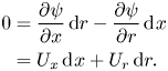 \begin{align} 0 &= \frac{\partial \psi}{\partial x}\,\textrm{d}r - \frac{\partial \psi}{\partial r}\,\textrm{d}\kern0.7pt x \nonumber\\ &= U_x \,\textrm{d}\kern0.7pt x + U_r \,\textrm{d}r. \end{align}
 A solution to this ordinary differential equation is known to exist for complex lamellar flows, as we have in the present case. This means there must exist an integrating factor  $\zeta$ such that
 \begin{equation} ( \zeta U_x ) \,\textrm{d}\kern0.7pt x + ( \zeta U_r ) \,\textrm{d}r = 0 = \textrm{d}\phi , \end{equation}
which implies that
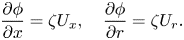 \begin{equation} \frac{\partial \phi}{\partial x} = \zeta U_x, \quad \frac{\partial \phi}{\partial r} = \zeta U_r. \end{equation}
Therefore, the streamline coordinate system is fully defined as long as we are able to determine the integrating factor  $\zeta$. Finnigan (Reference Finnigan1983) provides insight into the meaning of $\zeta$ by expressing the orthogonality condition as $\boldsymbol {\nabla } \phi = \zeta \boldsymbol {\nabla } \times \boldsymbol {\varPsi }$, where $\boldsymbol {\varPsi } = (0, 0, \psi )$ is the vector potential. A constraint on $\zeta$ is obtained by using the vector identity
 \begin{equation} 0 = \boldsymbol{\nabla} \times \boldsymbol{\nabla} \phi = \boldsymbol{\nabla} \times ( \zeta \boldsymbol{\nabla} \times \boldsymbol{\varPsi} ). \end{equation}
For cylindrical coordinates, this is equivalent to
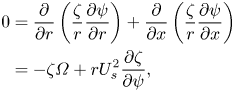 \begin{align} 0 &= \frac{\partial}{\partial r} \left( \frac{\zeta}{r} \frac{\partial \psi}{\partial r} \right) + \frac{\partial}{\partial x} \left( \frac{\zeta}{r} \frac{\partial \psi}{\partial x} \right) \nonumber\\ &={-} \zeta \varOmega + r U_s^{2} \frac{\partial \zeta}{\partial \psi}, \end{align}
where the velocity magnitude (streamwise velocity),  $U_s$, and the single component of mean vorticity, $\varOmega$, are defined by $U_s^{2} = U_x^{2} + U_r^{2}$ and $\varOmega = \partial U_r/\partial x - \partial U_x/\partial r$. The constraint on $\zeta$ is therefore
 \begin{equation} \frac{1}{\zeta} \frac{\partial \zeta}{\partial \psi} = \frac{\partial ( \ln \zeta )}{\partial \psi} = \frac{\varOmega}{r U_s^{2}}. \end{equation}
 In a similar result to Finnigan (Reference Finnigan1983), we see that for irrotational flows  $\varOmega = 0$, and therefore $\zeta = \textrm {const.}$, which may be set equal to one. In this case (2.5a,b) become the potential function in cylindrical coordinates. In general, $\zeta$ depends on the shape of the streamlines, but the final result of the transformed equations has no dependence on $\zeta$ for steady streamlines through application of (2.8) in the coordinate transformation process.
2.2. Transformation of the Navier–Stokes equations into the streamline coordinate frame
We now derive the streamline coordinate equations for axisymmetric flow in a similar fashion to the two-dimensional case from Finnigan (Reference Finnigan1983). While the analysis for two-dimensional flow requires a single transformation from the Cartesian frame to the streamline coordinate frame, the axisymmetric streamline coordinate system requires a transformation from Cartesian to cylindrical coordinates, followed by a second transformation to axisymmetric streamline coordinates. A result of these transformations is that the radius from the axis of symmetry,  $r$, remains in the final streamline coordinates as an additional length scale.
The contravariant components of the streamline, cylindrical and Cartesian frames are
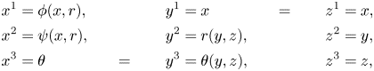 \begin{align}
\begin{aligned}
x^{1} &= \phi (x,r), & y^{1} &= x &\quad=\qquad z^{1} &=x, \\
x^{2} &= \psi (x,r), & y^{2} &= r(y,z), & z^{2} &= y, \\
x^{3} &= \theta &\quad= \qquad y^{3} &= \theta (y,z), & z^{3} &= z, \end{aligned}
\end{align}
\begin{align}
\begin{aligned}
x^{1} &= \phi (x,r), & y^{1} &= x &\quad=\qquad z^{1} &=x, \\
x^{2} &= \psi (x,r), & y^{2} &= r(y,z), & z^{2} &= y, \\
x^{3} &= \theta &\quad= \qquad y^{3} &= \theta (y,z), & z^{3} &= z, \end{aligned}
\end{align}
where the  $y^{1} = z^{1} = x$ coordinate is the axis of symmetry. The relations between the coordinate systems are defined by
 \begin{equation} \left.\begin{array}{l@{}}
\dfrac{\partial \phi}{\partial x} = \zeta U_x ,\\[1pc]
\dfrac{\partial \phi}{\partial r} = \zeta U_r ,
\end{array}\quad \begin{array}{l} \dfrac{\partial
\psi}{\partial x} ={-} r U_r ,\\[1pc] \dfrac{\partial
\psi}{\partial r} = r U_x , \end{array}\quad
\begin{array}{l@{}} \dfrac{\partial r}{\partial y} =
\dfrac{y}{r} ,\\[1pc] \dfrac{\partial r}{\partial z} =
\dfrac{z}{r} , \end{array}\quad \begin{array}{l@{}}
\dfrac{\partial \theta}{\partial y} ={-} \dfrac{z}{r^{2}}
,\\[1pc] \dfrac{\partial \theta}{\partial z} =
\dfrac{y}{r^{2}}. \end{array}\right\}
\end{equation}
\begin{equation} \left.\begin{array}{l@{}}
\dfrac{\partial \phi}{\partial x} = \zeta U_x ,\\[1pc]
\dfrac{\partial \phi}{\partial r} = \zeta U_r ,
\end{array}\quad \begin{array}{l} \dfrac{\partial
\psi}{\partial x} ={-} r U_r ,\\[1pc] \dfrac{\partial
\psi}{\partial r} = r U_x , \end{array}\quad
\begin{array}{l@{}} \dfrac{\partial r}{\partial y} =
\dfrac{y}{r} ,\\[1pc] \dfrac{\partial r}{\partial z} =
\dfrac{z}{r} , \end{array}\quad \begin{array}{l@{}}
\dfrac{\partial \theta}{\partial y} ={-} \dfrac{z}{r^{2}}
,\\[1pc] \dfrac{\partial \theta}{\partial z} =
\dfrac{y}{r^{2}}. \end{array}\right\}
\end{equation}
These relations are used to evaluate the contravariant metric tensor  $g^{pq}$ using the chain rule to relate the streamline coordinates ( $x^{i}$) to the Cartesian coordinates ( $z^{i}$):
 \begin{equation} g^{pq} = \sum_i \frac{\partial x^{p}}{\partial z^{i}} \frac{\partial x^{q}}{\partial z^{i}} = \begin{pmatrix} \zeta^{2} U_s^{2} & 0 & 0 \\ 0 & r^{2} U_s^{2} & 0 \\ 0 & 0 & r^{{-}2} \end{pmatrix}. \end{equation}
 Next, we note that the covariant metric tensor  $g_{pq}$ is related to its contravariant counterpart by
 \begin{equation} g_{pq} = ( g^{pq} )^{{-}1} = \begin{pmatrix} \zeta^{{-}2} U_s^{{-}2} & 0 & 0 \\ 0 & r^{{-}2} U_s^{{-}2} & 0 \\ 0 & 0 & r^{2} \end{pmatrix}. \end{equation}
 To transform the Navier–Stokes equations, we must be able to transform the derivatives to the streamline frame. The covariant derivative with respect to the  $l{\textrm {th}}$ contravariant component is denoted by the subscript ‘ $_{,l}$’. The derivatives required for the equation transformations are:
(i) the covariant derivative of a scalar,
(2.13) \begin{equation} \alpha_{,l} = \frac{\partial \alpha}{\partial x^{l}}; \end{equation}
(ii) the covariant derivative of a contravariant vector,
(2.14)\begin{equation} a^{i}_{,l} = \frac{\partial a^{i}}{\partial x^{l}} + \varGamma_{kl}^{i} a^{k}; \end{equation}(iii) the covariant derivative of a contravariant tensor,
(2.15)\begin{equation} A^{ij}_{,l} = \frac{\partial A^{ij}}{\partial x^{l}} + \varGamma_{kl}^{i} A^{kj} + \varGamma_{kl}^{j} A^{ik}; \end{equation}(iv) the covariant derivative of a mixed tensor,
(2.16)\begin{equation} A_{j,l}^{i} = \frac{\partial A_j^{i}}{\partial x^{l}} + \varGamma_{kl}^{i} A_j^{k} - \varGamma_{jl}^{k} A_k^{i}. \end{equation}


In these equations,  $\varGamma _{jk}^{i}$ is the Christoffel symbol of the second kind, defined by
 \begin{equation} \varGamma_{jk}^{i} = \frac{1}{2} g^{ip} \left[ \frac{\partial g_{pj}}{\partial x^{k}} + \frac{\partial g_{pk}}{\partial x^{j}} - \frac{\partial g_{jk}}{\partial x^{p}} \right]. \end{equation}
For orthogonal coordinate systems, as in the present case, Bradshaw (Reference Bradshaw1973) details simpler expressions for  $\varGamma _{jk}^{i}$ using scale factors $h_i = (g_{ii})^{1/2}$ (no summation). These expressions are:
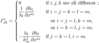 \begin{equation} \varGamma_{jk}^{i} =
\begin{cases} 0 & \text{if }
i, j, k \text{ are all different }; \\ \dfrac{1}{h_l} \dfrac{\partial
h_l}{\partial x^{m}} & \text{if }
i = j = k = l = m, \\ & \quad \text{or }
i = j = l, k = m, \\ &
\quad \text{or }i = k =
l, j =
m; \\ - \dfrac{h_l}{h_m^{2}}
\dfrac{\partial h_l}{\partial x^{m}} & \text{if }
j = k = l, i = m.\end{cases} \end{equation}
\begin{equation} \varGamma_{jk}^{i} =
\begin{cases} 0 & \text{if }
i, j, k \text{ are all different }; \\ \dfrac{1}{h_l} \dfrac{\partial
h_l}{\partial x^{m}} & \text{if }
i = j = k = l = m, \\ & \quad \text{or }
i = j = l, k = m, \\ &
\quad \text{or }i = k =
l, j =
m; \\ - \dfrac{h_l}{h_m^{2}}
\dfrac{\partial h_l}{\partial x^{m}} & \text{if }
j = k = l, i = m.\end{cases} \end{equation}
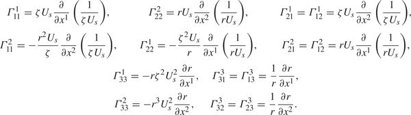
The non-zero Christoffel symbols calculated for the present transformation are provided in table 1.
Table 1. Non-zero Christoffel symbols for the metric tensor in (2.12).
It is important to note that the components of  $x^{i}$ in the final streamline coordinate system do not have units of length, having dimensions of $\mathrm {L}^{2}/\mathrm {T}$, $\mathrm {L}^{3}/\mathrm {T}$ and $0$, respectively. To produce equations with familiar quantities, the components of a given tensor $a^{i}$ must be transformed into its physical components $a(i)$. This allows the turbulence equations to be written in terms of physical components with quantities that can be readily understood and measured using a Cartesian frame locally tangent to the streamlines. This transformation to physical components is performed by
 \begin{equation} a(i) = ( g_{ii} )^{1/2} a^{i} = h_i a^{i} \quad \text{ (no summation)}. \end{equation}
This alteration of the equations is familiar in that the same transformation is required for the cylindrical  $(x, r, \theta )$ coordinate system. For example, in both the present and cylindrical coordinates, $\theta$ is an angle and therefore $\partial \theta / \partial t$ is not the component of velocity in the $\theta$-direction. We can see that applying (2.19) to this derivative produces the correct $\theta$-direction velocity of $r\partial \theta / \partial t$.
Using the above equations, we transform the equations into the new frame following the process detailed by Bradshaw (Reference Bradshaw1973). This process consists of the following steps:
(i) Write the equations for Cartesian coordinates in general tensor notation with ‘
$_{,l}$’ operators using the formulae provided by Bradshaw (Reference Bradshaw1973).(ii) Convert the ‘
$_{,l}$’ operators back into partial derivatives $\partial / \partial x^{i}$ in the new coordinate system using (2.13)–(2.16).(iii) Recover the physical components in the transformed equations using (2.19).


In writing the equations of motion in the streamline coordinate frame, we use the Reynolds decomposition to split the velocities and pressure into mean and fluctuating parts, denoted by capital and lower-case letters, respectively. The total velocity is therefore  $U^{i} + u^{i}$, and the sum of mean and fluctuating pressures is $P+p$, where by definition the average value of the fluctuating variables is zero. In the streamline coordinate system, the $x^{1}$ coordinate is aligned with the streamline (the direction of the mean velocity vector), and therefore $U^{2} = U^{3} = 0$. The axisymmetry of the flow also requires $\partial / \partial x^{3} = 0$. As in Finnigan (Reference Finnigan1983), the $x^{1}$ coordinate increases in the direction of the mean velocity vector, and a right-handed coordinate system is produced by the right-handed definition of vorticity. The result is that $U(1)$ is always positive, and is therefore the positive root of $U_s^{2}$, producing $U(1) = U_s$. In presenting the final equations in axisymmetric streamline coordinates, we denote the $x(1)$ and $x(2)$ coordinates with $s$ and $n$ to represent the physical distances along the streamline and streamline-normal trajectories, respectively. The velocity notation follows naturally with the total (mean plus fluctuating) velocities in the $s$-,
$s$-,  $n$- and $\theta$-directions defined as $U_s + u_s$, $u_n$ and $u_{\theta }$.
We first transform the continuity equation, since the result helps to illustrate the behaviour of the streamline coordinate system. The continuity equation for the mean velocity in general tensor form is
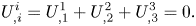 \begin{equation} U_{,i}^{i} = U_{,1}^{1} + U_{,2}^{2} + U_{,3}^{3} = 0. \end{equation}
Following the transformation steps for these three terms produces
 \begin{align} 0 &=\left( \frac{\partial U^{1}}{\partial x^{1}} + \varGamma_{11}^{1} U^{1} \right) + \varGamma_{12}^{2} U^{1} + \varGamma_{13}^{3} U^{1} \nonumber\\ &=\frac{\partial U_s}{\partial s} + \left(- \frac{\partial U_s}{\partial s} - \frac{U_s}{r} \frac{\partial r}{\partial s} \right) + \frac{U_s}{r} \frac{\partial r}{\partial s} = 0. \end{align}
This trivial result for continuity is intuitive, as the shape of the streamlines must inherently satisfy conservation of mass for the mean flow.
We follow by transforming the mean momentum equations into the axisymmetric streamline coordinate frame. The incompressible mean momentum equation in general tensor form, as provided by Bradshaw (Reference Bradshaw1973), is
 \begin{equation} \frac{\partial U^{i}}{\partial t} + U^{l} U_{,l}^{i} ={-} \frac{g^{il}}{\rho} P_{,l} - ( \overline{u^{l} u^{i}})_{,l} + \nu g^{kl} U_{,kl}^{i}. \end{equation}
The transformation of the momentum equations into the final streamline form is a bit laborious; the details are not particularly illuminating and are therefore omitted in the interests of clarity. Readers interested in adopting this coordinate system can find specifics of the transformation in Appendix A.
The final streamwise mean momentum equation is
 \begin{align} &\frac{\partial U_s}{\partial t} + U_s \frac{\partial U_s}{\partial s} + U_s \frac{\partial \ln(\zeta U_s)}{\partial t} \nonumber\\ &\quad ={-} \frac{1}{\rho} \frac{\partial P}{\partial s} - \frac{\partial \overline{u_s^{2}}}{\partial s} - \frac{\partial \overline{u_s u_n}}{\partial n} + \frac{\overline{u_s^{2}} - \overline{u_n^{2}}}{L_a} + \frac{2 \overline{u_s u_n}}{R_s} + \left( \overline{u_{\theta}^{2}} - \overline{u_n^{2}} \right) \frac{1}{r} \frac{\partial r}{\partial s} \nonumber\\ &\qquad - \overline{u_s u_n} \frac{1}{r} \frac{\partial r}{\partial n} + \nu \left[ \frac{ \partial^{2} U_s}{\partial s^{2}} +\frac{ \partial^{2} U_s}{\partial n^{2}} -\frac{2}{L_a} \frac{\partial U_s}{\partial s} -\frac{1}{R_s} \frac{\partial U_s}{\partial n} -\frac{U_s}{R_s^{2}}\right. \nonumber\\ &\qquad\left.-\frac{2}{r} \frac{\partial r}{\partial s} \frac{\partial U_s}{\partial s} +\frac{1}{r} \frac{\partial r}{\partial n} \frac{\partial U_s}{\partial n} -\frac{2 U_s}{r^{2}} \left( \frac{\partial r}{\partial s} \right)^{2} \right], \end{align}
where it is clear that the integrating factor  $\zeta$ disappears from the equations for steady flow, where the shape of the streamlines is stationary.
The mean advection terms are simplified in this coordinate system, although there are additional higher moment terms that involve two new length scales,  $L_a$ and $R_s$, expressed as curvatures $1/L_a$ and $1/R_s$. The curvature $1/L_a$ is defined by
 \begin{equation} \frac{1}{L_a} = \frac{1}{U_s} \frac{\partial U_s}{\partial s} = \frac{\partial \ln U_s}{\partial s}, \end{equation}
and  $L_a$ represents the e-folding length scale of streamwise accelerations, as well as the radius of curvature of streamline-normal coordinates. Conversely, the second length scale, $R_s$, is the local radius of curvature of the streamlines, defined by
 \begin{equation} \frac{1}{R_s} = \frac{1}{U_s} \left( \varOmega + \frac{\partial U_s}{\partial n} \right), \end{equation}
 where  $R_s$ is positive if the local centre of curvature is in the direction of increasing $n$. Rewriting the above equation, we see that as in ‘natural’ ( $s$–
$s$– $n$) coordinates, the mean vorticity consists of two terms,
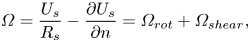 \begin{equation} \varOmega = \frac{U_s}{R_s} - \frac{\partial U_s}{\partial n} = \varOmega_{rot} + \varOmega_{shear}, \end{equation}
where  $U_s/R_s$ (the angular velocity of a fluid element along a streamline) is the vorticity contribution from rotation and $-\partial U_s / \partial n$ is the contribution from shear.
With the definitions of the additional length scales, the streamwise momentum equation contains explicitly the three radii that define the curvature of the coordinate system:  $r$,
$r$,  $R_s$ and $L_a$. Also, the additional terms in (2.23) that involve $r^{-1} \partial r / \partial s$ appear to be related to the lateral convergence or divergence of the streamlines (Smits et al. Reference Smits, Eaton and Bradshaw1979a), whereas the $\partial r / \partial n$ terms are related to the factors of $r$ that appear in derivatives for standard cylindrical Navier–Stokes equations. Note that $\partial r / \partial s$ and $\partial r / \partial n$ are related geometrically by
 \begin{equation} 1 = \left( \frac{\partial r}{\partial s} \right)^{2} + \left( \frac{\partial r}{\partial n} \right)^{2} , \end{equation}
but are left separate in the final equations for simplicity of notation.
The final streamline-normal mean momentum equation is
 \begin{align} \frac{U_s^{2}}{R_s} &={-} \frac{1}{\rho} \frac{\partial P}{\partial n} - \frac{\partial \overline{u_s u_n}}{\partial s} - \frac{\partial \overline{u_n^{2}}}{\partial n} + \frac{2 \overline{u_s u_n}}{L_a} + \frac{\overline{u_n^{2}} - \overline{u_s^{2}}}{R_s} + \overline{u_s u_n} \frac{1}{r} \frac{\partial r}{\partial s} \nonumber\\ &\quad + \left( \overline{u_{\theta}^{2}} - \overline{u_n^{2}} \right) \frac{1}{r} \frac{\partial r}{\partial n} + \nu \left[ - \frac{ \partial^{2} U_s}{\partial n \partial s} - \frac{1}{L_a} \frac{\partial U_s}{\partial n} + \frac{\partial}{\partial s} \left( \frac{U_s}{R_s} \right)+ \frac{U_s}{R_s L_a} \right.\nonumber\\ &\quad \left.- 2 \frac{\partial U_s}{\partial n} \frac{1}{r} \frac{\partial r}{\partial s} - \frac{\partial U_s}{\partial s} \frac{1}{r} \frac{\partial r}{\partial n} + \frac{U_s}{R_s} \frac{1}{r} \frac{\partial r}{\partial s} - \frac{U_s}{r^{2}} \frac{\partial r}{\partial n} \frac{\partial r}{\partial s} \right], \end{align}
where  $U_s^{2}/R_s$ on the left-hand side represents the centripetal acceleration of fluid elements along curved streamlines.
Examination of (2.23) reveals that the streamwise momentum equation reduces to the differential form of Bernoulli's equation for steady inviscid flow outside the boundary layer, while (2.28) reduces to the Euler equation for curved intrinsic coordinates. Additionally, it is readily verified that the equations naturally reduce to the cylindrical Reynolds-averaged Navier–Stokes equations for axisymmetric flow whose streamlines are aligned with the axis of symmetry.
3. Simulation details
These equations in the streamline coordinate system are applied to the analysis of flow about the axisymmetric DARPA SUBOFF hull at a Reynolds number of  $Re_L = 1.1 \times 10^{6}$ based on the length of the hull. The simulations are performed using wall-resolved LES, where the large turbulent scales are resolved and the small scales are modelled. In this section, we first describe the numerical method used for the present simulations in § 3.1, following which we detail the geometry, computational grid and domain sizing in § 3.2.
3.1. Numerical method
In the simulation of complex bodies at high Reynolds numbers, such as the present calculation, it is desirable that the numerical method remains robust without introducing numerical dissipation that would artificially damp small-scale turbulent motions. Mahesh, Constantinescu & Moin (Reference Mahesh, Constantinescu and Moin2004) developed a method for solving the incompressible flow equations on unstructured grids that emphasizes discrete kinetic energy conservation, ensuring robustness without added numerical dissipation. This property is essential for performing LES at high Reynolds numbers, since by definition the LES does not resolve the viscous dissipation on the computational grid and in general one cannot rely on the subgrid model to remove energy from the smallest scales at the correct rate to ensure numerical stability. The algorithm has successfully simulated a variety of complex flows (Verma, Jang & Mahesh Reference Verma, Jang and Mahesh2012; Jang & Mahesh Reference Jang and Mahesh2013; Kumar & Mahesh Reference Kumar and Mahesh2017, Reference Kumar and Mahesh2018b).
Horne & Mahesh (Reference Horne and Mahesh2019b) extended the method to allow for the overset simulation of arbitrarily overlapping and moving meshes in six-degrees-of-freedom motion. In an overset method, the simulation domain is composed of several overlapping body-fitted meshes. Redundant cells in overlapping adjacent meshes are removed, leaving exposed cells within the domain that require boundary conditions provided by interpolation of the solution between meshes. The ability of the overset method to simulate bodies with six degrees of freedom or prescribed movement is essential for the simulation of manoeuvring vehicles. However, even for simulation of stationary bodies (as in the present case), the overset method offers advantages. The method allows body-fitted meshes to be tailored to capture the fine near-wall scales, while allowing greater flexibility for grid refinement and lowering computational cost in the far field. The algorithm is a finite-volume method where the Cartesian velocities are stored at the centroid of the control volume and the face-normal velocities are stored independently on the centroids of the cell faces. A predictor–corrector method is used with the rotational correction incremental scheme (Guermond, Minev & Shen Reference Guermond, Minev and Shen2006) using implicit Crank–Nicolson time integration. Accurate gradients are constructed at the faces of skewed cells using a multipoint flux approximation consisting of weighted contributions from the face-attached cell centres and cell centres attached to the nodes of each face.
In general, there are two challenges that must be addressed by an overset method. First, the ability of the method to scale to very large computations is often limiting due to the connectivity structure required for processors on overlapping overset grids to communicate to handle a large number of interpolation reconstructions. Horne & Mahesh (Reference Horne and Mahesh2019a) addressed this first challenge by constructing a novel parallel communication structure that minimizes global communication and storage. A second issue typical of overset methods is conservation and interpolation errors, especially between meshes of differing resolutions. Proper consideration of this challenge is required for the overset method to be robust at high Reynolds numbers. The kinetic-energy-conserving property of the Mahesh et al. (Reference Mahesh, Constantinescu and Moin2004) method for the interior cells is only robust given the boundedness of the kinetic energy of the boundary conditions, which include interpolation boundaries. Horne & Mahesh (Reference Horne and Mahesh2019b) addressed this challenge by developing a supercell interpolant to produce volume conservation of flow quantities and ensure that the kinetic energy is bounded at interpolation boundaries. The overset algorithm has been shown to scale to  $O(10^{5})$ processors and has been validated for a variety of problems (Horne & Mahesh Reference Horne and Mahesh2019b).
The present LES is performed using the overset method of Horne & Mahesh (Reference Horne and Mahesh2019a,Reference Horne and Maheshb), using the incompressible Navier–Stokes equations in an arbitrary Lagrangian–Eulerian (ALE) formulation. In this formulation, the mesh velocity,  $V_j$, is included in the convective term to avoid tracking multiple reference frames for each mesh. The filtered Cartesian Navier–Stokes equations in the ALE form are
 \begin{equation} \left.\begin{gathered} \frac{\partial \bar{u}_i}{\partial t} + \frac{\partial}{\partial x_j} (\bar{u}_i \bar{u}_j - \bar{u}_i {V}_j) ={-}\frac{\partial \bar{p}}{\partial x_i} + \nu \frac{\partial^{2} \bar{u}_i}{\partial x_j \partial x_j} - \frac{\partial \tau_{ij}}{\partial x_j},\\ \frac{\partial\bar{u}_i}{\partial x_i} = 0, \end{gathered}\right\} \end{equation}
where  $u_i$ is the velocity, $p$ is the pressure and $\nu$ is the kinematic viscosity. The overbar denotes spatial filtering and the subgrid stress tensor is $\tau _{ij} = \overline {u_i u_j} - \bar {u}_i \bar {u}_j$. This subgrid stress is modelled using the dynamic Smagorinsky model proposed by Germano et al. (Reference Germano, Piomelli, Moin and Cabot1991) and modified by Lilly (Reference Lilly1992). The Germano identity is enforced in an average sense using the Lagrangian dynamic model, where the Lagrangian time scale is dynamically calculated based on surrogate correlation of the Germano identity error (Park & Mahesh Reference Park and Mahesh2009). This LES approach has shown good performance in flow past a propeller in crash-back (Verma & Mahesh Reference Verma and Mahesh2012) and flow over the bare DARPA SUBOFF hull (Kumar & Mahesh Reference Kumar and Mahesh2018b).
3.2. Details of the geometry, grid and computational domain
A sketch of the computational domain for LES of the bare SUBOFF hull is shown in figure 3. The origin of the computational domain is located at the nose of the hull where the  $x$-axis extends along the length of the hull and represents the axis of symmetry of the body. We follow the domain and near-wall grid sizings of Kumar & Mahesh (Reference Kumar and Mahesh2018b), who performed detailed studies of grid convergence and sensitivity to domain sizing. The present simulations are performed on a cylindrical grid of length 28.8 $D$ and radius 6 $D$, where $D$ is the maximum diameter of the hull. For reference, the length of the hull is $L = 8.6D$. The inflow boundary is located $3D$ from the front of the hull, and the domain extends to $17.2D$ downstream of the end of the hull. Following the results of the grid refinement study of Kumar & Mahesh (Reference Kumar and Mahesh2018b), the nominal grid sizings at the wall on the mid-hull were set to ${\rm \Delta} x^{+} = 33$, ${\rm \Delta} r^{+} = 1$ and $a^{+} {\rm \Delta} \theta = 11$, where $a^{+} = a u_{\tau }/ \nu$ and $a = D/2$ is the local radius of the body on the mid-hull. In particular, there are 1600 points distributed azimuthally around the hull, and the wall-normal spacing is $0.0003D$ with a nominal growth ratio of 1.01 away from the wall. The use of the overset method in the present computations allowed the hull grid to be selectively refined so that the streamwise and radial resolution on the front and tail of the hull in the present simulation are approximately 1.5–2 times finer than in Kumar & Mahesh (Reference Kumar and Mahesh2018b).
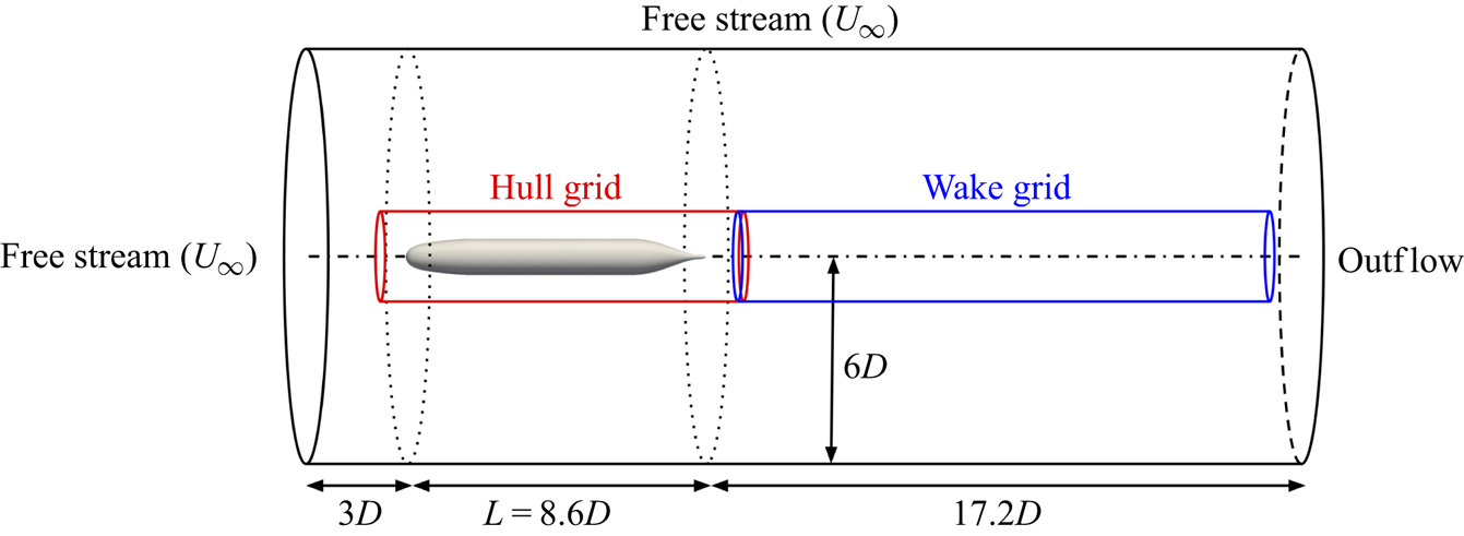
Figure 3. Computational domain for simulation of the bare DARPA SUBOFF hull. The outer boundary of the hull grid is shown in red and the wake refinement grid boundary is in blue. The outer boundary of the background grid is in black, where boundary conditions are labelled.
The experiments of Jiménez, Hultmark & Smits (Reference Jiménez, Hultmark and Smits2010b) for the bare SUBOFF hull at the same Reynolds number employed a trip wire of diameter 0.005 $D$ located a distance $x/D = 0.75$ from the nose to promote transition of the boundary layer. To replicate the experimental conditions, the boundary layer is tripped in the computations at the same axial location by applying a steady wall-normal velocity of $0.06U_{\infty }$ at this $x$-location. The motivation behind this tripping method is to lift the boundary layer to mimic the effect of a trip wire, and has been shown to promote quick transition of the flow (Kumar & Mahesh Reference Kumar and Mahesh2018b). The local effect of the trip will be further discussed in the present work in terms of the streamline curvatures induced by the wall-normal blowing.
The present computations are performed on three separate overset grids, as shown in figure 3. A cylindrical grid attached to the hull extends from  $1.2D$ in front of the nose to $1.62D$ downstream of the end of the hull with a radius of $1.2D$. A second grid with the same radius extends from the end of the hull grid to $x/D = 25.2$ to refine the wake behind the body. A final ‘background’ grid envelopes the two overset grids and extends to the boundaries of the computational domain to supply the far-field and outflow boundary conditions. This background grid is stretched in the $r$-direction and coarsened by a factor of 1.5 in the $x$- and $\theta$-directions relative to the hull and wake grids to reduce the computational cost. The summary of the number of cells and processors for each grid is given in table 2. The final computation was performed with a total of 712 million control volumes partitioned over 9504 processors. The simulation is performed with a time step of ${\rm \Delta} t U_{\infty }/D = 0.0012$ for two flow-through times ( $t = 57.6D/U_{\infty }$) to discard initial transients and for another two flow-through times to collect statistics.
Table 2. Details of the three grids, including the number of control volumes and the number of processors per grid.
4. Results and discussion
The bare SUBOFF hull geometry provides an ideal test case to examine the properties of equations in the streamline coordinate system. In this section, we will first examine the flow field globally in § 4.1, followed by comparison to experiments in § 4.2. In § 4.3, we describe the integral development of the hull boundary layer before examining the pressure variation within the boundary layer using streamline boundary layer equations in § 4.4. The stagnation point flow and curved laminar boundary layer over the front of the hull are discussed in § 4.5. In this area of the flow, the turbulence terms drop out of the boundary layer momentum equations. We follow by discussing the zero-pressure-gradient turbulent boundary layer (ZPGTBL) over the parallel mid-hull in § 4.6, where the curvature and streamwise pressure gradient terms drop out of the momentum equations. Finally, the thick stern boundary layer is analysed in §§ 4.7–4.10. Both the curvature and turbulence terms appear in the equations for the stern boundary layer, emphasizing the complexity of the flow.
4.1. Overview of the flow field
Figure 4 shows an isocontour of instantaneous  $Q$-criterion (Hunt, Wray & Moin Reference Hunt, Wray and Moin1988) coloured by the instantaneous axial velocity to show the turbulent structures near the wall. The flow is verified to quickly transition after the tripping location at $x/D = 0.75$. The fine azimuthal resolution is required to capture the streaky flow structures visible in the boundary layer over the mid-hull. Figure 5 shows contours of the circumferentially averaged eddy viscosity normalized by the molecular viscosity around the hull. The magnitude of the eddy viscosity is low in the boundary layer, suggesting that the flow is being resolved adequately. Subsequent comparison with experimental measurements (§ 4.2) will further confirm the reliability of the simulation.
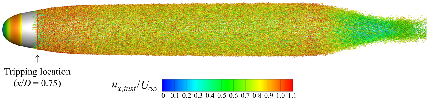
Figure 4. Instantaneous isocontour of  $Q$-criterion (Hunt et al. Reference Hunt, Wray and Moin1988) coloured by instantaneous axial velocity are shown near the hull surface to visualize near-wall structures. The transition of the boundary layer is visible at the tripping location ( $x/D = 0.75$).
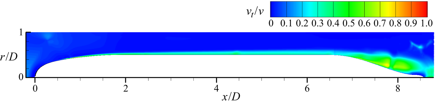
Figure 5. Circumferentially averaged mean eddy viscosity normalized by the molecular viscosity around the hull.
Contour plots of the instantaneous velocity and vorticity magnitudes, the average streamwise velocity ( $U_s$) and the pressure coefficient are shown in figure 6. The pressure coefficient is defined as
 \begin{equation} C_p = \frac{P - P_{\infty}}{\frac{1}{2}\rho U_{\infty}^{2}} , \end{equation}
where  $P_{\infty }$ and $U_{\infty }$ are the reference pressure and free-stream velocity. Also shown in each contour is a black line representing the edge of the boundary layer/wake. The traditional definition of the boundary layer edge ( $0.995 U_{\infty }$) is not adequate for this flow since the velocity varies outside of the boundary layer due to streamwise pressure gradients and streamline curvature. Therefore, an alternative definition is required. Several general methods of calculating the boundary layer thickness have been suggested, from definitions based on vorticity (Spalart & Watmuff Reference Spalart and Watmuff1993; Coleman, Rumsey & Spalart Reference Coleman, Rumsey and Spalart2018) to methods based on the total pressure (Patel et al. Reference Patel, Nakayama and Damian1974; Griffin, Fu & Moin Reference Griffin, Fu and Moin2021). In this work, we use the $0.99 C_{p_{tot},\infty }$ total pressure metric used by Patel et al. (Reference Patel, Nakayama and Damian1974). This total pressure definition reduces to the usual $0.995U_{\infty }$ definition on the mid-hull where there are minimal pressure variations across the boundary layer.
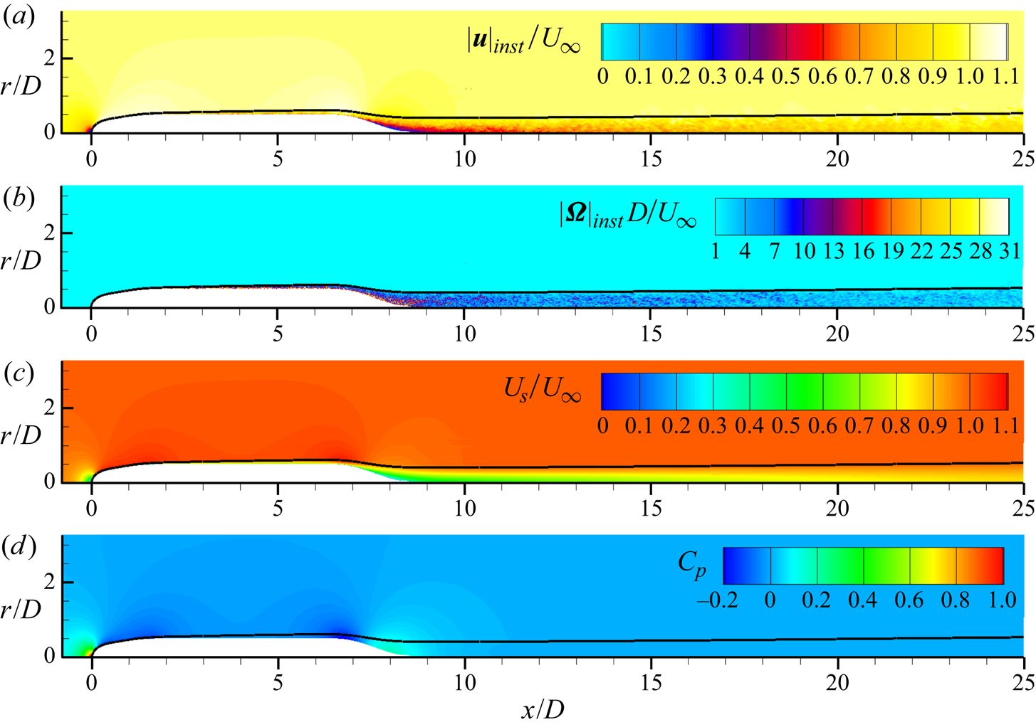
Figure 6. Contours of (a) instantaneous velocity magnitude, (b) instantaneous vorticity magnitude, (c) mean streamwise velocity and (d) mean pressure coefficient. The black line designates the edge of the boundary layer and wake using the total pressure metric.
The boundary layer is relatively thin over most of the hull, but its growing thickness is apparent in figure 6 even before the stern starts to taper. The boundary layer grows rapidly over the stern, the thickness quickly becoming much larger than the local radius of the hull, followed by the slow spreading of the intermediate wake.
4.2. Hull surface stresses and comparison to experiments
The pressure and skin friction coefficients on the hull are compared to the experimental data of Huang et al. (Reference Huang, Liu, Groves, Forlini, Blanton and Gowing1992) in figure 7. The skin friction coefficient is defined as
 \begin{equation} C_f = \frac{\tau_w}{\frac{1}{2} \rho U_{\infty}^{2}}, \end{equation}
where  $\tau _w$ is the shear stress at the wall. Note that the experimental measurements were conducted at $Re_L = 1.2 \times 10^{7}$ as opposed to the present $Re_L = 1.1 \times 10^{6}$, but are used for comparison due to the lack of surface measurements for the present Reynolds number ( $Re$).

Figure 7. Profiles of (a)  $C_p$ and (b) $C_f$ on the hull surface: ——, hull surface quantities; $\cdot \cdot \cdot \cdot \cdot \cdot$, $C_p$ along boundary layer edge; $\square$, experiments of Huang et al. (Reference Huang, Liu, Groves, Forlini, Blanton and Gowing1992) at $Re = 1.2 \times 10^{7}$; – – – – (red), flat-plate ZPGTBL $C_f$ curve from Schlichting (Reference Schlichting1955). Note that the experimental $C_f$ data have been scaled to the $Re$ of the simulation using the scaling $C_f \sim Re^{-1/5}$.
Since  $C_p$ is fairly insensitive to $Re$ for high $Re$, the experimental surface pressure data are compared directly to the present results. The agreement between the LES and the experimental data is good. Note that the spike in the numerical $C_p$ curve at $x/D = 0.75$ corresponds to the tripping location. Over the stern, the adverse pressure gradient imposed by the hull geometry causes the boundary layer to thicken rapidly, and the thickness of the resulting stern boundary layer is determined by the Reynolds number. The thicker boundary layer at the lower $Re$ of the present simulations decreases the streamline curvature over the stern, resulting in lower peaks in $C_p$ at $x/L = 0.78$ and $x/L = 0.94$ compared to the experimental measurements. Also shown in figure 7 is the pressure coefficient plotted along the edge of the boundary layer. The hull surface pressure and the edge pressure are similar for $0 < x/L < 0.7$, despite small differences at the pressure dip after the tripping location. However, the two pressures rapidly diverge after $x/L = 0.7$ as the stern boundary layer thickens, changing the streamline curvature across the boundary layer. The result is that fluid near the edge of the boundary layer experiences significantly smaller pressure gradients compared to flow near the wall. Clearly the streamwise pressure gradient at the wall does not describe the pressure gradient across the rest of the boundary layer at the stern.
To compare the skin friction coefficient to Huang et al. (Reference Huang, Liu, Groves, Forlini, Blanton and Gowing1992), we apply  $C_f \sim Re^{-1/5}$ scaling for high- $Re$ attached ZPG boundary layers to scale the experimental data to the present $Re$. While this scaling is valid only for the mid-section of the hull, we see good agreement between the present results and the experimental data. For additional comparison, figure 7 also shows the analytical $C_f$ curve for a flat-plate ZPGTBL, detailed by Schlichting (Reference Schlichting1955) as
 \begin{equation} C_f = 0.0576 ( Re_x ) ^{-{1}/{5}} = 0.0576 \left(\frac{U_{\infty} ( x - x_t )}{\nu}\right)^{-{1}/{5}} , \end{equation}
where we choose the location of the trip,  $x_t$, as the virtual origin. The agreement with the analytical $C_f$ curve is good over the ZPG region of the hull that is not affected by the influence of the hull's longitudinal curvature. The analytical relation for a flat-plate ZPGTBL is suitable for comparison to the present axisymmetric TBL since the ratio of the boundary layer thickness to the local transverse curvature is small over the mid-section of the hull.
Additional comparison is made to experimental measurements by Jiménez et al. (Reference Jiménez, Hultmark and Smits2010b) on the unappended SUBOFF hull at  $Re_L = 1.1 \times 10^{6}$. The drag coefficient is defined as
 \begin{equation} C_D = \frac{F_D}{\frac{1}{2} \rho U_{\infty}^{2} S}, \end{equation}
where  $F_D$ is the drag force and $S = {\rm \pi}D^{2}/{4}$ is the projected area of the hull. Jiménez et al. (Reference Jiménez, Hultmark and Smits2010b) estimated a drag coefficient of 0.136 by integrating an exponential function fitted to the mean velocity measurements in the wake on the opposite side of the experimental support. Note that the model in the experiments was supported by a semi-infinite sail that was found to affect the lower half of the wake (Jiménez et al. Reference Jiménez, Hultmark and Smits2010b). The drag coefficient calculated using the total hull drag for the present computations is 0.143.
Figure 8 shows comparison of the mean streamwise velocity to the measurements of Jiménez et al. (Reference Jiménez, Hultmark and Smits2010b) on the side opposite to the support at  $x/D = 3, 6, 9, 12, 15$ downstream of the stern. At all stations, there is good agreement between the present results and the experiments. The ratio of the model diameter to the wind tunnel diameter in the experiments was 20.8 %, leading to a blockage of 4.3 % due to the model alone. Combined with the support, the total blockage in the experiments was 5.7 %, compared to the 0.7 % blockage of the present computations. This may affect the wake width and centreline velocity deficit of the experiments in comparison to the present computation, even given the similar drag value.
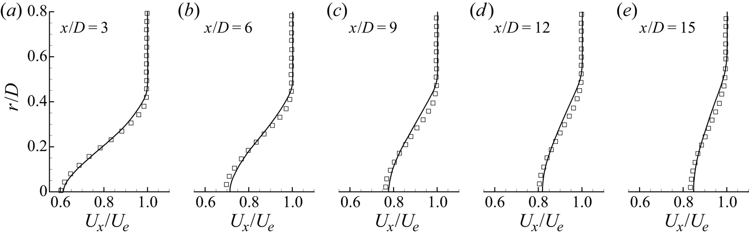
Figure 8. Profiles of mean axial velocity normalized by edge velocity at stations  $x/D = 3, 6, 9, 12, 15$ downstream of the stern: ——, present results; $\square$, experiments of Jiménez et al. (Reference Jiménez, Hultmark and Smits2010b).
4.3. Hull boundary layer development
Figure 9 shows the development of the hull boundary layer in terms of the boundary layer thickness ( $\delta$), the shape factor ( $H$), the momentum-thickness Reynolds number ( $Re_{\theta }$), the friction Reynolds number ( $Re_{\tau }$) and the Clauser pressure gradient parameter ( $\beta$). Note that $H = \delta ^{*}/\theta$, $Re_{\tau } = \delta u_{\tau } / \nu$, $Re_{\theta } = \theta U_{\infty } / \nu$ and $\beta = \delta ^{*}/\tau _w \partial P/\partial s$, where $u_{\tau } = \sqrt {\tau _w/\rho }$ is the friction velocity. The displacement thickness, $\delta ^{*}$, and the momentum thickness, $\theta$, are calculated in the streamwise-normal direction using the usual axisymmetric definitions as
 \begin{equation} \delta^{*} = \int_0^{\delta}\left(1-\frac{U_s}{U_e}\right)\frac{r}{a}\,\textrm{d}n, \quad \theta = \int_0^{\delta} \frac{U_s}{U_e} \left( 1 - \frac{U_s}{U_e} \right) \frac{r}{a} \, \textrm{d}n, \end{equation}
where  $U_e$ is the velocity at the edge of the boundary layer and $a$ is the local radius of the hull. Note that the values of $\delta ^{*}$ and $\theta$ may be sensitive to the definition of the boundary layer thickness. To investigate this sensitivity, we compare the total pressure definition of $\delta$ from Patel et al. (Reference Patel, Nakayama and Damian1974) to the inviscid reconstruction method proposed by Griffin et al. (Reference Griffin, Fu and Moin2021) in figure 9(a). The method of Griffin et al. (Reference Griffin, Fu and Moin2021) constructs an inviscid velocity $U_i$ using the Bernoulli equation, which is used to define $\delta$ as the point where the velocity in the boundary layer reaches $0.995 U_i$. Figure 9(a) shows that the two methods produce nearly identical values of $\delta$ over the length of the hull, providing confidence that the calculations of $\delta ^{*}$ and $\theta$ are not sensitive to these choices of $\delta$. Therefore, in the remainder of the paper, we retain the total pressure metric of Patel et al. (Reference Patel, Nakayama and Damian1974) as the definition of the boundary layer edge.
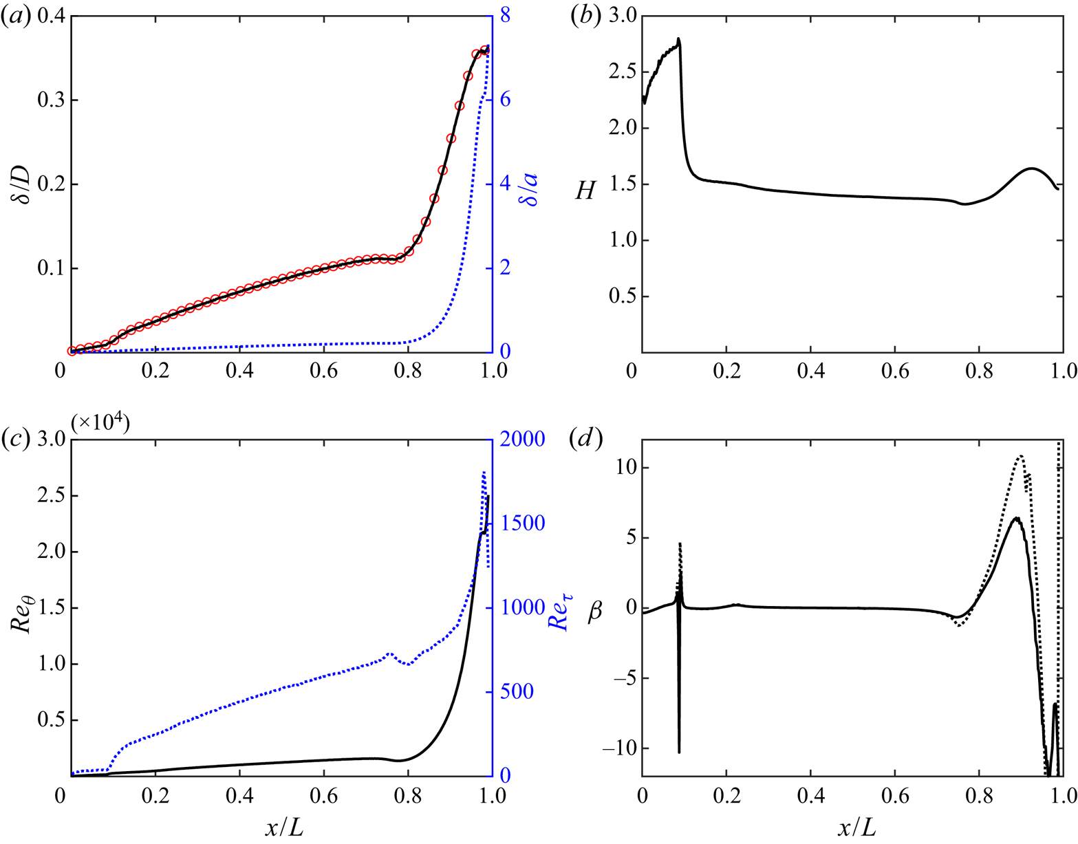
Figure 9. Variation of (a) boundary layer thickness, (b) shape factor, (c)  $Re_{\theta }$ and $Re_{\tau }$, and (d) the boundary layer edge (——) and wall ( $\cdot \cdot \cdot \cdot \cdot \cdot$) Clauser pressure gradient parameters versus $x/L$ along the hull. Profiles are extracted along the streamline-normal coordinate direction from lines originating at the hull surface. The red symbols in panel (a) represent $\delta /D$ at intervals along the hull computed using the inviscid velocity method of Griffin et al. (Reference Griffin, Fu and Moin2021).
Examining figure 9, boundary layer thickness increases along the mid-section of the hull followed by a dip at  $x/L \approx 0.8$ where the mild favourable pressure gradient causes a thinning of the boundary layer. Following this region, the boundary layer thickens rapidly, quickly approaching 35 % of the hull diameter. This rapid increase in thickness, combined with the tapering of the hull, causes $\delta /a$ to increase from 0.22 at the end of the parallel mid-hull to over 6 by the end of the stern. The evolution of $H$ in figure 9(b) clearly shows the effect of the trip, where $H$ quickly transitions from values typical of laminar boundary layers to that of turbulent boundary layers. Note that the value of $H=2.59$ for the Blasius boundary layer is not realized over the front of the hull due to the presence of favourable and adverse pressure gradients before the trip location. Over the stern the shape factor increases along with the adverse pressure gradient, followed by a small decrease in the favourable-pressure-gradient region near the end of the body.
In the definition of  $\beta$, $\partial P / \partial s$ is the pressure gradient, which is typically evaluated along the boundary layer edge. In figure 9(d), we plot this traditional definition along with $\beta$ evaluated with the pressure gradient along the wall. For flows without curvature, these two definitions would be equal since the wall pressure is equal to the free-stream pressure using the typical boundary layer equations. However, in the presence of non-negligible streamline curvature, this simplification breaks down. Over the front of the body, there is significant curvature, but the laminar boundary is thin enough that the accumulated effect of the streamline curvature does not cause significant deviations of the wall pressure gradient from the pressure gradient at the boundary layer edge. However, as the boundary layer thickens, this effect becomes more significant and the wall feels a much stronger adverse pressure gradient than the boundary layer edge for $0.81 < x/L < 0.94$. Past $x/L = 0.94$, the pressure gradients at the wall and boundary layer edge are completely uncorrelated, as the near-wall flow feels a strong switch between favourable and adverse pressure gradients over the curved tip of the stern, leading to separation for $x/L > 0.99$. At the same location, the boundary layer edge responds only to the favourable pressure gradient of the external flow.
4.4. Streamline boundary layer equations and pressure variation in the boundary layer
Insight into the behaviour of the pressure gradients throughout the boundary layer can be developed by considering the boundary layer approximations of the streamline and streamline-normal momentum equations:
 \begin{equation} \left.\begin{gathered} U_s \frac{\partial U_s}{\partial s} ={-}\frac{1}{\rho} \frac{\partial P}{\partial s} - \frac{1}{r} \frac{\partial}{\partial n} \left( r \overline{u_s u_n} - r \nu \frac{\partial U_s}{\partial n} \right) , \\ \frac{U_s^{2}}{R_s} ={-}\frac{1}{\rho} \frac{\partial P}{\partial n} - \frac{1}{r} \frac{\partial}{\partial n} \left( r \overline{u_n^{2}} \right), \end{gathered}\right\} \end{equation}
where we have retained only the leading-order terms. The magnitudes of the other terms in (2.23) and (2.28) will be evaluated in the discussion of flow over the stern.
The equations are quite similar to the axisymmetric boundary layer equations and are easily simplified to the two-dimensional boundary layer equations by separation and removal of the terms containing  $r$. The differences between the present equations and the traditional boundary layer equations are the simplification of the advection term on the left-hand side of the streamwise momentum equation and the addition of the $U_s^{2}/R_s$ term in the streamwise-normal momentum equation. This additional term is the source of the variation in pressure across the boundary layer on the curved stern. Integration of this second equation in the streamline-normal direction followed by differentiation in $s$ yields
 \begin{equation} \frac{1}{\rho} \frac{\partial P}{\partial s} = \frac{1}{\rho} \frac{\partial P_w}{\partial s} - \frac{\partial \overline{u_n^{2}}}{\partial s} - \frac{\partial}{\partial s} \int_0^{n} \overline{u_n^{2}} \frac{1}{r} \frac{\partial r}{\partial n'} \, \textrm{d}n' - \frac{\partial}{\partial s} \int_0^{n} \frac{U_s^{2}}{R_s} \, \textrm{d}n', \end{equation}
where  $P_w$ is the pressure at the wall, $n'$ is the integration variable for the streamline-normal distance, and we will subsequently neglect the terms containing the streamwise derivative of $\overline {u_n^{2}}$. We can see that the integrated effect of the $U_s^{2}/R_s$ term governs the difference between the streamwise pressure gradient at the wall and the pressure gradient at any other point in the streamwise-normal direction.
Further insight is obtained by splitting  $1/R_s$ into its components using (2.25), producing
 \begin{equation} \frac{1}{\rho} \frac{\partial P}{\partial s} + U_s \frac{\partial U_s}{\partial s} = \frac{1}{\rho} \frac{\partial P_w}{\partial s} - \frac{\partial}{\partial s} \int_0^{n} U_s \varOmega \,\textrm{d}n' , \end{equation}
where we note that the streamwise derivative cannot be moved into the integral without application of the full form of the Leibniz integral rule, which problematically reintroduces the integrating factor  $\zeta$.
The first result of (4.8) is obtained by choosing  $n \geqslant \delta$. Since we know from (2.23) that the terms on the left-hand side of (4.8) sum to zero outside of the boundary layer, choosing $n = \delta$ yields
 \begin{equation} P_w - P_e = \tfrac{1}{2} \rho U_e^{2} + \rho \int_0^{\delta} U_s \varOmega \,\textrm{d}n', \end{equation}
where  $P_e$ and $U_e$ are the pressure and velocity at the edge of the boundary layer. Note that this expression may be reformulated with the choice of any $n \geqslant \delta$ as the integration maxima (with corresponding values of $P_e$ and $U_e$), as long as the gradients of the viscous and turbulent stresses are negligible at this point. For boundary layers with negligible curvature, $\varOmega \simeq \varOmega _{shear} = - \partial U_s / \partial n$, and the integral term on the right-hand side reduces to $- \rho U_e^{2}/{2}$, recovering $P_w = P_e$ from the typical boundary layer equations. It is therefore apparent that the rotational vorticity is the component that contributes to the pressure variation in the boundary layer, as this term is associated with the streamline curvature. Rewriting (4.9) in terms of the pressure coefficient at the wall, we find
 \begin{equation} C_p = 1 + \frac{2}{U_{\infty}^{2}} \int_0^{\infty} U_s \varOmega \,\textrm{d}n', \end{equation}
where we note that the integral of  $U_s \varOmega$ converges outside of the boundary layer.
Figure 10(a) shows a comparison of the left-hand and right-hand sides of (4.9) non-dimensionalized by  $\rho U_{\infty }^{2}/{2}$. As expected, $P_w = P_e$ over the parallel mid-section of the hull, but diverges for the curved flow around front and stern. The greater difference in the pressures at the stern compared to the front of the hull is due to the thicker boundary layer, which leads to a larger integral of $U_s \varOmega$ given the streamline curvature in the boundary layer. The match between the sides of the equation is excellent over most of the hull. Figure 10(b) shows the pressure coefficient measured at the wall versus the right-hand side of (4.10) evaluated by integrating along streamline-normal lines emanating from the hull surface. Again, the agreement is excellent even around the trip location and at the very tip of the stern.
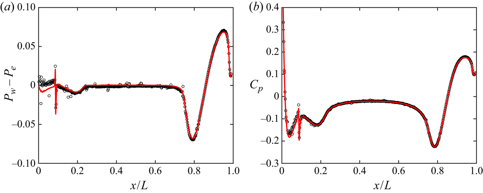
Figure 10. (a) Left-hand (——) and right-hand ( $\circ$) sides of (4.9) non-dimensionalized by $\rho U_{\infty }^{2}/{2}$, representing the difference between pressures at the wall and the edge of the boundary layer. (b) Pressure coefficient measured at the wall (——) compared to the right-hand side of (4.10) ( $\circ$).
A second result is obtained by substituting the result of (4.8) into (4.6) to produce
 \begin{equation} \frac{\partial}{\partial s} \left[ \frac{P_w}{\rho} - \int_0^{n} U_s \varOmega \,\textrm{d}n' \right] = \frac{1}{r} \frac{\partial}{\partial n} \left[ r \nu \frac{\partial U_s}{\partial n} - r \overline{u_s u_n} \right]. \end{equation}
This equation can be written in alternative form as
 \begin{equation} \frac{\partial}{\partial s} \int_n^{\infty} U_s \varOmega \,\textrm{d}n' = \frac{1}{r} \frac{\partial}{\partial n} \left[ r \nu \frac{\partial U_s}{\partial n} - r \overline{u_s u_n} \right]. \end{equation}
The bracketed term on the right-hand side is recognizable as the total stress, and the pressure gradient and advection terms from the original boundary layer equation have been replaced by the term on the left-hand side. These equations can be considered the form of the boundary layer momentum equation for general boundary layers along curved walls.
4.5. Front of the hull: stagnation point, laminar boundary layer and trip flow
Figure 11 shows contours of  $U_s$ and $C_p$, as well as non-dimensional curvatures $D/R_s$ and $D/L_a$, for flow over the front of the hull. The flow approaching the front of the hull experiences a strong adverse pressure gradient ahead of the stagnation point, causing the streamlines to curve significantly as the flow follows the contour of the body. The deceleration of the flow near the stagnation point and the following acceleration about the bow are reflected by the contour of $D/L_a$, which represents the inverse of the streamwise acceleration length scale. The changing distance between adjacent streamlines at the bow visually reflects the acceleration of the flow.
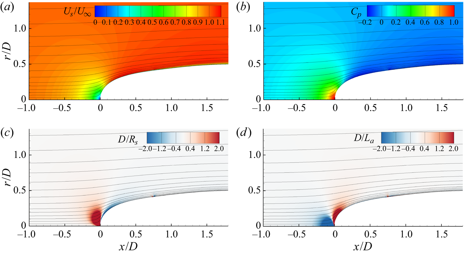
Figure 11. Contours of (a)  $U_s/U_{\infty }$, (b) $C_p$, (c) $D/R_s$ and (d) $D/L_a$ along with streamlines over the front of the hull.
Along with the streamline accelerations, figure 11 also shows the streamline curvature, which quickly switches signs from the stagnation point flow to the streamlines following the contour of the bow. This curvature is much stronger than at any other point in the flow field, but the strongest effects near the stagnation point are limited to the potential flow outside of the boundary layer. However, for cases with free-stream turbulence or bodies immersed in turbulent flow, there may be significant distortion of the incoming turbulence due to this curvature. Muck, Hoffmann & Bradshaw (Reference Muck, Hoffmann and Bradshaw1985) and Hoffmann, Muck & Bradshaw (Reference Hoffmann, Muck and Bradshaw1985) concluded that turbulence is amplified by concave curvature and attenuated by convex curvature, and that the lateral divergence in combination with the convex curvature near the stagnation point serves to amplify turbulence (Smits et al. Reference Smits, Eaton and Bradshaw1979a). This behaviour was observed by Ding et al. (Reference Ding, Saxton-Fox, Hultmark and Smits2019) for an axisymmetric body in a turbulent pipe flow. This indicates that incoming turbulence in closest contact with the boundary layer on streamlined bodies may be significantly altered by the curvature of the streamlines near the stagnation point.
Also visible in the contours of  $D/R_s$ and $D/L_a$ is the effect of the trip at $x/D = 0.75$, which locally produces strong upward and downward curvature of the streamlines along with alternating streamwise decelerations and accelerations. This behaviour appears to mimic the expected behaviour of streamlines over a physical trip wire, indicating that the numerical blowing trip produces effects similar to that of a solid trip wire.
Figure 12 shows contours of the rotational and shear components of vorticity from (2.26) along with the total mean vorticity around the front of the hull. Around the stagnation point, the streamline curvature produces a large amount of rotational vorticity, but this component is cancelled by the shear vorticity to produce zero net vorticity. This is required for potential flow by the vorticity equation for initially irrotational flow without viscous effects. Inside the boundary layer, however, the shear vorticity generated by the viscous stress at the wall dominates the rotational vorticity, and by the time the flow reaches the parallel mid-section of the hull the rotational vorticity in the boundary layer is negligible.
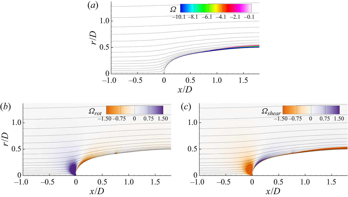
Figure 12. Contours of (a) total vorticity ( $\varOmega$), (b) rotational vorticity ( $\varOmega _{rot} = U_s/R_s$) and ( $c$) shear vorticity ( $\varOmega _{shear} = -\partial U_s / \partial n$) non-dimensionalized by $D/U_{\infty }$ along with streamlines over the front of the hull.
Figure 13 shows profiles of streamwise velocity and rotational vorticity along potential (streamwise-normal) lines originating from the hull surface. The benefits of the streamline coordinate system are clear in figure 13(a), as the potential lines are normal to the hull surface as they approach the wall and are normal to the free-stream velocity vector far from the hull surface. It is clear also that the alternative metric to identify the boundary layer edge is required since the velocity at the edge of the boundary layer varies from less than half of the free-stream value near the stagnation point to nearly 10 % over the free-stream velocity further along the bow. The rotational vorticity is strongest near the stagnation point, where it actually switches signs outside of the boundary layer. The rotational vorticity in the boundary layer increases away from the wall to values that represent the changing curvature and increasing velocity profile throughout the boundary layer profile. Since the rotational vorticity is zero by definition at the wall, we see that the shear vorticity is the sole link between the vorticity and viscous stress at the wall. Although the shear vorticity dominates in the boundary layer, the rotational vorticity remains important, as it dictates the variation of pressure in the boundary layer, especially for flow over the stern.
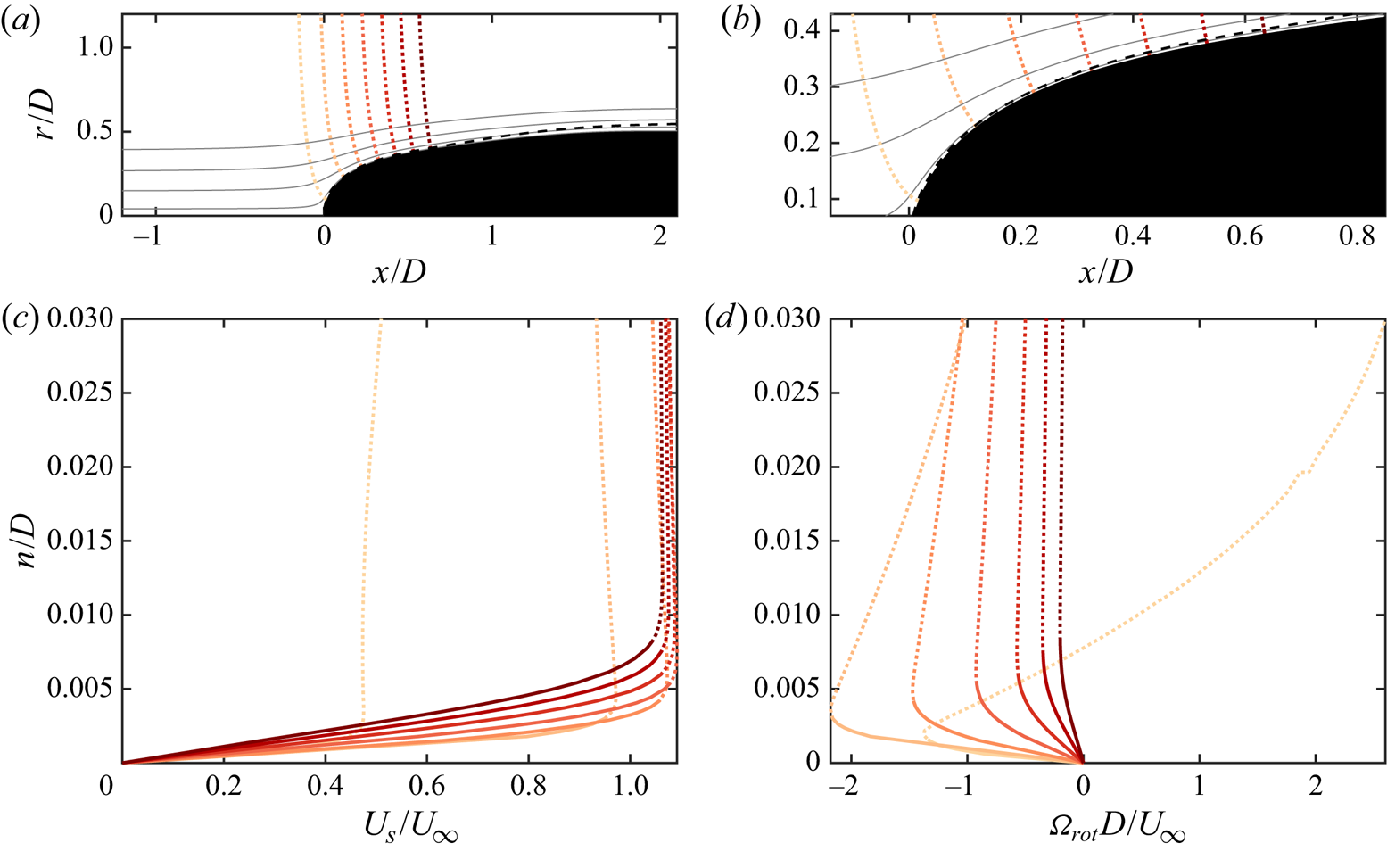
Figure 13. Streamline-normal lines (shades of red) along with boundary layer edge (black – – – –) and streamlines (grey) on the front of the hull (a) and zoomed in near the wall (b). Corresponding profiles of (c) mean streamwise velocity and (d) rotational vorticity, where dotted lines indicate locations outside of the boundary layer.
Figure 14 shows the terms in the streamwise and streamwise-normal momentum equations (4.6) for the third potential line from figure 13(a). Since there is no turbulence before the tripping location, the streamwise momentum equation is a simple balance between the mean advection, pressure gradient and viscous forces. Outside of the boundary layer, the viscous term goes to zero and the pressure gradient exactly balances the mean advection along the streamlines, following the differential form of Bernoulli's equation. Examining the streamline-normal momentum equation, the lack of turbulence in the laminar boundary layer means that this equation represents an equivalence between the streamline-normal pressure gradient and the centripetal acceleration of the fluid elements along the streamline path ( $U_s^{2}/R_s$). The advantages of streamline coordinate analysis are immediately apparent even for this relatively simple region of the flow. The streamline and streamline-normal momentum balances intuitively explain the balance of centripetal acceleration, advection, pressure gradients and viscous forces in the boundary layer while naturally reducing to the differential Bernoulli equation and the $s$–
$s$– $n$ Euler equation where viscous effects are negligible.
Figure 14. Profiles of the terms in the mean momentum equations for the third potential line in figure 13(a). (a) Terms in the streamwise momentum equation:  $U_s ({\partial U_s}/{\partial s})$ (blue), $-({1}/{\rho })({\partial P}/{\partial s})$ (red) and $({1}/{r})({\partial }/{\partial n} )( r \nu ({\partial U_s}/{\partial n} ))$ (brown). (b) Terms in the streamwise-normal momentum equation: ${U_s^{2}}/{R_s}$ (blue) and $-({1}/{\rho } )({\partial P}/{\partial n})$ (red). All terms are non-dimensionalized using inner scales ( $\nu /u_{\tau }^{3}$). Dotted lines represent points outside of the boundary layer using the total pressure metric.
4.6. ZPGTBL on the parallel mid-hull
The geometry of the SUBOFF hull has a parallel mid-section from  $x/L = 0.23$ to $x/L = 0.74$, where $a = R = {D}/{2}$. While the start and end of this section are affected by the preceding and following pressure gradients, the flow is nominally a ZPG axisymmetric boundary layer over this region. Figure 15 shows profiles of inner-scaled mean velocity and root-mean-square (r.m.s.) turbulence intensities for potential lines originating at the hull surface for $2.4 < x/D < 6$. The potential lines are nearly vertical since the axial velocity is much larger than the radial velocity over the mid-section. Also shown in the figure are direct numerical simulation (DNS) results for a planar TBL ( $Re_{\theta } = 1551$, $Re_{\tau } = 578$) by Jiménez et al. (Reference Jiménez, Hoyas, Simens and Mizuno2010a), which are at a comparable Reynolds number to the last potential line profile on the mid-hull ( $Re_{\theta } = 1446$, $Re_{\tau } = 660$). The higher $Re_{\tau }$ for the hull boundary layer compared to the flat plate at similar $Re_{\theta }$ can be attributed to the higher skin friction coefficients observed for axisymmetric TBLs compared to their planar counterparts (Piquet & Patel Reference Piquet and Patel1999; Kumar & Mahesh Reference Kumar and Mahesh2018a). The fact that the axial velocity is much greater than the radial velocity ( $U_x \gg U_r$) over the mid-hull means that the differences are very small between streamline coordinate measurements and measurements in a Cartesian/cylindrical frame. Rotating the measurements from the Cartesian frame to the streamline frame produces a nearly imperceptible shift in the profiles, demonstrating that results of flat-plate boundary layer analysis for the law of the wall and the laminar sublayer are still applicable in streamline coordinates.
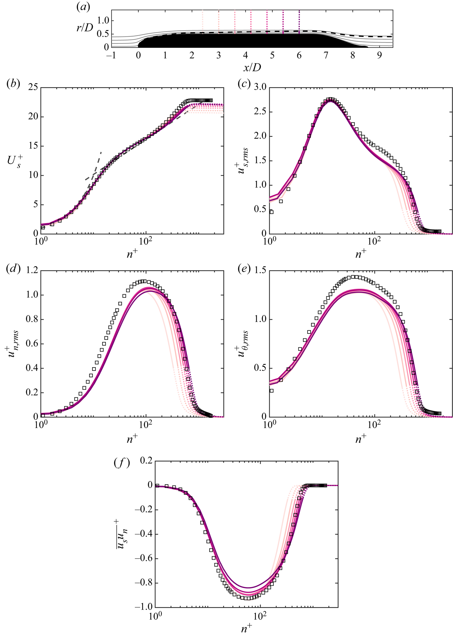
Figure 15. Streamline-normal lines (shades of magenta) on the mid-hull originating from the hull surface at  $x/D = 2.4$, 3.0, 3.6, 4.2, 4.8, 5.4, 6.0, along with boundary layer edge (black – – – –) using the total pressure metric (a). Note that the streamline-normal profiles are nearly vertical since $U_x \gg U_r$ over the mid-hull. Associated profiles of inner-scaled mean streamwise velocity (b) and streamwise (c), streamwise-normal (d) and $\theta$-direction (e) velocity fluctuations along with Reynolds shear stress (f) are compared to the DNS results of Jiménez et al. (Reference Jiménez, Hoyas, Simens and Mizuno2010a) for a planar TBL at $Re_{\theta } = 1551$. Velocity profiles for the log law and viscous sublayer (grey – – – –) are also shown in panel (b). Points outside of the boundary layer (based on the total pressure metric) are dotted lines.
Figure 16 shows the terms from the streamwise and streamwise-normal equations (4.6) for the fourth potential line in figure 15(a) emanating from the hull surface at  $x/D = 4.2$. In contrast to the curved laminar boundary layer driven by a pressure gradient in figure 14, the boundary layer at this location on the mid-hull has a negligible streamwise pressure gradient and nearly zero streamline curvature. This is evidenced by the near-zero values of $-({1}/{\rho } )({\partial P}/{\partial s})$ and $U_s^{2}/R_s$ in figure 16(a,b). However, as opposed to the laminar boundary layer at the front of the hull, the fully developed TBL over the mid-hull produces Reynolds stresses that dominate the budgets inside the boundary layer. In the streamwise momentum equation, the Reynolds shear stress gradient and the viscous term cancel each other in the viscous sublayer before the viscous term loses leading-order dominance by the start of the log layer. From the start of the log layer to the edge of the boundary layer, the advection of the streamwise velocity follows the gradient of $\overline {u_s u_n}$.
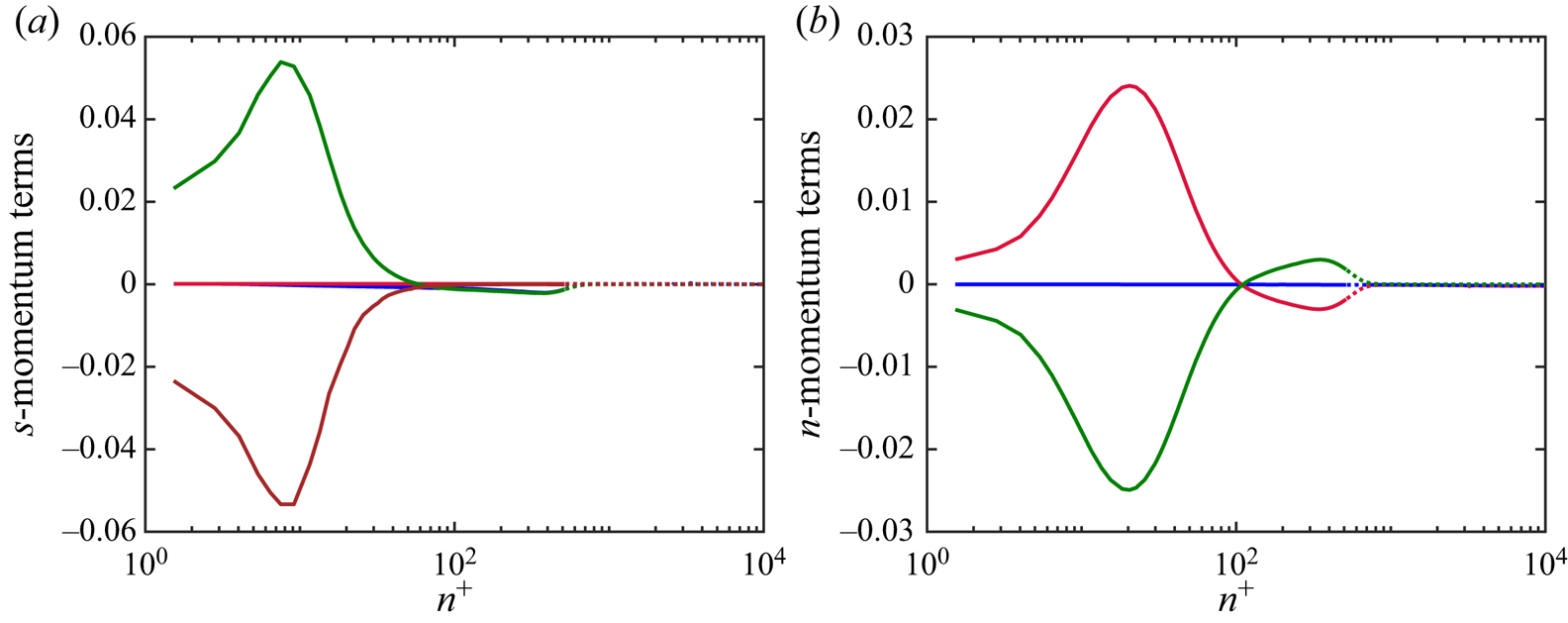
Figure 16. Profiles of terms in the boundary layer equations for the streamline-normal line emanating from  $x/D = 4.2$ on the hull surface (the fourth line from figure 15a). (a) Terms in the streamwise momentum equation: $U_s ({\partial U_s}/{\partial s})$ (blue), $-({1}/{\rho } )({\partial P}/{\partial s})$ (red), $-({1}/{r})({\partial }/{\partial n} )( r \overline {u_s u_n} )$ (green) and $({1}/{r})({\partial }/{\partial n}) ( r \nu ({\partial U_s}/{\partial n} ))$ (brown). ( $b$) Terms in the streamwise-normal momentum equation: ${U_s^{2}}/{R_s}$ (blue), $-({1}/{\rho } )({\partial P}/{\partial n})$ (red) and $-({1}/{r})( {\partial }/{\partial n} )( r \overline {u_n^{2}} )$ (green). All terms are non-dimensionalized using inner scales ( $\nu /u_{\tau }^{3}$). Dotted lines represent points outside of the boundary layer.
In general, the mean advection term is much smaller than for the laminar profile due to the lack of streamwise pressure gradients over the mid-hull. This mean advection term also returns to zero outside of the boundary layer, which is not the case for pressure gradient flows. Examination of the terms in the streamwise-normal momentum equation (figure 16b) reveals that the streamwise-normal pressure gradient balances the streamwise-normal gradient of  $\overline {u_n^{2}}$, as typical for planar TBLs. The result is that the pressure at the wall is equal to the pressure outside of the boundary layer, as observed in figure 10(a). Overall, the budgets of streamwise and streamwise-normal mean momentum are consistent with the classical interpretation of ZPG boundary layer structure.
4.7. Overview of the thick stern boundary layer
As discussed previously, the boundary layer approaching the stern begins at a thickness of slightly over 20 % of the local hull radius and quickly increases to over six times the local radius by the end of the stern. Figure 17 shows contours of streamline coordinate variables for the flow field at the stern.
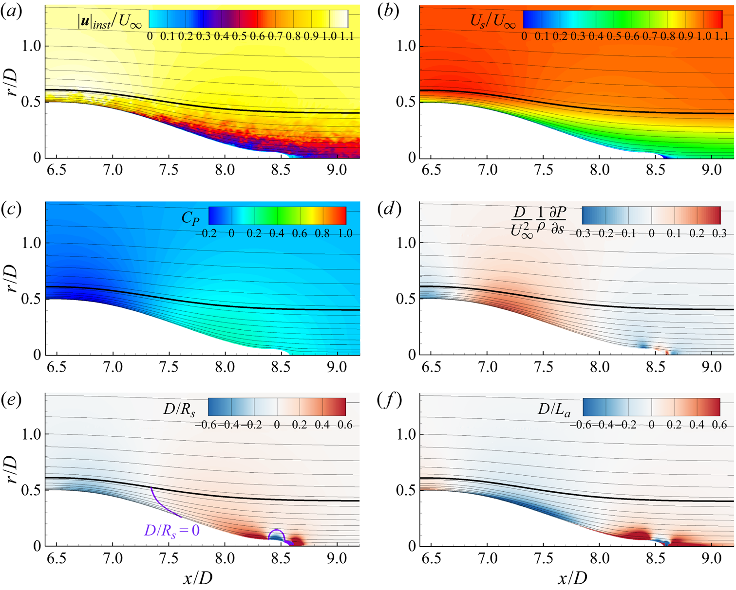
Figure 17. Contours of (a) instantaneous velocity magnitude, (b)  $U_s/U_{\infty }$, (c) $C_p$, (d) non-dimensionalized streamwise pressure gradient, (e) $D/R_s$ and (f) $D/L_a$ along with streamlines. The bold line represents the edge of the boundary layer. The purple line in panel (e) marks the streamline curvature inflection line ( $D/R_s = 0$) inside the boundary layer.
As the hull begins to taper, the contours of instantaneous and mean velocity (figure 17a,b) indicate a slight thinning of the boundary layer as the flow accelerates over the free-stream velocity to respond to the locally favourable pressure gradient (figure 17c,d). However, the line representing the boundary layer edge in the panels of figure 17 shows that the boundary layer does not thin as much as the velocity contours would lead one to believe due to the total pressure loss in the preceding boundary layer. This observation is verified by examining figure 17(a), where we can observe intermittent turbulent structures spanning the entire thickness of the boundary layer for  $6.5 < x/D < 7$.
The contour of  $D/L_a$ in figure 17(f) confirms that the flow is accelerating from the mid-hull up until $x/D \approx 6.7$, following which there is a strong deceleration of flow near the wall. The contour of $D/R_s$ (figure 17e) reveals that, in the range $6.5 < x/D < 7.3$, the boundary layer experiences convex curvature and that the curvature switches to concave before the end of the stern. The point inside the boundary layer where the streamlines switch from convex to concave curvature (the inflection point) is visible where $D/R_s = 0$, shown as a purple line in figure 17(e). The line of these inflection points curves from the hull surface at $x/D \approx 7.6$ to intersect the boundary layer edge at $x/D \approx 7.35$. There is an additional inflection curve originating at $x/D \approx 8.4$ at the very tip of the stern, which curves around the separation point. The curve of the streamline inflection points clearly does not align with the hull wall-normal direction, so wall-normal coordinates will struggle to investigate the effects of this change in curvature. Streamline coordinates are therefore essential to study the changing streamline curvature of this flow.
Also apparent from the contour of  $D/L_a$ is that the strongest accelerations in the boundary layer occur near the wall, especially over the adverse-pressure-gradient region from $x/D = 6.8$ to $x/D = 7.8$. After $x/D = 8$, there are both strong curvature and accelerations near the wall due to the severe concave and convex curvatures of the end of the stern. The response to this change in geometry is reflected only in the streamlines very close to the wall. It is interesting to note that, in general, the contours of $D/L_a$ are not exactly correlated with the contours of the streamwise pressure gradient. Finally, figure 17(a,b) shows that there is a small recirculation region downstream of the tip of the stern after the separation point at $x/D \approx 8.5$. It must be noted that the streamline coordinate system is not valid in this separated region due to the presence of the recirculation in the mean flow.
4.8. Streamline-normal profiles of the stern boundary layer
Figure 18 shows profiles of the mean streamwise velocity and turbulence intensities for five potential lines emanating from the hull surface from  $x/D = 6.6$ to $x/D = 8.4$. Figure 18(a) shows the locations of the potential lines, as well as the boundary layer edge and four streamlines labelled I–IV. It is immediately apparent from the divergence of streamlines I–III that the flow in the boundary layer is decelerating significantly at the stern, although the axisymmetric convergence of the streamlines leads to a smaller actual deceleration than the streamlines would indicate for a two-dimensional flow. There is a smaller divergence between streamlines III and IV over the stern, indicating that the flow near the wall experiences much stronger accelerations and streamline curvature than the flow near the boundary layer edge, which is confirmed by figure 17.
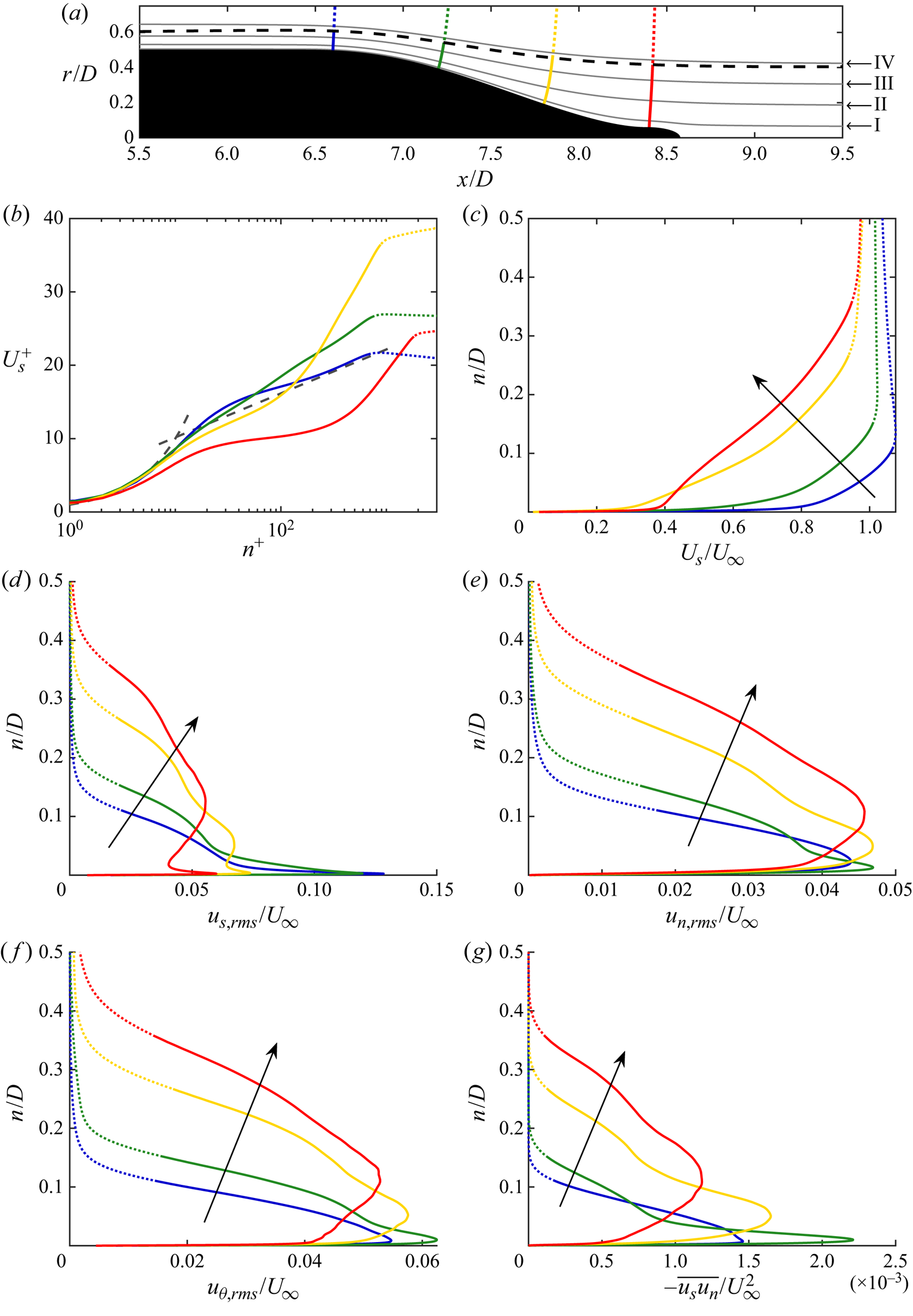
Figure 18. Evolution of the stern boundary layer plotted with streamwise-normal lines originating from the hull surface at  $x/D = 6.6$, 7.2, 7.8, 8.4 (a). Also plotted are streamlines (grey, labelled I–IV) and the boundary layer edge (black – – – –). Associated profiles of inner- and outer-scaled mean streamwise velocity (b,c), streamwise (d), streamwise-normal (e) and $\theta$-direction (f) velocity fluctuations, and Reynolds stress (g) are plotted for each potential line. Velocity profiles for the log law and viscous sublayer (grey – – – –) are also shown in panel (b). Dotted lines represent points outside of the boundary layer using the total pressure metric.
Figure 18(b,c) shows the evolution of the mean velocity along the stern. From the mid-hull to  $x/D = 6.6$, there is an initial departure from the log law as the boundary layer experiences a slight favourable pressure gradient before the body starts to taper. While the boundary layer thickness remains nearly constant, the mean velocity profile fills out and increases over the free-stream velocity before the boundary layer edge. We note that, since the favourable pressure gradient is strongest near the hull, as portrayed in figure 17(d), the vertical offset from the log law for this profile is confined to the area near the wall. This favourable pressure gradient leads to a decrease in the peak turbulence intensities between the mid-hull and this first station in the favourable pressure gradient. By the second potential line, the boundary layer experiences a strong adverse pressure gradient, and there is a higher slope of the mean velocity in the log region than the classical solution for a ZPGTBL. The turbulence intensities near the wall increase to respond to the larger streamwise pressure gradient at the wall, and a characteristic shoulder in the r.m.s. profiles forms above the peak.
By profiles three and four, the boundary layer has thickened significantly and the edge velocity is smaller than the free-stream velocity. The fourth profile shows an increase in velocity near the wall due to the locally favourable pressure gradient, but the effect of this velocity increase is confined to the flow near the wall. The profiles of  $u_{s,rms}$ for the third and fourth potential lines show a double peak, as well as a shoulder, as observed for the second profile. This double-peaked behaviour is not observed in any of the other turbulence statistics for the fourth profile. The profiles of $u_{n,rms}$, $u_{\theta ,rms}$ and $\overline {u_s u_n}$ show a broadening peak in intensities moving away from the wall and developing a second shoulder between the peak and the wall. While the peak values decrease significantly between profiles two and four for $u_{s,rms}$ and $\overline {u_s u_n}$, there is not such a strong decrease in the peaks of the $n$ and $\theta$ intensities.
Figure 19 shows contours of the  $\overline {u_s^{2}}$ and $\overline {u_s u_n}$ for the stern. Over the range $7 < x/D < 8$, there is strong generation of turbulence near the wall, which is correlated to the region of negative $D/L_a$ in figure 17(f) in the adverse pressure gradient. This is followed by a shift of the peak turbulence intensities away from the wall, with a corresponding decrease in turbulence near the wall starting at $x/D \approx 8.2$. This decrease in intensities also corresponds to the contours of positive $D/L_a$ in figure 17(f). In particular, the behaviour of the turbulence intensities seems to more closely follow the behaviour of $D/L_a$ (figure 17f) than the contour of the streamwise pressure gradient (figure 17d). We can also see a faint peak in $\overline {u_s^{2}}$ near the wall after $x/D = 8$, but no peak in the profile of $\overline {u_s u_n}$, as observed in figure 18(d,g).
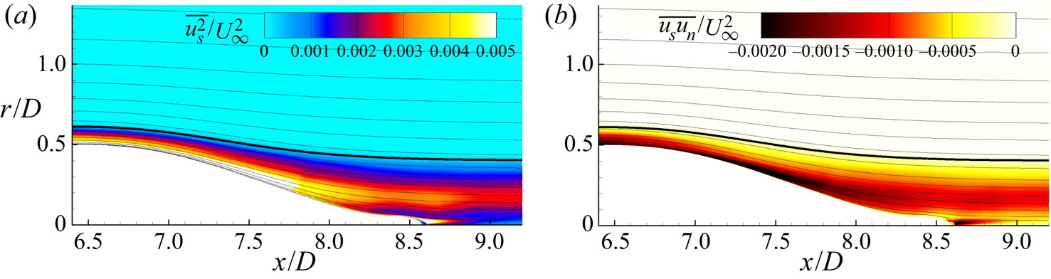
Figure 19. Contours of (a)  $\overline {u_s^{2}}$ and (b) $\overline {u_s u_n}$ non-dimensionalized by the free-stream velocity. Streamlines are shown in thin lines and the bold line represents the edge of the boundary layer.
4.9. Evolution of structures over the stern
We further investigate the evolution of the flow development along streamlines by presenting contours of instantaneous velocities in streamline coordinates for the unwrapped body of revolution defined by streamline I from figure 18(a). These surfaces are pictured in figure 20, along with dashed lines of constant  $\theta$ at intervals of ${\rm \pi} /4$ to reflect the convergence of the streamlines. Plotting contours along stream surfaces provides an opportunity to examine the development of flow structures in a frame following the mean flow. The left-hand sides of the contours of instantaneous streamline velocity and streamline velocity fluctuations in figure 20(a,b) show the characteristic streaky structures that occur in the buffer layer over the mid-hull. For $9.5 < s/D < 10$, the mean velocity increases over the favourable pressure gradient. The streaks in $u_s$ persist over this region, but there is an overall reduction in fluctuations of $u_n$. As the flow begins to decelerate under the adverse pressure gradient past $s/D = 10$, the streaky structures begin to disappear from the contour of $u_s$ and are replaced by increasingly isotropic structures. There is also a strong increase in fluctuations of $u_n$ over this region that persists into the wake. The sum of these two effects causes the instantaneous turbulent shear stress, $u_s u_n$, to increase initially over the stern despite the decrease in fluctuations of $u_s$.
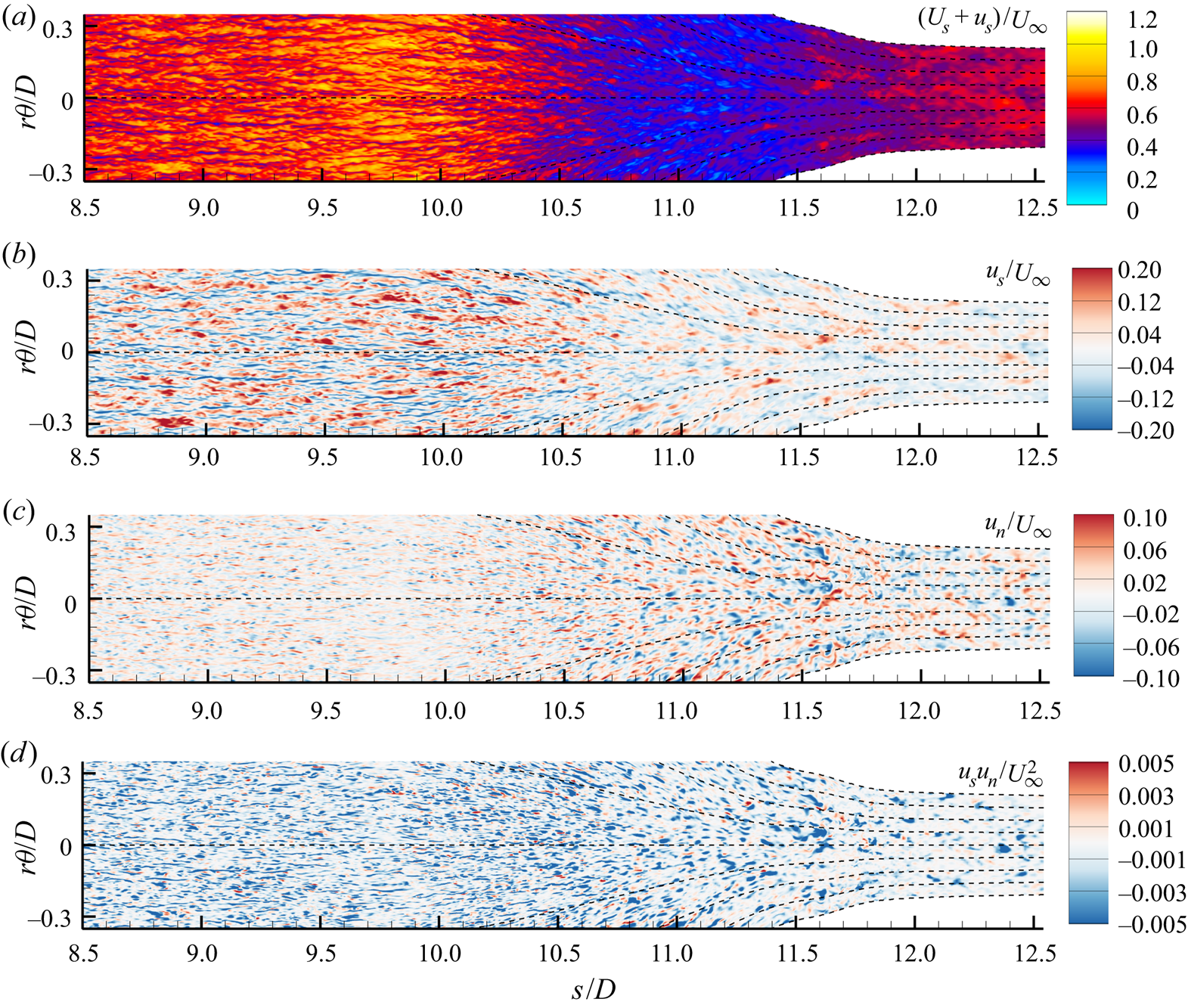
Figure 20. Unwrapped streamline surfaces of revolution for streamline I labelled in figure 18(a). Contours of instantaneous streamwise velocity (a), streamwise velocity fluctuations (b), streamline-normal velocity (c) and instantaneous turbulent shear stress (d) are plotted versus  $r\theta$ and $s$. Also plotted are lines of constant $\theta$ at intervals of ${\rm \pi} /4$ (- - - - - -) to highlight the convergence of the mean streamlines.
4.10. Stern boundary layer momentum balance
Figures 21, 22 and 23 show profiles of the streamline and streamline-normal terms from the boundary layer equations (4.6) for the second, third and fourth potential lines in figure 18. Whereas the momentum budgets for the bow were simplified by the lack of turbulence terms and the budgets for the mid-hull had no streamwise pressure gradients or streamline curvature, all of the terms in (4.6) are of leading order for flow over the stern. While the mean advection term for the boundary layer on the mid-hull approaches zero outside of the boundary layer, this is not the case for the pressure gradient boundary layer on the stern. The streamwise pressure gradient and the mean advection exactly balance outside of the boundary layer, but the no-slip condition requires zero mean advection at the wall. The adverse pressure gradient is therefore balanced by the gradient of  $\overline {u_s u_n}$ and the gradient of the viscous stress.
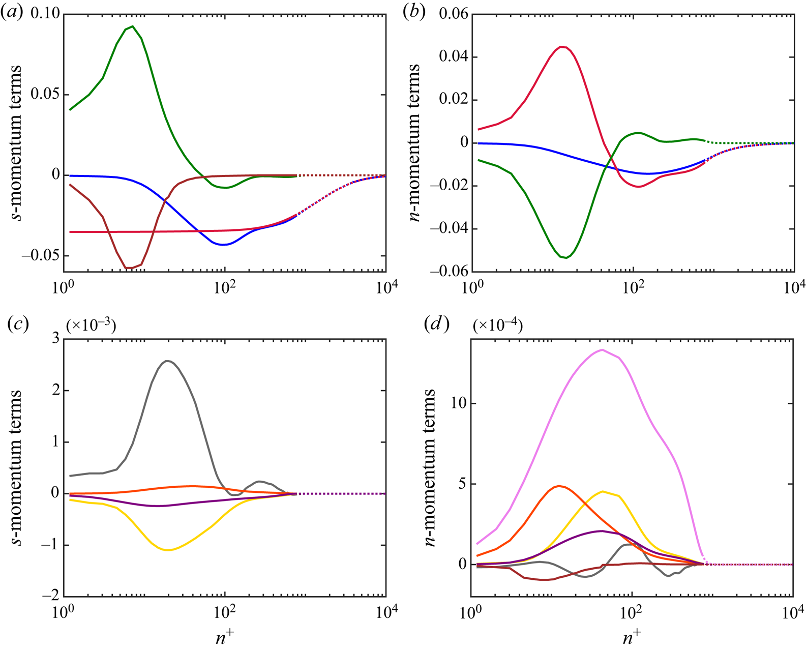
Figure 21. Profiles of terms in the mean momentum equations for the potential line emanating from  $x/D = 7.2$ on the hull surface (the second potential line from figure 18a). (a) Terms in the streamwise momentum equation: $U_s ({\partial U_s}/{\partial s})$ (blue), $-({1}/{\rho } )({\partial P}/{\partial s})$ (red), $- ({1}/{r} )({\partial }/{\partial n}) ( r \overline {u_s u_n})$ (green) and $({1}/{r})({\partial U_s}/{\partial n }) ( r \nu ({\partial U_s}/{\partial n}) )$ (brown). (b) Terms in the streamwise-normal momentum equation: ${U_s^{2}}/{R_s}$ (blue), $-({1}/{\rho } )({\partial P}/{\partial n})$ (red) and $-({1}/{r} )({\partial }/{\partial n}) ( r \overline {u_n^{2}} )$ (green). (c) Also shown are non-leading-order terms from the streamwise momentum equation: $- {\partial \overline {u_s^{2}}}/{\partial s}$ (grey), $({\overline {u_s^{2}} - \overline {u_n^{2}}})/{L_a}$ (yellow), ${2 \overline {u_s u_n}}/{R_s}$ (orange) and $(\overline {u_{\theta }^{2}} - \overline {u_n^{2}} ) ({1}/{r} )({\partial r}/{\partial s})$ (purple). (d) Non-leading-order terms in the streamline-normal direction: ${\partial \overline {u_s u_n}}/{\partial s}$ (grey), ${2 \overline {u_s u_n}}/{L_a}$ (yellow), $({\overline {u_n^{2}} - \overline {u_s^{2}}})/{R_s}$ (orange), $\overline {u_s u_n} ({1}/{r} )({\partial r}/{\partial s})$ (purple), $\overline {u_{\theta }^{2}} ({1}/{r} )({\partial r}/{\partial n})$ (pink) and the viscous term (brown). All terms are non-dimensionalized using inner scales ( $\nu /u_{\tau }^{3}$). Dotted lines represent points outside of the boundary layer.
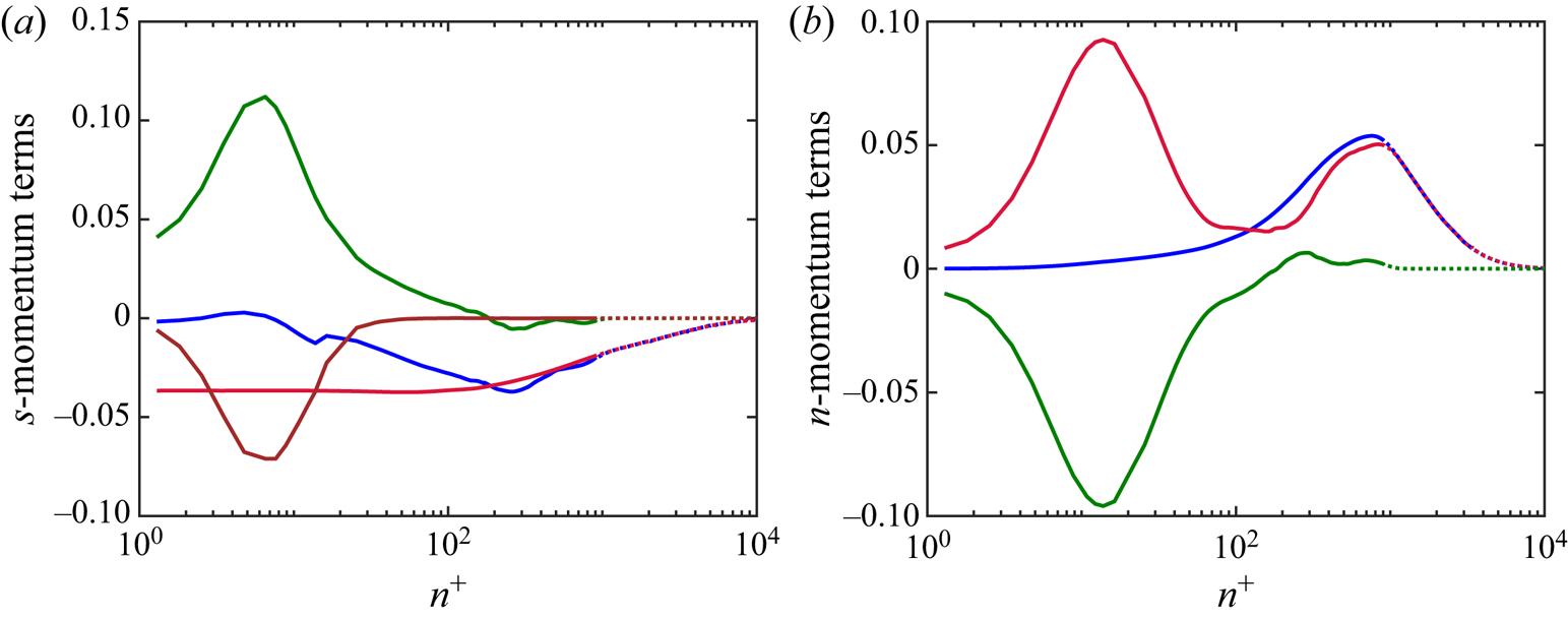
Figure 22. Profiles of terms in the boundary layer equations for the potential line emanating from  $x/D = 7.8$ on the hull surface (the third potential line from figure 18a). Terms in the streamwise momentum equation (a) follow the same colours as described in the caption for figure 21(a), as do terms in the streamwise-normal momentum equation (b) for figure 21(b). All terms are non-dimensionalized using inner scales ( $\nu /u_{\tau }^{3}$). Dotted lines represent points outside of the boundary layer using the total pressure metric.
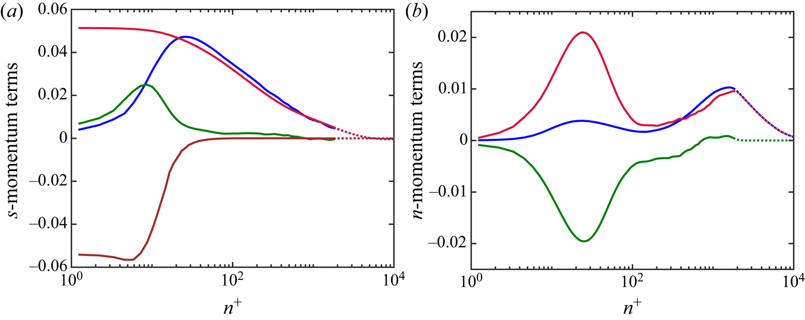
Figure 23. Profiles of terms in the boundary layer equations for the potential line emanating from  $x/D = 8.4$ on the hull surface (the last potential line from figure 18a). Terms in the streamwise momentum equation (a) follow the same colours as described in the caption for figure 21(a), as do terms in the streamwise-normal momentum equation (b) for figure 21(b). All terms are non-dimensionalized using inner scales ( $\nu /u_{\tau }^{3}$). Dotted lines represent points outside of the boundary layer.
The smaller terms in the streamline momentum balance are plotted in figure 21(c). Clearly, all of these terms are at least an order of magnitude smaller than the dominant momentum terms. The largest of these smaller terms are the streamwise gradient of  $\overline {u_s^{2}}$ and the turbulence term containing the curvature $1/L_a$. Figure 21(b) shows profiles of the streamwise-normal momentum terms. The streamline-normal pressure gradient in the boundary layer is now influenced by both the streamline curvature and the streamline-normal derivative of $\overline {u_n^{2}}$. In the outer region of the boundary layer, the pressure gradient is dominated by the effect of streamline curvature, but, as $U_s$ approaches zero near the wall, the $U_s^{2}/R_s$ term vanishes and the pressure gradient is determined by the gradient of $\overline {u_n^{2}}$. This causes the streamline-normal pressure gradient to switch signs in the log layer. The smaller terms in the streamline-normal momentum equation are plotted in figure 21(d) and are one to two orders of magnitude smaller than the dominant terms. The strongest of these terms is the turbulence term associated with $\overline {u_{\theta }^{2}}$.
Figure 22 shows profiles of the dominant momentum equation terms for the potential line projecting from  $x/D = 7.8$ on the hull surface (the third potential line from figure 18). Despite the adverse pressure gradient, there is a small streamwise acceleration near the wall due to the persisting gradient of the Reynolds stress produced in the adverse-pressure-gradient region. This is reflected in the contour of $D/L_a$ in figure 17(f). Figure 22(b) shows that the behaviour of the streamwise-normal pressure gradient has changed significantly from the profile in figure 21(b). The streamlines have changed from convex to concave curvature by this point, meaning that the curvature $1/R_s$ has changed sign. While the gradient of $\overline {u_n^{2}}$ is qualitatively similar to the profile at $x/D = 7.2$, the reversed sign of $U_s^{2}/R_s$ creates a double-peaked shape of $\partial P / \partial n$. The peak closest to the wall is due to the streamline-normal gradient of $\overline {u_n^{2}}$, while the second peak is due to the centripetal acceleration of the flow away from the wall.
This double-peak behaviour persists to the fourth potential line, originating at  $x/D = 8.4$ on the hull, whose momentum budget terms are plotted in figure 23. However, the local increase in $U_s$ near the hull surface due to the favourable pressure gradient at the stern causes a second peak in $U_s^{2}/R_s$ that further contributes to the first peak observed in the profile of $\partial P / \partial n$. By this point the gradient of $\overline {u_n^{2}}$ is significantly reduced, as the peak in the turbulence intensities has moved away from the wall. In figure 23(a), we now see a favourable streamwise pressure gradient throughout the boundary layer, forcing the viscous stress gradient to increase near the wall to satisfy the no-slip boundary condition. In the log region, the advection term is strongly dominated by the pressure gradient due to the significant decrease in the Reynolds stress gradient by this point in the boundary layer.
Analysis in streamline coordinates proves to be invaluable in understanding the mechanics of the thick boundary layer at the stern of the axisymmetric hull. In addition to the intuitive nature of the streamline-aligned equations, the explicit inclusion of the local streamline curvature in the governing equations allows for the analysis of streamline curvature variations and momentum balances in a manner that is not possible with alternative coordinate systems.
5. Conclusions
Newly derived mean momentum equations were presented for the axisymmetric streamline coordinate system and the advantages of analysis in this frame were demonstrated by LES of the DARPA SUBOFF hull geometry. While traditional cylindrical or surface-normal coordinate systems struggle to describe the flow around curved geometries such as the SUBOFF hull, the streamline coordinate system proves to be a natural frame in which to study such geometries, while also allowing direct comparison between other two-dimensional boundary layers. The streamwise momentum equation intuitively reduces to the differential form of the Bernoulli equation outside of the boundary layer. Inside of the boundary layer, this property proves useful due to the strong interaction of the outer boundary layer and the surrounding potential flow for thick axisymmetric boundary layers, as observed by Patel et al. (Reference Patel, Nakayama and Damian1974). The streamwise-normal momentum equation represents the balance of centripetal force required for fluid parcels to follow curved streamlines. This equation reduces to the Euler equation for curved streamlines outside of the boundary layer, where the streamwise-normal pressure gradient exactly balances the centripetal acceleration of the fluid ( $U_s^{2}/R_s$). Application of this equation explains the variation of static pressure inside the thick stern boundary layers as observed for streamlined axisymmetric bodies (Patel et al. Reference Patel, Nakayama and Damian1974).
LES of the SUBOFF hull geometry at  $Re_L = 1.1 \times 10^{6}$ was performed and showed good agreement with available experimental data. The results of the LES were analysed in terms of the newly derived governing equations in streamline coordinates. The front of the hull consists of a thin laminar boundary layer developing over the curved hull surface before the trip location. The governing equations in this regime can be simplified into a balance of only the mean advection, centripetal acceleration, pressure gradients and viscous force. Over the parallel mid-hull, a ZPG axisymmetric TBL develops, which leads to a simple balance of mean momentum between the gradient of the viscous stress and the gradient of the Reynolds shear stress to determine the mean advection. The tapering stern of the SUBOFF hull leads to the re-emergence of all terms in the momentum equations, with the pressure gradients in the boundary layer being strongly affected by both the turbulent stresses and the streamline curvature. Overall, the formulation of the boundary layer equations in the streamline coordinate system is promising to develop insights into the analysis of general attached two-dimensional and axisymmetric boundary layers developing over curved geometries.
Acknowledgements
The authors thank Dr S. Anantharamu for the parallel grid preprocessing for this case and Dr P. Kumar, Dr W. Horne and Mr T. Kroll for their help and discussions. Computing resources for the present work were provided by the US Army Engineer Research and Development Center (ERDC) in Vicksburg, Mississippi, on the Onyx supercomputer of the High Performance Computing Modernization Program.
Funding
This work is supported by the United States Office of Naval Research (ONR) under ONR grant N00014-18-1-2356 with Dr K.-H. Kim as technical monitor.
Declaration of Interests
The authors report no conflict of interest.
Appendix A. Transformation of the mean momentum equations into the streamline coordinate frame
In the derivation of the mean momentum equations, it is first useful to define the non-zero Christoffel symbols in terms of physical components using (2.19). These definitions are provided in table 3, and will be used in combination with (2.13)–(2.16) throughout the derivation.
Table 3. Non-zero Christoffel symbols for the metric tensor in (2.12) written in terms of physical components.
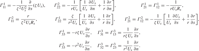
The transformation of the streamline momentum equation begins with taking the  $i=1$ component of (2.22):
 \begin{equation} \underbrace{\vphantom{\frac{g^{11}}{\rho}} \frac{\partial U^{1}}{\partial t}}_{\textrm{I}} + \underbrace{\vphantom{\frac{g^{11}}{\rho}} U^{1} U_{,1}^{1}}_{\textrm{II}} ={-} \underbrace{\frac{g^{11}}{\rho} P_{,1}}_{\textrm{III}} - \underbrace{\vphantom{\frac{g^{11}}{\rho}} \frac{\partial \overline{u^{1} u^{j}}}{\partial x^{j}}}_{\textrm{IV}} - \underbrace{\vphantom{\frac{g^{11}}{\rho}} \varGamma_{hj}^{1} \overline{u^{h} u^{j}}}_{\textrm{V}} - \underbrace{\vphantom{\frac{g^{11}}{\rho}} \varGamma_{hj}^{j} \overline{u^{1} u^{h}}}_{\textrm{VI}}+ \underbrace{\vphantom{\frac{g^{11}}{\rho}} \nu g^{jk} U_{,jk}^{1}}_{\textrm{VII}} . \end{equation}
Considering terms one-by-one, we have the following.
(i) Term I:
(A 2)\begin{equation} \frac{\partial U^{1}}{\partial t} = \frac{\partial}{\partial t} ( \zeta U_s^{2} ) = \zeta U_s \left[ \frac{\partial U_s}{\partial t} + U_s \frac{\partial \ln(\zeta U_s)}{\partial t} \right]. \end{equation}(ii) Term II:
(A 3)\begin{equation} U^{1} U_{,1}^{1} = \zeta U_s^{2} \left[ \frac{\partial U^{1}}{\partial x^{1}} + \varGamma_{11}^{1} U^{1} \right] = \zeta U_s^{2} \frac{\partial U_s}{\partial s}. \end{equation}(iii) Term III:
(A 4)\begin{equation} \frac{g^{11}}{\rho} P_{,1} = \frac{1}{\rho} \zeta^{2} U_s^{2} \frac{\partial P}{\partial x^{1}} = \zeta U_s \frac{1}{\rho} \frac{\partial P}{\partial s}. \end{equation}(iv) Term IV:
(A 5)\begin{align} \frac{\partial \overline{u^{1}u^{j}}}{\partial x^{j}} &= \frac{\partial \overline{u^{1}u^{1}}}{\partial x^{1}} + \frac{\partial \overline{u^{1}u^{2}}}{\partial x^{2}} = \frac{1}{\zeta U_s} \frac{\partial}{\partial s} ( \zeta^{2} U_s^{2} \overline{u_s^{2}} ) + \frac{1}{r U_s} \frac{\partial}{\partial n} ( r \zeta U_s^{2} \overline{u_s u_n} ) \nonumber\\ &= \zeta U_s \left[ \frac{\partial \overline{u_s^{2}}}{\partial s} + \frac{\partial \overline{u_s u_n}}{\partial n} + \frac{2\overline{u_s^{2}}}{\zeta U_s} \frac{\partial}{\partial s} (\zeta U_s) + \frac{\overline{u_s u_n}}{R_s} + \frac{\overline{u_s u_n}}{U_s} \frac{\partial U_s}{\partial n} + \frac{\overline{u_s u_n}}{r} \frac{\partial r}{\partial n} \right]. \end{align}(v) Term V:
(A 6)\begin{align} \varGamma_{hj}^{1} \overline{u^{h} u^{j}} &= \varGamma_{1j}^{1} \overline{u^{1} u^{j}} + \varGamma_{2j}^{1} \overline{u^{2} u^{j}} + \varGamma_{3j}^{1} \overline{u^{3} u^{j}} \nonumber\\ &= \varGamma_{11}^{1} \overline{u^{1} u^{1}} + \varGamma_{22}^{1} \overline{u^{2} u^{2}} + \varGamma_{33}^{1} \overline{u^{3} u^{3}} + 2\varGamma_{12}^{1} \overline{u^{1} u^{2}} \nonumber\\ &= \zeta U_s \left[- \frac{\overline{u_s^{2}}}{\zeta U_s} \frac{\partial}{\partial s} (\zeta U_s) + \frac{\overline{u_n^{2}}}{U_s} \frac{\partial U_s}{\partial s} + \frac{\overline{u_n^{2}}}{r} \frac{\partial r}{\partial s} - \frac{\overline{u_{\theta}^{2}}}{r} \frac{\partial r}{\partial s} - \frac{2 \overline{u_s u_n}}{R_s} \right]. \end{align}(vi) Term VI:
(A 7)\begin{align} \varGamma_{hj}^{j} \overline{u^{1} u^{h}} &= \varGamma_{1j}^{j} \overline{u^{1} u^{1}} + \varGamma_{2j}^{j} \overline{u^{1} u^{2}} + \varGamma_{3j}^{j} \overline{u^{1} u^{3}}\nonumber\\ &= \overline{u^{1} u^{1}} ( \varGamma_{11}^{1} + \varGamma_{12}^{2} + \varGamma_{13}^{3} ) + \overline{u^{1} u^{2}} ( \varGamma_{21}^{1} + \varGamma_{22}^{2} + \varGamma_{23}^{3} ) \nonumber\\ &= \zeta U_s \left[ -\frac{\overline{u_s^{2}}}{\zeta U_s} \frac{\partial}{\partial s} (\zeta U_s) -\frac{\overline{u_s^{2}}}{U_s} \frac{\partial U_s}{\partial s} - \frac{\overline{u_s u_n}}{R_s} - \frac{\overline{u_s u_n}}{U_s} \frac{\partial U_s}{\partial n} \right]. \end{align}(vii) Term VII:
(A 8)where
\begin{align} \nu g^{jk} U_{,jk}^{1} &=
\nu [ g^{11} U_{,11}^{1} + g^{22} U_{,22}^{1} + g^{33}
U_{,33}^{1} ] \nonumber\\ &= \nu \left[ \zeta^{2} U_s^{2}
( U_{,1}^{1} )_{,1} + r^{2} U_s^{2}
( U_{,2}^{1} )_{,2} + \frac{1}{r^{2}}
( U_{,3}^{1} )_{,3} \right],
\end{align}
(A 9)\begin{align} ( U_{,1}^{1} )_{,1} &= \frac{\partial U_{,1}^{1}}{\partial x^{1}} + \varGamma_{m1}^{1} U_{,1}^{m} - \varGamma_{11}^{m} U_{,m}^{1} \nonumber\\ &= \frac{\partial U_{,1}^{1}}{\partial x^{1}} + \varGamma_{21}^{1} U_{,1}^{2} - \varGamma_{11}^{2} U_{,2}^{1} \nonumber\\ &= \frac{\partial}{\partial x^{1}} \left( \frac{\partial U^{1}}{\partial x^{1}} + \varGamma_{11}^{1} U^{1} \right) + \varGamma_{21}^{1} ( \varGamma_{11}^{2} U^{1} ) - \varGamma_{11}^{2} \left( \frac{\partial U^{1}}{\partial x^{2}} + \varGamma_{12}^{1} U^{1} \right) \nonumber\\ &= \frac{1}{\zeta U_s} \left[ \frac{\partial^{2} U_s}{\partial s^{2}} - \frac{1}{R_s} \frac{\partial U_s}{\partial n} - \frac{U_s}{R_s^{2}} \right], \end{align}(A 10)and\begin{align} ( U_{,2}^{1} )_{,2} &= \frac{\partial U_{,2}^{1}}{\partial x^{2}} + \varGamma_{m2}^{1} U_{,2}^{m} - \varGamma_{22}^{m} U_{,m}^{1} \nonumber\\ &= \frac{\partial U_{,2}^{1}}{\partial x^{2}} + ( \varGamma_{12}^{1} - \varGamma_{22}^{2} ) U_{,2}^{1} + \varGamma_{22}^{1} ( U_{,2}^{2} - U_{,1}^{1} ) \nonumber\\ &= \frac{\partial}{\partial x^{2}}\left( \frac{\partial U^{1}}{\partial x^{2}} + \varGamma_{12}^{1} U^{1} \right) + ( \varGamma_{12}^{1} - \varGamma_{22}^{2} ) \left( \frac{\partial U^{1}}{\partial x^{2}} + \varGamma_{12}^{1} U^{1} \right) \nonumber\\ &\quad +\varGamma_{22}^{1} \left( \varGamma_{12}^{2} U^{1} - \frac{\partial U^{1}}{\partial x^{1}} - \varGamma_{11}^{1} U^{1} \right) \nonumber\\ &= \frac{\zeta}{r^{2} U_s} \left[ \frac{\partial^{2} U_s}{\partial n^{2}} - \frac{2}{U_s} \left( \frac{\partial U_s}{\partial s} \right)^{2} - \frac{3}{r} \frac{\partial U_s}{\partial s} \frac{\partial r}{\partial s} - \frac{U_s}{r^{2}} \left( \frac{\partial r}{\partial s} \right)^{2} \right] \end{align}(A 11)\begin{align} \left( U_{,3}^{1} \right)_{,3} &= \frac{\partial U_{,3}^{1}}{\partial x^{3}} + \varGamma_{m3}^{1} U_{,3}^{m} - \varGamma_{33}^{m} U_{,m}^{1} \nonumber\\ &= \varGamma_{33}^{1} ( U_{,3}^{3} - U_{,1}^{1} ) - \varGamma_{33}^{2} U_{,2}^{1} \nonumber\\ &= \varGamma_{33}^{1} \left( \varGamma_{13}^{3} U^{1} - \frac{\partial U^{1}}{\partial x^{1}} - \varGamma_{11}^{1} U^{1} \right) - \varGamma_{33}^{2} \left( \frac{\partial U^{1}}{\partial x^{2}} + \varGamma_{12}^{1} U^{1} \right) \nonumber\\ &= \zeta U_s r^{2} \left[ - \frac{U_s}{r^{2}} \left( \frac{\partial r}{\partial s} \right)^{2} + \frac{1}{r} \frac{\partial r}{\partial s} \frac{\partial U_s}{\partial s} + \frac{1}{r} \frac{\partial r}{\partial n} \frac{\partial U_s}{\partial n} \right]. \end{align}


Combining these terms and simplifying produces the streamline momentum equation given in (2.23).
In a similar fashion, transformation of the streamline-normal mean momentum equation begins with taking the  $i=2$ component of (2.22):
 \begin{equation} \underbrace{\vphantom{\frac{g^{22}}{\rho}} U^{1} U_{,1}^{2}}_{\textrm{I}} ={-} \underbrace{\frac{g^{22}}{\rho} P_{,2}}_{\textrm{II}} - \underbrace{\vphantom{\frac{g^{22}}{\rho}} \frac{\partial \overline{u^{2} u^{j}}}{\partial x^{j}}}_{\textrm{III}} - \underbrace{\vphantom{\frac{g^{22}}{\rho}} \varGamma_{hj}^{2} \overline{u^{h} u^{j}}}_{\textrm{IV}} - \underbrace{\vphantom{\frac{g^{22}}{\rho}} \varGamma_{hj}^{j} \overline{u^{2} u^{h}}}_{\textrm{V}}+ \underbrace{\vphantom{\frac{g^{22}}{\rho}} \nu g^{jk} U_{,jk}^{2}}_{\textrm{VI}} . \end{equation}
Again, considering terms individually, we have the following.
(i) Term I:
(A 13)\begin{equation} U^{1} U_{,1}^{2} = U^{1} \varGamma_{11}^{2} U^{1} = \frac{r U_s^{3}}{R_s}. \end{equation}(ii) Term II:
(A 14)\begin{equation} \frac{g^{22}}{\rho} P_{,2} = \frac{r^{2} U_s^{2}}{\rho} \frac{\partial P}{\partial x^{2}} = r U_s \frac{1}{\rho} \frac{\partial P}{\partial n}. \end{equation}(iii) Term III:
(A 15)\begin{align} \frac{\partial \overline{u^{2} u^{j}}}{\partial x^{j}} &= \frac{\partial \overline{u^{1} u^{2}}}{\partial x^{1}} + \frac{\partial \overline{u^{2} u^{2}}}{\partial x^{2}} \nonumber\\ &= \frac{1}{\zeta U_s} \frac{\partial}{\partial s} ( r \zeta U_s^{2} \overline{u_s u_n} ) + \frac{1}{r U_s} \frac{\partial}{\partial n} ( r^{2} U_s^{2} \overline{u_n^{2}} ) \nonumber\\ &= r U_s \left[ \frac{\partial \overline{u_s u_n}}{\partial s} + \frac{\partial \overline{u_n^{2}}}{\partial n} + \overline{u_s u_n} \left( \frac{1}{\zeta U_s} \frac{\partial}{\partial s} (\zeta U_s) + \frac{1}{U_s} \frac{\partial U_s}{\partial s} + \frac{1}{r} \frac{\partial r}{\partial s} \right) \right.\nonumber\\ &\left.\quad + \, 2 \overline{u_n^{2}} \left( \frac{1}{U_s} \frac{\partial U_s}{\partial n} + \frac{1}{r} \frac{\partial r}{\partial n} \right)\right]. \end{align}(iv) Term IV:
(A 16)\begin{align} \varGamma_{hj}^{2} \overline{u^{h} u^{j}} &= \varGamma_{1j}^{2} \overline{u^{1} u^{j}} + \varGamma_{2j}^{2} \overline{u^{2} u^{j}} + \varGamma_{3j}^{2} \overline{u^{3} u^{j}} \nonumber\\ &= \varGamma_{11}^{2} \overline{u^{1} u^{1}} + \varGamma_{22}^{2} \overline{u^{2} u^{2}} + \varGamma_{33}^{2} \overline{u^{3} u^{3}} + 2 \varGamma_{21}^{2} \overline{u^{1} u^{2}} \nonumber\\ &= r U_s \left[ \frac{\overline{u_s^{2}}}{R_s} - \frac{\overline{u_n^{2}}}{U_s} \frac{\partial U_s}{\partial n} - \frac{\overline{u_n^{2}}}{r} \frac{\partial r}{\partial n} - \frac{\overline{u_{\theta}^{2}}}{r} \frac{\partial r}{\partial n} - \frac{2 \overline{u_s u_n}}{U_s}\frac{\partial U_s}{\partial s} - \frac{2 \overline{u_s u_n}}{r} \frac{\partial r}{\partial s}\right]. \end{align}(v) Term V:
(A 17)\begin{align} \varGamma_{hj}^{j} \overline{u^{2} u^{h}} &= \varGamma_{1j}^{j} \overline{u^{2} u^{1}} + \varGamma_{2j}^{j} \overline{u^{2} u^{2}} + \varGamma_{3j}^{j} \overline{u^{2} u^{3}} \nonumber\\ &= \overline{u^{1} u^{2}} ( \varGamma_{11}^{1} + \varGamma_{12}^{2} + \varGamma_{13}^{3} ) + \overline{u^{2} u^{2}} ( \varGamma_{21}^{1} + \varGamma_{22}^{2} + \varGamma_{23}^{3} ) \nonumber\\ &= r U_s \left[ - \frac{\overline{u_s u_n}}{\zeta U_s} \frac{\partial}{\partial s} (\zeta U_s) - \frac{\overline{u_s u_n}}{U_s} \frac{\partial U_s}{\partial s} - \frac{\overline{u_n^{2}}}{R_s} - \frac{\overline{u_n^{2}}}{U_s} \frac{\partial U_s}{\partial n} \right]. \end{align}(vi) Term VI:
(A 18)where\begin{align} \nu g^{jk} U_{,jk}^{2} &= \nu [ g^{11} U_{,11}^{2} + g^{22} U_{,22}^{2} + g^{33} U_{,33}^{2} ] \nonumber\\ &= \nu \left[ \zeta^{2} U_s^{2} ( U_{,1}^{2} )_{,1} + r^{2} U_s^{2} ( U_{,2}^{2} )_{,2} + \frac{1}{r^{2}} ( U_{,3}^{2} )_{,3} \right], \end{align}(A 19)\begin{align} ( U_{,1}^{2} )_{,1} &= \frac{\partial U_{,1}^{2}}{\partial x^{1}} + \varGamma_{m1}^{2} U_{,1}^{m} - \varGamma_{11}^{m} U_{,m}^{2} \nonumber\\ &= \frac{\partial U_{,1}^{2}}{\partial x^{1}} + \varGamma_{11}^{2} ( U_{,1}^{1} - U_{,2}^{2} ) + ( \varGamma_{21}^{2} - \varGamma_{11}^{1} ) U_{,1}^{2} \nonumber\\ &= \frac{\partial}{\partial x^{1}} ( \varGamma_{11}^{2} U^{1} ) + \varGamma_{11}^{2} \left( \frac{\partial U^{1}}{\partial x^{1}} + \varGamma_{11}^{1} U^{1} - \varGamma_{12}^{2} U^{1} \right) + ( \varGamma_{21}^{2} - \varGamma_{11}^{1} ) ( \varGamma_{11}^{2} U^{1} )\nonumber\\ &= \frac{r}{\zeta^{2} U_s} \left[ \frac{2}{R_s} \frac{\partial U_s}{\partial s} + \frac{\partial}{\partial s} \left( \frac{U_s}{R_s} \right) + \frac{U_s}{rR_s} \frac{\partial r}{\partial s} \right], \end{align}(A 20)and\begin{align} ( U_{,2}^{2} )_{,2} &= \frac{\partial U_{,2}^{2}}{\partial x^{2}} + \varGamma_{m2}^{2} U_{,2}^{m} - \varGamma_{22}^{m} U_{,m}^{2} \nonumber\\ &= \frac{\partial U_{,2}^{2}}{\partial x^{2}} + \varGamma_{12}^{2} U_{,2}^{1} - \varGamma_{22}^{1} U_{,1}^{2} \nonumber\\ &= \frac{\partial}{\partial x^{2}} ( \varGamma_{12}^{2} U^{1} ) + \varGamma_{12}^{2} \left( \frac{\partial U^{1}}{\partial x^{2}} + \varGamma_{12}^{1} U^{1} \right) - \varGamma_{22}^{1} ( \varGamma_{11}^{2} U^{1} ) \nonumber\\ &=\frac{1}{r U_s} \left[- \frac{1}{R_s} \frac{\partial U_s}{\partial s} - \frac{U_s}{r R_s} \frac{\partial r}{\partial s} - \frac{1}{U_s} \frac{\partial U_s}{\partial s} \frac{\partial U_s}{\partial n} - \frac{2}{r} \frac{\partial r}{\partial s} \frac{\partial U_s}{\partial n} \right.\nonumber\\ & \left.\quad -\,\frac{\partial^{2} U_s}{\partial n \partial s} - \frac{U_s}{r} \frac{\partial^{2} r}{\partial n \partial s} + \frac{U_s}{r^{2}} \frac{\partial r}{\partial s} \frac{\partial r}{\partial n} \right] \end{align}(A 21)\begin{align} ( U_{,3}^{2} )_{,3} &= \frac{\partial U_{,3}^{2}}{\partial x^{3}} + \varGamma_{m3}^{2} U_{,3}^{m} - \varGamma_{33}^{m} U_{,m}^{2} \nonumber\\ &= \varGamma_{33}^{2} ( U_{,3}^{3} - U_{,2}^{2} ) - \varGamma_{33}^{1} U_{,1}^{2} \nonumber\\ &= \varGamma_{33}^{2} ( \varGamma_{13}^{3} U^{1} - \varGamma_{12}^{2} U^{1} ) - \varGamma_{33}^{1} ( \varGamma_{11}^{2} U^{1} ) \nonumber\\ &= r^{2} U_s \left[ \frac{U_s}{r R_s} \frac{\partial r}{\partial s} - \frac{1}{r} \frac{\partial r}{\partial n} \frac{\partial U_s}{\partial s} - \frac{2 U_s}{r^{2}} \frac{\partial r}{\partial n} \frac{\partial r}{\partial s} \right]. \end{align}


Combining these terms and simplifying produces the streamline-normal momentum equation given in (2.28).


 Open access