


1. Introduction
Electrosprays operating in the cone-jet mode (Zeleny Reference Zeleny1917; Taylor Reference Taylor1964; Cloupeau & Prunet-Foch Reference Cloupeau and Prunet-Foch1989; Fernández De La Mora & Loscertales Reference Fernández De La Mora and Loscertales1994; Collins et al. Reference Collins, Jones, Harris and Basaran2008) have the unique ability for producing sprays of charged droplets with narrow size distributions, down to radii of a few nanometres (De Juan & Fernández De La Mora Reference De Juan and Fernández De La Mora1997; Rosell-Llompart, Grifoll & Loscertales Reference Rosell-Llompart, Grifoll and Loscertales2018). The fate of these droplets is governed by the amount of charge they carry relative to their size which, when sufficiently high, can lead to the disintegration of the droplet and/or the shedding of charge by ion field emission. Rayleigh (Reference Rayleigh1882) predicted that a spherical droplet charged beyond a critical value, referred to as the Rayleigh limit, is unstable and will disintegrate. This process is called the Rayleigh fission or Coulomb explosion of the droplet. The pressures inside and outside of the droplet are equal at the Rayleigh limit, i.e. the mechanical and electrical contributions to the surface tension cancel out one another (Rayleigh Reference Rayleigh1882; Taylor Reference Taylor1964; Basaran & Scriven Reference Basaran and Scriven1989). This condition can be written in terms of the charge  $Q_{Ray}$ carried by the droplet or the strength of the electric field $E_{Ray}$ on its surface:
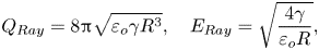 \begin{equation} Q_{Ray}=8{\rm \pi}\sqrt{\varepsilon_{o} \gamma R^{3}}, \quad E_{Ray}=\sqrt{\frac{4\gamma}{\varepsilon_{o}R}}, \end{equation}
where  $\gamma$ and $R$ are the surface tension and the radius of the droplet, respectively, and $\varepsilon _{o}$ is the permittivity of vacuum. A droplet charged at or above the Rayleigh limit will undergo a Coulomb explosion, shedding a fraction of its charge and mass in the form of smaller progeny droplets. Interested readers may refer to the photographs of Coulomb explosions taken by Gomez & Tang (Reference Gomez and Tang1994), Duft et al. (Reference Duft, Achtzehn, Müller, Huber and Leisner2003) and Giglio et al. (Reference Giglio, Gervais, Rangama, Manil, Huber, Duft, Müller, Leisner and Guet2008).
The prediction of Rayleigh motivated several experimental studies. Doyle, Moffett & Vonnegut (Reference Doyle, Moffett and Vonnegut1964) used Millikan's oil drop technique to study the Coulomb explosion of evaporating aniline and water droplets. They estimated a charge loss of roughly  $30\,\%$ in the form of smaller progeny droplets, with very low mass loss. Schweizer & Hanson (Reference Schweizer and Hanson1971) reported a charge and mass loss of $25\,\%$ and $5\,\%$, respectively. Duft et al. (Reference Duft, Achtzehn, Müller, Huber and Leisner2003) used an electrohydrodynamic levitation technique coupled with high-resolution time-elapse photography to isolate a charged droplet and capture the transient behaviour of the Coulomb explosion; they reported a charge loss of $33\,\%$ and a mass loss smaller than $1\,\%$. Giglio et al. (Reference Giglio, Gervais, Rangama, Manil, Huber, Duft, Müller, Leisner and Guet2008) conducted similar experiments and also performed numerical simulations. They also reported an experimental charge loss of $33\,\%$. Other studies report charge losses between $20\,\%\unicode{x2013}40\,\%$ (Roulleau & Desbois Reference Roulleau and Desbois1972; Taflin, Ward & Davis Reference Taflin, Ward and Davis1989), with the exception of sulphuric acid droplets which lose
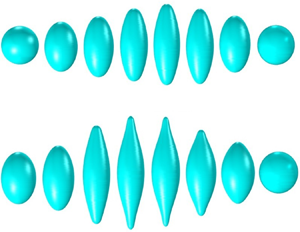
  $50\,\%$ of their original charge (Richardson, Pigg & Hightower Reference Richardson, Pigg and Hightower1989). The images captured by Duft et al. (Reference Duft, Achtzehn, Müller, Huber and Leisner2003) and Giglio et al. (Reference Giglio, Gervais, Rangama, Manil, Huber, Duft, Müller, Leisner and Guet2008) have encouraged analytical and numerical computations of the transient behaviour of exploding droplets under different Reynolds numbers (Betelú et al. Reference Betelú, Fontelos, Kindelán and Vantzos2006; Burton & Taborek Reference Burton and Taborek2011; Collins et al. Reference Collins, Sambath, Harris and Basaran2013; Radcliffe Reference Radcliffe2013; Garzon, Gray & Sethian Reference Garzon, Gray and Sethian2014; Gawande, Mayya & Thaokar Reference Gawande, Mayya and Thaokar2017, Reference Gawande, Mayya and Thaokar2020). The experimental and numerical evidence show that a Coulomb explosion can be described as a three-step process: first, the slightly perturbed spherical droplet elongates into an ellipsoid of increasing aspect ratio, which eventually develops conical tips at the vertices; second, a fine jet is issued from each cusp and accelerated by the axial electric field; third, the jets, which are naturally unstable, break into progeny droplets which may undergo further Coulomb explosions depending on their electrification level.
Ion field emission is a second mechanism by which a droplet can shed charge. It is a kinetic process in which ions evaporating from the surface of a liquid must overcome an energy barrier (the ion solvation energy), which is lowered by the electric field. Early experiments demonstrated that ion field emission occurs in charged nanodroplets (Iribarne & Thomson Reference Iribarne and Thomson1976; Thomson & Iribarne Reference Thomson and Iribarne1979; Katta, Rockwood & Vestal Reference Katta, Rockwood and Vestal1991). Loscertales & Fernández De La Mora (Reference Loscertales and Fernández De La Mora1995) analysed the solid residues left behind by charged nanodroplets after complete evaporation of the liquid phase to quantify the electric field required for ion field emission. Labowsky, Fenn & Fernández De La Mora (Reference Labowsky, Fenn and Fernández De La Mora2000) developed a continuum ion evaporation model that was in good agreement with the experimental findings of Gamero-Castaño & Fernández De La Mora (Reference Gamero-Castaño and Fernández De La Mora2000b) and Hogan & Fernández De La Mora (Reference Hogan and Fernández De La Mora2009). These studies predict the electric field  $E^{*}$ necessary for ion emission to be in the range $0.8\unicode{x2013}2\,{\rm V}\,{\rm nm}^{-1}$, which is only possible in highly charged droplets with diameters of tens of nanometres or smaller. These droplets can originate from much larger droplets in aerosols, where large residence times combined with solvent evaporation lead to a chain of Coulomb explosions producing increasingly smaller droplets. Alternatively, highly charged nanodroplets can be directly produced by electrospraying liquids with high electrical conductivities (Gamero-Castaño & Cisquella-Serra Reference Gamero-Castaño and Cisquella-Serra2020; Miller et al. Reference Miller, Ulibarri-Sanchez, Prince and Bemish2021; Perez-Lorenzo & Fernández De La Mora Reference Perez-Lorenzo and Fernández De La Mora2022).
The nanodroplets produced by electrospraying highly conducting liquids are often charged above the Rayleigh limit (Gamero-Castaño & Cisquella-Serra Reference Gamero-Castaño and Cisquella-Serra2020; Miller et al. Reference Miller, Ulibarri-Sanchez, Prince and Bemish2021; Perez-Lorenzo & Fernández De La Mora Reference Perez-Lorenzo and Fernández De La Mora2022). Moreover, Gamero-Castaño & Cisquella-Serra (Reference Gamero-Castaño and Cisquella-Serra2020) and Perez-Lorenzo & Fernández De La Mora (Reference Perez-Lorenzo and Fernández De La Mora2022) observe that a significant fraction of the total current in these electrosprays is carried by ions, e.g. 20–25 % of the total current in electrosprays of EMI-Im and 1-ethyl-3-methylimidazolium tris(perfluoroethyl)trifluorophosphate (EMI-FAP). Both studies find that the ions must be evaporating from droplets in flight and propose that, in some cases, the emission occurs from droplets undergoing Coulomb explosions. The general consensus is that ions will evaporate from the surface of the droplet if the field emission limit is reached before the Rayleigh limit, i.e. if  $E_{Ray} > E^{*}$ (Iribarne & Thomson Reference Iribarne and Thomson1976; Labowsky Reference Labowsky1998; Labowsky et al. Reference Labowsky, Fenn and Fernández De La Mora2000). However, a droplet charged above the Rayleigh limit and having an electric field smaller than $E^{*}$ may develop areas with larger electric fields during the Coulomb explosion and emit ions. This shedding of charge may reduce substantially the net charge of the parent droplet, modify the dynamics of the Coulomb explosion and even prevent it.
The goal of this article is to study the interaction between a Coulomb explosion and ion field emission in highly charged nanodroplets. We develop an electrohydrodynamic, phase field model to compute the deformation of a droplet charged above the Rayleigh limit, while including ion field emission. We use this model to study EMI-Im nanodroplets in the diameter range 10–100 nm, because experiments show the simultaneous presence of Coulomb explosions and ion field emission under these conditions (Gamero-Castaño & Cisquella-Serra Reference Gamero-Castaño and Cisquella-Serra2020). We address two specific questions: the extent to which ion emission suppresses Coulomb explosions and the magnitude of the charge emitted from typical nanodroplets. The remainder of this article is organized as follows: § 2 describes the numerical model; § 3.1 analyses the Coulomb explosion in the absence of ion emission, with the goals of setting a baseline and validating the numerical model; § 3.2 analyses the effects of ion emission in droplets of varying size charged above the Rayleigh limit; and § 4 summarizes the findings and recommends future work.
2. Problem formulation and numerical set-up
2.1. Problem formulation
Figure 1 shows the computational domain in cylindrical coordinates  $\{r,z\}$. There are two subdomains, $\varOmega _{l}$ and $\varOmega _{g}$, occupied by an ionic liquid and ambient gas, respectively. The ionic liquid forms a spherical droplet of radius $R$ centred in the origin of coordinates, with a net charge exceeding the Rayleigh limit, $Q_o = \eta Q_{Ray}$ with $\eta > 1$. The droplet is slightly deformed to make it spheroidal while keeping its volume, such that the major axis (along $z$) is $1.04$ times the minor axis (Burton & Taborek Reference Burton and Taborek2011; Giglio et al. Reference Giglio, Rangama, Guillous and Le Cornu2020). The droplet is then allowed to evolve from this starting configuration. The problem exhibits axial and planar ( $z=0$) symmetries, and therefore the governing equations are solved in the quadrant bounded by segments $\varGamma _{b}$, $\varGamma _{r}$, $\varGamma _{u}$ and $\varGamma _{l}$. The viscosity, density, relative permittivity and electrical conductivity of the media are $\mu _i$, $\rho _i$, $\varepsilon _i$ and $K_i$, respectively, where the subscript $i$ denotes the ambient gas ( $g$) or the ionic liquid ( $l$).
$l$).
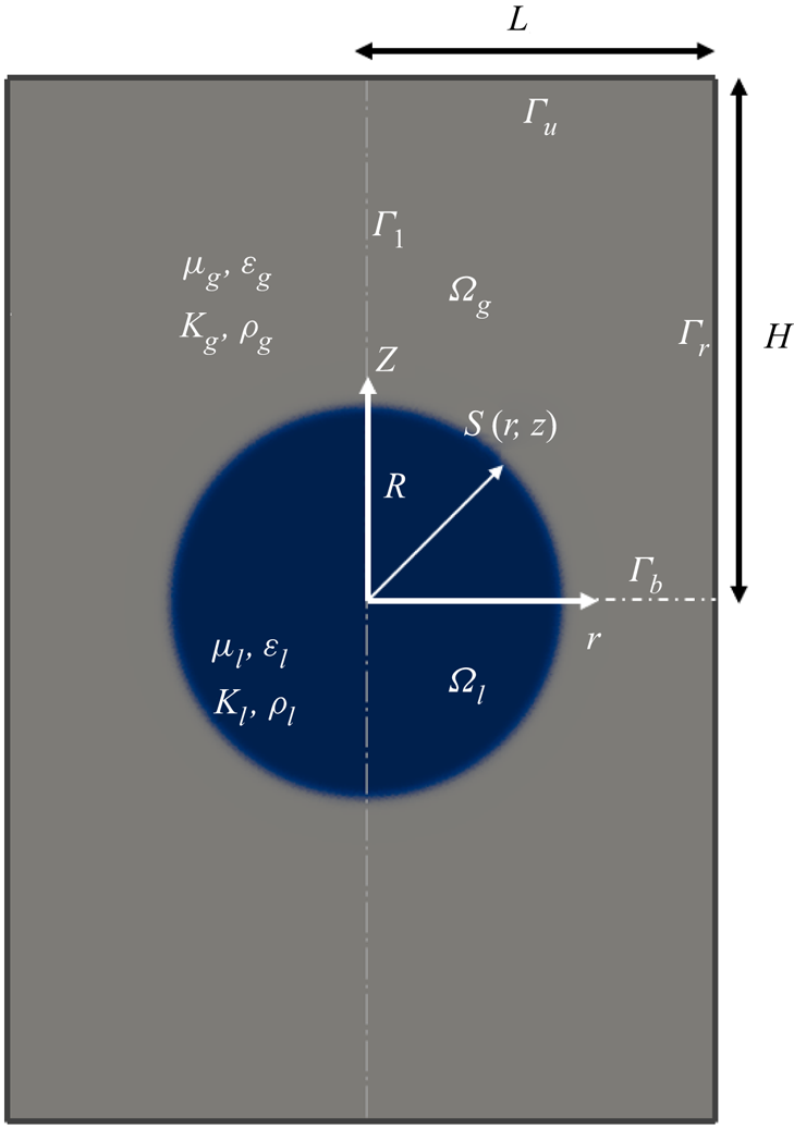
Figure 1. Schematic of the problem and computational domain.
Electrohydrodynamic problems involving a free surface are usually solved using the leaky dielectric model (Melcher & Taylor Reference Melcher and Taylor1969; Saville Reference Saville1997), which treats the interface between the liquid and the surrounding gas as a surface. All excess charge is assumed to reside on the surface (surface charge). Conservation of charge is fulfilled by imposing a conservation equation on the surface, together with an Ohms law and the assumption of negligible volumetric charge in the bulk of the liquid. Drawbacks include the difficult calculation of the position of the free surface and the failure of model assumptions in ultra-fast liquid disintegration (Ganán-Calvo et al. Reference Ganán-Calvo, López-Herrera, Rebollo-Munoz and Montanero2016; Pillai et al. Reference Pillai, Berry, Harvie and Davidson2016). To avoid these problems, we use the phase field method (Anderson, Mcfadden & Wheeler Reference Anderson, Mcfadden and Wheeler1998; Jacqmin Reference Jacqmin1999; Yue et al. Reference Yue, Feng, Liu and Shen2004). This method regards the interface as a thin region of finite thickness, which can be easily tracked, and a continuous distribution of all independent variables throughout the media. It has the additional advantage of eliminating the assumption of negligible volumetric charge in the bulk of the liquid. The phase field method has been proven to be accurate in a variety of electrohydrodynamic problems (Tomar et al. Reference Tomar, Gerlach, Biswas, Alleborn, Sharma, Durst, Welch and Delgado2007; López-Herrera, Popinet & Herrada Reference López-Herrera, Popinet and Herrada2011; López-Herrera et al. Reference López-Herrera, Gañán-Calvo, Popinet and Herrada2015; Mandal et al. Reference Mandal, Ghosh, Bandopadhyay and Chakraborty2015; Ganán-Calvo et al. Reference Ganán-Calvo, López-Herrera, Rebollo-Munoz and Montanero2016; Pillai et al. Reference Pillai, Berry, Harvie and Davidson2016).
We have previously developed an electrohydrodynamic phase field model for electrified jets and validated it with existing experimental and numerical results (Misra & Gamero-Castaño Reference Misra and Gamero-Castaño2022). The ionic liquid and the surrounding gas are modelled as a continuum by defining a scalar phase variable  $\phi$ that varies uniformly across the two media. Here, $\phi$ is tracked using the Cahn–Hilliard equations (Anderson et al. Reference Anderson, Mcfadden and Wheeler1998), which is assigned values of $-1$ and $1$ in the gas and the liquid far from the interface, respectively. The surface separating the gas and liquid phases is defined as the loci where $\phi =0$. The physical properties are defined as continuous functions of $\phi$ throughout the media. Specifically, $\rho$, $\mu$ and $\varepsilon$ are the weighted arithmetic means of the phase variable:
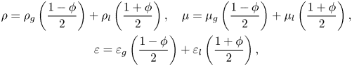 $$\begin{gather} \rho=\rho_{g}\left(\frac{1-\phi}{2}\right)+\rho_{l}\left(\frac{1+\phi}{2}\right), \quad \mu=\mu_{g}\left(\frac{1-\phi}{2}\right)+\mu_{l}\left(\frac{1+\phi}{2}\right), \nonumber\\ \varepsilon=\varepsilon_{g}\left(\frac{1-\phi}{2}\right)+\varepsilon_{l}\left(\frac{1+\phi}{2}\right), \end{gather}$$
whereas, to mitigate unphysical charge leakage, the electrical conductivity is defined as
 \begin{equation} \frac{1}{K}=\frac{1}{K_{g}}\left(\frac{1-\phi}{2}\right)+ \frac{1}{K_{l}}\left(\frac{1+\phi}{2}\right) \end{equation}
(Tomar et al. Reference Tomar, Gerlach, Biswas, Alleborn, Sharma, Durst, Welch and Delgado2007; López-Herrera et al. Reference López-Herrera, Popinet and Herrada2011; Roghair et al. Reference Roghair, Musterd, Ende, Kleijin, Kruetzer and Mugele2015; Huh & Wirz Reference Huh and Wirz2022). Presently, the model of Misra & Gamero-Castaño (Reference Misra and Gamero-Castaño2022) is supplemented with the standard transport equation for ion field emission (Iribarne & Thomson Reference Iribarne and Thomson1976; Loscertales & Fernández De La Mora Reference Loscertales and Fernández De La Mora1995):
 \begin{equation} J_{i}=\frac{k_{B}T}{h}\sigma \exp\left(-\frac{\Delta G - G(E_{n}^{g})}{k_{B}T}\right), \end{equation}
where  $J_{i}$ is the ion current density evaporated from the surface, $k_B$ is the Boltzmann constant, $T$ is the temperature of the liquid, $\sigma$ is the surface charge density and $h$ is Planck's constant. Here, $\Delta G -G(E_{n}^{g})$ is the energy barrier that the evaporating ion must overcome. Additionally, $\Delta G$ is the ion solvation energy, which is not accurately known for ionic liquids although it is estimated to be in the range of 1.4–2 eV (Iribarne & Thomson Reference Iribarne and Thomson1976; Loscertales & Fernández De La Mora Reference Loscertales and Fernández De La Mora1995; Gamero-Castaño & Fernández De La Mora Reference Gamero-Castaño and Fernández De La Mora2000a,Reference Gamero-Castaño and Fernández De La Morac). Also, $G(E_{n}^{g})$ is the reduction of the energy barrier due to the normal component of the electric field on the gas side of the surface $E_{n}^{g}$. We use the model by Iribarne & Thomson (Reference Iribarne and Thomson1976) to evaluate the reduction of the energy barrier:
 \begin{equation} G(E_{n}^{g})=\left(\frac{e^{3}E_{n}^{g}}{4{\rm \pi}\varepsilon_{o}}\right)^{1/2}, \end{equation}
where  $e$ stands for the elementary unit charge. Equation (2.3) suggests that a meaningful ion current can only occur when $\Delta G - G(E_{n}^{g})= {O}(k_{B}T)$. Since $k_{B}T \ll \Delta G$ at room conditions, the characteristic electric field for ion field emission is given by (Coffman et al. Reference Coffman, Martínez-Sánchez, Higuera and Lozano2016; Coffman, Martínez-Sánchez & Lozano Reference Coffman, Martínez-Sánchez and Lozano2019; Gallud & Lozano Reference Gallud and Lozano2022):
 \begin{equation} E^{*}=\frac{4{\rm \pi}\varepsilon_{o}{\Delta G}^{2}}{e^3}. \end{equation}
 The dependent variables velocity  $\boldsymbol {u}$, pressure $p$, volumetric charge density $\rho _e$, electric potential $V$ and the phase variable $\phi$ fulfil the equations of conservation of mass, momentum and charge, a modified Poisson's equation and the Cahn–Hillard equation throughout the computational domain:
 \begin{gather} \boldsymbol{\nabla} \boldsymbol{\cdot} \boldsymbol{u}= 0, \end{gather}
 \begin{gather} \frac{\partial(\rho \boldsymbol{u})}{\partial t}+\boldsymbol{\nabla} \boldsymbol{\cdot} (\rho \boldsymbol{u}\boldsymbol{u})={-}\boldsymbol{\nabla}p +\boldsymbol{\nabla} \boldsymbol{\cdot} (\mu (\boldsymbol{\nabla u}+\boldsymbol{\nabla u}^{\rm T}))+ \boldsymbol{F}_{es} + \boldsymbol{F}_{st}, \end{gather}
 \begin{gather} \frac{\partial\rho_e}{\partial t} +\boldsymbol{\nabla} \boldsymbol{\cdot} (\rho_e \boldsymbol{u})={-}\boldsymbol{\nabla} \boldsymbol{\cdot} (K\boldsymbol{E})-\frac{k_{B}T}{h}\rho_{e}\exp\left(-\frac{\Delta G - G(E_{n}^{g})}{k_{B}T}\right), \end{gather}
 \begin{gather} \varepsilon \nabla^{2}V + \boldsymbol{\nabla}V \boldsymbol{\cdot} \boldsymbol{\nabla}\varepsilon={-}\frac{\rho_e}{\varepsilon_{o}}, \end{gather}
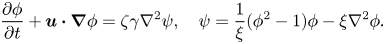 \begin{gather} \frac{\partial \phi}{\partial t} + \boldsymbol{u} \boldsymbol{\cdot} \boldsymbol{\nabla} \phi=\zeta \gamma \nabla^{2} \psi , \quad \psi=\frac{1}{\xi}(\phi^{2}-1)\phi-\xi\nabla^{2}\phi . \end{gather}
Here,  $\boldsymbol {F}_{es}$ and $\boldsymbol {F}_{st}$ are the electrostatic and surface tension volumetric forces:
 \begin{gather} \boldsymbol{F}_{es}= \boldsymbol{\nabla} \boldsymbol{\cdot} \boldsymbol{T}_{e} = \boldsymbol{\nabla} \boldsymbol{\cdot} \varepsilon \varepsilon_o\left(\boldsymbol{EE}-\frac{1}{2}\boldsymbol{I}|E|^{2}\right) = \rho_e\boldsymbol{E}-\frac{1}{2}\varepsilon_o \boldsymbol{E} \boldsymbol{\cdot} \boldsymbol{E} \boldsymbol{\nabla}\varepsilon, \end{gather}
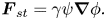 \begin{gather} \boldsymbol{F}_{st}=\gamma\psi\boldsymbol{\nabla}\phi. \end{gather}
The volumetric charge conservation equation (2.8) can be derived from the general Poisson–Nernst–Planck (PNP) equation for charged species (Saville Reference Saville1997; Herrada et al. Reference Herrada, López-Herrera, Gañán-Calvo, Vega, Montanero and Popinet2012; Gañán-Calvo et al. Reference Gañán-Calvo, López-Herrera, Herrada, Ramos and Montanero2018), see Appendix B for further details. The equation includes charge convection and conduction, and a term accounting for the loss of charge due to ion field emission. Equation (2.10a,b) is the Cahn–Hillard equation for the phase variable  $\phi$ (Anderson et al. Reference Anderson, Mcfadden and Wheeler1998; Jacqmin Reference Jacqmin1999, Reference Jacqmin2000; Yue et al. Reference Yue, Feng, Liu and Shen2004); $\zeta$ is the phase field mobility parameter (a constant) and $\xi$ is the diffuse interface thickness which is indicative of the sharpness of the artificial interface separating the two phases. Brackbill, Kothe & Zemach (Reference Brackbill, Kothe and Zemach1992), Jacqmin (Reference Jacqmin2000), Anderson et al. (Reference Anderson, Mcfadden and Wheeler1998), Jacqmin (Reference Jacqmin1999) and Yue et al. (Reference Yue, Feng, Liu and Shen2004) provide derivations of the surface tension force, (2.12). It is worth noting that in the sharp interface limit, $\xi \rightarrow 0$, the phase field formulation transforms into the conventional treatment based on the use of a surface (Brackbill et al. Reference Brackbill, Kothe and Zemach1992; Yue et al. Reference Yue, Feng, Liu and Shen2004). We employ the following boundary conditions:
 \begin{gather} \boldsymbol{e}_{z} \boldsymbol{\cdot} \boldsymbol{E} = 0, \quad \boldsymbol{e}_{z} \boldsymbol{\cdot} \boldsymbol{u} = 0, \quad \boldsymbol{e}_{z} \boldsymbol{\cdot} \boldsymbol{\nabla}\psi=\boldsymbol{e}_{z} \boldsymbol{\cdot} \boldsymbol{\nabla}\phi = 0, \quad \text{on}\ \varGamma_{b}, \end{gather}
 \begin{gather} V=0, \quad \boldsymbol{u} = 0, \quad \boldsymbol{e}_{r} \boldsymbol{\cdot} \boldsymbol{\nabla}\psi= \boldsymbol{e}_{r} \boldsymbol{\cdot} \boldsymbol{\nabla}\phi = 0, \quad \rho_{e}=0, \quad p=0, \quad \text{on}\ \varGamma_{r}, \end{gather}
 \begin{gather} V=0, \quad \boldsymbol{u} = 0, \quad \boldsymbol{e}_{z} \boldsymbol{\cdot} \boldsymbol{\nabla}\psi= \boldsymbol{e}_{z} \boldsymbol{\cdot} \boldsymbol{\nabla}\phi = 0, \quad \rho_{e}=0, \quad p=0, \quad \text{on} \varGamma_{u}, \end{gather}
 \begin{gather} \boldsymbol{e}_{r}\boldsymbol{\cdot} \boldsymbol{E}=0, \quad \frac{\partial (\boldsymbol{e}_{z}\boldsymbol{\cdot}\boldsymbol{u})}{\partial r}=\boldsymbol{e}_{r} \boldsymbol{\cdot} \boldsymbol{u}= 0, \quad \boldsymbol{e}_{r} \boldsymbol{\cdot} \boldsymbol{\nabla}\psi= \boldsymbol{e}_{r} \boldsymbol{\cdot} \boldsymbol{\nabla}\phi = 0 ,\quad \text{on}\ \varGamma_{l}. \end{gather}
 We write the system of equations in dimensionless form using  $l_c = R$, $t_c= \mu _{l}l_c/\gamma$, $u_c = l_c / t_c$, $p_c = \gamma / l_{c}$, $E_c = Q_{o}/(4 {\rm \pi}\varepsilon _{o} l_{c}^{2})$ and $\rho _{e,c}=\varepsilon _{o} E_c / l_{c}$ as the characteristic scales for length, time, velocity, pressure, electric field and volumetric charge, respectively. In particular, the dimensionless forms of the governing equations (2.6)–(2.10a,b) read
 \begin{gather} \boldsymbol{\widetilde{\nabla}} \boldsymbol{\cdot} \boldsymbol{\tilde{u}}= 0, \end{gather}
 \begin{gather} \frac{1}{{{Oh}^2}}\frac{\partial(\frac{\rho}{\rho_l} \boldsymbol{\tilde{u}})}{\partial \tilde{t}}+ \frac{1}{{{Oh}^2}}\boldsymbol{\widetilde{\nabla}} \boldsymbol{\cdot} \left(\frac{\rho}{\rho_l} \boldsymbol{\tilde{u}}\boldsymbol{\tilde{u}}\right)={-}\boldsymbol{\widetilde{\nabla}}\tilde{p} +\boldsymbol{\widetilde{\nabla}} \boldsymbol{\cdot} \left(\frac{\mu}{\mu_l} \left(\boldsymbol{\widetilde{\nabla} \tilde{u}}+\boldsymbol{\widetilde{\nabla} \tilde{u}}^{\rm T}\right)\right)+ \varGamma \boldsymbol{\tilde{F}}_{es} + \boldsymbol{\tilde{F}}_{st}, \end{gather}
 \begin{gather} {\frac{\varPi_{1}}{\varepsilon_l}} \frac{\partial\tilde{\rho}_e}{\partial \tilde{t}} + {\frac{\varPi_{1}}{\varepsilon_l}} \boldsymbol{\widetilde{\nabla}} \boldsymbol{\cdot} \left(\tilde{\rho}_e \boldsymbol{\tilde{u}}\right)={-}\boldsymbol{\widetilde{\nabla}} \boldsymbol{\cdot} \left(\frac{K}{K_l}\boldsymbol{\tilde{E}}\right)-{\frac{\varPi_{2}}{\varepsilon_l}}\tilde{\rho}_{e} \exp\left(-\varPi_{3}\left(1- \sqrt{\tilde{E}_{n}^{g}/ \varPi_{4}} \right)\right), \end{gather}
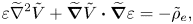 \begin{gather} \varepsilon \widetilde{\nabla}^{2}\tilde{V} + \boldsymbol{\widetilde{\nabla}}\tilde{V} \boldsymbol{\cdot} \boldsymbol{\widetilde{\nabla}}\varepsilon={-}\tilde{\rho}_e, \end{gather}
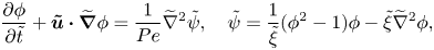 \begin{gather} \frac{\partial \phi}{\partial \tilde{t}} + \boldsymbol{\tilde{u}} \boldsymbol{\cdot} \boldsymbol{\widetilde{\nabla}} \phi= \frac{1}{{Pe}}\widetilde{\nabla}^{2} \tilde{\psi} , \quad \tilde{\psi}=\frac{1}{\tilde{\xi}}(\phi^{2}-1)\phi-\tilde{\xi}\widetilde{\nabla}^{2}\phi, \end{gather}
where dimensionless variables are designated with an overtilde. Equations (2.17)–(2.21a,b) include eight dimensionless numbers:  ${Oh}$, $\varGamma$, $\varPi _1$, $\varPi _2$, $\varPi _3$, $\varPi _4$, $Pe$ and $\varepsilon _l$. In addition, the ratios $\rho _g / \rho _l$, $\mu _g/\mu _l$ and $K_g/K_l$ are nearly zero and $\varepsilon _g \cong 1$ for all liquid/gas combinations. The Ohnesorge number is the ratio between the viscous time scale $t_c$ and the inertial time scale $\sqrt {\rho _{l} R^{3}/\gamma }$:
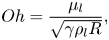 \begin{equation} {Oh}=\frac{\mu_l}{\sqrt{\gamma \rho_{l}R}}, \end{equation}
and measures the relative importance of viscous and inertial forces. The Taylor number:
 \begin{equation} \varGamma= \frac{\varepsilon_{o}E_{c}^{2}R}{\gamma} \end{equation}
measures the relative importance between the electrostatic and capillary stresses. In particular,  $\varGamma = 4$ indicates that the droplet is charged at the Rayleigh limit. The $\varPi _1$ is the ratio between the electrical relaxation time $t_e = \varepsilon _l \varepsilon _o/K_l$ and the characteristic time scale:
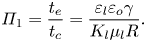 \begin{equation} \varPi_1 = \frac{t_e}{t_c}= \frac{ \varepsilon_l \varepsilon_o \gamma }{K_l\mu_{l} R}. \end{equation}
The  $\varPi _1$ is indicative of the speed at which the charge migrates from the bulk to the surface in an attempt to make the liquid phase equipotential. The dimensionless groups $\varPi _2$, $\varPi _3$ and $\varPi _4$ determine the importance of ion field emission:
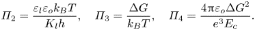 \begin{equation} \varPi_2 = \frac{\varepsilon_l \varepsilon_o k_{B}T }{ K_l h}, \quad \varPi_3 = \frac{\Delta G }{k_{B}T}, \quad \varPi_4 = \frac{4{\rm \pi}\varepsilon_{o}{\Delta G}^{2}}{e^3 E_{c}}. \end{equation}
Here,  $\varPi _2$ is the ratio between the electrical relaxation time and the molecular evaporation time $h/k_B T$, $\varPi _3$ is the ratio between the ion solvation energy and the molecular thermal energy and $\varPi _4$ is the dimensionless characteristic electric field for ion emission, $\tilde {E}^{*}$. Finally, the Péclet number measures the relative importance of convection and diffusion in the Cahn–Hilliard equation:
 \begin{equation} {Pe}=\frac{R^3}{\zeta\gamma t_c}. \end{equation}
For all the numerical cases considered in this study, we make  $\zeta =(R\xi )^{2}/p_{c}t_c$ (Ding, Gilani & Spelt Reference Ding, Gilani and Spelt2010; Mandal et al. Reference Mandal, Ghosh, Bandopadhyay and Chakraborty2015), i.e. ${Pe}=1/\tilde {\xi }^2$.
2.2. Numerical implementation
Our goal is to study the role of ion field evaporation in the formation of electrosprayed nanodroplets of highly conducting liquids, in particular ionic liquids. To the best of our knowledge, this is the only practical situation in which droplets directly form both above the Rayleigh limit and can field emit ions. The central problem is understanding how ion field emission modifies the sprays of a given liquid at varying flow rate, or equivalently as a function of the droplet radius. We focus on the electrosprays of the ionic liquid EMI-Im because it has been thoroughly studied, e.g. it is known that ion emitted from droplets in flight is a key element of the physics, and that some droplets undergo Coulomb explosions while others emit ions and do not fragment (Gamero-Castaño & Cisquella-Serra Reference Gamero-Castaño and Cisquella-Serra2020). Thus, in all calculations, we use the physical properties of EMI-Im,  $\varepsilon _{l}=12.2$, $\rho _{l}=1520\,{\rm kg}\,{\rm m}^{-3}$, $\mu _{l}=0.032\,{\rm Pa}\,{\rm s}$, $K_{l}=0.74\,{\rm S}\,{\rm m}^{-1}$ and $\gamma =0.0349\,{\rm N}\,{\rm m}^{-1}$. For the gas phase, we use $\varepsilon _{g}=1$, $\rho _{g}=1\,{\rm kg}\,{\rm m}^{-3}$, $\mu _{g}= 10^{-4}\,{\rm Pa}\,{\rm s}$ and $K_{g}=10^{-9}\,{\rm S}\,{\rm m}^{-1}$. A precise value of the ion solvation energy is not available and we use the estimate $\Delta G = 1.62$ eV (Iribarne & Thomson Reference Iribarne and Thomson1976; Loscertales & Fernández De La Mora Reference Loscertales and Fernández De La Mora1995; Gamero-Castaño & Fernández De La Mora Reference Gamero-Castaño and Fernández De La Mora2000a). In all simulations, we consider an initial charge $4\,\%$ above the Rayleigh limit, $Q_o=1.04Q_{Ray}$.
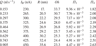
Table 1 shows typical flow rates, beam currents and droplet radii of EMI-Im electrosprays (Gamero-Castaño & Cisquella-Serra Reference Gamero-Castaño and Cisquella-Serra2020), together with the values of size-dependent dimensionless numbers (we assume a charge  $4\,\%$ above the Rayleigh limit). The values of the dimensionless numbers that do not depend on the radius of the droplet are $\varGamma = 4.016$, $\varPi _2 = 906$, $\varPi _3 = 63.1$, $\varepsilon _{l}=12.2$ and ${Pe} = 10^4$ (we use $\xi = R/100$ in all calculations). Note that ion field emission from droplets of highly conducting liquids is characterized by high Ohnesorge numbers (all ionic liquids have high viscosities, comparable or larger to that of EMI-Im, and the droplet radii must be at most a few tens of nanometres to sustain the electric fields needed for significant ion emission) and small $\varPi _1$ (the charge is, for all purposes, relaxed on the surface). Therefore, varying the droplet radius for a given ionic liquid at constant excess charge over the Rayleigh limit is equivalent to varying $\varPi _4$ while keeping $\varGamma$, $\varPi _2$, $\varPi _3$, ${Pe}$ and $\varepsilon _{l}$ constant, in the limit ${Oh}^2 \gg 1$ and $\varPi _1 \ll 1$.
Table 1. Flow rates, beam currents and droplet radii of EMI-Im electrosprays (Gamero-Castaño & Cisquella-Serra Reference Gamero-Castaño and Cisquella-Serra2020), together with size-dependent dimensionless numbers for droplets charged  $4\,\%$ above the Rayleigh limit.
We use COMSOL Multiphysics Software to solve the system of equations (Comsol, Inc. 2019). We employ for most equations COMSOL's built-in laminar flow, electrostatics and phase field interface, which uses a finite element solver. The volumetric charge conservation equation (2.8) cannot be incorporated with built-in interfaces so we use instead the partial differential equation interface. Additionally, we include the electrostatic (2.11) and surface tension (2.12) volumetric forces in (2.7) as forcing terms. The equations are solved in COMSOL's weak formulation framework. The phase variable  $\phi$ is discretized using a cubic-order Lagrange element; $\boldsymbol {u}$, $V$ and $\rho _{e}$ are discretized using quadratic-order Lagrange elements; and $p$ is discretized using a linear Lagrange element. We use the parallel sparse solver MUMPS for marching the solution in time. MUMPS uses a second-order backward differential formulation scheme with variable time step, computed using the Courant–Friedrichs–Lewy condition (Courant, Friedrichs & Lewy Reference Courant, Friedrichs and Lewy1967). The maximum time step is set at $\Delta t_{max}/t_{c}=0.01$, while typical time steps at the start of the simulation are of the order of $10^{-5}$. When needed (e.g. to analyse the results), the position of the surface is computed as the loci where $\phi =0$ by interpolation. For spatial discretization, we use a triangular grid with grid size $h$. The computational domain is divided into two regions, as depicted in figure 2. Region A contains the droplet and its grid size is $h=R/64$, while region B has a grid size $h=R/30$. The variation of the phase variable $\phi$ is depicted in figure 2 along with details of the triangular grid. The diffuse interface thickness is fixed at $\xi =R/100$ (Misra & Gamero-Castaño Reference Misra and Gamero-Castaño2022). The post-processing of the results is performed with the COMSOL–MATLAB interface.
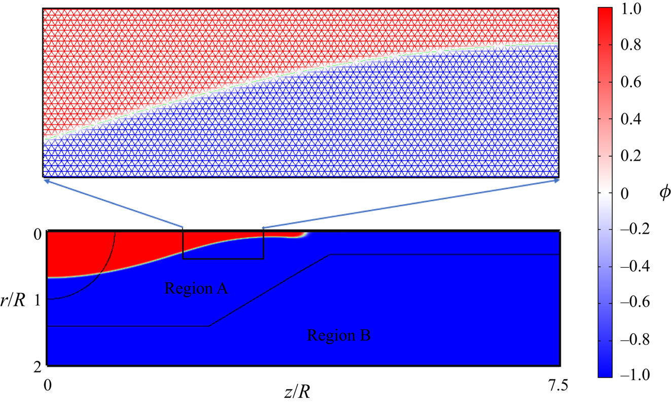
Figure 2. A section of the computational domain along with details of the grid and the variation of the phase variable  $\phi$.
Initially, we impose a homogeneous charge density  $\rho _{e,o}=3 \eta Q_{Ray}/(4 {\rm \pi}R^{3})$ in $\varOmega _l$, with $\eta =1.04$. The charge is allowed to relax at zero fluid velocity, migrating to the interface to make the droplet equipotential (Misra & Gamero-Castaño Reference Misra and Gamero-Castaño2022). Once the charge relaxes, we compute the deformation of the droplet over time. In most calculations, we use $H=L=10R$ and have verified that these values do not affect the solution. When calculating the elongation of the jet, we use a longer domain with $H=14R$. Appendix B provides details about the charge relaxation step and Appendix C presents a grid independence study.
3. Results and discussions
3.1. The Coulomb explosion of a droplet in the absence of ion field emission
This problem has been thoroughly investigated (Burton & Taborek Reference Burton and Taborek2011; Collins et al. Reference Collins, Sambath, Harris and Basaran2013; Garzon et al. Reference Garzon, Gray and Sethian2014; Gawande et al. Reference Gawande, Mayya and Thaokar2017) and the comparison with our solution makes it possible to validate the numerical model. In the remainder of the paper, this case is referred to as ‘pure Rayleigh fission’, PRF. Physically, this scenario corresponds to large droplets with electric fields substantially lower than  $E^{*}$. For the calculations, we use a droplet with $D=50$ nm having the physical properties of EMI-Im, with the exception of using a lower electrical conductivity, $K=0.095\,{\rm S}\,{\rm m}^{-1}$, to simplify capturing the evolution. This leads to $Oh\sim 28$ and $\varPi _{1}\sim 0.05$.
Figure 3(a) shows the evolution of a droplet with  $Q_{o}=1.04Q_{Ray}$. Initially nearly spherical, the droplet becomes an ellipsoid of increasing aspect ratio. The vertices eventually transition into cusps, which elongate to form jets. We quantify the evolution of the droplet with the aspect ratio, ${\it AR}$, defined as the quotient between the spans of the droplet along the axial and radial directions. Figure 3(b) shows the aspect ratio and the electric field on the vertices $\tilde {E}_{tip}$, as a function of time. The shape of the droplet just prior to the formation of jets is referred to as the critical shape. Its aspect ratio, ${\it AR} \cong 3.82$, is close to the experimental value of $3.7\unicode{x2013}3.85$ for droplets in the Stokes limit (Duft et al. Reference Duft, Achtzehn, Müller, Huber and Leisner2003; Achtzehn et al. Reference Achtzehn, Müller, Duft and Leisner2005; Giglio et al. Reference Giglio, Gervais, Rangama, Manil, Huber, Duft, Müller, Leisner and Guet2008); it also compares well with the values of previous numerical calculations, $3.85\unicode{x2013}3.87$ (Gawande et al. Reference Gawande, Mayya and Thaokar2017, Reference Gawande, Mayya and Thaokar2020; Giglio et al. Reference Giglio, Rangama, Guillous and Le Cornu2020). Here, $\tilde {E}_{tip}$ reaches its maximum value for an aspect ratio slightly larger than that of the critical shape. The aspect ratio grows rapidly once the jet is formed. Appendix A provides additional comparison with experimental data.
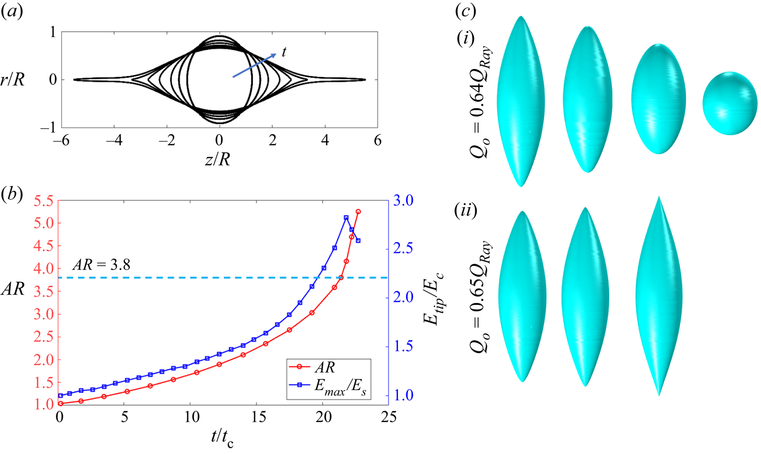
Figure 3. Coulomb explosion of a droplet without ion emission (PRF), with initial charge  $1.04Q_{Ray}$, $Oh=28$ and $\varPi _{1}=0.05$: (a) evolution of the droplet's shape with time. The aspect ratios ( ${\it AR}$) are $1.36$, $1.89$, $2.43$, $3.20$, $3.79$, $4.79$ and $8.41$ at increasing time; (b) evolution of the aspect ratio and the electric field on vertex $\tilde {E}_{tip}$; (c) evolution of the droplet starting right before the critical shape is formed ( ${\it AR}=3.68$), when the total charge is reduced to (c i) $Q_{o}=0.64Q_{Ray}$ and (c ii) $Q_{o}=0.65Q_{Ray}$.
Prior experiments and calculations have shown that the jets are unstable and generate small droplets. The main elongated drop left after the detachment of the progenies relaxes back to a spherical shape, with a charge that is substantially smaller than the original and most of the original mass (Duft et al. Reference Duft, Achtzehn, Müller, Huber and Leisner2003; Giglio et al. Reference Giglio, Gervais, Rangama, Manil, Huber, Duft, Müller, Leisner and Guet2008). An accurate calculation of the dynamics of the jet breakup and the formation of droplet progenies requires a higher grid resolution than employed in this article (the capture of radial features is limited by our choice of interface thickness,  $\xi =R/100$), but doing so increases the computational cost dramatically. Although we do not capture the entire fission process, we can estimate the amount of charge that a parent droplet must shed to become stable. Starting with the shape at ${\it AR}=3.68$ (just prior to the formation of the critical shape), we progressively reduce the charge and observe the evolution to discern whether the droplet develops the jets or goes back to the spherical shape. Figure 3(c) illustrates this approach: starting with a shape ${\it AR}=3.68$, if the charge is made to be $Q_{o}=0.65Q_{Ray}$, the droplet still forms a jet and is unstable. Conversely, if the charge is slightly reduced to $Q_{o}=0.64Q_{Ray}$, the aspect ratio of the droplet decreases and it becomes spheroidal. This suggests that a droplet charged at the Rayleigh limit will shed $36\,\%$ of its charge in a Coulomb explosion. Duft et al. (Reference Duft, Achtzehn, Müller, Huber and Leisner2003) and Giglio et al. (Reference Giglio, Gervais, Rangama, Manil, Huber, Duft, Müller, Leisner and Guet2008) report an experimental charge loss of $33\,\%$, which is in good agreement with our prediction. A recent equipotential model predicts a charge loss of roughly $39\,\%$ (Gawande et al. Reference Gawande, Mayya and Thaokar2017). There is a variation of the fraction of lost charge reported in the literature, which is likely due to viscosity and conductivity effects. For example, for low viscous de-ionized water droplets ( $Oh=0.023$), the critical shape is achieved at ${\it AR}=2.7\unicode{x2013}2.9$ and a charge loss of roughly $20\,\%$ has been measured (Giglio et al. Reference Giglio, Rangama, Guillous and Le Cornu2020), whereas experiments in the Stokes limit ( $Oh\gg 1$) report a charge loss of $33\,\%$ (Duft et al. Reference Duft, Achtzehn, Müller, Huber and Leisner2003; Achtzehn et al. Reference Achtzehn, Müller, Duft and Leisner2005; Giglio et al. Reference Giglio, Gervais, Rangama, Manil, Huber, Duft, Müller, Leisner and Guet2008).
3.2. Droplet charged above the Rayleigh limit with ion field emission
The simulation of a droplet charged above the Rayleigh limit including ion field emission (labelled as WFE, ‘with field emission’) is motivated by the experimental studies of Gamero-Castaño & Cisquella-Serra (Reference Gamero-Castaño and Cisquella-Serra2020), Miller et al. (Reference Miller, Ulibarri-Sanchez, Prince and Bemish2021) and Perez-Lorenzo & Fernández De La Mora (Reference Perez-Lorenzo and Fernández De La Mora2022), who report substantial ion currents in electrosprays of several ionic liquids. Retarding potential measurements indicate that these ions are emitted from droplets likely to be charged above the Rayleigh limit. Our simulations reveal three distinct outcomes depending on the initial size of the droplet.
3.2.1. Small radius regime, region  $I$
$I$

Sufficiently small droplets charged above the Rayleigh limit emit ions from the spherical and spheroidal shapes. Figure 4 shows the evolution of droplets with diameters of 10 and 20 nm charged  $4\,\%$ above the Rayleigh limit. The 10 nm droplet undergoes marginal deformation while emitting ions, before becoming a stable sphere. The $20$ nm droplet follows a similar path, but undergoes a larger deformation. In either case, the droplet does not develop the cusps preceding the formation of the jets and droplet progenies, i.e. the shedding of charge by ion field emission prevents the Coulomb explosion.
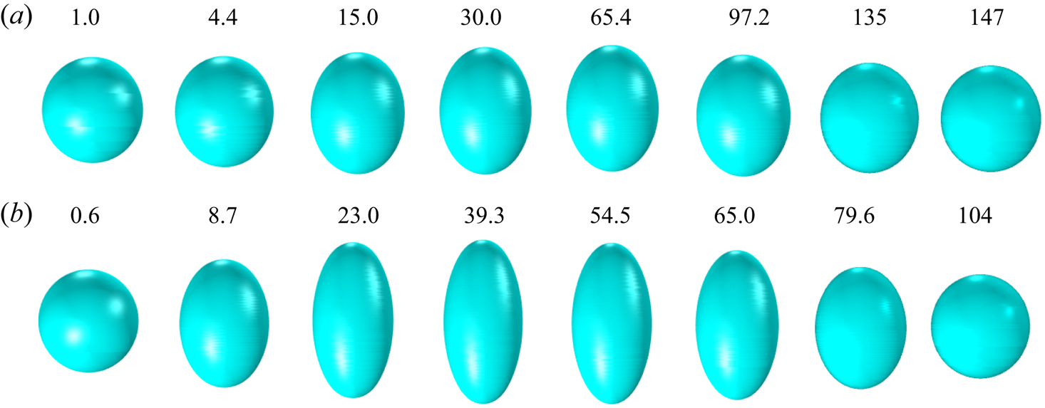
Figure 4. Evolution of EMI-Im droplets emitting ions, with an initial charge  $Q_{o}= 1.04Q_{Ray}$: (a) $D = 10\,{\rm nm}$; (b) $D = 20\,{\rm nm}$. The times $t/t_{c}$ for each snapshot are shown above the drops.
Figure 5(a) shows the charge of three ion-emitting droplets with diameters of  $10$,
$10$,  $15$ and $20$ nm as a function of time, while figure 5(b) shows their aspect ratios together with that of a $50$ nm droplet in the PRF regime (without ion emission). The initial charge of all droplets is $4\,\%$ above the Rayleigh limit. The characteristic time for the shedding of charge scales with $t_c$, while the fraction of the initial charge that is evaporated increases with decreasing droplet diameter. This is to be expected from the dependency of the electric field on the diameter of a droplet at the Rayleigh limit, (1.1a,b). Note that as the droplets emit ions, their aspect ratios increase. The droplets remain quasi-equipotential during the deformation, and the electric field on the surface scales with the inverse of the square of the local radius of curvature. Thus, as the aspect ratio of the droplet increases, ion emission preferentially takes place from the vertices of the ellipsoid. The aspect ratios of the droplets plateau once ion emission becomes negligible, a larger droplet exhibits a larger deformation. From this state of maximum deformation, the droplet falls back to the spherical shape, now stable with a constant charge that can be significantly smaller than the Rayleigh limit. The 10, 15 and 20 nm droplets lose $38\,\%$, $28\,\%$ and $20\,\%$ of their initial charge, respectively. Given the substantial charge loss, the electric stress at the vertices of the ellipsoid is insufficient to form the cusps and jets characteristic of a Coulomb explosion.
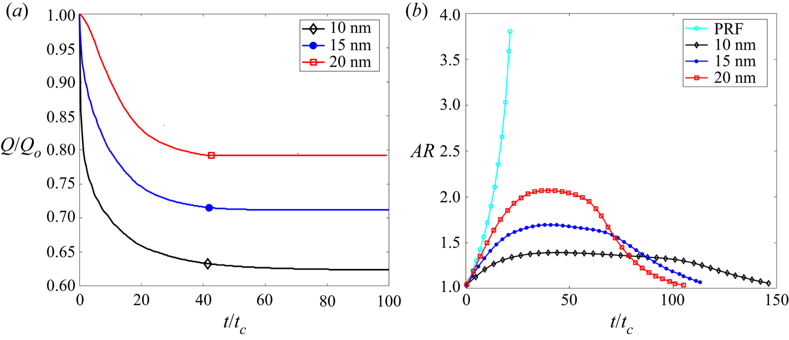
Figure 5. EMI-Im droplets with different diameters emitting ions (initial charge  $Q_{o}= 1.04Q_{Ray}$): (a) evolution of the charge held by the droplet; (b) evolution of the aspect ratio and comparison with that of a droplet in the PRF regime (without ion emission).
Figure 6 shows the evolution of the normal component of the electric field at the vertex of the droplet. In all cases, the electric field levels off near  $E_{n}^{g}/E^{*} \approx 0.76$ when ion emission is significant, i.e. $0.76\times E^{*}$ is the effective value of the electric field during ion emission: when the electric field is slightly above $0.76\times E^{*}$, the high intensity of the ion flux (see exponential dependency of the emitted current on the electric field) rapidly reduces the charge of the droplet, bringing down the electric field to this effective value for ion emission; and ion emission is negligible if the electric field is slightly below $0.76\times E^{*}$. The initial electric field for the two smaller droplets is above the effective value and therefore both of them are characterized by an initial brief period of intense ion emission. Conversely, the electric field for the larger droplet, $D = 20$ nm, is initially below the effective value and, although the droplet emits ions from its initial state, it needs to deform to reach the effective electric field and increase ion emission. The total charge evaporated during the time in which the electric field is approximately constant is significant for all three droplets (see figure 5a). The freezing of the electric field during ion emission was previously observed in the experiments by Loscertales & Fernández De La Mora (Reference Loscertales and Fernández De La Mora1995). Finally, note that the evolution of the electric field in figure 6 may exhibit, at times, an unphysical wiggle. This artefact is due to how we evaluate the electric field for the purpose of making the plot: $E_{n}^{g}$ is defined at the surface, which in general does not coincide with the position of the nodes in the computational grid. Thus, we compute $E_{n}^{g}$ by interpolating the values of the electric field between two nodes, in a region where the electric field and the volumetric charge exhibit large gradients. This causes the wiggle. A more accurate way of computing $E_{n}^{g}$ would consist of using more nodes in the grid to fit the values of the electric field to appropriate analytical functions and determining the value at the surface from the fitting. However, note that this is only important for plotting purposes, because $E_{n}^{g}$ is not a variable used in the calculations (the surface and therefore the electric field at the surface are not part of the calculations in the phase field method).

Figure 6. Evolution of the outer electric field on the vertices of EMI-Im droplets emitting ions, with an initial charge  $Q_{o} = 1.04Q_{Ray}$.
3.2.2. Medium radius regime, region $II$

In this case, the initial electric field on the surface of the spherical droplet is insufficient to emit ions. Similarly to the PRF case, the unstable droplet deforms into an ellipsoid of increasing aspect ratio at constant charge. As the electric field near the vertices of the ellipsoid increases, it eventually becomes high enough to promote significant ion emission, discharging the droplet and preventing the Coulomb explosion.
Figure 7 displays the evolution of a  $D = 30$ nm droplet initially charged $4\,\%$ above the Rayleigh limit. Figure 7(a) shows the droplet deforming into an ellipsoid of increasing aspect ratio, reaching a maximum deformation, and going back to a sphere without developing the cusps and jets typical of a Coulomb explosion. Figure 7(b) shows the aspect ratio, the charge and the electric field at the vertices of the droplet as functions of time. Initially, the trend for the aspect ratio coincides with that for the PRF case because the electric field near the vertices is insufficient to support ion emission. However, as the electric field at the vertices reach a critical value at $t/t_{c}\sim 10$, the droplet begins to shed charge and the aspect ratios of the PRF and WFE droplets start to separate. The aspect ratio of the WFE droplet, rather than accelerating, reaches a maximum at $t/t_{c}\sim 38$. By this time, the droplet has lost $17.3\,\%$ of its charge by ion field emission, which takes place at nearly constant electric field, $E_{n}^{g}/E^{*} \sim 0.76\unicode{x2013}0.77$. Most of the ion emission occurs up to the maximum of the aspect ratio. Minor ion emission continues to take place as the droplet relaxes to the stable spherical configuration, being negligible for $t/t_{c}\gtrsim 54$. Because of the reduced electrification, the cusps and jets never develop, i.e. the Coulomb explosion is suppressed.
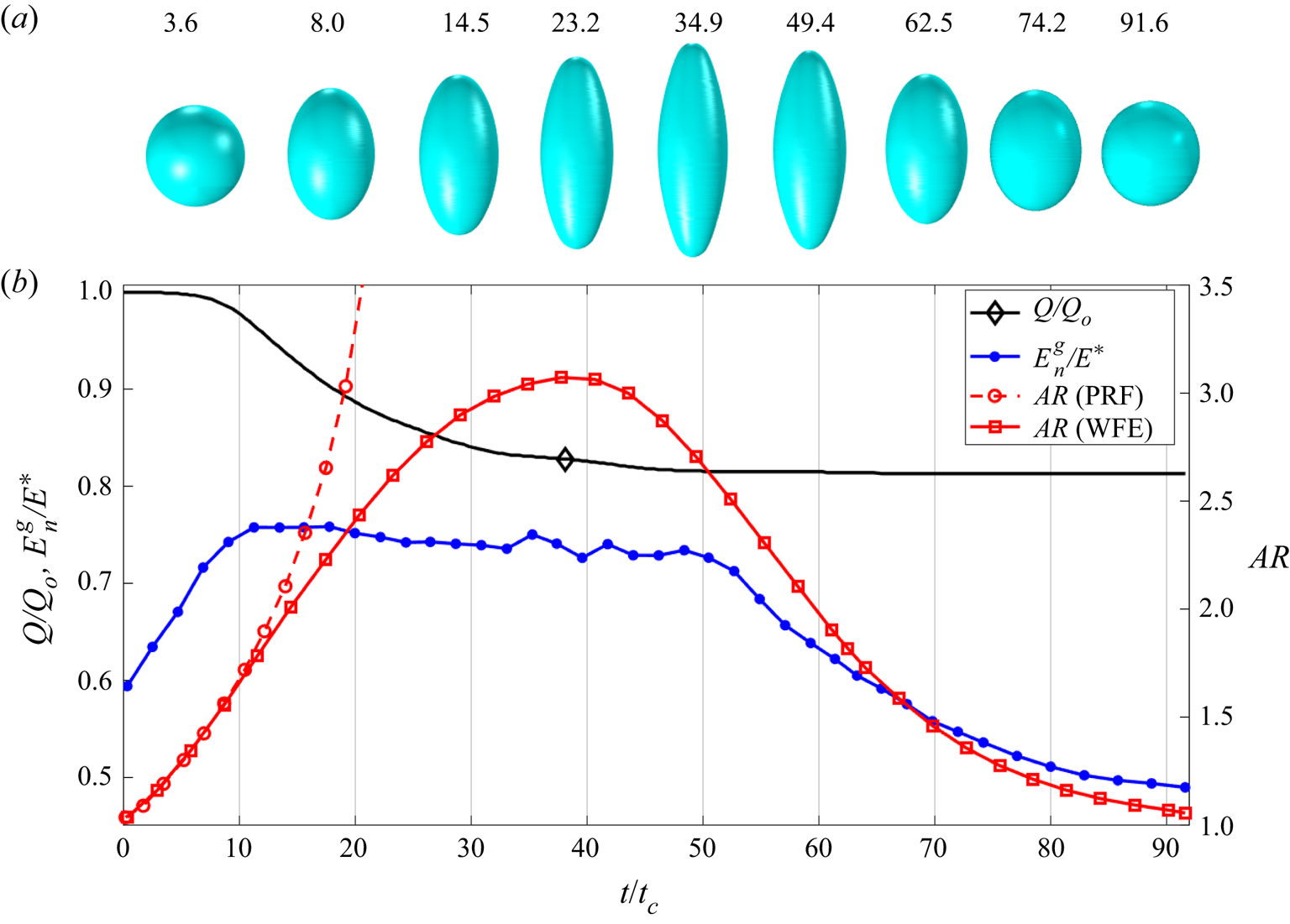
Figure 7. Results for a  $D = 30$ nm droplet with initial charge $Q_{o}=1.04Q_{Ray}$, including ion emission: (a) evolution of the droplet's shape ( $t/t_{c}$ is shown above the drops); (b) evolution of the aspect ratio (for comparison, we also include the aspect ratio of a PRF droplet), charge and outer electric field at the vertices of the droplet.
Figure 8 shows the evolution for a larger droplet,  $D=40$ nm, also charged $4\,\%$ above the Rayleigh limit. Although, in this case, ion emission is triggered at a later time due to the lower initial electric field, it also suppresses the Coulomb explosion. The droplet follows the PRF trend for a longer time due to the later onset of ion emission. At $t/t_{c}\sim 14$, the electric field at the vertices is sufficiently high to trigger ion emission ( $E_{n}^{g}/E^{*}\sim 0.76\unicode{x2013}0.77$). The droplet starts to emit charge and the aspect ratio separates from the PRF droplet. Note that the vertices of the ellipsoid are almost transitioning into cusps when the aspect ratio plateaus at $t/t_{c}\sim 38.2$. Interestingly, the aspect ratio exceeds $3.8$, which is the critical aspect ratio for the PRF case. The larger 40 nm droplet sheds a higher fraction of its initial charge than the $30$ nm droplet, $\sim 24\,\%$ and $\sim 19\,\%$, respectively.
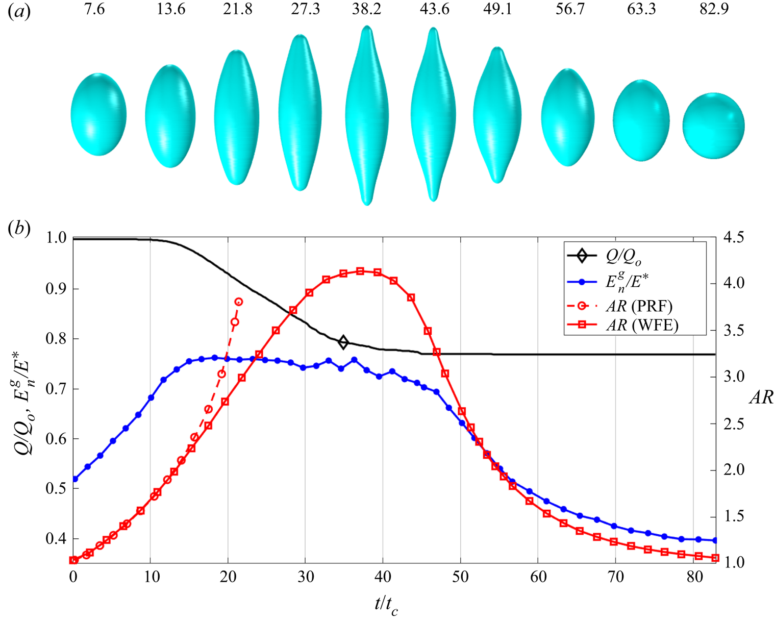
Figure 8. Same as figure 7 for a larger droplet,  $D = 40$ nm.
These findings (regions I and II) provide an alternative scenario for ion emission to that proposed by previous authors who assume that it takes place from a spherical droplet only when its initial electric field  $E_o$ can promote significant ion emission while being lower than that associated with the Rayleigh limit, $E^{*}\leq E_o< E_{Ray}$ (Iribarne & Thomson Reference Iribarne and Thomson1976; Labowsky Reference Labowsky1998; Labowsky et al. Reference Labowsky, Fenn and Fernández De La Mora2000). Furthermore, they confirm the qualitative arguments put forward by Gamero-Castaño & Fernández de la Mora (Reference Gamero-Castaño and Fernández de la Mora2000) and Gamero-Castaño & Cisquella-Serra (Reference Gamero-Castaño and Cisquella-Serra2020), namely that droplets undergoing Coulomb explosions may emit ions from areas of high electric fields, suppressing the fission process.
3.2.3. Large radius regime, region $III$

Lastly, we discuss relatively large droplets charged above the Rayleigh limit, specifically in the diameter range  $45\unicode{x2013}100$ nm. The unstable droplet evolves into an ellipsoid, developing cusps and jets. Ion emission may take place from the vertices and the jets, but cannot prevent the Coulomb explosion. Both ion emission and droplet progenies reduce the charge of the droplet.
Figure 9 shows a simulation for a  $D = 45$ nm droplet initially charged $4\,\%$ above the Rayleigh limit. The evolution of the shape is qualitatively similar to the PRF case: the spherical droplet becomes an ellipsoid of increasing aspect ratio; it develops cusps at the vertices; and the cusps move away from the centre forming jet-like extensions. Ion emission is negligible until $t/t_{c}=15.4$. Beyond this time, the electric field at the vertices is high enough to emit ions, lowering the charge of the droplet and slowing the speed at which the aspect ratio increases. However, the shedding of charge does not impede the formation of cusps and jets, depicted in the droplet profiles at $t/t_{c}= 33.9, 37.8$ and 40.7. It is interesting that electric fields high enough to evaporate ions only develop at the vertices of the spheroid and at the cusps. At $t/t_{c}\gtrsim 38$, the electric field at the cusps is not sufficient to continue the emission of ions and the net charge of the droplet remains constant. The jets continue to elongate, and we assume that natural instability will lead to their breakup and the formation of droplet progenies. Overall, the droplet sheds roughly $28\unicode{x2013}29\,\%$ of its charge by ion emission. Profiles of the electric field along the surface at different times are shown in figure 9(c), $t/t_{c}=35.3$, and figure 9(d), $t/t_{c}=41.2$. At the earlier time, the electric field increases towards the cusps, where it reaches a value consistent with significant ion evaporation, $E_{n}^{g}/E^{*}=0.76\unicode{x2013}0.77$. The profile for $t/t_{c}=41.2$, i.e. for a situation with developed jets, shows two distinct maxima. The lower maximum occurs near the transition region of the jet $z/R\sim 2.6\unicode{x2013}2.7$, whereas the larger electric field occurs at the tip of the jet. The value of the latter is $E_{n}^{g}/E^{*} \sim 0.67$, i.e. insufficient to trigger significant ion emission, as reflected by the constancy of the charge carried by the droplet at this time.
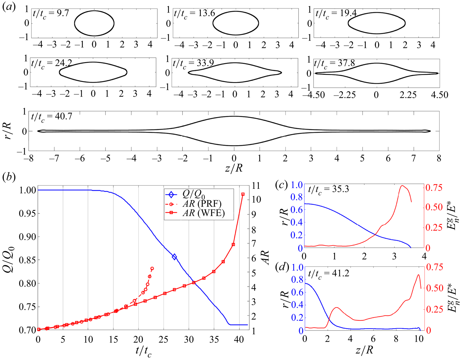
Figure 9. Simulation of a  $D = 45$ nm droplet with initial charge $Q_{o}=1.04Q_{Ray}$, undergoing Coulomb explosion and ion field emission (WFE): (a) droplet shape at different times; (b) evolution of the charge and aspect ratio of the droplet; (c) profile of the droplet's surface and outer electric field at $t/t_{c}=35.3$; (d) profile of the droplet's surface and outer electric field at $t/t_{c}=41.2$.
Figure 10 shows that larger droplets (diameters of 50, 80 and 100 nm) behave similarly to the droplet with a diameter of 45 nm: ion emission is absent from the initial spherical configuration; the deformation follows the PRF path until the electric field at the vertices is sufficient to evaporate ions; and ion emission does not prevent the formation of jets and the Coulomb explosion. The aspect ratio curves match the PRF trend for most of the evolution; however, the three curves depart from the PRF trend before the critical shape forms. This is due to the onset of ion emission from the vertices before the formation of cusps. Larger droplets follow the PRF path more closely and we expect that ion emission never occurs for sufficiently large droplets. The three droplets loose a similar fraction of their charge by ion emission, approximately  $24\,\%$, but the loss is more gradual and starts at an earlier time for the smaller droplet. As in the case of the $D = 45$ nm droplet, ion emission eventually ceases at a time when the jet is still elongating, suggesting that the droplets will undergo Coulomb explosions and produce droplet progenies.
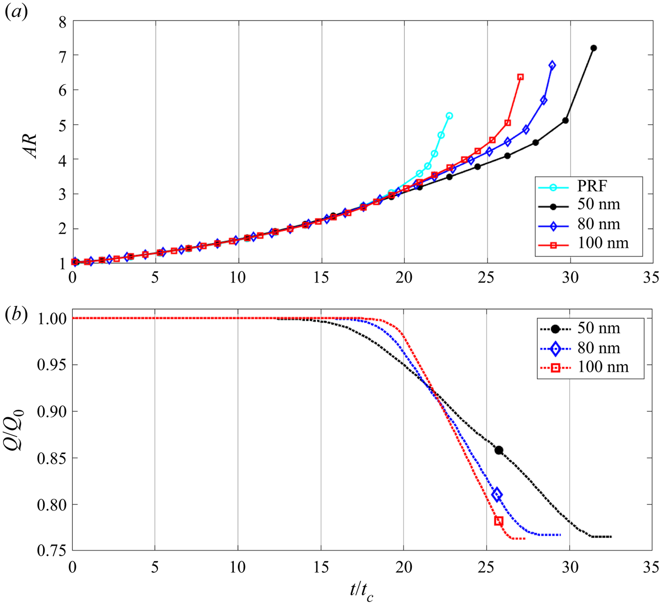
Figure 10. Results for droplets with diameters of 50, 80 and 100 nm: (a) evolution of the aspect ratio and comparison with that of a PRF droplet; (b) evolution of the droplet's charge.
In our calculations, the large droplets that emit ions during a Coulomb explosion lose approximately  $24\,\%$ of their charge by ion emission. Since the total charge loss of PRF droplets is approximately $36\,\%$, we estimate that the droplets in region III lose approximately $16\,\%$ of the charge in the form of droplet progenies (considering that $Q_{o}=1.04Q_{Ray}$). The rationale behind this estimate is that the shape of the ion-emitting droplet at the time the jets form is similar to the critical shape of the PRF droplet and therefore they both must lose a similar amount of charge to fall back to the stable spherical configuration (this is the argument made by figure 3c). The comparison of the droplet shapes shown in figure 11 supports this estimate: the shape of the PRF droplet right before the critical point ( ${\it AR} = 3.68$, see figure 3a) matches the profile of the $D = 100$ nm droplet well, with slight differences near the vertices. Our estimate that large droplets lose approximately $24\,\%$ of their charge by ion emission agrees with the findings of Perez-Lorenzo & Fernández De La Mora (Reference Perez-Lorenzo and Fernández De La Mora2022), who hypothesize that the majority of ions observed in the electrosprays of EMI-FAP are emitted from nanodroplets undergoing Coulomb explosions. The experiments of Perez-Lorenzo & Fernández De La Mora (Reference Perez-Lorenzo and Fernández De La Mora2022) show that approximately $20\unicode{x2013}25\,\%$ of the total current is emitted in the form of ions, a value not far from our prediction; furthermore, the average diameter of the primary droplets of EMI-FAP in these experiments is estimated to be near 90 nm, i.e. within regime III.
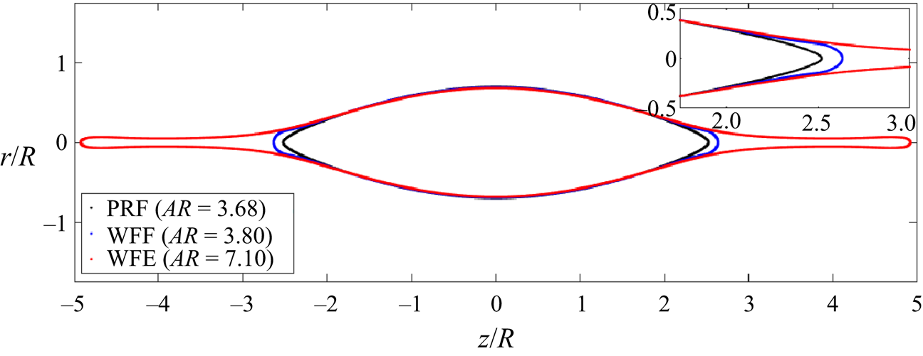
Figure 11. Profiles of a  $D = 100$ nm droplet undergoing Coulomb explosion with ion emission ( ${\it AR}=3.80$ and ${\it AR}=7.10$) and comparison with a PRF droplet near the critical shape ( ${\it AR}=3.68$).
Figure 12(a) shows the total charge emitted from EMI-Im droplets in regions I and II by ion emission as a function of the diameter of the droplet. Figure 12(b) plots the electric field on the surface of a spherical droplet charged 4 % above the Rayleigh limit, as a function of the diameter of the droplet (the electric field is normalized with the characteristic value for ion emission  $E^{*}$); figure 12(b) also shows the domains of regions I, II and III. Here, $E_{c}/E^{*} \gtrsim 0.77$ in region I and, therefore, ion emission is significant from the initial spherical configuration. Although the droplet deforms into an ellipsoid of increasing aspect ratio, ion emission prevents the formation of cusps and the Coulomb explosion and, once enough charge is shed, the droplet goes back to a spherical shape with a charge below the Rayleigh limit. Region II is characterized by droplets with initial electric fields in the range $0.47 \lesssim E_{c}/E^{*} \lesssim 0.77$. The initial electric field is not sufficient to trigger ion emission; however, as the droplet deforms and the curvature at the vertices becomes large enough, ions are emitted from this small region, discharging the droplet and preventing the formation of cusps and the Coulomb explosion. The droplet subsequently retracts to the stable spherical configuration below the Rayleigh limit. Region III is characterized by initial electric fields $E_{c}/E^{*} \lesssim 0.47$. These droplets develop cusps and jets, and hence undergo Coulomb explosions yielding droplet progenies. These droplets lose a significant fraction of their charge by ion emission from their vertices and jets; however, the reduction of charge does not prevent the Coulomb explosion and the formation of droplet progenies.
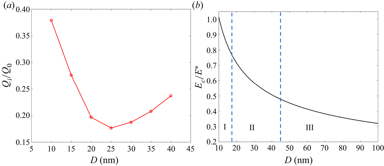
Figure 12. (a) Charge lost by ion emission ( $Q_{i}$) for droplets in regions I and II; (b) electric field on the surface of a spherical droplet charged 4 % above the Rayleigh limit, as a function of the diameter of the droplet and ranges of regions I, II and III.
We can estimate the maximum diameter of the droplet,  $D_{max}$, for which ion emission is significant, i.e. the diameter separating region III from the PRF regime. Figure 3(b) shows that, for EMI-Im droplets in the PRF regime charged near the Rayleigh limit, the maximum value of the electric field, $E_{tip}/E_{Ray} \cong 2.83$, occurs at the cusps when the aspect ratio is slightly larger than that of the critical shape. Furthermore, ion emission is significant only when $E_{max}/E^{*} \geq 0.76$. These two relations can be combined to obtain $D_{max}$ (considering droplets $4\,\%$ above the Rayleigh limit):
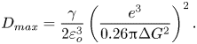 \begin{equation} D_{max}=\frac{\gamma}{2 \varepsilon_{o}^3} \left( \frac{e^3}{0.26 {\rm \pi}\Delta G^2} \right) ^2. \end{equation}
Here,  $D_{max} = 140$ nm for the conditions used in our numerical calculations. We expect droplets with larger diameters to be in the PRF regime.
We have used an initial charge  $4\,\%$ over the Rayleigh limit or equivalently, $\varGamma = 4.016$, in all simulations. A higher initial charge excess should have a minor effect on the size windows of regions I, II and III because although ions would be emitted earlier during the deformation of the droplet, the exponential nature of the ion emission law fixes the maximum electric field at a precise fraction of $E^*$. The amount of charge emitted from a droplet of a given radius with initial charge $\eta Q_{Ray}$ will increase with the initial charge and should approximately be that of the droplet charged $4\,\%$ over the Rayleigh limit plus $(\eta -1.04)Q_{Ray}$. Furthermore, using a small charge excess over the Rayleigh limit is representative of practical conditions: for example, charged droplets in aerosols reach the Rayleigh limit by evaporation of the liquid phase at constant charge, i.e. $Q_o/Q_{Ray}$ increases towards 1; and the charged nanodroplets produced during the jet breakup of an electrospray are, at most, slightly charged above the Rayleigh limit, because the breakup process distributes the charge and mass of the jet among neighbouring droplets to minimize the excess charge (Misra & Gamero-Castaño Reference Misra and Gamero-Castaño2022).
4. Conclusions
We have developed an electrohydrodynamic phase field model to study the coupling of ion emission and Coulomb explosion in charged liquid droplets. The model accounts for the finite electric conductivity of the liquid. We draw the following major conclusions from the current study.
(i) Highly viscous droplets charged slightly above the Rayleigh limit emit roughly
$36\,\%$ of their charge in the form of smaller droplet progenies. This analysis does not take into account ion field emission and, therefore, is valid for relatively large droplets where the electric field on the surface is not sufficient to support ion emission. For the EMI-Im droplets and conditions considered in the current article, we expect droplets with diameter $D > 140$ nm to follow this trend.(ii) Ion field emission suppresses Coulomb explosions in droplets that are charged above the Rayleigh limit and are sufficiently small (
$D < 45$ nm in our simulations with EMI-Im droplets). Between $20\text { and }40\,\%$ of the initial charge of the droplet is shed by ion emission (we assume an initial charge $4\,\%$ above the Rayleigh limit).(iii) There is an intermediate size range (
$45 \lesssim D \lesssim 100$ nm in our simulations with EMI-Im droplets) in which droplets charged above the Rayleigh limit undergo Coulomb explosions, and also emit ions from the vertices and jets of the deforming droplet. We find that approximately $24\,\%$ of the initial charge of the droplet is shed by ion emission and estimate that roughly $15\unicode{x2013}16\,\%$ is lost in the form of droplet progenies. This prediction matches well the experiments and analysis of Perez-Lorenzo & Fernández De La Mora (Reference Perez-Lorenzo and Fernández De La Mora2022).(iv) Ion emission freezes the value of the electric field in areas where emission is significant. We quantify this value at
$E_{n}^{g}/E^{*}\sim 0.76\unicode{x2013}0.77$.


The continuum approach and the leaky dielectric model have been successful in reproducing Coulomb explosions in the past (Giglio et al. Reference Giglio, Gervais, Rangama, Manil, Huber, Duft, Müller, Leisner and Guet2008; Gawande et al. Reference Gawande, Mayya and Thaokar2017, Reference Gawande, Mayya and Thaokar2020; Giglio et al. Reference Giglio, Rangama, Guillous and Le Cornu2020). However, these prior studies compare numerical results with experimental data for droplets 10–50  $\mathrm {\mu }{\rm m}$ in diameter (Duft et al. Reference Duft, Achtzehn, Müller, Huber and Leisner2003; Achtzehn et al. Reference Achtzehn, Müller, Duft and Leisner2005; Giglio et al. Reference Giglio, Gervais, Rangama, Manil, Huber, Duft, Müller, Leisner and Guet2008). Ion emission is relevant only in nanometric droplets and, in these systems, the continuum approximation as well as key assumptions of the leaky dielectric model such as constant electrical conductivity may be less accurate. However, we note that molecular dynamic simulations of ion emission and Coulomb explosions in droplets with diameter less than $10$ nm (Luedtke et al. Reference Luedtke, Landman, Chiu, Levandier, Dressler, Sok and Gordon2008) show good qualitative agreement with our calculations. Moreover, recent continuum studies of ion emission from Taylor cones provide confidence in our treatment of this problem (Higuera Reference Higuera2008; Coffman et al. Reference Coffman, Martínez-Sánchez, Higuera and Lozano2016, Reference Coffman, Martínez-Sánchez and Lozano2019; Gallud & Lozano Reference Gallud and Lozano2022). Regarding the validity of the leaky dielectric model, it has been shown that this formulation accurately reproduces the similar problem of cone-jets (Gamero-Castaño & Magnani Reference Gamero-Castaño and Magnani2019). However, we plan to improve the present model by using an electrokinetic formulation, thus relaxing the assumption of a constant electrical conductivity.
Acknowledgment
K.M. would like to thank M. Magnani for several useful suggestions regarding the numerical set-up and results.
Funding
This work was funded by the Air Force Office of Scientific Research, Award No. FA9550-21-1-0200; we thank the monitor of the program Dr M. Birkan for his support. K.M. would also like to acknowledge the Science and Engineering Research Board (SERB), DST India, for partial financial support.
Declaration of interests
The authors report no conflict of interest.
Appendix A. Additional validation of Coulomb explosion calculation
Figure 13 shows a comparison between the actual shape of an ethylene glycol droplet undergoing a Coulomb explosion (second snapshot of figure 4 in Achtzehn et al. Reference Achtzehn, Müller, Duft and Leisner2005) ( $Oh>1$) and the critical shape computed with the model ( $Oh=28$, $\varPi _{1}=0.05$). ImageJ software was used to extract the experimental profile (Abràmoff, Magalhães & Ram Reference Abràmoff, Magalhães and Ram2019; Misra Reference Misra2020). The resolution of the image of Achtzehn et al. (Reference Achtzehn, Müller, Duft and Leisner2005) is not high enough to accurately extract the profile of the jet emitted from the vertex. The comparison shows good agreement between the numerical and experimental profiles, and a good prediction of the critical aspect ratio. The computed semi-cone angle is between $26^{\circ }\text { and }28.5^{\circ }$ for times near the formation of the critical shape, in agreement with prior numerical results (Betelú et al. Reference Betelú, Fontelos, Kindelán and Vantzos2006; Fontelos, Kindelán & Vantzos Reference Fontelos, Kindelán and Vantzos2008; Gawande et al. Reference Gawande, Mayya and Thaokar2017; Wang, Ma & Siegel Reference Wang, Ma and Siegel2019; Gawande et al. Reference Gawande, Mayya and Thaokar2020) and values near $30^{\circ }$ observed in experiments (Duft et al. Reference Duft, Achtzehn, Müller, Huber and Leisner2003; Achtzehn et al. Reference Achtzehn, Müller, Duft and Leisner2005; Giglio et al. Reference Giglio, Gervais, Rangama, Manil, Huber, Duft, Müller, Leisner and Guet2008).
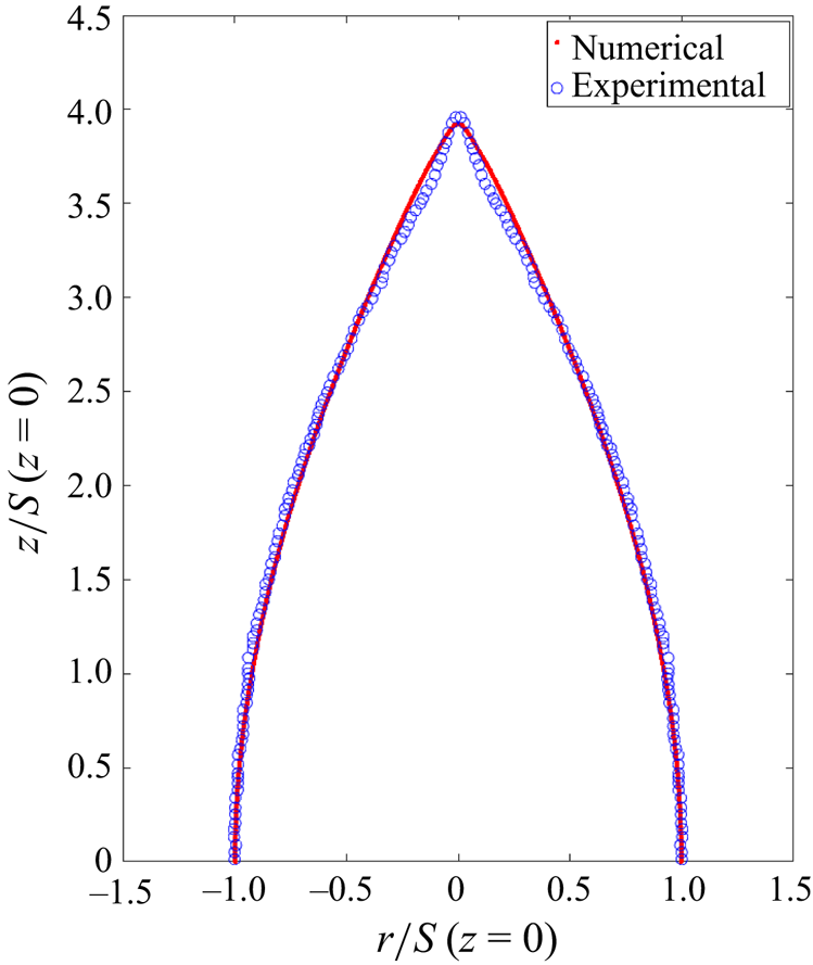
Figure 13. Comparison between the critical shapes of droplets: computed with the model (red) and experimental profile for an ethylene glycol droplet undergoing a Coulomb explosion reported by Achtzehn et al. (Reference Achtzehn, Müller, Duft and Leisner2005) (blue circles).
Perfectly conducting droplets form a conical singularity at the vertices due to the absence of tangential electric stress (Betelú et al. Reference Betelú, Fontelos, Kindelán and Vantzos2006; Fontelos et al. Reference Fontelos, Kindelán and Vantzos2008; Gawande et al. Reference Gawande, Mayya and Thaokar2017). The formation of a conical singularity in perfectly conducting droplets is self-similar with the tip curvature and tip velocity scaling as  $l_{c}\kappa _{tip}={O}(\tau ^{-\alpha })$ and $w_{tip}/u_{c}={O}(\tau ^{\alpha -1})$, respectively, where $l_{c}\kappa _{tip}$, $w_{tip}/u_{c}$ are the dimensionless curvature and axial velocity of the tip (Fontelos et al. Reference Fontelos, Kindelán and Vantzos2008), and $\tau =(t_{s}-t)/t_{c}$ is the dimensionless time to singularity formation (at $t=t_{s}$, singularity occurs). While the singularity never arises in droplets with finite conductivity, Wang et al. (Reference Wang, Ma and Siegel2019) realized that if the scaling laws for perfectly conducting droplets are true, then $\tau \sim 1/t_{c}\kappa _{tip}w_{tip}$. Since $w_{tip}$ and $\kappa _{tip}$ are accurately determined from the simulation, we can have a prediction for $\tau$, and use the numerical solution to compare the scalings for the tip curvature and the velocity near the formation of the critical shape in droplets with finite electrical conductivity.
Figure 14(a,b) depict the dimensionless tip curvature and axial velocity respectively for  $Oh=28$ and $\varPi _{1}=0.004$. The last time stamp in these plots coincides with the critical shape depicted in figure 13. Figure 14(c) depicts the tip curvature and velocity as functions of $1/t_{c}\kappa _{tip}w_{tip}$, similarly to the analysis by Wang et al. (Reference Wang, Ma and Siegel2019). The asymptotes are also fitted for each of the cases near the formation of critical shape. The fitting yields $\alpha \sim 0.7\unicode{x2013}0.71$. Interestingly, Fontelos et al. (Reference Fontelos, Kindelán and Vantzos2008) find $\alpha \sim 0.72$ for conducting droplets in the presence of an external electric field (the semi-cone angle in this case is $27.5^{\circ }$). Wang et al. (Reference Wang, Ma and Siegel2019) obtained $\alpha =0.71$ and a semi-cone angle of $21^{\circ }\unicode{x2013}24^{\circ }$ with an electrokinetic model.
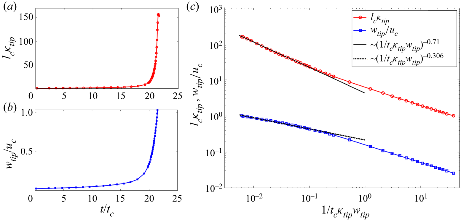
Figure 14. Results for  $Oh=28$, $\varPi _{1}=0.05$: (a) dimensionless tip curvature $l_{c}\kappa _{tip}$ as a function of time; (b) tip velocity $w_{tip}/u_{c}$ as a function of time; (c) variation of $l_{c}\kappa _{tip}$ and $w_{tip}/u_{c}$ with $1/t_{c}\kappa _{tip}w_{tip}$.
Appendix B. Charge relaxation and jump of the electric field across the surface
We next compare the numerical and analytical solutions for the relaxation of an initial homogeneous volumetric charge density  $\rho _{eo}$ in the droplet. The migration of charge in the bulk is governed by the charge conservation equation:
 \begin{equation} \frac{\partial \rho_e}{\partial t} + \boldsymbol{\nabla} \boldsymbol{\cdot} (\rho_{e}\boldsymbol{u})={-}\boldsymbol{\nabla}\boldsymbol{\cdot}(K\boldsymbol{E}), \end{equation}
which can be derived starting from the Poisson–Nernst–Planck (PNP) equation for charged species (Saville Reference Saville1997) and assuming constant electrical conductivity, negligible diffusion current and fully dissociated salts. For further details of this derivation, see Saville (Reference Saville1997), Herrada et al. (Reference Herrada, López-Herrera, Gañán-Calvo, Vega, Montanero and Popinet2012) and Gañán-Calvo et al. (Reference Gañán-Calvo, López-Herrera, Herrada, Ramos and Montanero2018); an excellent discussion of its assumption is provided by Ganán-Calvo et al. (Reference Ganán-Calvo, López-Herrera, Rebollo-Munoz and Montanero2016).
Assuming constant electrical conductivity and zero velocity, the charge conservation equation simplifies to
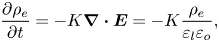 \begin{equation} \frac{\partial \rho_e}{\partial t}={-}K\boldsymbol{\nabla}\boldsymbol{\cdot}\boldsymbol{E} ={-}K\frac{\rho_{e}}{\varepsilon_{l}\varepsilon_{o}}, \end{equation}
and the charge density is given by
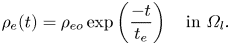 \begin{equation} \rho_e(t)=\rho_{eo}\exp\left(\frac{-t}{t_{e}}\right) \quad \text{in}\ \varOmega_l. \end{equation}
When the charge has fully migrated to the surface, the droplet is equipotential and the electric field is given by
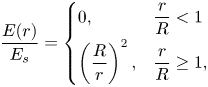 \begin{equation} \frac{E(r)}{E_s} =
\left\{ \begin{array}{@{}ll} 0, & \dfrac{r}{R} < 1 \\
\left(\dfrac{R}{r}\right)^{2}, & \dfrac{r}{R} \ge 1, \end{array} \right.
\end{equation}
\begin{equation} \frac{E(r)}{E_s} =
\left\{ \begin{array}{@{}ll} 0, & \dfrac{r}{R} < 1 \\
\left(\dfrac{R}{r}\right)^{2}, & \dfrac{r}{R} \ge 1, \end{array} \right.
\end{equation}
where  $r$ is the radial spherical coordinate and $E_{s}=Q/(4{\rm \pi} \varepsilon _{o}R^{2})$ is the electric field on the surface of the droplet.
Figure 15(a) shows the decay of the volumetric charge density inside the droplet computed both analytically and with the model. Figure 15(b) shows the spatial variation of the electric field once the charge has relaxed to the surface, both computed with the model and (B4). The inset shows the variation of the volumetric charge. While the phase field method relies on the continuous variation of the phase variable ( $\phi$), the method accurately captures the jump in the electric field across the surface.
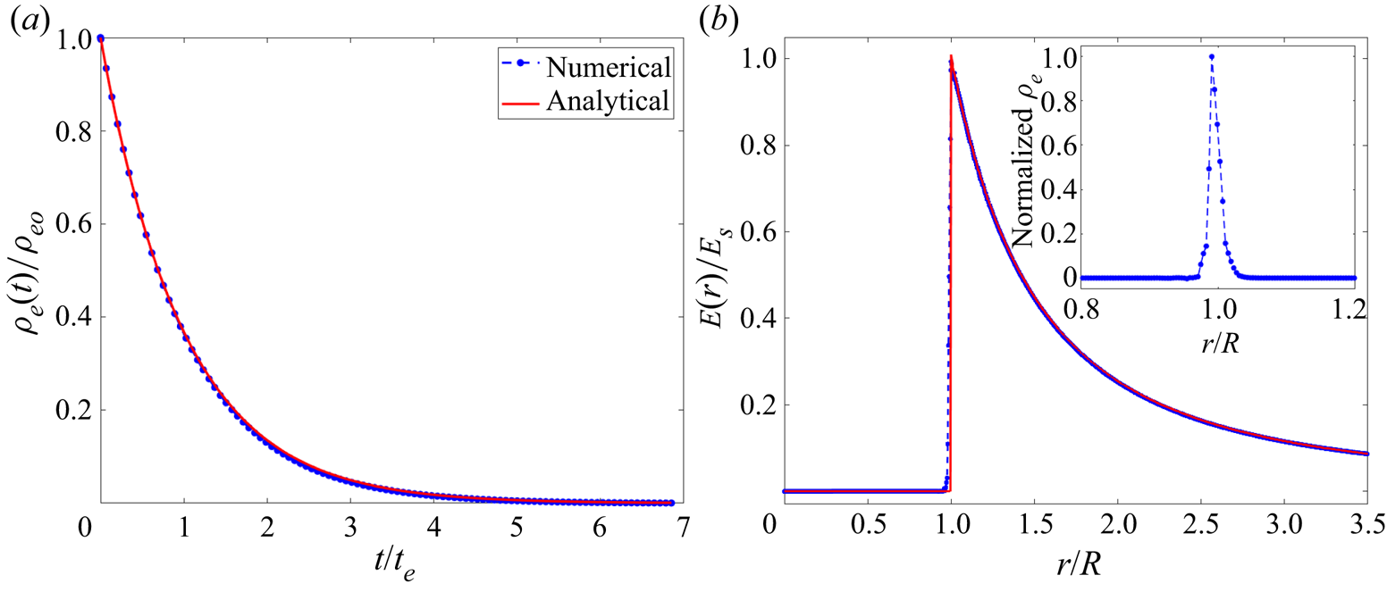
Figure 15. (a) Decay of the volumetric charge density inside the droplet (analytical and numerical solutions); (b) jump of the electric field across the surface of the droplet upon charge relaxation (analytical and numerical solutions). Inset shows the distribution of the volumetric charge.
Appendix C. Grid independence test and overall charge conservation
The numerical discretization should not cause significant charge loses. We next test several grid sizes to verify that charge is conserved in our simulations in the case of a droplet undergoing a Coulomb explosion (the total charge must be constant before the detachment of droplet progenies). We also analyse the sensitivity of the droplet and jet profiles to changes in the resolution of the grid. Among all conditions studied in this article, the smallest jet radii occur in droplets undergoing PRF; therefore, the tests in this appendix are worst-case scenario.
Figure 16 compares several figures of merit for four different grid resolutions in region A ( $h=$
$h=$  $R/128$, $R/96$, $R/64$, $R/42$ and $R/27$). The interface thickness parameter is always set such that $\xi =0.64h$. Figure 16(a) shows the evolution of the aspect ratio with time. Figure 16(b) demonstrates that the total charge is conserved well by any of the grid resolutions. Figure 16(c) compares the profile of the droplet for the different grid resolutions, while figure 16(d) shows the error $\epsilon$ in the position of the surface, $S(z)$, relative to the position computed with the grid of highest resolution, $h=R/128$:
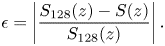 \begin{equation} \epsilon=\left|\frac{S_{128}(z)-S(z)}{S_{128}(z)}\right|. \end{equation}
The largest deviation occurs near the transition region of the jet. For  $h=R/64$, the maximum error is roughly $3\unicode{x2013}4\,\%$. For grid resolutions of $R/128$, $R/96$ and $R/64$, the aspect ratios and the surface profiles reasonably coincide, while the charge is well conserved. Therefore, to optimize the computational time, we have decided to use the $R/64$ grid in all calculations.

Figure 16. Grid independence test for a PRF droplet, using grid resolutions  $h=R/128, R/96, R/64, R/42, R/27$: (a) comparison of the aspect ratio versus time; (b) variation of the total charge with time; (c) profiles of the droplet once after formation of the jet; (d) error in the droplet profiles relative to that calculated with $h=R/128$, (C1).
It must be noted that one of the major caveats of using the phase field method in electrohydrodynamic problems is the use of an artificial diffuse interface of finite thickness. With regards to the modelling of jets, the resolution of radial features is limited by the thickness of the diffuse interface ( $R/100$ in our case). However, since this study focuses on ion emission from droplets and, as shown in figure 10, ion emission ceases once the jet is formed due to the lowering of the surface electric field, the limitations in the modelling of the jet do not affect the key findings.


 Open access