


1. Introduction
The goal of this study is to quantify the impact of turbulent fluctuations on the dynamics of coherent structures in the wake of a bluff body for both non-reacting and reacting conditions. Using this canonical configuration allows us to systematically vary the amplitude of coherent and turbulent oscillations in the flow field approaching the bluff body separately so that we can observe their interaction and their impact on flow response. This work is motivated by combustor operability issues like flame blowoff (Nair & Lieuwen Reference Nair and Lieuwen2007; Shanbhogue, Husain & Lieuwen Reference Shanbhogue, Husain and Lieuwen2009a; Chaudhuri et al. Reference Chaudhuri, Kostka, Tuttle, Renfro and Cetegen2011) and thermoacoustic combustion oscillations (Poinsot Reference Poinsot2017; O'Connor Reference O'Connor2022), where large-scale vortical structures arising from both hydrodynamic instability and thermoacoustic driving of the flow can dramatically impact the dynamics of the flame. However, it has been shown in bluff-body stabilized flames that the flame has a significant impact on the hydrodynamic oscillations in the flow field (Erickson & Soteriou Reference Erickson and Soteriou2011; Emerson et al. Reference Emerson, O'Connor, Juniper and Lieuwen2012), and so both non-reacting and reacting conditions are considered in this study to better understand these effects.
Coherent vortex shedding in the wake of bluff bodies is a complex phenomena that has received significant treatment in the literature (Williamson Reference Williamson1996b). The dynamics of the flow are strong functions of the Reynolds number, the level of backflow in the wake and the density of the wake relative to the free stream (Yu & Monkewitz Reference Yu and Monkewitz1990). In constant-density conditions, the wake of a cylindrical bluff body first displays oscillations at a Reynolds number of  $Re\approx 49$ (Jackson Reference Jackson1987; Williamson Reference Williamson1996b). For $Re>49$, this anti-symmetric vortex shedding mode is known as the von Kármán vortex street (Provansal, Mathis & Boyer Reference Provansal, Mathis and Boyer1987) and its oscillation frequency scales with the cylinder diameter (Prasad & Williamson Reference Prasad and Williamson1997). As the Reynolds number increases, the amplitude of the vorticity oscillations increases while the vortex formation length decreases and the peak vorticity fluctuation location moves upstream (Gerrard Reference Gerrard1966; Williamson Reference Williamson1996a). At higher values of Reynolds numbers ( $1000< Re<200\,000$), the Strouhal number of the primary vortex shedding mode is relatively independent of Reynolds number and has a constant value of $St_D \approx 0.21$, where $St_D=fD/U$ (Cantwell & Coles Reference Cantwell and Coles1983). This range of Reynolds number is also where the shear layers separating from the bluff body display oscillations, a manifestation of the Kelvin–Helmholtz instability (Bloor Reference Bloor1964; Prasad & Williamson Reference Prasad and Williamson1997).
Free-stream turbulence can impact vortex shedding in the wakes of bluff bodies. Several studies have shown that increasing free-stream turbulence intensity can decrease the vortex formation length, which limits the downstream development of the shear layer and promotes merging of the shear layers downstream of the bluff body (Bloor Reference Bloor1964; Gerrard Reference Gerrard1966; Arie et al. Reference Arie, Kiya, Suzuki, Hagino and Takahashi1981; Norberg Reference Norberg1986). Khabbouchi et al. (Reference Khabbouchi, Fellouah, Ferchichi and Guellouz2014) showed that, in addition to shortening the vortex formation length, increasing free-stream turbulence intensity accelerates the breakdown of vortices, thereby disrupting their coherence. They suggested that increasing turbulence intensity has qualitatively similar effects to increasing the bulk Reynolds number. Turbulent motions also have an effect on the evolution of coherent vortices in a shear flow. Turbulence can act to ‘decorrelate’ the motions of coherent vortices in two ways. First, turbulent diffusion can reduce the peak vorticity in a structure (Arie et al. Reference Arie, Kiya, Suzuki, Hagino and Takahashi1981; Khabbouchi et al. Reference Khabbouchi, Fellouah, Ferchichi and Guellouz2014). Additionally, turbulence can cause phase jitter, which causes cycle-to-cycle variations in the location of a coherent vortex, lowering phase-averaged vorticity (Shanbhogue, Seelhorst & Lieuwen Reference Shanbhogue, Seelhorst and Lieuwen2009b). In this study we do not attempt to discern between these two effects, like we have in previous work (Karmarkar et al. Reference Karmarkar, Frederick, Clees, Mason and O'Connor2019).
This study focuses on the response of turbulent wakes to harmonic excitation. The response of flows to harmonic excitation depends on the global stability of the flow. In globally stable flows with regions of convective instability, flows can respond strongly to external excitation, even in the presence of high levels of turbulence. In mixing layers, for instance, vortex shedding occurs at the external excitation frequency (Ho & Huerre Reference Ho and Huerre1984; Fiedler & Mensing Reference Fiedler and Mensing1985; Gaster, Kit & Wygnanski Reference Gaster, Kit and Wygnanski1985); other more complex phenomena like vortex merging (Ho & Huang Reference Ho and Huang1982) and the formation of streamwise structures (Lasheras, Cho & Maxworthy Reference Lasheras, Cho and Maxworthy1986) can also be present. Similarly, the separating shear layers in bluff-body flows can respond such that the vortex shedding frequency matches that of the excitation (Provansal et al. Reference Provansal, Mathis and Boyer1987). However, constant-density wake flows are often globally unstable and display their own self-excited dynamics, which can change the nature of flow response to external excitation. The response of globally unstable flows can take multiple forms depending on the frequency and amplitude of excitation. One potential response is entrainment, where the oscillations of the global mode align with those of the external excitation at high enough forcing amplitudes (Griffin & Hall Reference Griffin and Hall1991). In wakes, the symmetry of the imposed excitation can change the response of the global mode. While the primary mode of vortex shedding in the wake is the anti-symmetric von Kármán mode, the presence of symmetric excitation can compete with the natural anti-symmetric oscillation. Konstantinidis & Balabani (Reference Konstantinidis and Balabani2007) showed that harmonic longitudinal excitation can induce a symmetric vortex shedding pattern in the near-wake region of a cylindrical bluff body. Further downstream, the vortices become staggered and the dominant oscillation mode transitioned to an anti-symmetric mode. The number of cycles for which the symmetric vortices persisted in the near wake was dependent on the external excitation frequency and amplitude.
The presence of a density gradient can significantly alter the dynamics of wake flows. Local stability analysis by Yu & Monkewitz (Reference Yu and Monkewitz1990) showed that the nature of the mode, i.e. whether it is self-excited and whether the mode is symmetric or anti-symmetric, is dependent on the backflow ratio and density ratio. From this analysis, they showed low-density wakes are convectively unstable over a range of backflow ratios, but constant-density and high-density wakes transition from convectively to absolutely unstable at a high enough backflow ratio. Building on this analysis, Emerson et al. (Reference Emerson, O'Connor, Juniper and Lieuwen2012) showed that the growth rate of the global mode in low-density wakes is also a function of the degree of spatial co-location between the density gradient and the velocity gradient. This analysis was supported by experiments in a vitiated bluff-body stabilized flame where the density ratio of the wake was varied by modifying the upstream temperature, and the location of the flame was varied by modifying the flame speed of the mixture. Moving the density gradient into the free stream destabilized the wake, resulting in anti-symmetric vortex shedding (Emerson, Noble & Lieuwen Reference Emerson, Noble and Lieuwen2014). Similar results were found in simulations by Erickson & Soteriou (Reference Erickson and Soteriou2011).
Just as in non-reacting wakes, the presence of coherent excitation can have a significant impact on the dynamics of reacting wakes. Emerson & Lieuwen (Reference Emerson and Lieuwen2015) analysed the growth of the individual symmetric and anti-symmetric modes in a longitudinally excited reacting wake at a range of forcing frequencies. The longitudinal acoustic excitation promoted the growth of the symmetric mode in the near-wake region, which competed with the anti-symmetric vortex shedding modes in cases where the density ratio was sufficiently low for the global instability to manifest. Their results showed that when the forcing frequency approached the global mode frequency, resonant amplification caused the wake to respond strongly. In these cases, the vortices initially rolled up in a symmetric configuration but quickly staggered to an anti-symmetric pattern. At this resonant condition, the growth rate of the anti-symmetric mode was higher than that of the symmetric mode and nonlinear coupling between the anti-symmetric and symmetric modes was present at the first harmonic of the oscillation.
The results of this work can have significant implications for the dynamics of flames present in these oscillating flow fields, which are used in a variety of gas turbine combustor technologies (Lefebvre & Ballal Reference Lefebvre and Ballal2010). In these configurations, the flame is stabilized in the separating shear layer, which causes coupling between the flame and shear-layer fluctuations. Vortices present in the flow propagation along the flame stabilized in the separating shear layer of a bluff body, where the shed vortex causes perturbation in the flame area and, hence, heat release as it convects along the length of the flame (Renard et al. Reference Renard, Thevenin, Rolon and Candel2000; Chaparro, Landry & Cetegen Reference Chaparro, Landry and Cetegen2006). The flame response to a vortical disturbance can depend on the size and rotational strength of the vortex (Poinsot, Veynante & Candel Reference Poinsot, Veynante and Candel1991; Mueller et al. Reference Mueller, Driscoll, Reuss, Drake and Rosalik1998). Free-stream turbulence can also have a significant impact on the behaviour of flames. In particular, the propagation speed of a flame is directly modulated by free-stream turbulence (Driscoll Reference Driscoll2008; Chowdhury & Cetegen Reference Chowdhury and Cetegen2017). The modulation of flame speed by local flow oscillations is of particular significance in acoustically excited flames, as the burnout of large-scale flame wrinkles occurs faster at higher flame speeds (Roy & Sujith Reference Roy and Sujith2019). Shin & Lieuwen (Reference Shin and Lieuwen2013) showed, using a level-set approach, that the ensemble-averaged turbulent burning velocity is modulated by harmonic forcing with an inverse dependence upon ensemble-averaged flame curvature. In this way, the turbulent and coherent velocity fluctuations determine the speed at which the flame propagates, and, hence, the location at which the flame stabilizes in the flow field.
Our previous work (Karmarkar et al. Reference Karmarkar, Tyagi, Hemchandra and O'Connor2021) considered the impact that varying levels of turbulence intensity and bulk flow velocity had on the coherent vortex shedding in this same configuration in the absence of acoustic forcing. By varying these two parameters independently, we could observe the impact that the offset between the flame and the shear layer had on the coherent oscillations in the flow. The results showed that increasing the offset between the flame and the shear layer, either by reducing the mean-flow velocity or increasing turbulence intensity, enhanced anti-symmetric oscillations in the wake. However, increasing turbulence also increased the level of forcing in the system, resulting in stronger excitation of the anti-symmetric mode. In this way, higher turbulence intensity resulted in stronger anti-symmetric oscillations through two mechanisms: increasing flame/shear offset and noise forcing of the weakly stable anti-symmetric mode.
In the current work we build on this previous result by adding longitudinal acoustic forcing at a single bulk flow velocity, two turbulence intensities, and both non-reacting and reacting conditions. A single bulk velocity is chosen for two reasons. First, the velocity chosen allows for the largest operating range in terms of acoustic excitation without flame blowoff. Second, the previous study showed that the flow is much more sensitive to changes in turbulence intensity than bulk flow velocity. The non-reacting conditions are added to understand the interaction between coherent and turbulent oscillations of varying amplitudes in a constant-density system. These results provide an important baseline for understanding the reacting results, where the flame acts as a density gradient. Acoustic forcing is targeted at the wake shedding frequency with varying amplitudes to observe two effects: the nonlinear interaction between the wake instability and the external excitation, as well as the interaction between the anti-symmetric wake mode and the symmetric acoustic forcing. The results of this work identify the complex impact that turbulence has on flow dynamics in relevant combustor flows. In addition to modifying flame speed and driving weakly stable modes, as was found in the previous study, turbulence also modifies the behaviour of externally driven coherent oscillations. How these externally driven coherent oscillations interact with the oscillations arising from instability in the flow is the focus of this work. We find that the interaction between the two sources of coherent vortical motion in the flow, externally driven and global instability, is highly dependent on the turbulence intensity and the presence of the flame. Although this interaction has significant implications for flame dynamics, the focus of the current work is the flow behaviour; future work will address the flame response.
2. Methods
2.1. Experiment
The experimental facility is a modified version of that used by Tyagi et al. (Reference Tyagi, Boxx, Peluso and O'Connor2019) and so only a brief overview is provided here. The experiment is a rectangular burner that measures  $30\,{\rm mm} \times 100\,{\rm mm}$ at the burner exit with a 100 mm long, 3.18 mm diameter rod that runs along the centre of the burner, as shown in figure 1. The flame is stabilized on this cylindrical bluff body. A stoichiometric premixed mixture of air and fuel (natural gas) enter through the base of the burner and pass through two ceramic honeycomb flow straighteners. We use perforated plates in varying configurations for turbulence generation. The turbulence generation plates have a staggered hole pattern with 3.2 mm hole diameters and a 40 % open area. Two perforated plates located 10 and 30 mm upstream of the burner exit are used for the high inflow turbulence intensity (11 %) conditions and no perforated plates are used for low inflow turbulence intensity (5 %) conditions. The bulk flow velocity is held constant at 10 m s $^{-1}$ ( $Re_D=2036$) in all conditions presented. External acoustic excitation is added using a speaker at the base of the burner, upstream of both honeycombs, as shown in figure 1. The input to the speaker is an amplified sinusoidal signal generated by a waveform generator. The frequency of the input signal is set to 580 Hz, which is close to the characteristic frequency of vortex shedding and corresponds to a Strouhal number, $St_D=0.19$. The amplitude of acoustic excitation is varied by adjusting the peak-to-peak voltage ( $V_{pp}$) of the input signal.

Figure 1. Experimental facility.
2.2. Diagnostics
Stereoscopic particle image velocimetry is performed at a sampling rate of 10 kHz with a dual cavity, Nd:YAG laser (Quantronix Hawk Duo) operating at 532 nm in forward-forward scatter mode. A 50 mm tall laser sheet is created using a combination of mirrors and three cylindrical lenses; the angle between the laser sheet and each camera sensor (Photron FASTCAM SA5) is about  $35^{\circ }$. Each camera is equipped with a 100 mm f/2.8 lens (Tokina Macro) and a Nikon tele-converter to allow for a safe stand-off distance between the sensor and the burner. This set-up has a $32\,{\rm mm} \times 53\,{\rm mm}$ field of view and images are collected at 10 kHz in double-frame mode with a pulse separation of 14 $\mathrm {\mu }$s. Aluminum oxide particles of diameters 0.5–2.0 $\mathrm {\mu }$m are used for seeding. To reduce flame luminosity in the images, near-infrared filters (Schneider Kreuznach IR MTD) and laser line filters (Edmund Optics TECHSPEC 532 nm CWL) are used on each camera. LaVision's DaVis 8.3 is used to perform vector calculations from Mie-scattering images. These calculations include a multi-pass algorithm with varying window sizes ranging from $64 \times 64$ to $16 \times 16$ and a 50 % overlap. This processing results in a vector spacing of 0.48 mm vector $^{-1}$. A universal outlier detection scheme, with a 3 $\times$ median filter, is used for post-processing of the vector fields. The instantaneous uncertainties in the vector fields range from 1.5–2.8 m s $^{-1}$ in the reacting conditions and 0.7–2.1 m s $^{-1}$ in the non-reacting cases, using the uncertainty calculation feature in Davis. The uncertainties in the root-mean-square (r.m.s.) magnitude of the vector fields range from 0.03–0.05 m s $^{-1}$ in all cases. A total of 5000 vector fields are obtained for each condition.
The Mie-scattering images from PIV are also used to identify the flame location. The process for binarization and edge detection in the Mie-scattering images includes five steps. First, images are Gaussian filtered for blurring sharp gradients due to noise. Second, median filtering with a window size of 10 pixels  $\times$ 10 pixels is applied to remove the effect of salt and pepper noise due to scattering from the aluminum oxide particles. Next, a smoothing operation is performed using bilateral filtering, and then Otsu's method is applied on the smoothed image and multi-level thresholding is used to account for the spatial variation in signal intensity; the number of thresholds is varied between 4 and 8 depending on the conditions. Finally, the minimum threshold value is used to binarize the processed image into a value of 0 in the reactants and 1 in the products. These binarized images are used to calculate the time-averaged and phase-averaged progress variable contour, $\bar {c}$.
2.3. Data analysis
2.3.1. Triple decomposition
In statistically stationary flow fields, any flow variable,  $f(x,y,t)$, can be decomposed into three components: a time-averaged value, the coherent component and a turbulent component (Hussain Reference Hussain1983), i.e.
 \begin{equation} f(x,y,t)=\bar{f}(x,y)+\tilde{f}(x,y,t)+f''(x,y,t). \end{equation}
In this study, we perform the triple decomposition of a flow variable at a given spatial location,  $(x,y)$, using the following steps. First, we spatially average the quantity over a $3\times 3$ pixel window to avoid any spurious results from a single PIV interrogation window. We then compute the time-averaged component, $\bar {f}(x,y)$. A Fourier transform is then performed on the total fluctuating component, $f(x,y,t)-\bar {f}(x,y)$. The signal is then filtered in the frequency domain around the frequency of excitation (width of the filter, $\varDelta _f=40\,{\rm Hz}$) and then reconstructed to obtain the coherent component $\tilde {f}(x,y,t)$. Finally, the turbulent component, $f''(x,y,t)$, is computed by reconstructing the fluctuating velocity signal without the content at the forcing frequency and its first harmonic. The turbulence intensity is calculated by dividing the r.m.s. of the three components of fluctuating velocity by the bulk flow velocity and indicated by the symbol $u'$.
$u'$.
2.3.2. Instantaneous phase difference analysis
In this study, we use the Hilbert transform to analyse the symmetry of the shear layer and centreline oscillations. The Hilbert transform generates a complex time series, the magnitude of which provides the envelope of the original time series and the phase of the complex time series provides the instantaneous phase of the signal. The relative instantaneous phase can be compared between two simultaneous time series to quantify their phase difference. This method is especially useful in obtaining the phase difference between two intermittent oscillation signals or signals that are varying in frequency with time. Using the hilbert function in Matlab, we compare two time series across a plane of symmetry and compute the phase difference between the two signals as a function of time. We then compute a probability density function of the phase by fitting the phase data to the non-parametric empirical kernel distribution to quantify the variation in phase difference at every downstream condition. We use the values of the probability density function to estimate the likelihood of a anti-symmetric (in-phase) or symmetric (out-of-phase) oscillation. We use the non-parametric kernel distribution to avoid making any assumptions about the distribution of the phase differences.
2.3.3. Spectral proper orthogonal decomposition
The spectral proper orthogonal decomposition (SPOD) method by Towne, Schmidt & Colonius (Reference Towne, Schmidt and Colonius2018) is used to identify and characterize the dominant coherent oscillation modes in the flow. The SPOD method decomposes the data into an optimal orthogonal set of basis functions, or modes, which are sorted in decreasing order of modal energy, or variance, of the data. The SPOD method is advantageous as it captures oscillations that are coherent in space and time. The decomposition yields a set of eigenvalues at each frequency and spatial eigenvectors corresponding to each eigenvalue and frequency. This method allows us to visualize the oscillations in the flow field that exhibit high values of spatio-temporal coherence. In this study, we use SPOD to decompose the time-varying vorticity field. For each condition, we have  $5000$ samples obtained at a sampling rate of 10 kHz. The SPOD calculation uses $256$ snapshots per block with a $50\,\%$ overlap, which results in 38 total blocks. The frequency resolution of the resulting spectra is 40 Hz.
2.3.4. Wavelet transforms
Wavelet transforms are implemented to observe the frequency content of a time-varying velocity or vorticity signal at a given location in the flow. Wavelet transforms are advantageous because, unlike a Fourier transform, wavelet transforms allow for the characterization of inherently non-stationary signals, such as those seen in flows that experience intermittent coherent oscillations. In order to compute the wavelet transform, we first average the velocity or vorticity signal at a location in the flow over a  $3\times 3$ pixel window. We then subtract the time-averaged value from the signal and perform the wavelet transform on the fluctuating component. We use the cwt function in MATLAB to compute the wavelet transform and we use the Morse wavelet.
2.4. Test conditions
In this study, we analyse how coherent and turbulent fluctuations can impact the response of both non-reacting and reacting wake flows. To quantitatively characterize the magnitudes of turbulent and harmonic oscillations in the incoming flow, we collect data at free-stream conditions without the cylindrical bluff body in place. We do this because the flow field upstream of the cylindrical bluff body is not optically accessible and the free-stream measurements without the bluff body provide a reasonable estimation of the ‘input’ flow fluctuations. We perform a triple decomposition on the velocity field along the centreline at 0.8 mm downstream of the burner exit. Figure 2 shows the individual turbulent and harmonic components obtained from the triple decomposition at varying levels of acoustic excitation (quantified in volts supplied by the waveform generator,  $V_{pp}$) for both the high-turbulence (two turbulence-generating plates) and low-turbulence (zero plates) conditions.

Figure 2. Triple decomposition of the free-stream velocity measurements: (a) variation in turbulence intensity (r.m.s.) with plates and input excitation voltage, (b) variation in harmonic velocity oscillation amplitude (r.m.s.) with plates and input excitation voltage, and (c) variation in the ratio of coherent to turbulent oscillation amplitude with plates and input excitation voltage.
Figure 2(a) shows the variation in the turbulent component of the input fluctuation normalized by the mean-flow velocity as a function of acoustic excitation amplitude. Acoustic excitation does not significantly impact the turbulent fluctuation amplitude. Furthermore, the perforated plates add significantly to the turbulence intensity, where the turbulence intensity ( $u'_{in}/\bar {u}_{in}$) is around 5 % for the condition with no perforated plates and 11 % for the conditions with both plates in place. Figure 2(b) shows the coherent component ( $\tilde {u}_{in}/\bar {u}_{in}$), which varies linearly with excitation voltage, $V_{pp}$. Importantly, the presence of the perforated plates minimally impacts the coherent content. This characterization shows that using the perforated plates and the acoustic excitation from the speaker, we can control the magnitudes of the turbulent and coherent fluctuations separately. Finally, figure 2(c) shows the relative coherent-to-turbulent input fluctuations for both plate conditions. There are three conditions, marked by the black horizontal lines, where the ratios of coherent and turbulent fluctuations are comparable for the two turbulence intensities: the no-forcing case (0 %), 32 % and 55 %. These conditions will be used for comparing different levels of coherent and turbulent oscillation amplitudes.
3. Non-reacting flow results
3.1. Time-averaged flow fields
The time-averaged vorticity is shown in figure 3 for both turbulence intensities (rows) and at all levels of acoustic excitation (columns). The top edge of the cylindrical bluff body is located at the base of the flow field ( $x=0$ mm, $y=0$ mm). The black solid contour depicts the time-averaged recirculation zone boundary, represented by $\bar {u}_y=0$. The black dotted lines depict the time-averaged shear layers separating from the bluff body. To compute the shear-layer locations, we first identify the location of the peak time-averaged vorticity magnitude at every downstream distance and then perform a linear fit through the identified points. The plots in figure 3 show that for a given turbulence intensity, acoustic excitation does not significantly impact the time-averaged vorticity field. The turbulence intensity, however, changes the time-averaged structure of the flow field. The high-turbulence conditions have a smaller recirculation zone than the low-turbulence conditions at each level of acoustic forcing. Furthermore, the magnitude of the peak vorticity in the separating shear layers on either side of the bluff body is higher in the low-turbulence conditions. These results are consistent with findings in the literature (Gerrard Reference Gerrard1966; Khabbouchi et al. Reference Khabbouchi, Fellouah, Ferchichi and Guellouz2014). Figure 4 shows centreline profiles of the time-averaged streamwise velocity as a function of downstream distance for both the low- (a) and high-turbulence (b) conditions. The length of the recirculation zone, $L_{RZ}$, can be quantified as the distance from the trailing edge of the bluff body to the zero crossing of the centreline velocity field; the recirculation zone is shorter in the high-turbulence condition ( $L_{RZ}=2.5$ mm) than in the low-turbulence condition ( $L_{RZ}=5$ mm). In the low-turbulence condition only, increasing acoustic excitation amplitude increases the strength of recirculation, quantified by the minimum velocity along the centreline.

Figure 3. Time-averaged vorticity contours with the recirculation zone ( $\bar {u}_y=0$) shown in the solid black contour; the dotted black lines represent the time-averaged shear layers. Plots (a–f) correspond to the condition with no plates ( $TI=5\,\%$) and (g–l) correspond to the condition with both plates ( $TI=11\,\%$).

Figure 4. Time-averaged centreline velocity of the  $TI=5\,\%$ condition (a) and the $TI=11\,\%$ condition (b) for all levels of acoustic excitation.
Figure 5 shows the spatial distribution of the r.m.s. of the total fluctuating vorticity in the flow field. The plots in the top row correspond to the turbulence intensity of  $5\,\%$ and the plots in the bottom row correspond to the conditions with a higher free-stream turbulence intensity of $11\,\%$. In the high-turbulence conditions, higher fluctuation levels are present in the flow field at the base of the domain near the burner exit, a consequence of the higher turbulent velocity fluctuations generated by the perforated plates. In all conditions, a region of high fluctuation is located at the trailing end of the time-averaged recirculation zone. This vorticity fluctuation is a result of anti-symmetric vortex shedding from the bluff body, where the vortex formation length is the distance from the trailing edge of the bluff body to the location of peak r.m.s. (Williamson Reference Williamson1996b). In the low-turbulence conditions, the region with high vorticity fluctuation amplitude downstream of the recirculation zone increases in both size and strength as the acoustic excitation amplitude increases. In high-turbulence conditions, the region with high values of fluctuation amplitude is smaller and the peak magnitude is lower as compared with the conditions with low free-stream turbulence. Furthermore, the r.m.s. field is less altered by acoustic excitation in the high-turbulence case than the low-turbulence case.

Figure 5. The r.m.s. of the fluctuating vorticity field ( $\omega '$) with the recirculation zone depicted by the solid black contour ( $\bar {u}_y=0$), and the shear layers depicted by the dotted black lines, for all excitation amplitudes at both turbulence intensities.
To understand the vortex dynamics behind the bluff body, we use wavelet transforms of the vorticity signal at dynamically significant regions of the flow. A probe location is selected at the peak vorticity location in the shear layer and a time series is constructed from the average signal in a  $3\times 3$ interrogation-window region; the wavelet magnitude scalograms of that time series are calculated for each condition. The two boundary cases – no external excitation and the highest level of acoustic excitation – are shown in figure 6; the scalograms at all intermediate conditions are provided in the supplementary material available at https://doi.org/10.1017/jfm.2023.321. In the absence of acoustic excitation, coherent content at a Strouhal number of $St_D=0.19$ is present in the vorticity fluctuations (close to the theoretical predicted value of $St_D=0.21$ for wakes), although the signal is spectrally broad and intermittent in time. The high-turbulence condition has stronger coherent oscillations in the absence of external acoustic excitation with less intermittency than the low-turbulence conditions. This behaviour is evidence of noise forcing of the oscillations in the wake. If the flow was strongly globally unstable, a relatively continuous oscillation at $St_{D}=0.19$ would be expected with some spectral broadening due to turbulence. However, the backflow ratio of this isothermal wake is relatively low, which likely means that it is marginally stable. These scalograms indicate that the system is near a stability boundary, as increasing the level of noise in the system produces more coherent oscillatory behaviour at the natural shedding frequency. In the conditions with maximum acoustic excitation, the low-turbulence condition exhibits a strong, continuous response at the forcing frequency, whereas the response in the high-turbulence condition is lower and has a greater degree of intermittency.

Figure 6. Wavelet magnitude scalograms at conditions with no external excitation (a,c) and the maximum acoustic excitation (b,d) for both turbulence intensities. Scalograms for all intermediate conditions are provided in the supplementary material.
3.2. Downstream development of coherent vorticity
In order to isolate the effects of the acoustic and turbulent excitation on the coherent vorticity dynamics, we now consider the evolution of coherent vorticity, calculated using the triple decomposition, along the shear layers and centreline. Figure 7 shows the evolution of the coherent vorticity component,  $\tilde {\omega }$, computed along the shear layer (a,c) and along the centreline (b,d) at both turbulence conditions. The colours from blue to red indicate increasing acoustic excitation amplitude. In both turbulence conditions, increasing excitation leads to an increasing response along the shear layer. In the low-turbulence conditions (a,b) the response peaks at around $y=2.69$ mm and decays to a negligibly small amplitude for $y>20$ mm. The high-turbulence conditions show a similar trend with acoustic excitation amplitude, but the magnitude of coherent vorticity fluctuation is much lower than at the low-turbulence condition. The right column in figure 7 shows the coherent vorticity along the centreline at all excitation amplitudes for both turbulence intensities. In the low-turbulence condition the amplitude of the peak response initially increases and then decreases with increasing amplitude. At maximum excitation, the location of the peak response shifts slightly downstream. In the high-turbulence conditions, shown in the bottom row, the coherent response along the centreline is actually stronger than that of the low-turbulence condition, opposite of the trend in shear-layer response.

Figure 7. Coherent vorticity amplitude along the shear layer (a,c) and along the centreline (b,d) with downstream distance for both turbulence intensities. Colours from blue to red indicate increasing levels of acoustic excitation.
The trends in coherent vortical response with acoustic excitation in the shear layers and the centreline can be understood by considering how the mode of vortex shedding changes with increasing acoustic excitation amplitude. In this wake, where  $Re_D\approx 2000$, the primary instability mode is the von Kármán vortex shedding mode, which is characterized by an anti-symmetric vortex shedding along the centreline of the flow field (Williamson Reference Williamson1996b). In both the low- and high-turbulence conditions in the absence of acoustic forcing, the coherent oscillation along the centreline is greater than that in the shear layers because this anti-symmetric vortex shedding mode dominates. However, introducing longitudinal acoustic excitation drives symmetric vortex shedding in the shear layers separating from the bluff body, which is why the magnitude of coherent fluctuation in the shear layers increases with increasing acoustic amplitude. The differences in the response of the low-turbulence versus high-turbulence cases can be explained by considering the response of a noise-forced oscillator. While the longitudinal acoustic forcing drives the symmetric shear-layer response, the centreline anti-symmetric vortex shedding is excited by the turbulent fluctuations. Even in the presence of high-amplitude symmetric acoustic forcing, the centreline coherent response (indicative of anti-symmetric oscillations) is higher in the high-turbulence case than the low-turbulence case.
The opposite trend is found in the shear layers, as turbulence tends to decorrelate the acoustically excited motions in the shear layers and turbulence intensity is particularly high in the shear layers due to both the incoming and shear-generated turbulence. In the high-turbulence conditions, the integral length scale is of the order of  $\sim$2 mm. At the peak vorticity location, the turbulent intensity $u'/U=17\,\%\unicode{x2013}20\,\%$, indicating that the shear-generated turbulence is stronger than the free-stream turbulence. The magnitude of shear-generated turbulence in the peak vorticity location is comparable for both the low and high inflow turbulence intensity conditions. As such, differences in the flow at the two different inflow turbulence intensities are, in part, driven by the variation in inflow turbulence intensity rather than any differences in shear-generated turbulence. To better understand the mechanisms that contribute to the weakening of the coherent response in the shear layers, we look at the variation in coherent vorticity for both inflow turbulence conditions at comparable relative coherent-to-turbulent forcing conditions (constant $\tilde {u}_{in}/u'_{in}$) in figure 8. For the same $\tilde {u}_{in}/u'_{in}$, the coherent shear-layer response in the high-turbulence conditions is weaker than in the low-turbulence conditions. This difference is due to the fact that the primary instability mode of oscillation is different in the low- and high-turbulence conditions and the presence of a strong anti-symmetric mode in the high-turbulence conditions reduces the response of the shear layers to acoustic excitation.

Figure 8. Comparing coherent vorticity along the shear layer for comparable relative coherent-to-turbulent input forcing conditions.
To better quantify the interaction between turbulence-driven anti-symmetric oscillations and acoustically driven symmetric oscillations, we compute the instantaneous phase difference between the oscillations along the shear layers and on either side of the centreline. To quantify the symmetry of the coherent fluctuations, we calculate a statistical distribution of the phase difference,  ${\rm \Delta} \varPhi$, of vorticity fluctuations between shear layers on either side of the centreline at every downstream location. The probability of anti-symmetric (in-phase) motion is defined as $P(345^{\circ }<{\rm \Delta} \varPhi <15^{\circ })$, whereas the probability of symmetric (out-of-phase) motion is defined as $P(165^{\circ }<{\rm \Delta} \varPhi <195^{\circ })$. This statistical methodology is used to capture not only the symmetry of the oscillations, but also to account for the inherent intermittency of these oscillations. The wavelet transforms in figure 6 capture both symmetric and anti-symmetric motion and show the high levels of intermittency in the signal, particularly in the low turbulence intensity cases. This statistical analysis captures both the symmetry and intermittency of the oscillations.
Figure 9 shows the likelihood of anti-symmetric and symmetric motion in the shear layers (a,c) and across the centreline (b,d) for both turbulence intensities at all excitation amplitudes. Overall, the likelihood of any given motion varies between a probability of 0.05 and 0.3, showing the high level of intermittency in the oscillations. In the low-turbulence condition and in the absence of excitation, the shear-layer response is more likely to be anti-symmetric, a result of driving by the Bénard-von Kármán instability in the wake. As the excitation amplitude increases, the shear-layer response in the upstream region is more likely to be symmetric. However, further downstream, the response is more likely to be anti-symmetric, similar to the findings reported by Konstantinidis & Balabani (Reference Konstantinidis and Balabani2007). For the same low-turbulence condition, the centreline oscillations are always more likely to be anti-symmetric, indicating that the von Kármán vortex shedding mode generally dominates the centreline oscillations, except in the near-wake region, where the probabilities of anti-symmetric and symmetric motion are very similar. With increasing excitation, the probability of symmetric motion increases, even along the centreline, indicating that the strong symmetric shear-layer response in these conditions is beginning to impact the anti-symmetric vortex shedding along the centreline. In the high-turbulence conditions, shown in the bottom row, the anti-symmetric vortex shedding mode is more likely in the shear layers at all forcing amplitudes. With increasing forcing, the probability of symmetric oscillation does increase, but the anti-symmetric mode always has the higher likelihood. In the high-turbulence condition the dominant oscillation mode across the centreline is always anti-symmetric, even in the near-wake region.

Figure 9. Probability of in-phase (anti-symmetric, AS) motion,  $P(345^{\circ }<{\rm \Delta} \varPhi <15^{\circ })$, depicted by solid lines and out-of-phase (symmetric, S) motion, $P(165^{\circ }<{\rm \Delta} \varPhi <195^{\circ })$, depicted by dotted lines, for both turbulence intensities at every downstream location for the shear layers (a,c) and the centreline (b,d). Colours from blue to red indicate increasing levels of acoustic excitation.
3.3. Analysis of dominant coherent oscillation modes using SPOD
The results in figure 9 provide statistical information about how free-stream turbulence determines the most likely coherent oscillation modes in the flow. To quantitatively capture the amplitudes of these modes and visualize their spatial structure, we perform a SPOD on the vorticity field at each condition. Figure 10 shows the eigenvalue spectra and spatial mode shapes at the peak frequencies for the conditions with no acoustic forcing (a,c) and the condition with maximum acoustic excitation (b,d) at both turbulence intensities. The spectra at all intermediate conditions are provided in the supplementary material. In the absence of acoustic excitation, for both turbulence intensities, the first mode exhibits a singular peak at the natural frequency of vortex shedding. Note the spectral broadness of the peaks; the peak in the low-turbulence case is much broader than that of the high-turbulence case, which is consistent with the trends shown in the wavelet spectrograms in figure 6. For both turbulence intensities in the absence of acoustic excitation, the dominant coherent oscillation is an anti-symmetric vortex shedding mode; the first mode captures all the coherent content.

Figure 10. Eigenvalue spectra and mode shapes corresponding to the peak frequencies for the first two vorticity modes, for conditions with no external excitation (a,c) and maximum acoustic excitation (b,d) for both turbulence intensities. Spectra and mode shapes for all intermediate excitation amplitudes are provided in the supplementary material.
At the maximum excitation amplitude (b,d), the modal spectra look significantly different. Importantly, spectrally narrowband features are evident in the first and second modes of the SPOD spectra for both the low- and high-turbulence conditions. The mode shape corresponding to the peak frequency in mode 1 ( $\lambda _1$) and mode 2 ( $\lambda _2$) are shown in the images to the right of the spectra. In the low-turbulence condition, mode 1 exhibits a symmetric oscillation pattern, shown in the top right figure. The spatial mode shape corresponding to the peak frequency in the second mode resembles an anti-symmetric vortex shedding mode, though some interference from the symmetric mode shape is present as well. By contrast, even at the highest excitation amplitude, the spatial mode shape corresponding to the peak frequency of the dominant mode ( $\lambda _1$) is anti-symmetric in the high-turbulence case; the peak of the second mode ( $\lambda _2$) shows a symmetric vortex shedding pattern. This mode is excited by the external excitation, but is still weaker than the natural vortex shedding mode in the high-turbulence condition. The separation of the modes in the high-amplitude forcing cases into generally symmetric and anti-symmetric motions is a result of their relative energies, not their symmetries. SPOD is not inherently able to recognize symmetry of a flow and attempts to first decompose the flow by symmetry before applying SPOD, as suggested by Schmidt & Colonius (Reference Schmidt and Colonius2020), were not successful. What the difference in mode shapes between mode 1 and mode 2 indicates is the relative energy associated with anti-symmetric and symmetric motions at different turbulence intensities, and this analysis method works relatively well because these motions have significantly different oscillation energies (almost an order of magnitude).
For a more quantitative comparison, we extract the mode amplitudes at the peak frequencies for the first two modes for all excitation amplitudes at both turbulence intensities. Figure 11 shows the energy of the first two modes at the peak frequency as a function of the acoustic forcing amplitude. In the conditions with low turbulence intensity (shown in blue), the dominant oscillation mode switches from anti-symmetric to symmetric at a critical excitation amplitude of  $\tilde {u}_{in}/\bar {u}_{in}=3\,\%$. This result illustrates the competition between the natural anti-symmetric vortex shedding mode and the symmetric mode forced by the acoustic excitation. In the high-turbulence conditions (shown in yellow), the dominant oscillation mode is always anti-symmetric and the second mode is always symmetric over the range of forcing amplitudes achievable in this experiment. However, the energy of the anti-symmetric mode does decrease with increasing excitation amplitude, a result of interference from the weaker symmetric oscillation mode. Put together, the results from the non-reacting wake show that increasing turbulence intensity can affect the response in two ways. First, increasing turbulence intensity can strengthen the natural anti-symmetric vortex shedding response along the centreline, likely a result of noise forcing of the weak global instability present in this flow. Second, increasing turbulence can weaken the symmetric response of the shear layers to the longitudinal acoustic excitation, likely the result of both interference with the stronger anti-symmetric mode and the decorrelating influence of turbulence on coherent structures.

Figure 11. Mode amplitudes and symmetry corresponding to the peak frequency for the first (solid lines) and second (dotted lines) SPOD modes at both turbulence intensities. The triangle and circle markers indicate the anti-symmetric (AS) and symmetric (S) mode shapes, respectively.
4. Reacting flow results
4.1. Time-averaged flow fields
The time-averaged vorticity in the reacting cases is shown in figure 12 for both turbulence intensities at all levels of acoustic excitation. The images show the shear-layer locations (dotted lines) as well as the most probable flame location (blue line), which is obtained by computing the time-averaged progress variable contour,  $\bar {c}=0.5$. Compared with the non-reacting conditions, the recirculation zones in the reacting conditions are larger, due to the expansion of gases across the flame. The plots in figure 13 show the variation of the time-averaged centreline streamwise velocity with downstream distance for all excitation amplitudes. In the low-turbulence condition (figure 13a), the recirculation zone becomes stronger and shorter with increasing excitation amplitude. The conditions with high turbulence intensity (figure 13b) are not significantly impacted by the acoustic excitation. These trends in flow structure mimic those of the non-reacting cases, but the variations in the reacting cases are amplified when compared with the non-reacting cases with the same turbulence intensity. This effect is due to the fact that the density of the wake has been substantially lowered by the addition of a flame. The flame stabilization location changes significantly with turbulence intensity and only slightly with acoustic forcing amplitude. In the high-turbulence conditions, the flame stabilizes at a wider angle than in the low-turbulence condition, which is due to the increase in turbulent flame speed. The flame stabilization angle slightly increases with increasing acoustic excitation amplitude in both the low- and high-turbulence conditions, which is a result of turbulent flame speed enhancement from the flame wrinkling due to acoustic excitation.

Figure 12. Time-averaged vorticity contours with the recirculation zone ( $\bar {u}_y=0$) shown in the solid black line contour; the dotted black lines represent the time-averaged shear layers and the solid blue lines depict the mean flame location ( $\bar {c}=0.5$).

Figure 13. Time-averaged centreline velocity of the  $TI=5\,\%$ condition (a) and the $TI=11\,\%$ condition (b) for all levels of acoustic excitation.
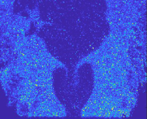
Figure 14 shows the r.m.s. of the fluctuating vorticity for both turbulence intensities at all excitation amplitudes. The fluctuation amplitudes for the reacting conditions look dramatically different to those for the non-reacting conditions shown in figure 5. In the low-turbulence conditions (figure 14a–f), regions of high fluctuation amplitude develop symmetrically along the shear layers on either side of the recirculation zone with increasing acoustic amplitude, suggesting a strong symmetric response in the vorticity dynamics along the shear layer at these conditions. At the high-turbulence conditions (figure 14g–l) and in the absence of external excitation, a region of high fluctuation is present downstream of the bluff body along the centreline, similar to the non-reacting conditions, suggesting some anti-symmetric vortex shedding may be present even in the reacting, low-density wake. This result was discussed in more detail in previous work (Karmarkar et al. Reference Karmarkar, Tyagi, Hemchandra and O'Connor2021). As the excitation amplitude increases, the fluctuations along the centreline are amplified and regions of high fluctuation develop along the shear layers as well.

Figure 14. The r.m.s. of the fluctuating vorticity field ( $\omega '$) with the recirculation zone depicted by the solid black contour ( $\bar {u}_y=0$), the shear layers depicted by the dotted black lines and the mean flame edge ( $\bar {c}=0.5$) depicted by the solid blue lines for all excitation amplitudes at both turbulence intensities.
Figure 15 shows the wavelet magnitude scalograms computed using the fluctuating vorticity signal at the peak vorticity location in the shear layers for both turbulence intensities at conditions with no external excitation and the condition with maximum acoustic forcing; scalograms for intermediate conditions are provided in the supplementary material. The horizontal black lines indicate the region of coherent von Kármán vortex shedding from the non-reacting conditions. In the absence of acoustic excitation (figure 15a,c), there is no coherent content at any frequency in the low-turbulence condition. This result suggests that this flow condition is globally stable and the low level of inlet turbulence does not excite any oscillations, as would be expected from a low-density wake with small flame/shear layer offset (Yu & Monkewitz Reference Yu and Monkewitz1990; Emerson et al. Reference Emerson, O'Connor, Juniper and Lieuwen2012). However, in the high-turbulence condition, highly intermittent coherent content is present at a range of frequencies. Previous work at this operating condition has shown that the wake behaves like a noise-forced oscillator and a weak, intermittent anti-symmetric oscillation mode is present even in the absence of excitation (Karmarkar et al. Reference Karmarkar, Tyagi, Hemchandra and O'Connor2021). The wake in the high-turbulence, reacting condition displays more oscillatory behaviour both because of the increased level of noise forcing and because of the increased offset between the shear layer and the flame, which destabilizes low-density wakes (Erickson & Soteriou Reference Erickson and Soteriou2011; Emerson et al. Reference Emerson, Noble and Lieuwen2014). At maximum values of acoustic excitation (figure 15b,d), flows at both inlet turbulence levels display a continuous and strong coherent response at the forcing frequency. When compared with the non-reacting conditions shown in figure 6, the response of the reacting wake to acoustic excitation is stronger for both turbulence intensities. The lower level of intermittency in the response is at least partially due to the enhanced viscous dissipation of turbulent fluctuations in the low-density reacting wake, which reduces the decorrelating motions of turbulence that were observed in the non-reacting cases. Additionally, the anti-symmetric mode is very weak in both cases, reducing the level of interaction between the acoustically excited symmetric motions and natural anti-symmetric motions.

Figure 15. Wavelet magnitude scalograms at conditions with no external excitation (a,c) and the maximum acoustic excitation (b,d) for both turbulence intensities. Scalograms at all intermediate conditions are provided in the supplementary material.
4.2. Downstream development of coherent vorticity
The r.m.s. fields of the fluctuating vorticity component show that the spatial structure of the fluctuating response in the reacting wake is strongly impacted by both the coherent excitation amplitude and the turbulence intensity. Figure 16 shows the variation in coherent vorticity along the shear layer (a,d), along the centreline (b,e) and along the flame stabilization location  $\bar {c}=0.5$ (c, f) for the conditions with low turbulence intensity (a–c) and the conditions with high turbulence intensity (d–f). We first consider the response of the shear layers. In the low-turbulence conditions (top), the strength of the vorticity response increases dramatically with increasing excitation amplitude. Unlike the non-reacting conditions, the amplitude of vorticity fluctuation does not decay monotonically with downstream distance past the peak; a local minimum in the response is observed for moderate acoustic excitation amplitudes at around $y=14$ mm, which is immediately downstream of the time-averaged recirculation zone. At the high-turbulence conditions, the coherent response along the shear layers is weaker than in the low-turbulence conditions, as was also seen in the non-reacting cases. Again, response amplitude increases with increasing acoustic excitation amplitude and the trend in vorticity fluctuation amplitude with downstream distance is non-monotonic after the initial peak. At almost all acoustic forcing conditions, a local minimum in response is located at around $y=9.5$ mm, which is immediately downstream of the time-averaged recirculation zone, and a second peak in the shear-layer response is present at $y=13.2$ mm. This oscillation in the amplitude of coherent vorticity is much more pronounced in the high-turbulence conditions. Figure 16(b,e) shows the downstream evolution of coherent vorticity along the centreline. For both turbulence intensities, the amplitude of the coherent response in the reacting conditions is significantly lower along the centreline than the shear layer. As in the non-reacting case, the coherent response along the centreline is higher for the high-turbulence condition than in the low-turbulence condition. For both turbulence intensities, the coherent vorticity along the flame location, shown in the right column, resembles the coherent vorticity decay along the shear layer. The oscillating decay pattern in the coherent vorticity along the shear layers is less pronounced along the flame location. This difference is primarily due to the increasing spatial offset between the flame and the shear layer with downstream distance. Further downstream, the coherent vortical disturbances along the flames are not as closely coupled with the vortical fluctuations along the shear layer.

Figure 16. Coherent vorticity variation along the shear layer (a,d), centreline (a,e) and the flame stabilization location  $\bar {c}=0.5$ (c, f) with downstream distance for both turbulence intensities. Colours from blue to red indicate increasing levels of acoustic excitation.
Figure 17 shows the coherent shear-layer vorticity for comparable relative coherent-to-turbulent input conditions at constant  $\tilde {u}_{in}/u'_{in}$. Unlike in the non-reacting cases, the amplitudes of the coherent response along the shear are comparable for both turbulence intensities at a given $\tilde {u}_{in}/u'_{in}$. The locations of peak vorticity fluctuation is further downstream in the low-turbulence condition as a result of the shortening of the recirculation zone with increasing turbulence intensity. Additionally, the interference pattern is more prominent in the high-turbulence case. This result illustrates that in the reacting conditions where a strong centreline oscillation mode is not present, the weakening of the shear-layer response with increasing turbulence intensity is not occurring. This difference is a result of differences in the interaction between the symmetric and anti-symmetric modes, as will be shown next.

Figure 17. Comparing the coherent vorticity with downstream distance for comparable relative input amplitudes for both turbulence conditions.
To understand the symmetry of the oscillation mode, we use the Hilbert transform to compute the instantaneous phase difference across the shear layers, the centreline and the two flame edges. The plots in figure 18 show the probabilities of anti-symmetric (solid lines) and symmetric (dotted lines) oscillations in the vorticity field at every downstream location in these three regions. Along the shear layer (figure 18a,d), the likelihood of symmetric oscillation looks very similar to the coherent vorticity distribution along the shear layer shown in figure 16. In the low-turbulence condition (figure 18a–c), the symmetric mode is always dominant, especially as the acoustic excitation is increased. With increasing downstream distance, the likelihood of symmetric oscillation decreases, but the symmetric mode still dominates. At the high-turbulence conditions (figure 18d–f), the symmetric mode dominates, but the probability along the downstream locations exhibits an oscillating decay pattern in both the anti-symmetric and symmetric components. Across the centreline (figure 18b,e), the oscillation is predominantly symmetric in the near field of the low-turbulence condition at high levels of excitation. However, further downstream, the dominant centreline oscillation mode is anti-symmetric. Increasing excitation amplitudes increase the likelihood of symmetric oscillation. The oscillations in the high-turbulence case are predominantly anti-symmetric along the centreline, even at high excitation amplitudes. Just like the phase difference across the shear layers, there is an oscillating decay pattern in both the anti-symmetric and symmetric components with downstream distance. However, the spatial wavelength in this interference pattern is greater along the centreline than in the shear layer. Finally, the third column shows the probabilities of anti-symmetric and symmetric oscillations in the vorticity field along the flame edge. The trends are largely similar to those in the shear layer without the presence of the interference pattern, owing to the distance between the flame and shear layer, particularly in the high-turbulence case.

Figure 18. Probability of in-phase (anti-symmetric, AS) motion,  $P(345^{\circ }<{\rm \Delta} \varPhi <15^{\circ })$, depicted by solid lines and out-of-phase (symmetric, S) motion, $P(165^{\circ }<{\rm \Delta} \varPhi <195^{\circ })$, depicted by dotted lines, for both turbulence intensities at every downstream location. Data obtained along the shear layers (a,d), centreline (b,e) and $\bar {c}=0.5$ contour (c, f). Colours from blue to red indicate increasing levels of acoustic excitation.
The results of the symmetry analysis suggest significant interaction between the symmetric and anti-symmetric modes in the wake, particularly in the high-turbulence conditions. Referring back to the trend in coherent vorticity fluctuation with downstream distance in figure 16 for the high-turbulence condition, the peaks and valleys of the coherent shear-layer response suggest an interference between the symmetric response of the shear layers and anti-symmetric behaviour in the wake. The interference between these two oscillations with the same frequency but different symmetries causes significant variations in the vortical oscillations with downstream distance. This reasoning is supported by the conceptual model described in the Appendix, where the two modes are modelled as travelling harmonic disturbances with a decay function to account for vortex formation and decay with downstream distance. Using representative values of oscillation frequency, phase and amplitude that closely match that from the experimental data, we show that this interference pattern seen in the vortical oscillation is driven by interaction between the anti-symmetric centreline mode and the symmetric shear-layer response.
4.3. Analysis of dominant coherent oscillation modes using SPOD
In order to characterize the amplitude of the individual modes and the symmetry of the dominant oscillations, we apply the SPOD method to the vorticity field of the reacting wake. Figure 19 shows the eigenvalue spectra and mode shapes corresponding to peak frequencies for the condition with no acoustic excitation (a,c) and the condition with maximum acoustic excitation (b,d) for the low turbulence intensity (a,b) and the high turbulence intensity (c,d) conditions. In the absence of acoustic excitation, no significant coherent content is present in the SPOD spectra for either turbulence intensity, indicating that the reacting wake is globally stable. At the maximum acoustic excitation amplitude, the low-turbulence condition exhibits a strong coherent response, which is almost entirely captured by the first mode. The mode shape of the first corresponding to the peak frequency, shown to the right of the spectra, is symmetric. The small peak at the second mode also exhibits a symmetric mode shape. At the high-turbulence conditions, the peak coherent response in mode 1 is lower than in the low-turbulence case but is still symmetric, as evidenced by the symmetric mode shape corresponding to the peak frequency of the first mode shown on the right of the spectrum. However, mode 2 contains a peak at the forcing frequency with a mode shape corresponding to an anti-symmetric vortex shedding pattern along the centreline. This result indicates that the increasing turbulence intensity excites the natural anti-symmetric vortex shedding mode, which is weaker than the symmetric vortex shedding mode but still spatially coherent.

Figure 19. Eigenvalue spectra and mode shapes corresponding to the peak frequencies for the first two modes for conditions with no external excitation (a,c) and maximum acoustic excitation (b,d) for both turbulence intensities. Spectra and mode shapes for all intermediate excitation amplitudes are provided in the supplementary material.
Like in the non-reacting conditions, we again extract the mode amplitude for the two leading modes at the peak frequency at every condition for both turbulence intensities and compare their strengths, which are shown in figure 20. For the low-turbulence conditions, both the modes are always symmetric at the peak frequency because the coherent response is dominated by the response to the external acoustic excitation. The mode amplitudes of the leading mode are also higher for the low-turbulence condition than the high-turbulence condition. In the high-turbulence condition, two different oscillation symmetries are present. The leading mode always exhibits a symmetric oscillation and the second mode is always an anti-symmetric mode shape. This result shows that increasing the free-stream turbulence intensity causes the anti-symmetric wake vortex shedding mode to be present even in the presence of high amplitudes of longitudinal excitation. As in the non-reacting wakes, the results show that turbulence has two direct impacts on the flow field response. First, high levels of turbulent fluctuations excite the natural anti-symmetric vortex shedding mode. Second, the turbulent fluctuations weaken the symmetric response of the shear layers to the longitudinal acoustic excitation through both interaction with the centreline anti-symmetric mode and through decorrelation of the coherent oscillations. The strong interference pattern of the vortical oscillations in the high-turbulence conditions in both the shear layers and centreline are evidence of the interaction between these two modes, resulting in lower response of the shear layer to external excitation.

Figure 20. Mode amplitudes and symmetry of the spatial mode shape corresponding to the peak frequency for the first (solid lines) and second (dotted lines) modes at both turbulence intensities. The triangle and circle markers depict the anti-symmetric (AS) and symmetric (S) modes, respectively.
5. Conclusions
This study presents an analysis of the impact of turbulence on the response of reacting and non-reacting wakes to external longitudinal acoustic excitation. The individual amplitudes of coherent and turbulent fluctuations can impact not only the amplitude but also the symmetry of the coherent flow response. In the non-reacting conditions in the absence of acoustic excitation, anti-symmetric vortex shedding is present. As the coherent excitation amplitude increases, the wake in the low-turbulence conditions exhibit a predominantly symmetric oscillation, although a weaker anti-symmetric oscillation mode is still present. In the high-turbulence conditions, the dominant oscillation mode is anti-symmetric, even at peak excitation amplitudes. A weaker symmetric mode is present at the peak excitation amplitude, but the dominant mode is always anti-symmetric. The dynamics of the reacting wakes are quite different from the non-reacting wakes. In the absence of external excitation, the reacting wakes are globally stable but increasing turbulence intensity and larger offsets between the shear layer and flame location can introduce spectrally broad, intermittent coherent oscillations (Karmarkar et al. Reference Karmarkar, Tyagi, Hemchandra and O'Connor2021). Even though the turbulence intensity in the shear layer is comparable for both the low and high inflow turbulence conditions, increasing the inflow turbulence intensity increases the spatial offset between the flame and the shear layer, which ultimately impacts the response of the flame to external excitation. As the coherent excitation amplitude increases, the flow in the low-turbulence conditions exhibits a strong symmetric response. The symmetric shear-layer response in the high-turbulence conditions is significantly lower and some anti-symmetric motion is present along the centreline. A clear interference pattern in the coherent vortical oscillation occurs as a result of interaction between the symmetric mode generated in response to the acoustic excitation and the anti-symmetric wake oscillation mode. We support this conclusion using a conceptual model, described in the Appendix. Even though the non-reacting conditions also experience the presence of competing modes of oscillation, an interference pattern is not visible in the shear-layer response. This effect is primarily due to the fact that the decay of coherent vorticity in the shear layers occurs more rapidly in the non-reacting conditions. In the reacting conditions, there is a significant decrease in turbulence intensity downstream of the flame as a result of the higher viscosity in the high-temperature products (O'Brien et al. Reference O'Brien, Towery, Hamlington, Ihme, Poludnenko and Urzay2017). The lower turbulence intensity results in less decorrelation of the coherent vorticity fluctuations in the reacting case.
Put together, the results of this study and our previous work on the unforced dynamics (Karmarkar et al. Reference Karmarkar, Tyagi, Hemchandra and O'Connor2021) show the multiple pathways by which turbulence can impact the coherent vorticity dynamics of reacting systems both with global modes. Figure 21 summarizes this interaction by identifying the connections between two types of coherent flow fluctuations (acoustically excited and the global mode), turbulent flow fluctuations and the flame. In this conceptual model, turbulent fluctuations affect each of the other actors in the flow field through modification of the flame speed and, hence, flame location, through turbulent dissipation and jitter, and through noise forcing of the global mode. The global mode is also significantly impacted by the presence of the flame and, in particular, the offset distance between the flame and the shear layer. The resultant interference between the acoustically excited fluctuations and the global mode determines the amplitude and symmetry of the coherent oscillations in the flow, which in turn can drive oscillations in the flame, notated here as combustion dynamics. The amplitude of the thermoacoustic coupling that can result from the driving of a flame by coherent velocity oscillations is not only dependent on the amplitude of the velocity oscillations, but also their symmetry (O'Connor Reference O'Connor2022). For example, anti-symmetric flame oscillations cannot drive symmetric acoustic fields, and so even though there may be significant flame oscillation, no thermoacoustic feedback is possible. While the response of the flame is not the focus of this study, this work provides an important foundation for understanding the development of velocity-coupled combustion dynamics in combustor flow fields with global modes.

Figure 21. Feedback loops between flow fluctuations and the flame.
Supplementary material
Supplementary material is available at https://doi.org/10.1017/jfm.2023.321.
Funding
This work was supported by the National Science Foundation, grant no. CBET-1749679. Any opinions, findings and conclusions or recommendations expressed in this material are those of the authors and do not necessarily reflect the views of the National Science Foundation.
Declaration of interests
The authors report no conflict of interest.
Appendix. Conceptual model to qualitatively understand the interaction between anti-symmetric and symmetric oscillation modes
In order to analytically understand the interaction between the symmetric and anti-symmetric mode and the parameters that govern the interaction, we construct a conceptual model with two sinusoidal waves oscillating in both space and time, where the spatial disturbance is convected downstream. An exponential decay envelope describes the wave decay in space while maintaining a constant amplitude in time. The envelopes are constructed to resemble the growth-decay pattern in the mean vorticity data. The waveforms are as follows:
 $$\begin{gather} s_1(x,t)=x\,{\rm e}^{{-}Bx}\,{\rm e}^{{\rm i}kx}\exp({-{\rm i}\omega t}), \end{gather}$$
 $$\begin{gather}s_2(x,t)=Ax\,{\rm e}^{{-}Bx}\exp({{\rm i}Ckx})\exp({-({\rm i}\omega t-{\rm \Delta}\phi)}). \end{gather}$$
In (A1) and (A2),  $x$ and $t$ are the governing variables representing space and time, respectively. Both waves have the same frequency of oscillation in time, $\omega =2{\rm \pi} f_0$, where $f_0$ is the frequency of oscillation. The spatial wavenumber, $k$, is such that $k=2{\rm \pi} f_0/c$, where $c$ is the convective speed. Figure 22 shows an illustration of waveform $s_1$ at various instances in time, showing a travelling wave with a stationary envelope.

Figure 22. An example of a travelling waveform,  $s$, with a stationary envelope at a number of time instances.
We introduce four controlling parameters:  $A$,
$A$,  $B$,
$B$,  $C$ and ${\rm \Delta} \phi$. Here, $A$ governs the peak amplitude of the envelope of the second wave $s_2$ relative to wave $s_1$, $B$ governs the decay rate of the envelope, $C$ is the ratio of the spatial wavelengths of $s_1$ and $s_2$, and ${\rm \Delta} \phi$ is the phase offset between the two waves $s_1$ and $s_2$. In this model, ${\rm \Delta} \phi$ is a constant and does not vary with space or time; it simply governs the relative phase offset at the initial condition between the two waves.
The parameters of the analytical model are matched with those from the data as closely as possible. In this model,  $0< x<0.05$, $f_0=580$ Hz and $k=2{\rm \pi} f_0/c$, where $c=10$ m s $^{-1}$. We set $B=200$ to match the envelope of mean vorticity along the shear layer. For simplicity, the decay rate of the envelope, $B$, is set to be the same for both waves, though in reality they will be different. Finally, ${\rm \Delta} \phi$ is set to ${\rm \pi}$ because the symmetric and anti-symmetric modes should be out-of-phase. We compute a resultant wave, $S$, using the real components of the signals, such that,
 \begin{equation} S(x,t)=Re(s_1(x,t)+s_2(x,t)). \end{equation}
Figure 23 shows the amplitude of the fluctuation of  $S$ along the downstream coordinate, $x$, at several different values of $C$, which governs the ratio of the spatial wavelength of the two waves. The results show that the number of minima in the response is dependent on the value of $C$, which is to be expected since the interference length scale is equal to the difference of the spatial wavelength of each of the waveforms.

Figure 23. The r.m.s. of fluctuations in the resultant wave,  $S$, with spatial coordinate for varying levels of parameter $C$.
$C$.
Figure 24 shows the impact of varying parameter  $A$ on the resultant waveform amplitude. Here, we set $C=2.5$, which matches the interference pattern observed in the vortical response.

Figure 24. The r.m.s. of fluctuations in the resultant wave,  $S$, with spatial coordinate for varying levels of parameter A.
The plot on the right in figure 24 contains the conditions where the amplitude ratio is low, or the amplitude of the second mode is between 1 and 2 times the amplitude of the first mode. In this condition the coherent response profile resembles that of the high-turbulence condition shown in figure 16. This result is significant because it shows that in conditions where the anti-symmetric mode is sufficiently strong, it can interfere with the symmetric response and cause nodes and smaller-amplitude peaks in the coherent response. The spatial location of these nodes is a function of the disparity in the spatial wavelengths of the symmetric and anti-symmetric modes. Understanding the role of turbulence is important to accurately model the interactions between nominally stable hydrodynamic modes that are excited by inflow turbulence and externally excited coherent oscillations.
The plot on the left shows the coherent response when the relative amplitude variation is high, or mode  $s_2$ is significantly stronger than $s_1$. In this case, the coherent response curves resemble the vorticity response in the low-turbulence conditions shown in figure 16. In conditions where the anti-symmetric mode is not sufficiently strong, the coherent response is predominantly governed by the symmetric mode. In the conditions with low turbulence intensity, the most significant parameter that governs the response of the flow to the excitation is the amplitude of external excitation. For the real conditions analysed in this work, it is not possible to compute individual amplitudes of the two modes at the location of interference because the modes occur at the same frequency and the dynamics is highly intermittent. However, this model provides insight into the way two coherent oscillating waves can interact with each other, and provides valuable information, which can inform our interpretation of the results shown in figure 16.


 Open access