


1. Introduction
Turbulent flows are ubiquitous in nature and in many engineering applications. In addition to the stochastic high-frequency component, they may also exhibit well-organized large-scale/low-frequency structures, such as vortex-shedding (VS) structures in bluff bodies. In many applications, those structures often hold most of the energy present in the flow. For this reason, their study is mandatory for design, control, state observation or reduced-order modelling. Such structures may be identified from data (from a numerical simulation or from experiments) or reconstructed from first principles, where the underlying mathematical model is explored.
The most standard data-driven analysis is proper orthogonal decomposition (POD) (see Berkooz, Holmes & Lumley Reference Berkooz, Holmes and Lumley1993; Lumley Reference Lumley2007) which, if applied to time-series data (also called snapshot POD), will extract spatial orthogonal modes (together with their time-varying scalar amplitudes) that optimally represent the flow-field two-point correlation tensor, making it well suited for model reduction. Although POD optimally reconstructs time series, the modes produced in this way have no dynamical meaning. For this reason, other techniques were designed such as dynamic mode decomposition (see Schmid Reference Schmid2010), where modes are identified by supposing a linear relationship within the (nonlinear) time-series data, and spectral POD (SPOD) (see Picard & Delville Reference Picard and Delville2000; Towne, Schmidt & Colonius Reference Towne, Schmidt and Colonius2018). This last technique considers the cross-spectral tensor (computed from the statistics of several realizations) at given frequencies, from which its eigenvalues/eigenvectors are found, leading to spatial structures and their corresponding energies, at the given frequencies. It was shown that SPOD is an optimal form of dynamic mode decomposition for statistically stationary turbulent flows (Towne et al. Reference Towne, Schmidt and Colonius2018).
From the first-principles point of view (operator-driven analysis), linear analyses based on the Navier–Stokes equations linearized around the (time-averaged) mean flow are now common in the literature. In particular, for turbulent flows, we highlight resolvent analysis (see McKeon & Sharma Reference McKeon and Sharma2010; Beneddine et al. Reference Beneddine, Sipp, Arnault, Dandois and Lesshafft2016), which establishes that the turbulent fluctuation field can be modelled with the linearized dynamics forced by nonlinear fluctuations. The input/output relationship between the forcing term and the fluctuation represents the transfer function, or the resolvent operator, whose singular value decomposition establishes the most amplified forcing/fluctuation pairs, revealing the most energetic dynamics. This analysis produces modes comparable with those obtained with a SPOD analysis, under some assumptions on the correlations of the forcing terms (Towne et al. Reference Towne, Schmidt and Colonius2018).
Both SPOD and resolvent analyses have been extensively applied to flows such as wall-bounded flows (see Cossu, Pujals & Depardon Reference Cossu, Pujals and Depardon2009; Hellström & Smits Reference Hellström and Smits2014; Beneddine et al. Reference Beneddine, Sipp, Arnault, Dandois and Lesshafft2016; Tutkun & George Reference Tutkun and George2017; Abreu et al. Reference Abreu, Cavalieri, Schlatter, Vinuesa and Henningson2020; Lugrin et al. Reference Lugrin, Beneddine, Leclercq, Garnier and Bur2021), jets (Schmidt et al. Reference Schmidt, Towne, Rigas, Colonius and Brès2018; Lesshafft et al. Reference Lesshafft, Semeraro, Jaunet, Cavalieri and Jordan2019) and airfoils (Symon, Sipp & McKeon Reference Symon, Sipp and McKeon2019; Yeh & Taira Reference Yeh and Taira2019), to mention a few.
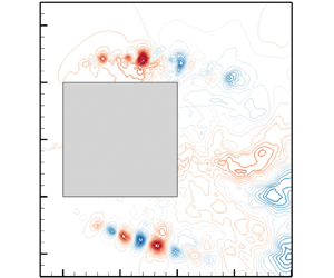
In many turbulent flow conditions, a low-frequency large-amplitude oscillation can be present and can have a strong impact on other coexisting turbulent phenomena, modulating them. One very illustrative example is blood flow in the heart or air flow in the lungs where, according to the phase of the heart beat or of the inhalation/exhalation period, different physical phenomena may take place. Another example is rotating machines, where the turbulence emitted by moving blades strongly depends on its position and thus on the phase of the rotation. This example is intimately connected to a broader category of problems, which are fluid–structure interactions, where mean-flow analyses do not make much sense (in those cases, a change in the reference frame may be needed; see e.g. Shinde & Gaitonde (Reference Shinde and Gaitonde2021)). Also, flows around bluff bodies typically present a strong VS motion where the small-scale turbulent structures evolving on top of them may exhibit different amplitudes, frequencies and spatial locations depending on the phase and thus the position of the large-scale vortices. In figure 1, we present results pertaining to a squared-section cylinder at a Reynolds number  $Re=U_{\infty } D/\nu =22\,000$. In this flow, two very distinct physical mechanisms are at play: periodic VS and Kelvin–Helmholtz (KH) instabilities in the detached shear layers. We can see that the frequency of the former is much lower than the frequencies of the latter. Also, from the snapshots provided in figure 1(b), we can see that, due to the VS phenomenon, the shear layers on the top and bottom of the cylinder slowly oscillate, inducing changes in the dynamics of the KH structures evolving on top of them (see also Brun et al. Reference Brun, Aubrun, Goossens and Ravier2008).

Figure 1. Direct numerical simulation of a squared-section cylinder at  $Re=22\,000$. (a) Spectrum at point $(-0.4,0.63)$ in the shear-layer region. (b) Snapshots of the (spanwise-averaged) pressure field at four different phases, exhibiting the high-frequency KH phenomenon (blue circles) and its dependency on the lower-frequency VS (red circles). The green point represents the probe used in (a). All variables are made non-dimensional with the side of the square and the inflow velocity while the cylinder is centred at $(0,0)$.
We remark that classical techniques such as POD, SPOD and resolvent analyses, although they can certainly identify/reconstruct all the physical structures in a given flow field, elucidating all present physical mechanisms (see e.g. Pickering et al. (Reference Pickering, Rigas, Nogueira, Cavalieri, Schmidt and Colonius2020) where SPOD could reveal lift-up, KH and Orr mechanisms in a turbulent jet or Sieber, Paschereit & Oberleithner (Reference Sieber, Paschereit and Oberleithner2016) and Mendez, Balabane & Buchlin (Reference Mendez, Balabane and Buchlin2019) where classical POD techniques were adapted to provide a multi-scale analysis, isolating several physical mechanisms), they do not manage to describe the phase dependency of small-scale turbulent phenomena. The reason for this is that they all decompose the signal in spatial modes multiplied by a temporal behaviour. This implies that the spatial shape of a particular mode is not allowed to be altered. Indeed, for the squared-section cylinder, we can clearly see the motion of the high-frequency KH structures with VS motion, while classical SPOD and mean-flow resolvent analyses produce fixed spatial structures (see figure 2). Moreover, the SPOD mode shown in figure 2(a) exhibits, mostly in the bottom shear layer, a shadow of the KH structures at different phases of the VS motion, a feature that we would like to mitigate in the present work. We remark that, similarly, those limitations on classical techniques, such as snapshot POD, can also be observed in the case of highly advective flows or wave propagation phenomena, where solutions to those problems, although they may retain their shape, travel through space. In those cases, modified techniques may lead to better results (see e.g. Iollo & Lombardi Reference Iollo and Lombardi2014; Reiss et al. Reference Reiss, Schulze, Sesterhenn and Mehrmann2018; Cagniart, Maday & Stamm Reference Cagniart, Maday and Stamm2019).

Figure 2. Classical SPOD (a) and mean-flow resolvent (b) modes for the flow around a squared-section cylinder, presented in figure 1, at  $\omega =20$. They produce modes that are ‘steady’ and do not oscillate with VS.
The goal of the present article is to extend SPOD and resolvent analyses so that they describe this phase dependency. From an operator-driven point of view, when the phase-dependent dynamics evolves periodically, given by a periodic limit cycle, a linear homogeneous dynamics can be studied using a Floquet-like analysis (Barkley & Henderson Reference Barkley and Henderson1996; Jallas, Marquet & Fabre Reference Jallas, Marquet and Fabre2017; Shaabani-Ardali, Sipp & Lesshafft Reference Shaabani-Ardali, Sipp and Lesshafft2019). In the non-homogeneous case, where an active forcing term (possibly unknown, as in a turbulent configuration) drives the system, a harmonic resolvent analysis (Wereley & Hall Reference Wereley and Hall1990; Padovan, Otto & Rowley Reference Padovan, Otto and Rowley2020) would provide, in a manner similar to that in McKeon & Sharma (Reference McKeon and Sharma2010) and Beneddine et al. (Reference Beneddine, Sipp, Arnault, Dandois and Lesshafft2016), the most energetic input/output modes. Both approaches provide modes that evolve as a function of the phase of the periodic limit cycle, which is what we are looking for. Yet, these approaches are very expensive and the question arises as to whether simpler and cheaper approaches could be designed in the case where a separation of time scales holds between the turbulent component (to be reconstructed) and the periodic motion. As an illustration, we may come back to the case of the squared-section cylinder, where the KH modes exhibit much higher frequencies than the VS one (typically 20 to 30 times higher). In such cases, and as is the objective of this paper, we may develop a simplified approach based on a quasi-steady (QS) approximation, where the high-frequency dynamics adapts instantaneously to a slow periodic oscillation of the system. This allows us to study each phase of the slow movement independently of each other. This approach can be traced back to, for example, the case of the Stokes layer (Von Kerczek & Davis Reference Von Kerczek and Davis1974; Blennerhassett & Bassom Reference Blennerhassett and Bassom2006), where parallel-flow linear stability analyses of each phase were performed independently. In this work, instead of parallel-flow stability analyses, we consider the resolvent analysis. As a result, the reconstruction problem is markedly simplified (and therefore also its cost reduced), since, instead of solving a space/time problem, we only have to solve several spatial ones, one for each considered phase. This analysis is termed QS resolvent analysis.
From the data-driven point of view, we introduce an extended SPOD analysis based on the short-time Fourier transform (STFT) instead of the Fourier transform. This STFT extracts, at a given phase of the slow motion, the local frequency spectrum of the signal, from which the spectral correlation tensor is built, just as in classical SPOD. For this reason, this analysis is referred to as phase-conditioned localized (PCL) SPOD analysis.
The paper is organized as follows. First, in § 2, the theoretical aspects of the PCL-SPOD and QS resolvent analyses are presented. For this, after introducing the Floquet stability theory (for homogeneous solution) and the harmonic resolvent analysis (for the forced solution), we consider the QS approximation, which results in the QS resolvent analysis. Then, we present the STFT and the PCL-SPOD. In § 3, we consider a simple model, a modified version of the linear Ginzburg–Landau equation, where the instability parameter is considered as time dependent and periodic. We illustrate the theory on this simple model, and in particular assess the validity of the QS approximation as a function of the time-scale separation between the solution and the instability parameter. Then, in § 4, we use those techniques to identify and reconstruct the KH structures for the squared-section cylinder case, already presented in figure 1. In order to apply the new tools, the raw velocity/pressure signals of the direct numerical simulation need first to be separated into a periodic (phase-averaged) motion and the remaining turbulent part. This is achieved with a triple decomposition as in (Reynolds & Hussain Reference Reynolds and Hussain1972), (Mezić Reference Mezić2013) and (Arbabi & Mezić Reference Arbabi and Mezić2017).
2. Theory
The goal of this section is to introduce the tools, both operator-driven and data-driven, which aim at capturing high-frequency turbulent phenomena evolving according to the phase of a low-frequency periodic limit cycle. They are introduced with a generic model consisting of a linear periodically time-varying forced equation.
2.1. A generic model
We consider the following generic linear forced system:
 \begin{equation} B \partial_t w + L(t) w = P f(t), \end{equation}
where  $w(t)$ and $f(t)$ represent the state and forcing and $B$,
$B$,  $L(t)$ and $P$ are linear operators. Operator $L(t)$ is a time-periodic operator of fundamental frequency $\omega _0=2{\rm \pi} /T_0$ (representing the effect of the periodic evolution of the phase-averaged component on the fluctuation field), while $f(t)$ is a generic forcing (due in turbulent flows to nonlinear interactions of fluctuations). Here we are particularly interested in the case of high-frequency forcing $\omega _f \gg \omega _0$.
2.1.1. Stability of unforced solutions
It is important for forced systems to determine whether the homogeneous solutions ( $f=0$) are stable or not. This is classically achieved in linear time-periodic systems with a Floquet stability analysis, where we look for solutions of the form $w(t) = \hat {w}(t) {\rm e}^{\sigma t}$, where $\hat {w}(t)$ is a $T_0$-periodic eigenmode and $\sigma$ its complex eigenvalue. If the real part of $\sigma$ is larger than zero, then the eigenmode $\hat {w}(t)$ is said to be Floquet-unstable. By replacing this ansatz in (2.1), we get
 \begin{equation} B \partial_t \hat{w} + \sigma B \hat{w} + L(t) \hat{w} = 0. \end{equation}
The resolution of this system, with, for example, a time-stepping method combined with an eigensolver, leads to the usual Floquet stability analysis (see e.g. Jallas et al. Reference Jallas, Marquet and Fabre2017; Shaabani-Ardali, Sipp & Lesshafft Reference Shaabani-Ardali, Sipp and Lesshafft2017). Another approach (Lazarus & Thomas Reference Lazarus and Thomas2010) that has recently attracted attention in the fluids community (see e.g. Moulin Reference Moulin2020a) is to pose the problem in frequency space by Fourier-decomposing the  $T_0$-periodic solution $\hat {w}(t)$ and operator $L(t)$ as
 \begin{equation} \hat{w}(t) = \lim_{N_h \rightarrow \infty} \sum_{n={-}N_h}^{+ N_h} \hat{w}^{(n)} \exp({{\rm i} n \omega_0 t}), \quad L(t) = \lim_{N_h \rightarrow \infty} \sum_{n={-}N_h}^{{+}N_h} L^{(n)} \exp({{\rm i} n \omega_0 t}). \end{equation}
Substituting this expression in (2.2), we obtain the following infinite-matrix eigenvalue/eigenvector problem:
 \begin{equation} ( \mathcal{H} + \sigma \mathcal{B} ) \hat{\mathcal{W}} = 0, \end{equation}
where  $\mathcal {B}$ is an infinite block-diagonal matrix with $B$ matrices on the diagonal, $\mathcal {H}$ is the so-called Hill matrix (see Lazarus & Thomas Reference Lazarus and Thomas2010),
 \begin{equation} \mathcal{H} = \begin{bmatrix} \ddots & \vdots & \vdots & \vdots & \unicode{x22F0} \\ \cdots & L^{(0)} - \mathrm{i} \omega_0 B & L^{({-}1)} & L^{({-}2)} & \cdots \\ \cdots & L^{(1)} & L^{(0)} & L^{({-}1)} & \cdots \\ \cdots & L^{(2)} & L^{(1)} & L^{(0)} + \mathrm{i}\omega_0 B & \cdots \\ \unicode{x22F0} & \vdots & \vdots & \vdots & \ddots \end{bmatrix}, \end{equation}
and the eigenvector
 \begin{equation} \hat{\mathcal{W}}=(\cdots, \hat{w}^{({-}1)}, \hat{w}^{(0)}, \hat{w}^{(1)}, \ldots)^{\rm T} \end{equation}
is a column vector concatenating all harmonics of the time-periodic mode  $\hat {w}(t)$. This is the so-called Floquet–Hill theory, which allows us to see the Floquet eigenvalue/eigenvector problem as a usual (yet infinite) matrix eigenproblem.
2.1.2. Forced solutions
In the case where the system is Floquet-stable, all homogeneous solutions decay to zero for  $t \rightarrow \infty$. Then, for a given forcing $f(t)$, there exists a unique sustained solution $w(t)$. We consider general forcing terms of the form $f(t) = \sum _k \hat {f}(\omega _{f,k},t) \exp ({{\rm i} \omega _{f,k} t})$, with different frequencies $\omega _{f,k}$ and envelopes $\hat {f}(\omega _{f,k},t)$ that are all $T_0$-periodic. By linearity, we may then look for solutions under the form $w(t) = \sum _k \hat {w}(\omega _{f,k},t) \exp ({{\rm i} \omega _{f,k} t})$, where the envelopes $\hat {w}(\omega _{f,k},t)$ are also $T_0$-periodic. Hence, without loss of generality, we may consider the single-frequency forcing case
 \begin{equation} f(t) = \hat{f}(t) \exp({\mathrm{i} \omega_f t}), \quad w(t)=\hat{w}(t) \exp({\mathrm{i}\omega_f t}), \end{equation}
where the envelopes  $\hat {f}(t)$ and $\hat {w}(t)$ are both $T_0$-periodic. Inserting this assertion into (2.1), we have
 \begin{equation} B \partial_t \hat{w} + \mathrm{i} \omega_f B \hat{w} + L(t) \hat{w} = P\hat{f}. \end{equation}
If  $\hat {f}$ is available, the solution $\hat {w}$ may be obtained by time-stepping the system until the transient has gone away (the system is Floquet-stable). Alternatively, similar to before, we may pose this problem in frequency space by expanding the various terms in their Fourier series and rewrite the system (2.8) as
 \begin{equation} ( \mathrm{i} \omega_f \mathcal{B} + \mathcal{H}) \hat{\mathcal{W}} = \mathcal{P} \hat{\mathcal{F}}. \end{equation}
Here  $\mathcal {P}$ is a block-diagonal matrix containing the matrices $P$ and $\hat {\mathcal {F}}$ is the forcing term with all its time harmonics:
 \begin{equation} \hat{\mathcal{F}}=(\cdots, \hat{f}^{({-}1)}, \hat{f}^{(0)}, \hat{f}^{(1)}, \ldots)^{\rm T}, \quad \hat{f}(t) = \lim_{N_h \rightarrow \infty} \sum_{n={-}N_h}^{+ N_h} \hat{f}^{(n)} \exp({{\rm i} n \omega_0 t}). \end{equation}
The advantage of this approach is to show that the forced solution can be obtained by a usual (yet infinite) matrix inverse, which is called the harmonic resolvent operator. The latter operator therefore characterizes the input/output dynamics.
2.2. Resolvent analyses
Although (2.8) (or alternatively (2.9)) does provide the exact solution, given a known forcing term  $f(t) = \hat {f}(t) \exp ({\mathrm {i} \omega _f t})$, we are interested in situations where the solution is primarily selected by the linear input/output operator and only marginally by the actual forcing. Such conditions are met when the harmonic resolvent operator is of low rank, which is a common situation in fluid mechanics due to the existence of strong instability mechanisms. For this purpose, as in McKeon & Sharma (Reference McKeon and Sharma2010) and Beneddine et al. (Reference Beneddine, Sipp, Arnault, Dandois and Lesshafft2016), we first (§ 2.2.1) introduce the singular values/singular vectors of the harmonic resolvent operator, which characterize the rank of the operator and the predominant responses. Then (§ 2.2.2), we focus on the case where the frequency of the forcing $\omega _f$ is much higher than the frequency of the limit cycle $\omega _0$ and introduce a QS approximation, which reduces the problem to a classical resolvent analysis around a time instant of the low-frequency motion.
2.2.1. Harmonic resolvent analysis
Equation (2.9) establishes an input/output relation between a forcing term  $\hat {\mathcal {F}}$ and the solution $\hat {\mathcal {W}}$. Noting the harmonic resolvent operator $\mathcal {R}(\omega _f) = (\mathrm {i} \omega _f \mathcal {B} + \mathcal {H})^{-1} \mathcal {P}$ so that $\hat {\mathcal {W}} = \mathcal {R} \hat {\mathcal {F}}$ (see Wereley & Hall Reference Wereley and Hall1990; Padovan et al. Reference Padovan, Otto and Rowley2020), we look for the most energetic input/output dynamics, maximizing the following energy gain over $\hat {\mathcal {F}}$:
 \begin{equation} \gamma^{2}(\omega_f) = \frac{\int_0^{T_0} \| \hat{w} (t) \|_{\varOmega}^{2} \,{\rm d}t}{\int_0^{T_0} \| \hat{f} (t) \|_{\varOmega}^{2} \,{\rm d}t} \underbrace{=}_{\mbox{Parseval}} \frac{ \sum_i \| \hat{w}_i \|_{\varOmega}^{2} }{ \sum_i \| \hat{f}_i \|_{\varOmega}^{2} } = \frac{\sum_i\hat{w}_i^{*} M_\varOmega \hat{w}_i }{ \sum_i\hat{f}_i^{*} M_\varOmega \hat{f}_i}=\frac{ \hat{\mathcal{W}}^{*} \mathcal{M} \hat{\mathcal{W}} }{\hat{\mathcal{F}}^{*} \mathcal{M} \hat{\mathcal{F}} }, \end{equation}
subjected to  $\hat {\mathcal {W}} = \mathcal {R}\hat {\mathcal {F}}$. The infinite matrix $\mathcal {M}$ is block-diagonal with $M_\varOmega$ matrices on the diagonal, $M_\varOmega$ being linked to the energy norm $\| u \|_{\varOmega }^{2} = \sqrt { \langle u , u \rangle _{\varOmega }}$ and $\langle u , v \rangle _{\varOmega } = \int _{\varOmega } u^{*} v \,{\rm d}\kern0.7pt\boldsymbol {x}$. This then leads to the following (infinite-matrix) eigenproblem:
 \begin{equation} \mathcal{R}^{*} \mathcal{M} \mathcal{R} \hat{\mathcal{F}}_i (\omega_f) = \gamma_i^{2}(\omega_f) \mathcal{M} \hat{\mathcal{F}}_i (\omega_f), \end{equation}
where  $\mathcal {R}^{*}$ is the transconjugate of $\mathcal {R}$. The normalized vectors $\hat {\mathcal {F}}_i$ are the optimal forcings such that $\mathcal {F}^{*}\mathcal {M}\mathcal{F}=\delta _{ij}$, for each frequency. The corresponding unit-norm optimal responses are given by the relation $\hat {\mathcal {\varPsi }}_i(\omega _f) = \gamma _i^{-1}\mathcal {R} \hat {\mathcal {F}}_i(\omega _f)$.
Similarly to Beneddine et al. (Reference Beneddine, Sipp, Arnault, Dandois and Lesshafft2016), it may be shown that, if  $\gamma _0(\omega _f) |\hat {\mathcal {F}}_0(\omega _f)^{*}\mathcal {M} \hat {\mathcal {F}}| \gg \gamma _i(\omega _f) |\hat {\mathcal {F}}_i(\omega _f)^{*}\mathcal {M} \hat {\mathcal {F}}|$ for $i \geq 1$ (which is the case if the harmonic resolvent operator is strictly rank one, $\gamma _0(\omega _f)>\gamma _1(\omega _f)=0$), then
 \begin{equation} \hat{\mathcal{W}}(\omega_f) {\rm e}^{{\rm i} \omega_f t} \approx A \hat{\mathcal{\varPsi}}_0(\omega_f) {\rm e}^{{\rm i} \omega_f t}, \end{equation}
with  $A=\gamma _0(\omega _f) [\hat {\mathcal {F}}_0(\omega _f)^{*}\mathcal {M} \hat {\mathcal {F}}]$. This result states that the spatial structure of the response is at all times proportional to the dominant singular mode of the harmonic resolvent operator. Stochastic arguments as in Towne et al. (Reference Towne, Schmidt and Colonius2018) may also be provided to justify such a result.
2.2.2. Quasi-steady resolvent analysis
If the envelope of the forcing  $\hat {f}(t)$ evolves on the slow time scale $T_0$ and if $\omega _0 \ll \omega _f$, then it is reasonable to simplify the term $B \partial _t \hat {w}$ in (2.8) (as done in Von Kerczek & Davis (Reference Von Kerczek and Davis1974) for Stokes layer analysis), which should be small with respect to ${\rm i}\omega _f B \hat {w}$. We therefore end up with the following simpler equation:
 \begin{equation} \mathrm{i} \omega_f B \hat{w}(t) + L(t) \hat{w}(t) = P \hat{f}(t). \end{equation}
There are actually conditions for this approximation to hold. More insight can be gained by considering the system involving the Floquet–Hill matrix (2.9). Yet, for brevity, we have put these arguments in Appendix A.
Equation (2.14) is the QS approximation, whose solution can be recast in the following form:
 \begin{equation} \hat{w}(t) = R_t \hat{f}(t), \end{equation}
where  $R_t=( \mathrm {i} \omega _f B + L(t) )^{-1} P$ is the QS resolvent operator. The solution at each time $t_1$, $\hat {w}(t_1)$, is therefore independent of the solution at any other time $t_2$, $\hat {w}(t_2)$. We see that each time instant (or phase, within the period $[0,T_0)$) can be analysed separately.
Under the QS approximation given by (2.14), we then look for the most energetic input/output dynamics, maximizing the following energy gain over  $\hat {f}$ (McKeon & Sharma Reference McKeon and Sharma2010; Beneddine et al. Reference Beneddine, Sipp, Arnault, Dandois and Lesshafft2016):
 \begin{equation} \gamma'^{2}(\omega_f,t) = \frac{ \| \hat{w} \|_{\varOmega}^{2} }{ \| \hat{f} \|_{\varOmega}^{2} } = \frac{\hat{w}^{*} M_\varOmega \hat{w} }{ \hat{f}^{*} M_\varOmega \hat{f}}, \end{equation}
under the constraint  $\hat {w}=R_t \hat {f}$. This leads to the following (finite-matrix) eigenproblem:
 \begin{equation} R^{*}_t M_\varOmega R_t \hat{f}'_i (\omega_f,t) = \gamma_i'^{2}(\omega_f,t) M_\varOmega \hat{f}'_i (\omega_f,t), \end{equation}
where  $R^{*}_{t}$ is the transconjugate of the resolvent $R_{t}$. The normalized vectors $\hat {f}'_i (\omega _f,t)$ are the optimal forcings such that $\hat {f}_i'^{*} M_\varOmega \hat {f}_j'=\delta _{ij}$, for each frequency and phase. The corresponding optimal fluctuations are given by the relation $\hat {\psi }'_i(\omega _f,t) = \gamma _i'(\omega _f,t)^{-1}R_{t} \hat {f}'_i(\omega _f,t)$.
Similarly to the previous section, it may be shown that, in the presence of a nearly rank-one  $R_t$ operator,
 \begin{equation} \hat{w}(\omega_f,t) {\rm e}^{{\rm i} \omega_f t} \approx A(t) \hat{\psi}'_0(\omega_f,t) {\rm e}^{{\rm i} \omega_f t}, \end{equation}
with  $A$ as a complex constant. This result states that the spatial structure of the high-frequency response is at all times proportional to the dominant singular mode of the QS resolvent. Stochastic arguments as in Towne et al. (Reference Towne, Schmidt and Colonius2018) may also be provided to obtain such a result.
2.3. Data-driven approach
In this section, we address the problem of identifying from data high-frequency structures evolving on slowly varying periodic limit cycles. This analysis is based on the STFT, which is used as input to define an extended version of SPOD. This approach is termed PCL-SPOD.
2.3.1. Short-time Fourier transform analysis
The QS approach is well suited for the determination, from knowledge of the governing equations, of high-frequency fluctuations at every phase within a slowly varying limit cycle. In this discussion, we look at the data-driven side where, from the raw signal  $w(t)$, we try to answer this same question and identify within the signal high-frequency patterns that behave as $\hat {w}_W (t) {\rm e}^{ \mathrm {i} \omega t}.$ Again, the envelope $\hat {w}_W (t)$ evolves on a slow time scale of order $T_0$ while the exponential is based on a rapid frequency $\omega \gg \omega _0$. For this, we consider the signal around a phase $t$ by multiplying it by a window function $W(\tau -t)$, leading to a PCL signal:
 \begin{equation} w_{W}(\tau,t) = W(\tau - t) w(\tau), \end{equation}
where the notation  $(\cdot )_W$ represents the windowed function. The window function $W(\eta )$ is chosen to have a compact support of duration $\Delta T$, with $W(\eta ) > 0$ for $\eta \in (-\Delta T / 2, \Delta T /2)$ and $0$ elsewhere, and unit integral over $\eta$. A common example of such a function is the Hann window, shown in figure 3(a). If we want to investigate the frequency content of the signal in the vicinity of the phase $t$, we Fourier-transform this quantity:
 \begin{equation} \hat{w}_{W}(\omega,t) = \int_{-\infty}^{+\infty} w_W(\tau,t) {\rm e}^{- \mathrm{i} \omega \tau}\,{\rm d}\tau = \int_{-\infty}^{+\infty} W(\tau-t) w(\tau) \exp({- \mathrm{i} \omega \tau})\,{\rm d}\tau. \end{equation}
This is exactly the STFT or windowed Fourier transform (see Griffin & Lim Reference Griffin and Lim1984).

Figure 3. (a) Normalized Hann window  $W(\eta ) := ({1+\cos (2 {\rm \pi}\eta / \Delta T)})/{\Delta T}$ within $-1/2 \leq \eta /\Delta T \leq 1/2$ and zero outside. (b) Fourier transform $\hat {W}(\omega _{\eta }) = {\sin (\Delta T \omega _{\eta }/2)}/({ (\Delta T\omega _{\eta }/2)(1- (\Delta T \omega _{\eta }/2 {\rm \pi})^{2})})$.
For simplicity, let us choose a signal of the form  $w(t) = \hat {w}(t) \exp ({\mathrm {i} \omega _f t})$, with $|\omega _f|\gg \omega _0$. For the case where several frequencies $\omega _{f,k}$ are present, the arguments given in the following also apply. Since $\hat {w}(t)$ is a slowly evolving envelope on the time scale $T_0$, if $\Delta T \ll T_0$, then $\hat {w}(t)$ is nearly constant within the window $W(t-\tau )$ and may be taken out of the integral:
 \begin{align} \hat{w}_{W}(\omega,t) &= \int_{-\infty}^{+\infty} W(\tau-t) \hat{w}(\tau) \exp({\mathrm{i} \omega_f \tau}) \exp({-{\rm i} \omega \tau}) \,{\rm d}\tau\nonumber\\ & \approx \hat{w}(t) \int_{-\infty}^{+\infty} W(\tau-t) \exp({\mathrm{i} (\omega_f-\omega) \tau})\,{\rm d}\tau\nonumber\\ &\approx\hat{w}(t) \exp({\mathrm{i} (\omega_f-\omega) t}) \int_{-\infty}^{+\infty} W(\tau') \exp({-\mathrm{i} (\omega-\omega_f) \tau'}) \,{\rm d}\tau' \nonumber\\ &\approx\hat{w}(t) \exp({\mathrm{i} (\omega_f-\omega) t}) \hat{W}(\omega-\omega_f). \end{align}
This shows that the STFT of the signal is approximately proportional to  $\hat {w}_W \approx \hat {w}(t) \exp ({\mathrm {i} (\omega _f-\omega ) t})$, with a constant of proportionality equal to the Fourier transform of the window function $\hat {W}(\omega -\omega _f)$. The latter is shown in figure 3(b) for the Hann window.
From this, we can see that we have two cases:
(i) If $\omega$ is close to $\omega _f$ but still satisfying $|\omega - \omega _f|/\omega _0 \ll (\Delta T/T_0)^{-1}$, then the constant $\hat {W}(\omega -\omega _f)$ is close to $1$. In such a case, we have
(2.22)and the actual frequency of the structure\begin{equation} \hat{w}_W(t) \approx \hat{w}(t) \exp({\mathrm{i} (\omega_f-\omega) t}), \end{equation}$\omega _f$ may be determined by looking for the frequency $\omega$ for which $\hat {w}_W(t)$ is $T_0$-periodic. In such a case, we finally have $\hat {w}_W(t) {\rm e}^{\mathrm {i} \omega t} \approx \hat {w}(t) {\rm e}^{\mathrm {i} \omega _f t}$, which shows that the STFT accurately identifies the spatio-temporal structure. In practice, the STFT $\hat {w}_W(\omega,t)$ is computed using a fast Fourier transform algorithm, which provides $\hat {w}_W(\omega,t)$ on a frequency grid. This first scenario corresponds to the case where a frequency $\omega$ on that grid approximately corresponds to $\omega _f$. Note that when the time resolution is very high, $\Delta T/T_0 \ll 1$, the range of frequencies $|\omega - \omega _f|$ over which $\hat {W}(\omega -\omega _f)$ remains equal to $1$ becomes very large, which translates to the fact that the frequency resolution $\Delta \omega =2{\rm \pi} /\Delta T$ in the fast Fourier transform becomes very poor.
$\omega$ is close to $\omega _f$ but still satisfying $|\omega - \omega _f|/\omega _0 \ll (\Delta T/T_0)^{-1}$, then the constant $\hat {W}(\omega -\omega _f)$ is close to $1$. In such a case, we have
(2.22)and the actual frequency of the structure\begin{equation} \hat{w}_W(t) \approx \hat{w}(t) \exp({\mathrm{i} (\omega_f-\omega) t}), \end{equation}$\omega _f$ may be determined by looking for the frequency $\omega$ for which $\hat {w}_W(t)$ is $T_0$-periodic. In such a case, we finally have $\hat {w}_W(t) {\rm e}^{\mathrm {i} \omega t} \approx \hat {w}(t) {\rm e}^{\mathrm {i} \omega _f t}$, which shows that the STFT accurately identifies the spatio-temporal structure. In practice, the STFT $\hat {w}_W(\omega,t)$ is computed using a fast Fourier transform algorithm, which provides $\hat {w}_W(\omega,t)$ on a frequency grid. This first scenario corresponds to the case where a frequency $\omega$ on that grid approximately corresponds to $\omega _f$. Note that when the time resolution is very high, $\Delta T/T_0 \ll 1$, the range of frequencies $|\omega - \omega _f|$ over which $\hat {W}(\omega -\omega _f)$ remains equal to $1$ becomes very large, which translates to the fact that the frequency resolution $\Delta \omega =2{\rm \pi} /\Delta T$ in the fast Fourier transform becomes very poor.(ii) If the frequency
$\omega$ is very different from $\omega _f$, such that $|\omega - \omega _f|/\omega _0 \gtrapprox (\Delta T/T_0)^{-1}$, $\hat {W}(\omega -\omega _f)$ tends to zero, making $\hat {w}_W \rightarrow 0$. For far enough frequencies, the STFT therefore filters out the signal.


Those remarks are especially important in the case where several different frequencies  $\omega _{f,k}$ are present in the signal, $w(t) = \sum _k \hat {w}(\omega _{f,k},t) \exp ({{\rm i} \omega _{f,k} t})$. In that case, $\hat {w}_W(\omega,t)$, computed at $\omega$, will be influenced by nearby frequencies $\omega _{f,k}$ in the interval $(\omega -{\rm \pi} /\Delta T, \omega +{\rm \pi} /\Delta T)$. For this reason, if we want to isolate specific frequencies $\omega _{f,k}$ with $\hat {w}_W$, a large $\Delta T$ must be chosen, but still with the constraint $\Delta T \ll T_0$, so that the phase dependency $\hat {w}_W(t)$ is not entirely lost (time resolution). A further discussion on this compromise is provided in the next section on a numerical problem. We also point out that if two distinct frequencies $\omega _{f,k}$ are close to each other, it may no longer be possible to distinguish their modes $\hat {w}(\omega _{f,k},t)$.
2.3.2. Phase-conditioned localized SPOD analysis
In turbulent configurations, we are often interested in the stochastic framework, where several realizations of the flow are considered. From the data-driven point of view, this is accounted for by a POD analysis of the realizations of the STFT,  $\hat {w}_W$. Since this approach considers the signal conditioned by the phase of the low-frequency motion of the dynamics and since each phase is evaluated locally and independently of the other phases (due to the QS considerations), we refer to it as PCL-SPOD analysis.
This PCL-SPOD analysis is very closely related to the classical SPOD (see Towne et al. Reference Towne, Schmidt and Colonius2018) where, from a practical point of view, the only difference is that we perform the POD with modes issuing from a STFT performed on a small interval of length  $\Delta T$ rather than from a Fourier transform or STFT performed on the full length of the bin. Basically, we are trying to maximize over $\hat {\phi }(x,\omega,t)$ the energy:
 \begin{equation} \lambda^{2}(\omega,t) = \frac{E \left[ \left| \left \langle \hat{w}_W (x,\omega,t) , \hat{\phi}(x,\omega,t) \right \rangle_{\varOmega} \right|^{2} \right] }{ \left \langle \hat{\phi}(x,\omega,t) , \hat{\phi}(x,\omega,t) \right \rangle_{\varOmega} }, \end{equation}
where  $\langle u , v \rangle _{\varOmega } = \int _{\varOmega } u^{*} v \,{\rm d}\kern0.06pt \boldsymbol {x}$ is the energy inner product. The quantity $\hat {w}_W (x,\omega,t)$ is stochastic and depends on the realization. The notation $E[\cdot ]$ is the expected value operator, and is defined to be an average over all realizations, each of size $T_0$. This problem is equivalent to solving the following eigenvalue/eigenvector problem:
 \begin{equation} \int_{\varOmega} \boldsymbol{\mathsf{S}}(\boldsymbol{x},\boldsymbol{x}',\omega,t) \hat{\phi}_i(\boldsymbol{x}',\omega,t) \, {\rm d}\kern0.06pt \boldsymbol{x}' = \lambda_i(\omega,t)^{2} \hat{\phi}_i(\boldsymbol{x},\omega,t), \end{equation}
where  $\boldsymbol{\mathsf{S}}(\boldsymbol {x},\boldsymbol {x}',\omega,t)$ is the cross-spectral tensor, evaluated at phase (or time) $t$, and is defined as
 \begin{equation} \boldsymbol{\mathsf{S}}(\boldsymbol{x},\boldsymbol{x}',\omega,t) = E \left[\hat{w}_W(\boldsymbol{x},\omega,t) \hat{w}_W^{*}(\boldsymbol{x}',\omega,t) \right]. \end{equation}
We believe that, in a similar way that classical SPOD is related to space/time POD (Towne et al. Reference Towne, Schmidt and Colonius2018), this PCL-SPOD is related to the conditional space/time of Schmidt & Schmid (Reference Schmidt and Schmid2019) and Hack & Schmidt (Reference Hack and Schmidt2021) when the conditioning signals are the phases of the lower-frequency dynamics. A proof of this is given in Appendix B.
2.3.3. Phase-average and numerical implementation of PCL-SPOD
We now discuss precisely how to estimate the operator  $E[\cdot ]$. Since the low-frequency oscillation is $T_0$-periodic, we consider here $N_p$ individual periods as independent realizations of the fluid flow. In this context, the expected value operator is written as
 \begin{equation} E[w] (t) \equiv \left \langle w \right \rangle (t) = \frac{1}{N_p} \sum_{k=1}^{N_p} w(x,t+kT_0), \quad \text{for} \ t \in [0,T_0). \end{equation}
This is precisely the definition of the phase average  $\langle \cdot \rangle$ introduced by Reynolds & Hussain (Reference Reynolds and Hussain1972), where they also looked for capturing turbulent oscillations around a periodic wave of period $T_0$ at different phases of the period $[0,T_0)$. We remark that this operator readily considers the signal $w(t)$ at the same phases of the slowly varying dynamics since we evaluate the signal $w(t)$ at time instants modulo $T_0$. With that in mind, the spectral tensor $\boldsymbol{\mathsf{S}}$ defined in (2.25) can be approximated as
 \begin{equation} \boldsymbol{\mathsf{S}}(\boldsymbol{x},\boldsymbol{x}',\omega,t) = \frac{1}{N_p} \sum_{k=1}^{N_p} \hat{w}_W(\omega,t+kT_0) \hat{w}_W^{*}(\omega,t+kT_0) \equiv \hat{\boldsymbol{\mathsf{W}}}(\omega,t) \hat{\boldsymbol{\mathsf{W}}}(\omega,t)^{*}, \end{equation}
where  $\hat {\boldsymbol{\mathsf{W}}}(\omega,t)$ is a matrix containing the STFT (normalized by $1/\sqrt {N_p}$) of all the periods considered for a given phase $t$ and frequency $\omega$. In figure 4, we provide a schematic representation of how this matrix $\hat {\boldsymbol{\mathsf{W}}}(\omega,t)$ is computed from data. Also, from now on, we no longer consider the problem posed in the continuous framework, and we consider that all the space integrals presented so far are given, in a discrete formalism, by the matrix $M_{\varOmega }$, containing the integration weights. In this framework, the PCL-SPOD problem is rewritten as
 \begin{equation} \hat{\boldsymbol{\mathsf{W}}} \hat{\boldsymbol{\mathsf{W}}}^{*} M_{\varOmega} \hat{\phi}(\omega,t) = \lambda^{2} (\omega,t) \hat{\phi}(\omega,t). \end{equation}
It is worth mentioning that this problem involves finding the eigenvalues/eigenvectors of a large dense matrix  $\hat {\boldsymbol{\mathsf{W}}} \hat {\boldsymbol{\mathsf{W}}}^{*}$. Instead, we solve the following eigenvalue/eigenvector problem:
 \begin{equation} \hat{\boldsymbol{\mathsf{W}}}^{*} M_{\varOmega} \hat{\boldsymbol{\mathsf{W}}} \hat{\boldsymbol{y}}(\omega,t) = \lambda^{2} (\omega,t) \hat{\boldsymbol{y}}(\omega,t), \end{equation}
involving a much smaller matrix  $\hat {\boldsymbol{\mathsf{W}}}^{*} M_{\varOmega } \hat {\boldsymbol{\mathsf{W}}}$, whose dimension is the number of bins. The PCL-SPOD mode can then be recovered as $\hat {\phi } = \lambda ^{-1} \hat {\boldsymbol{\mathsf{W}}} \hat {\boldsymbol {y}}$.

Figure 4. Schematic representation of how to compute the PCL-SPOD from data of a single run  $w(t)$, divided in $N_p$ periods (or bins). This is equivalent to the Welch algorithm (Welch Reference Welch1967) where no overlap between the bins is used, in order to keep the phase dependency.
3. Application to the case of modified linear forced Ginzburg–Landau model
In this section, we illustrate the theory on a simple and well-understood model, the linear Ginzburg–Landau equation. This equation has served as a prototype for modelling and understanding fluid dynamics instabilities in parallel and non-parallel wake flows (see e.g. Roussopoulos & Monkewitz Reference Roussopoulos and Monkewitz1996; Cossu & Chomaz Reference Cossu and Chomaz1997; Chomaz, Huerre & Redekopp Reference Chomaz, Huerre and Redekopp1988) and for the design of control strategies (see Lauga & Bewley Reference Lauga and Bewley2003; Bagheri et al. Reference Bagheri, Henningson, Hoepffner and Schmid2009; Chen & Rowley Reference Chen and Rowley2011). For this simple one-dimensional model, we are able to perform all the analyses presented in the previous section, compare them and also assess the QS approximation. Here,  $B=P=I$ are identity matrices and
 \begin{equation} L = U \partial_x - \nu \partial_{xx} - \mu \quad \text{and} \quad \mu = \mu_0-c_u^{2} + \mu_2 \frac{x^{2}}{2}, \end{equation}
with  $|w(x\rightarrow \pm \infty,t)| \rightarrow 0$. This model mimics an open flow around a bluff body, which is characterized by downstream advection $U$, diffusion $\nu$ and an instability term ( $\mu _0,c_u,\mu _2$) standing for production of perturbations due to shear in the recirculation region. The spatial extent of the unstable region is governed by $\mu _2$: when considering a parallel ( $\mu _2=0$), unforced ( $f(t)=0$) case, a solution of the form $w=\hat {q} \exp ({ \mathrm {i} k x - \mathrm {i} \omega t})$ is unstable for wavenumbers in the interval $k \in (c_u-\sqrt {\mu _0},c_u+\sqrt {\mu _0})$ (see Bagheri et al. Reference Bagheri, Henningson, Hoepffner and Schmid2009), showing that $\mu _0=0$ is the critical value for local temporal instabilities, above which waves of size around $k=c_u$ are amplified. For the non-parallel case, $\mu _2\neq 0$, the stability of the system can be interrogated by the ansatz $w=\hat {q}(x) {\rm e}^{\lambda t}$, leading to
 \begin{equation} \lambda_n = \mu_0-c_u^{2} - (U^{2}/4\nu) - (n+1/2)h, \quad \hat{q}_n = \exp({(U/2\nu)x - \chi^{2} x^{2}/2})H_n(\chi x), \end{equation}
where  $h=\sqrt {- 2 \mu _2 \nu }$ and $\chi =(-\mu _2/2\nu )^{1/4}$. The system is thus globally stable when the real part of $\lambda _0$ is less than zero, or $\mu _0 < \mu _{0,cr}$. For the following set of parameters (Bagheri et al. Reference Bagheri, Henningson, Hoepffner and Schmid2009):
 \begin{equation} c_u = 0.1, \quad \mu_2 ={-} 0.01, \quad U = 2 + 2 {\rm i} c_u, \quad \nu = 1 - {\rm i}, \end{equation}
the critical value is  $\mu _{0,cr}\approx 0.4827$. However, although the system is stable, it may strongly amplify external noise (pseudo-resonance phenomenon due to the non-normality of the linear operator). To quantify this behaviour, we resort to resolvent analysis where we suppose that both the forcing term and the solution can be written as $f(x,t)=\hat {f}(x) {\rm e}^{{\rm i} \omega t}$ and $w(x,t)=\hat {w}(x) {\rm e}^{{\rm i} \omega t}$, and maximize the energy gain $\gamma '(\omega )=\| \hat {w} \|_{\varOmega } / \| \hat {f} \|_{\varOmega }$, leading to the results shown in figure 5. We can see that those gains can be very high, even for subcritical values of $\mu _0$.

Figure 5. Optimal energy amplifications  $\gamma _{i=1}'(\omega )$ by the linear Ginzburg–Landau equation, as a function of the frequency $\omega$ for a few values of $\mu _0<\mu _{0,cr}=0.4827$.
The discretization of the spatial operators in the Ginzburg–Landau model is handled with second-order P2 continuous elements using the code FreeFEM (Hecht Reference Hecht2012), the source code used here having been adapted from Sipp, de Pando & Schmid (Reference Sipp, de Pando and Schmid2020). The mesh is uniform with  $\Delta x = 0.05$ and extends over $x \in [-30,100]$, well enough for discretizing the regions where the instability term is positive ( $\mu (x)>0$ roughly for ${|x| \leq 20}$). The optimal forcings/responses were obtained using Arpack (Lehoucq, Sorensen & Yang Reference Lehoucq, Sorensen and Yang1998) combined with a direct LU-solver (Amestoy et al. Reference Amestoy, Buttari, L'Excellent and Mary2019) for the matrix inverses.
In order to obtain a model whose dynamics varies periodically, we choose to make  $\mu _0$ time-dependent in the following manner:
 \begin{equation} \mu_0(t) = \bar{\mu}_0 + A_{\mu_0} \sin(\omega_0 t - {\rm \pi}/2), \end{equation}
where  $\bar {\mu }_0$ is the average value, $A_{\mu _0}$ is the amplitude and $\omega _0$ is the frequency for the oscillation of $\mu _0 (t)$. We may expect that the dynamics presented in figure 5 can be recovered at all phases within $t \in [0,T_0)$ for a sufficiently low oscillation frequency $\omega _0 \ll \omega$. This is essentially the QS approach, which is investigated in the following.
3.1. Floquet stability analysis
In this section, we present the Floquet stability analysis. This analysis is carried out using the Floquet–Hill theory. The eigenvalue problem (2.9) is solved using a shift-and-invert strategy (the matrix inverses being handled with the sparse LU solver), associated with an Arnoldi method. The number of harmonics considered was  $N_h=60$, corresponding to a frequency discretization ranging from $-0.94$ to $0.94$. In figure 6(a), we provide the Floquet spectrum for the parameters $\bar {\mu }_0 = 0.4$ and $A_{\mu _0}=0.05$, which shows that all the modes present are stable.

Figure 6. (a) Floquet spectrum for the case  $\bar {\mu }_0=0.4$, $A_{\mu _0}=0.05$ and $\omega _0=2 {\rm \pi}\times 0.0025 \approx 0.016$. This frequency is low in comparison with the peak of the resolvent curve $\omega \in (-0.5, -0.4)$ in figure 5. (b) A zoom for $\mathrm {Im}\{ \sigma \} \in (0,\omega _0)$.
One interesting feature shown in this figure is the  $\omega _0$-periodicity of the spectrum. To understand this feature, we rewrite the eigensolution $w$ as
 $$\begin{gather} w(t) = {\rm e}^{\sigma t} \underbrace{\sum_n \hat{w}_n \exp({\mathrm{i} n \omega_0 t})}_{\hat{w}(t)} = \exp({ (\sigma + \mathrm{i} m \omega_0) t}) \sum_n \hat{w}_n \exp({\mathrm{i} (n-m) \omega_0 t}) \nonumber\\ = {\rm e}^{ \sigma_m t } \underbrace{ \sum_n \hat{w}_{n+m} \exp({\mathrm{i} n \omega_0 t})}_{\text{shifted }{\hat{w}}(t)}. \end{gather}$$
Hence, if a mode  $\hat {\mathcal {W}}=(\cdots, \hat {w}_{-1}, \hat {w}_0, \hat {w}_{+1}, \ldots )$ is an eigenvector with eigenvalue $\sigma$, so is $\hat {\mathcal {W}}_m=(\cdots, \hat {w}_{m-1}, \hat {w}_m, \hat {w}_{m+1}, \ldots )$ with eigenvalue $\sigma _m = \sigma + \mathrm {i} m \omega _0$. We remark that the property, although valid theoretically, may not fully hold when truncating the series representation in (2.7a,b) to $N_h$ harmonics, since, for some $m$, the mode $\hat {\mathcal {W}}_m$ may not be well represented with the considered harmonics.
Also, we verified that for other values of  $\bar {\mu }_0$, $A_{\mu _0}$ and $\omega _0$, the system remains Floquet-stable. In the following, we use the set of parameters:
 \begin{equation} \omega_0 = 2 {\rm \pi}\times 0.0025 \approx 0.016, \quad \bar{\mu}_0 = 0, \quad A_{\mu_0}=0.45. \end{equation}
3.2. Single-frequency forcing case
We consider the single-frequency forcing case,  $f(t) = \hat {f}(t) {\rm e}^{{\rm i} \omega _{f} t}$, for which the solution can be sought under the form $w(t) = \hat {w}(t) {\rm e}^{{\rm i} \omega _{f} t}$. The latter is computed by solving the linear system involved in (2.9) with the direct LU solver. In figure 7, we provide the solution for the case $\omega _f = - 30 \omega _0 \approx -0.47$, near the peak of the energy gain curve in figure 5, and a constant-in-time envelope $\hat {f}(x,t)=g(x)$, where $g(x)=\exp ({-(x-x_f)^{2}/\sigma _x^{2}})$ is a spatial Gaussian localized at $x_f=-11$ and of width $\sigma _x=0.4$. In figure 7(a), we can see that the instability parameter $\mu _0(t)$ presents large values around $t/T_0 \approx 0.5$. In figure 7(b) we show the real part of the forcing term $f(t)=g(x)\exp ({\mathrm {i} \omega _f t})$, which shows that the envelope is constant over the interval $t/T_0 \in [0,1)$ and that the forcing frequency $\omega _f$ is high. In figure 7(c) we show the solution (real part) in the $(x,t)$ plane, with a snapshot at $t/T_0=0.5$ in figure 7(e). We can see that it has a similar oscillatory behaviour to the forcing term but, now, due to the advection term present in the model (which displaces the structure seen in figure 7e in the downstream direction), we can see elongated ‘streaks’ (that oscillate in time and space). This ‘streaky’ behaviour is not present in figure 7(d), which shows the real part of the envelope $\hat {w}(t)$. We indeed see that it evolves slowly on the $T_0$ time scale, which motivates a QS approach, discussed in the next paragraphs. It is also interesting to notice that the advection term makes the solution exhibit its maximum a little later than $t/T_0=0.5$ (for which the instability term $\mu _0(t)$ is maximum).

Figure 7. Solution of the forced problem (2.8) for  $f(x,t)=g(x) \exp ({\mathrm {i} \omega _f t})$ and $\omega _f = - 30 \omega _0 \approx -0.47$. (a) Time evolution of instability parameter $\mu _0(t)$. (b) Real part of forcing term $f(x,t)$. (c) Real part of solution $w(t)= \exp ({\mathrm {i}\omega _f t})\hat {w}(t)$, together with (e) a snapshot at $t/T_0 = 0.5$, showing its typical spatial structure. (d) Real part of envelope $\hat {w}(t)$ of the solution. In (b,c,d) the zero level of the function $\mu (x,t)=\mu _0(t) - c_u^{2} + \mu _2 x^{2}/2$ is also given.
3.2.1. Harmonic resolvent analysis
We address now the harmonic resolvent analysis. We restrict the analysis to the value of  $\omega _f = - 30 \omega _0$ used in the previous paragraph. Similarly to the eigenspectrum, it may be shown that the singular values of the harmonic resolvent operator $\mathcal {R}(\omega _f)$ are also $\omega _0$-periodic, which means that it is enough to vary $\omega _f$ in the interval $[\tilde {\omega },\tilde {\omega }+\omega _0)$ (see Wereley & Hall Reference Wereley and Hall1991).
In figure 8, we plot the first five modes. Interestingly, the first mode exhibits strong oscillations only in a narrow interval around  $t/T_0 \approx 0.5$. Looking now to the suboptimal modes, we realize that more and more peaks can be seen in the envelopes, each peak being localized around different times within $[0,T_0)$. We believe that the larger the frequency separation $\omega _f/\omega _0$, the more peaky the envelopes of the resolvent modes. Indeed, in the limiting case where the terms related to $\omega _0$ can be neglected in the shifted Floquet–Hill matrix (leading to (A1)), it can be diagonalized using the discrete Fourier transform (see Appendix A), leading to the QS approximation. Since this approximation yields independent blocks at each time, its corresponding singular modes should also be localized at given time instants, as suggested by the harmonic resolvent analysis if $\omega _f/\omega _0$ is increased.

Figure 8. Harmonic resolvent response modes for  $\omega _f = - 30 \omega _0 \approx -0.47$. (a–e) The real part of the first five modes, $\mathrm {Re} \{ \hat {\varPsi }_i(\omega _f,t) \exp ({\mathrm {i} \omega _f t }) \}$.
Also, we can see from table 1 that the singular values are quite close to each other. This fact implies that the use of the first mode only (as in Beneddine et al. (Reference Beneddine, Sipp, Arnault, Dandois and Lesshafft2016)) to represent the fluctuation field may not be enough. Indeed, in that same table, we also plot the cumulative projection of the exact solution presented in figure 7 on the harmonic resolvent modes. We can see that, to recover 95 % of the fluctuation's energy, we need at least three modes. Also, the first mode is only able to recover 67 % of the fluctuation's energy. In the next section, we exploit the basis generated by the QS resolvent approximation, and compare it with the harmonic resolvent approach.
Table 1. Optimal energy gains  $\gamma _n$ for the first five harmonic resolvent modes at $\omega _f = - 30 \omega _0$ and cumulative projection, $p_n = \sum _{i=0}^{n-1} (({| \int _0^{T_0} \langle \hat {\varPsi }_i(t), \hat {w}(t) \rangle _{\varOmega } |^{2} \,{\rm d}t})/({\int _0^{T_0} \| \hat {w}(t) \|^{2}_{\varOmega } \,{\rm d}t }))$, for the solution $w(t) = \hat {w}(t) \exp ({\mathrm {i} \omega _f t})$ presented in figure 7.

3.2.2. Quasi-steady resolvent analysis
To assess the validity of the QS approach, we compare here two aspects. First, we evaluate, as a function of the frequency ratio  $\omega _f/\omega _0$, how close the solution $w(t)$, computed by (2.8) or (2.9), is to its QS approximation, given by (2.14), for a given forcing term equal to $\hat {f}(x,t)=g(x)$. According to the arguments presented in the previous section, they should be closer to each other for high frequency ratios. Second, we investigate how well a basis, formed by the singular value decomposition of the QS resolvent $R_t$, captures the features of the above solution $w(t)$, also according to the frequency ratio.
In figure 9, we plot the real component of the exact and QS solutions  $w(t)$ for three different frequency ratios, $\omega _f/\omega _0=-10,-20$ and $-30$. The forcing frequency is kept constant and equal to $\omega _f \approx - 0.47$ while the frequency $\omega _0$ is varied. We can see that for lower frequency ratios $\omega _f/\omega _0$, the exact solution is weaker and exhibits a time lag with respect to the QS solution. Obviously, it is the (neglected) time-derivative term $\partial _t \hat {w}$ in the QS approximation that is responsible for these discrepancies. However, when the frequency ratio is increased, both approaches produce very similar solutions. Indeed, for $\omega _f/\omega _0 = -20$, both solutions exhibit similar amplitudes and the QS solution is nearly in phase in comparison with the exact one. For $\omega _f/\omega _0=-30$, both solutions are exactly the same. Finally, it is important to note that the validity of the QS approach can be inferred a posteriori from the sole knowledge of the QS solution by checking its frequency content $\hat {w}(t) = R_t\hat {f}(t) = \sum _n \hat {w}^{(n)} \exp ({\mathrm {i} n \omega _0 t})$; that is, all energetic frequencies $n\omega _0$ should satisfy $|n\omega _0| \ll |\omega _f|$.

Figure 9. Comparison between exact (2.9) and QS (2.14) solutions for a single-frequency forcing term with  $\hat {f}(x,t)=g(x)$ and three frequency ratios (a) $\omega _f / \omega _0 = -10$, (b) $\omega _f / \omega _0 = -20$ and (c) $\omega _f / \omega _0 = -30$. The zero level of the function $\mu (x,t)=\mu _0(t) - c_u^{2} + \mu _2 x^{2}/2$ is also given.
We now turn our attention to the QS resolvent analysis, and its use as a basis to represent the above solution. In figure 10, we plot the QS resolvent gains  $\gamma '$, together with the cumulative projection of the above solution $w(t)$ onto the QS resolvent basis (similar to what was done for the harmonic resolvent), for every time $t$. The leading resolvent mode $\gamma '_0 \hat {\psi }'_0$, computed at the frequency $\omega _f/\omega _0=-30$, whose phase was adjusted according to the solution in figure 7(d), is shown in figure 10(d). From the resolvent gains, we can see that for the three frequency ratios, the first singular value $\gamma _0'(t)$ is much larger than the suboptimal ones at the phase $t/T_0=0.5$, where $\mu _0$ is maximal. This phase is not necessarily close to the phase where the energy of the actual solution is maximal (presented as dashed lines), as already noted before. Also, we can see that the projection of the solution onto the leading resolvent mode (blue region) is very close to 100 % at the peak of the energy of the solution, for all three frequencies. As the frequency ratio is increased, the phase interval where the projection is close to 100 % gets wider and thus the leading mode exactly represents the solution over a large time interval. We point out that, in all cases, more singular modes are required to represent the actual solution when the energy of the solution becomes low. However, at these times, the amplitude of the solution is very weak, so that the failure of the dominant mode to represent the solution is not very relevant. Interestingly, even for the lowest-frequency case (and thus the least favourable for the QS approximation), only two or three QS resolvent modes are necessary to represent the solution over the whole time interval $[0,T_0)$. For this reason, we conclude that the QS resolvent basis may correspond, at high frequencies, to a better basis than the harmonic resolvent basis since it leads to a more compact representation of the solution (one spatial mode may be enough at all phases, whereas two or three modes may be required for the harmonic resolvent case; see table 1). This good agreement between the QS resolvent analysis and the solution itself can be appreciated in figure 10(d), showing the leading singular mode, which is very similar to figure 7(d).

Figure 10. Normalized resolvent gains  $\gamma _{i=0,1}'(t)/(\max _t \gamma _{0}'(t))$ (red and blue solid lines) together with the cumulative projection $p_n(t) = \sum _{i=0}^{n-1} (({| \langle \hat {\psi }_i'(t), \hat {w}(t) \rangle _{\varOmega } |^{2}})/({\| \hat {w}(t) \|_{\varOmega }^{2}}))$ of the exact solution on the first singular value decomposition modes (colour shaded areas) for (a) $\omega _f /\omega _0 = -10$, (b) $\omega _f /\omega _0 = -20$ and (c) $\omega _f /\omega _0 = -30$. The blue shaded area corresponds to the projection on the first mode ( $p_0$), the red shaded area to that on the first two modes ( $p_1$) and so on (green for $p_2$, purple for $p_3$ and grey for $p_4$). For comparison (dashed black lines), we also plot the normalized energy of the solution $\|\hat {w}(t)\|_\varOmega ^{2}$. For the frequency $\omega _f/\omega _0=-30$, the leading mode $\gamma _0'(t) \hat {\psi }_0'(x,t)$ is shown in (d) with the same colour bar as the exact solution shown in figure 7(d). Its phase and overall amplitude (the complex $A$ coefficient in (2.18)) were adjusted to match those of the exact solution.
Lastly, another set of parameters  $c_u$ (such as $c_u=0.5$ and $c_u=2$) and $U$ (such as $U=0.5+2 {\rm i} c_u$ and $U=4+2 {\rm i} c_u$) have also been investigated to check whether the spatial structure of the perturbations (number of wavelengths within the amplified solution) and the advection velocity had an effect on the QS approximation. It was found that even for these cases, increasing the frequency ratio $\omega _f/\omega _0$ made the QS solution approach the exact one, in a manner similar to that presented in figures 9 and 10. The same was true when considering a spatially and time-varying advection velocity, $U=U_0+U_1 cos(x-\omega _0 t)$, mimicking the case of high-frequency perturbations developing on the upstream shear layers of cylinder flows.
3.2.3. Short-time Fourier transform analysis
We investigate here the capacity of the STFT,  $\hat {w}_W$, to recover the envelope $\hat {w}(t)$ of the solution $w(t) = \hat {w}(t) \exp ({\mathrm {i} \omega _f t})$. More precisely, we investigate here two aspects discussed before: the impact of the time resolution $\Delta T/T_0$ when $\omega \approx \omega _f$ and the effect of spectral leakage when $\omega \neq \omega _f$.
For the first aspect, in figure 11(a–c), we provide  $\hat {w}_W (x,t)$, computed at $\omega =\omega _f$ for three different time resolutions $\Delta T / T_0 = 1/15,1/5$ and $1/2$. We can clearly see that, for very large $\Delta T/T_0$, the time resolution becomes very poor, spreading the solution over the whole time interval $[0,T_0)$, while the solution is strongly localized around $t/T_0 \approx 0.5$ (see figure 7d). On the other hand, if we reduce the parameter $\Delta T /T_0$ we may recover the time resolution, making $\hat {w}_W (t)$ to be closer to the envelope $\hat {w}(t)$, as is the case when $\Delta T /T_0=1/15$. However, one has to keep in mind that the higher the time resolution, the lower is the spectral resolution, favouring the phenomenon of spectral leakage, where large amplitudes (which should be weak) can be obtained when $\omega \neq \omega _f$. This is illustrated in figure 11(d), where we have computed $\hat {w}_W$ for $\omega /\omega _0=-25\neq -30$ (for $\Delta T / T_0 = 1/15$) and we still obtain large-amplitude signals. As seen in (2.22), this signal should be close to the original mode shifted in frequency, $\hat {w}(t) \exp ({\mathrm {i} 5 \omega _0 t})$, also provided in figure 11(e). Although in this single-frequency forcing case this phenomenon is not too relevant, this can affect the results in the multi-frequency forced case, as we see in the following.

Figure 11. The STFT of solution  $w(t)=\hat {w}(t) {\rm e}^{{\rm i}\omega _f t}$ shown in figure 7 ( $\omega _f/\omega _0=-30$), computed at $\omega =-30\omega _0$. (a–c) Effect of time resolution $\Delta T/T_0=1/15$, $1/5$ and $1/2$ for $\omega =\omega _f$. (d,e) Comparison between $\hat {w}_W(t)$ as obtained for $\omega /\omega _0=-25$ and $\Delta T/T_0=1/15$ and the frequency-shifted envelope $\hat {w}(t) \exp ({5 \mathrm {i} \omega _0 t})$. These two quantities should be equal due to (2.22).
3.3. Multi-frequency forcing case
We consider now the case where the forcing term  $f(t)$ contains several frequencies $\omega _{f,k}$, so that $f(t) = \sum _k \hat {f}(\omega _{f,k},t) \exp ({{\rm i} \omega _{f,k} t})$. The solution of this system, as mentioned previously, is of the form $w(t) = \sum _k \hat {w}(\omega _{f,k},t) \exp ({{\rm i} \omega _{f,k} t})$, where $\hat {w}(\omega _{f,k},t)$ can be obtained as before by solving (2.9). Since the conclusions related to the solution itself, the QS approximation and its projection on resolvent modes should apply in the same manner for each of those modes $\hat {w}(\omega _{f,k})$, we focus this section mainly on the STFT and its use for the PCL-SPOD. We consider the case corresponding to the sum of three incommensurable forcing frequencies:
 \begin{equation} \frac{\omega_{f,1}}{\omega_0} ={-} 30+0.1, \quad \frac{\omega_{f,2}}{\omega_0} ={-} 38 + \frac{1}{3}, \quad \frac{\omega_{f,3}}{\omega_0} ={-} 22 + \frac{2}{3}, \end{equation}
each being applied with the same spatial forcing structure as before, namely  $\hat {f}(\omega _{f,k=1,2,3},t) = g(x)$. The multi-frequency forcing is no longer $T_0$-periodic. In figure 12(a) we plot the forcing term $f(t)$ and in figure 12(b) the solution $w(t)$ for three successive periods. We can see that the solution now presents different features in each of the periods, and due to incommensurability of the frequencies, will be different in all subsequent periods. This simple multi-frequency case should therefore be seen as a simplified model of a turbulent system where a ‘stochastic’-like forcing is applied.

Figure 12. Multi-frequency forcing case. (a) Real part of the forcing term  $f(t) = \sum _k \hat {f}(\omega _{f,k}) \exp ({\mathrm {i} \omega _{f,k} t})$ and (b) real part of the response $w(t) = \sum _k \hat {w}(\omega _{f,k}) \exp ({\mathrm {i} \omega _{w,k} t})$, given for $t \in (0,3T_0)$.
3.3.1. Short-time Fourier transform and PCL-SPOD analyses
We present now the STFT results and their use in the PCL-SPOD analysis. We are particularly interested in the impact of the chosen time resolution in the STFT on the PCL-SPOD results, which is a novelty that we briefly discuss. In figure 13(a–c), we present the STFT  $\hat {w}_W(\omega,t)$ of a given period for three different time discretizations, $\Delta T/T_0=1/15, 1/5$ and $1/2$, similar to what was done in the single-frequency forcing case. The chosen frequency for this analysis is $\omega /\omega _0=-30$, close to $\omega _{f,1}$. We can see that, for the two higher values of $\Delta T/T_0$, the signal $\hat {w}_W$ has a shape somewhat similar to that in figure 7(d). However, this approximate agreement deteriorates for the smallest values of $\Delta T/T_0$, contrary to the single-frequency case. Indeed, that case is more prone to the phenomenon of spectral leakage where the dynamics of other frequencies (in this case $\omega _{f,2}$ and $\omega _{f,3}$) may corrupt the STFT that is meant to isolate $\omega _{f,1}$. This is illustrated in figure 14, where we plot the frequency distribution of the full solution $w(t) = \sum _k \hat {w}(\omega _{f,k},t) \exp ({\mathrm {i} \omega _{f,k} t})$. We can distinctly see three ‘bumps’, each one corresponding to a different frequency $\omega _{f,k}$ (each coloured differently). Also, we provide as blue-shaded areas the three frequency bands, corresponding to $\Delta T/T_0=1/2$ (dark blue), $\Delta T/T_0=1/5$ (blue), $\Delta T/T_0=1/15$ (light blue), within which the frequencies pass without attenuation (ranges of $\omega$ where $\hat {W}(\omega -\omega _f) \approx 1$). For this reason, the analysis with $\Delta T/T_0=1/2$ recovers the shape of the single-frequency case, since the two other ‘bumps’ (from $\omega _{f,2,3}$) have been filtered out at the frequency $\omega \approx \omega _{f,1}$. Taking now the other time resolution $\Delta T/T_0=1/15$, we can see that a large portion of the other two ‘bumps’ falls within the associated frequency band, which contaminates and distorts the mode extracted by STFT at $\omega /\omega _0=-30$, as seen in figure 13(a).

Figure 13. The STFT modes of a given period for three different time resolutions,  $\Delta T / T_0 = 1/15$ (a), $1/5$ (b) and $1/2$ (c), evaluated at $\omega =-30\omega _0$. (d) The two dominant (red and blue) PCL-SPOD energies (normalized by the maximum value of the leading gain) for those three time resolutions (dashed, solid and dotted). (e) The leading mode $\lambda _0(t) \hat {\phi }_0(t)$ for $\Delta T/T_0=1/5$.

Figure 14. Frequency distribution of the solution in the multi-frequency forcing case. We can see three distinct ‘bumps’, each one coloured accordingly to each of the forcing frequencies  $\omega _{f,k}$. The shaded bands correspond to three frequency resolutions that are considered in the following for the STFT, namely $\Delta \omega /\omega _0 = (\Delta T / T_0)^{-1} = 2$ (dark blue), $5$ (blue) and $15$ (light blue).
Those remarks have impacts on the PCL-SPOD results, presented in figure 13(d,e). Indeed, we can see that the energy curve (normalized by the maximal value of  $\lambda _0$) presents a smooth and wide distribution over time for $\Delta T/T_0=1/2$ and a more irregular and sharper distribution for $\Delta T/T_0=1/15$. Also, in the latter case, we can see that a non-negligible suboptimal mode exists, which is not present in the QS resolvent analysis (in figure 10c). This suboptimal mode is actually a consequence of a richer cross-spectral tensor due to leaked dynamics of surrounding frequencies. For the case $\Delta T/T_0=1/5$, we found that neither of those phenomena were actually present, with a smooth dominant energy curve, a negligible suboptimal energy and a leading-order PCL-SPOD mode similar to the QS resolvent one (figure 10d). For those reasons, we believe that $\Delta T/T_0=1/5$ is a good compromise between time resolution and frequency resolution here.
In this section, we have illustrated using a simple time-periodic example how to identify a mode from data through PCL-SPOD analysis and how to reconstruct it through an extended version of resolvent analysis. We have in particular established that, for high forcing frequencies  $\omega _f \gg \omega _0$, the QS resolvent modes constitute a more compact basis than the harmonic resolvent modes. In the next section, which deals with turbulent flow around a squared-section cylinder, we focus on the QS resolvent modes and their link with the PCL-SPOD analysis.
4. Flow around a squared-section cylinder at $Re=22\,000$

In this section, we apply the tools presented previously to the turbulent flow around a squared-section cylinder, at Reynolds number  $Re=U_{\infty } D /\nu = 22\,000$, where $D$ is the cylinder's diameter and $U_{\infty }$ the incoming uniform velocity. These two reference scales are used to non-dimensionalize all quantities in the following. We recall that this flow field has two clear distinct features: first, a low-frequency periodic VS motion; and second, high-frequency modes in the fin shear layers arising from the KH instability mechanisms (see figure 1).
The dataset used throughout the paper came from a direst numerical simulation run, generated by the FastS code, developed by ONERA, which is a highly optimized solver for high-performance computing clusters, solving the three-dimensional compressible Navier–Stokes equations (Dandois, Mary & Brion Reference Dandois, Mary and Brion2018). The code is run at a low inflow Mach number,  $M=0.1$, to be close to an incompressible flow regime. The spatial discretization used in the solver corresponds to a second-order accurate finite-volume method based on a modification of the AUSM+(P) scheme (Mary & Sagaut Reference Mary and Sagaut2002). The time integration is handled with a second-order-accurate backward scheme of Gear, with a time step of $3.3\times 10^{-4}$. The size of the simulated time window (after an initial transitory phase was convected away) was of around 300 time units, corresponding to approximately 40 VS periods. The spatial domain for the direct numerical simulation consists of a circle of diameter $100$. This domain is discretized with a mesh built by extruding a two-dimensional mesh, of around $255 \times 10^{3}$ cells, clustered around the cylinder, along four diameters in the span, discretized with 960 equally spaced planes.
The frequency content of that signal, shown in figure 1(a), indicates the presence of a first low-frequency peak corresponding to VS at  $\omega _0 \approx 0.837$ (Strouhal number of $St = \omega _0/2{\rm \pi} = 0.133$, in accordance with Trias, Gorobets & Oliva (Reference Trias, Gorobets and Oliva2015)), and also a bump, corresponding to the KH modes at higher frequencies, around $\omega /\omega _0 \approx 20,30$, a frequency ratio close to that in the Ginzburg–Landau model. The spanwise-averaged quantities (velocity and pressure) were stored on disk every $\Delta t = 0.0209$, which corresponds to a sampling frequency discretizing the frequency $\omega =30$ with 10 points.
We remark here that the raw signals  $\boldsymbol {q}(\boldsymbol {x},t)$ cannot directly be used for the analyses presented in the previous section since they contain both the low-frequency behaviour (VS mode) and the high-frequency one (KH structures). For this reason, in the following discussion, we introduce a triple-decomposition concept, which will allow us to separate them.
4.1. Triple decomposition
In order to separate the periodic VS and the KH structures from the full signal  $\boldsymbol {q}(\boldsymbol {x},t)$, we rely on a triple decomposition (see Reynolds & Hussain Reference Reynolds and Hussain1972), such that
 \begin{equation} \boldsymbol{q}(\boldsymbol{x},t) = \underbrace{\bar{\boldsymbol{q}}(\boldsymbol{x}) + \tilde{\boldsymbol{q}} (\boldsymbol{x},t)}_{\left\langle\boldsymbol{q}\right\rangle(\boldsymbol{x},t)} + \boldsymbol{q}'(\boldsymbol{x},t), \end{equation}
where  $\bar {\boldsymbol {q}} (\boldsymbol {x})$ is the mean flow and $\tilde {\boldsymbol {q}}(\boldsymbol {x},t)$ is the periodic component, which together compose the phase-average $\left \langle \boldsymbol {q}\right \rangle (t) = E[\boldsymbol {q}] (t)$, as already given in (2.26). The remainder $\boldsymbol {q}' = \boldsymbol {q} - \left \langle \boldsymbol {q}\right \rangle$ is the signal that will be fed in the analyses presented in the previous sections. This remainder of the signal has recently been used (Heidt et al. Reference Heidt, Colonius, Nekkanti, Schmdit, Maia and Jordan2021) in classical SPOD analyses (and subsequently compared with mean-flow resolvent analyses) in a periodically forced jet, in order to focus the analysis solely on the KH structures without the periodic motion.
We suppose that the flow field is governed by the incompressible (which is a good approximation, due to low Mach number) non-dimensional Navier–Stokes equations, so that  $\boldsymbol {q} = (\boldsymbol {u},p)$ denotes velocity and pressure fields and
 \begin{equation} \partial_t \boldsymbol{u} + \boldsymbol{u} \boldsymbol{\cdot} \boldsymbol{\nabla} \boldsymbol{u} + \boldsymbol{\nabla} p - \boldsymbol{\nabla} \boldsymbol{\cdot} (Re^{{-}1}(\boldsymbol{\nabla} \boldsymbol{u} + \boldsymbol{\nabla} \boldsymbol{u}^{\rm T}) ) = \boldsymbol{0}, \quad \boldsymbol{\nabla} \boldsymbol{\cdot} \boldsymbol{u} = 0. \end{equation}
The application of the phase average to the variables  $\boldsymbol {q}$ leads (see Reynolds & Hussain Reference Reynolds and Hussain1972) to a forced linear system of the form of (2.1), where the state $w$ is now $w=\boldsymbol {q}'$, the forcing term $f$ being $f = \boldsymbol {f}' = \boldsymbol {\nabla } \boldsymbol {\cdot } ( \langle \boldsymbol {u}' \otimes \boldsymbol {u}' \rangle - \boldsymbol {u}' \otimes \boldsymbol {u}' )$ and the operators $B,L(t)$ and $P$:
$P$:
 \begin{equation} B = \begin{bmatrix} 1 & 0 \\ 0 & 0 \end{bmatrix}, \quad P = \begin{bmatrix} 1 \\ 0 \end{bmatrix}, \quad L = \begin{bmatrix} \left\langle\boldsymbol{u}\right\rangle(t) \boldsymbol{\cdot} \boldsymbol{\nabla} (\boldsymbol{\cdot}) + (\boldsymbol{\cdot}) \boldsymbol{\cdot} \boldsymbol{\nabla} \left\langle\boldsymbol{u}\right\rangle(t) - Re^{{-}1} \Delta (\boldsymbol{\cdot}) & \boldsymbol{\nabla} (\boldsymbol{\cdot}) \\ \boldsymbol{\nabla} \boldsymbol{\cdot} (\boldsymbol{\cdot}) & 0 \end{bmatrix}. \end{equation}
More recently, this triple decomposition was reformulated by Mezić (Reference Mezić2013) and Arbabi & Mezić (Reference Arbabi and Mezić2017) in terms of a harmonic-averaging procedure:
 \begin{equation} \hat{\boldsymbol{q}}(\omega_j) = \lim_{T_f \rightarrow+\infty} \frac{1}{T_f} \int_{0}^{T_f} \exp({- \mathrm{i} \omega_j t}) \boldsymbol{q}(t) \, {\rm d}t, \end{equation}
which, in the limit of large  $T_f$, converges to a non-zero quantity for a countable set of frequencies $\{ \omega _j \}$. We remark that the harmonic average, computed at $\omega =0$, leads to the mean flow $\bar {\boldsymbol {q}} = \hat {\boldsymbol {q}}(\omega =0)$. The phase average can now be redefined as
 \begin{equation} \left\langle\boldsymbol{q}\right\rangle(\boldsymbol{x},t) \equiv \bar{\boldsymbol{q}} (\boldsymbol{x}) + \left(\sum_{\omega_j \neq 0} \exp({\mathrm{i} \omega_j t}) \hat{\boldsymbol{q}}(\omega_j) + {\rm c.c.}\right), \end{equation}
where  $\left \langle \boldsymbol {q}\right \rangle$ groups together all non-zero harmonic averages of $\boldsymbol {q}$ described by (4.4). We remark that this is a more general definition than (2.26) since there may be incomensurable frequencies in $\omega _j$, leading to a so-called quasi-periodic signal. This generalization may describe better for example complex fluid systems where several instability mechanisms are present (such as the lid-driven cavity (Arbabi & Mezić Reference Arbabi and Mezić2017) or the open cavity (Bengana et al. Reference Bengana, Loiseau, Robinet and Tuckerman2019; Leclercq et al. Reference Leclercq, Demourant, Poussot-Vassal and Sipp2019)). In the context of fluid–structure interactions, it may also be adapted to the description of quasi-periodic flow-induced vibrations observed for a single spring-mounted cylinder (Prasanth & Mittal Reference Prasanth and Mittal2008) or airfoil (Menon & Mittal Reference Menon and Mittal2019) and for a double spring-mounted plate (Moulin Reference Moulin2020b).
We chose the harmonic-averaging approach to compute  $\left \langle \boldsymbol {q}\right \rangle$ (instead of the conditional-averaging procedure), since it has better convergence properties, filtering out more efficiently the high frequencies (see Sonnenberger, Graichen & Erk (Reference Sonnenberger, Graichen and Erk2000) for a discussion on a similar approach). The mean flow $\bar {\boldsymbol {q}}$ and the first four harmonics of $\omega _0 \approx 0.83$ (the VS frequency, defined as the value of maximal amplitude of the signal in figure 1), $\omega _j = j \omega _0, j=1,2,3,4$, were computed. The streamwise component of the mean flow and of the first harmonic is represented in figure 15. The periodic component presents a space/time symmetry for $\left \langle \boldsymbol {q}\right \rangle$, namely $(\left \langle u \right \rangle,\left \langle v \right \rangle,\left \langle p \right \rangle )(x,y,t)=(\left \langle u \right \rangle,-\left \langle v \right \rangle,\left \langle p \right \rangle )(x,-y,t+T_0/2)$ (Jallas et al. Reference Jallas, Marquet and Fabre2017). It states that the flow at a time $t$ is the (quasi-)mirror image (with respect to the symmetry axis $y=0$) of the flow a half-period later, at time $t+T_0/2$.

Figure 15. Streamwise component of (a) mean flow and (b) real part of first harmonic of periodic component (VS) obtained by harmonic averaging at frequency  $\omega _0=0.837$, for which the spectrum shown in figure 1(a) was maximum. Both were computed from a time series of around 40 periods. The green window represents the integration region $\varOmega$ (defining $M_\varOmega$) used for both the PCL-SPOD and resolvent analyses.
Although those fields are appropriate for us to understand the general mean flow and first harmonics, they are not used for the actual computation of  $\boldsymbol {q}'$ due to a low-frequency meandering phenomenon present in the signal. This is discussed in the next section.
4.2. Taking into account low-frequency meandering
In this section, we briefly address the meandering phenomenon, a known feature in cylinder flow (see Lehmkuhl et al. Reference Lehmkuhl, Rodríguez, Borrell and Oliva2013), whose characteristic frequency is much lower than the VS one. This phenomenon is present in the spectrum shown in figure 1(a) where a small ‘bump’ occurs at  $\omega <10^{-1}$. The VS motion, $\left \langle \boldsymbol {q}\right \rangle$, is thus modulated by this low frequency, making it difficult to be captured with harmonic averages (4.4) considering the limited length of the signal available, $T_f=40T_0$ (convergence is expected to occur only for very large time spans, typically $T_f = O(10^{3} T_0)$). We therefore decided to compute a different $\left \langle \boldsymbol {q}\right \rangle _k$ for each bin of length $T_0$, using still the harmonic-average procedure (4.4), with $T_f=T_0$. Therefore, $\left \langle \boldsymbol {q}\right \rangle _k$ is allowed to fluctuate slowly from bin to bin according to the low-frequency meandering. The fluctuating field is then defined within in each bin as $\boldsymbol {q}_k' = \boldsymbol {q}_k - \left \langle \boldsymbol {q}\right \rangle _k$. This procedure was shown to mitigate the impact of the low-frequency meandering and produced a signal $\boldsymbol {q}'$ containing fewer low-frequency structures in comparison with that using the periodic component $\left \langle \boldsymbol {q}\right \rangle$ obtained with data for $T_f=40 T_0$. We present in figure 16(a), for a given bin, the deterministic periodic field (the spanwise-averaged pressure field), composed of the mean flow and first four harmonic averages determined from the bin. We can see that the VS motion is properly recovered and that all small-scale features seen in the raw data $\boldsymbol {q}$ (figure 1) for the exact same phases have been filtered out. In figure 16(b), we provide the fluctuation field $\boldsymbol {q}'$, computed by subtracting $\left \langle \boldsymbol {q}\right \rangle$ (figure 16a) from the raw snapshots $\boldsymbol {q}$ (figure 1b). We can see that the large-scale vortices associated with the VS fluctuation field have been removed: the smooth and regular lines above and below the cylinder in figure 16(a) together with the large-scale structures highlighted by red circles in figure 1(a) are now gone. The remaining structures are composed mostly of complex high-frequency fluctuations, which clearly exhibit a dependence on the phase of the VS motion. We remark, however, that, in some phases (namely the second one here), the iso-values are all positive indicating that the procedure to extract $\left \langle \boldsymbol {q}\right \rangle$ is not perfect.

Figure 16. Deterministic periodic spanwise-averaged pressure fluctuation field  $\left \langle p \right \rangle$, computed with harmonic averages based on data from a given bin (a) and the fluctuation field $p'$, obtained by subtracting the raw snapshots from the deterministic field (b). Both series of plots are presented for the same phases as in figure 1(b).
In the next section, we discuss the PCL-SPOD procedure implemented to reveal the high-frequency dynamics, followed by the QS resolvent analysis, to model them.
4.3. The PCL-SPOD results
We now turn our attention to the PCL-SPOD results. They are obtained by considering the dataset split in  $N_p=40$ bins. We remark that a small overlap between those bins was used, in order to accommodate half of the window size $\Delta T$ at the beginning and at the end of it. The short-time (fast) Fourier transform is computed for each bin using a time window of size $\Delta T / T_0 = 1/6$, leading to a fundamental frequency discretization of $\Delta \omega = 2 {\rm \pi}/ \Delta T = 6 \omega _0 \approx 5$. The frequency grid of the STFT is therefore $j \Delta \omega, j=1,2,3,\ldots \approx 5,10,15, \ldots$. The PCL-SPOD is subsequently performed by solving the eigenvalue problem (2.28) using the integration domain $\varOmega =(-0.5 \leq x \leq 0.7) \times (0.5 \leq y \leq 1.2) \cup (-0.5 \leq x \leq 0.7) \times (-1.2 \leq y \leq -0.5)$, shown with green boxes in figure 15.
In figure 17, we present some characteristics of the energy distribution of the PCL-SPOD modes as a function of frequency  $\omega$. Figure 17(a) shows the maximal value of the dominant energy $\lambda _0(t)$ over $[0,T_0)$, i.e. $\max _{t} \lambda _{0}^{2}(t)$. A bump is clearly observed around frequencies $\omega =20,25$ and $30$, indicating that the dominant optimal PCL-SPOD mode, which is the most coherent among all of them, exhibits its strongest features within this frequency band. We also show in figure 17(b) the mean total energy, which is the sum of all eigenvalues $\lambda _{k}^{2}(t)$ averaged over the period $T_0$. In contrast, this plot exhibits a ‘plateau’ over $10 \leq \omega \leq 30$, suggesting that part of the energy content at frequencies $\omega =15,20$ stems from suboptimal branches. This behaviour is discussed further in the following, especially for $\omega =20$ and $30$ for which a detailed analysis is provided. The case $\omega =25$, the dominant one, is not presented due to its similarities to the two others. We also remark that, for higher frequencies ( $\omega \geq 35$), there is a clear cut-off in the energy content, while for the lowest frequencies ( $\omega =5,10$), we can see an energy increase of the dominant mode. We believe that this large amount of energy at these lower frequencies can be due to low-frequency dynamics around $\omega _0$ that cascades nonlinearly up to $\omega \approx 5,10$ and thus does not necessarily represent fluctuations arising from linear mechanisms triggered at high frequencies. Another possibility is spectral leakage of the zero-frequency mode (the time average of $\boldsymbol {q}'_k$ is zero over the whole period $T_0$ but not over the window $W(\tau -t)$).

Figure 17. The PCL-SPOD results. (a) Maximum value of dominant optimal energy  $\lambda _1^{2}(t)$ over $0 \leq t < T_0$ as a function of frequency and (b) sum of all energies averaged over the same time interval as a function of frequency.
In figure 18, we now present the results of the PCL-SPOD analysis as a function of the phase  $t/T_0 \in [0,1)$ for $\omega =20$. In figure 18(a), we plot the eight strongest branches $\lambda _{k}^{2} (t),k=0,1,\ldots,7$. The two dominant branches are highlighted with red and blue colours. We can see that those branches do not clearly display any preferential phase within $[0,T_0)$ and present similar energies over the period. The latter point is in accordance with the observation made before, where for frequencies $\omega = 15,20$ the maximum value of the energies, $\max _t \lambda _1^{2}$ (displayed in figure 17a), is smaller than the sum of all the branches (displayed in figure 17b). The scaled PCL-SPOD modes, $\lambda (t) \hat {\phi }(t)$, corresponding to the two dominant branches, are presented in figure 18(b,c), at the four phases of the fundamental period marked by vertical lines in figure 18(a). They correspond to the phases shown in figures 1(b) and 16. We can clearly recognize the KH structures (colours) that evolve according to the VS motion (black solid lines).

Figure 18. The PCL-SPOD modes for  $\omega =20$. (a) Eigenvalues $\lambda _{0,\ldots,7}^{2}(t)$ as a function of the phase $t/T_0$. (b,c) Absolute value of pressure fluctuations for the optimal (red iso-lines) and suboptimal (blue iso-lines) modes $\lambda _{0,1} \hat {\phi }_{0,1}$ at four different (and equidistant) phases (indicated by vertical lines in (a) and corresponding to the same phases as in figure 1b). The black solid lines are the streamlines of the periodic VS motion at the given phase.
Figure 19 displays similar results but for  $\omega =30$. By continuation in phase, we distinguish several branches that clearly exhibit an oscillating behaviour within the fundamental period. For example, the two most energetic ones (red and blue) oscillate in an anti-phase manner. The red curve displays a bump for $t/T_0 \in (0.1,0.6)$ and a valley for $t/T_0 \in (0,0.1) \cup (0.6,1)$. A similar behaviour is observed for the blue curve but the bump occurs at phases where the red curve presents a valley and vice versa. Moreover, since only one branch (either red or blue) is dominant for a given phase, it holds most of the fluctuation energy, which is in accordance with previous comments concerning figure 17. We discuss now the two dominant PCL-SPOD modes (shown in figure 19b,c and scaled with $\lambda _{k}(t)$). We can clearly see that the bump in the red (blue) curve is associated with KH structures developing only on the upper (lower) shear layer. Interestingly, those largest energetic amplifications occur when the shear layers are closest to the walls, that is, when the gradients of $\left \langle \boldsymbol {q}\right \rangle$ are strongest. This observation agrees with figure 16 where more fluctuations can be observed at those phases and locations as well. The symmetry observed is in accordance with the symmetry of the VS motion where the (almost) mirror image of the field $\left \langle \boldsymbol {q}\right \rangle (t)$ is observed at $t+T_0/2$. Also, it is seen that all the modes at this frequency have their support only on the upper or the lower shear layer. This is due to a statistical decorrelation property between the dynamics at the top and bottom of the cylinder, which stems from a separation of the spatial supports of the modes. Indeed, as the number of bins increases, the spectral correlation matrix $\hat {\boldsymbol{\mathsf{W}}} (t) \hat {\boldsymbol{\mathsf{W}}}^{*} (t) = (1/N_p) \sum _{m=0}^{N_p-1} [ \hat {\boldsymbol {q}}_{t_m} \hat {\boldsymbol {q}}_{t_m}^{*} ] \equiv \boldsymbol {A}$ can be split into an upper left block $\boldsymbol {A}_{uu}$ and a lower right block $\boldsymbol {A}_{ll}$, where crossing terms, $\boldsymbol {A}_{ul}$ and $\boldsymbol {A}_{lu}$, tend to zero as $N_p \rightarrow +\infty$ due to the separation of the supports and therefore the decorrelation of the top and bottom dynamics. This separation trend was already slightly present for $\omega =20$ (see for example figure 18a for first, second and fourth phases and figure 18b for first and third phases) and is enforced here due to a smaller and more compact spatial support of the modes on the top/bottom shear layers.

Figure 19. The PCL-SPOD modes for  $\omega =30$. (a) Eigenvalues $\lambda _{0,\ldots,7}^{2}(t)$ and (b,c) absolute value of pressure fluctuations for the two dominant modes $\lambda _{0,1} \hat {\phi }_{0,1}$ corresponding to the red/blue curves in (a) at four different phases (same as in figure 18).
4.4. The QS resolvent results
We now present the results of the QS resolvent analysis. Those results were produced by discretizing the linear Navier–Stokes equations (4.3a–c) with the finite-element method in the open-source software FreeFEM++ (Hecht Reference Hecht2012). The refinement of the mesh was similar to the spatial discretization of a longitudinal plane in the direct numerical simulation. Moreover, since the focus of the present work is on the spanwise-averaged fields, we only looked at spanwise-invariant modes. To deal with high-Reynolds-number flows, we employ a second-order streamline-upwind Petrov–Galerkin method (Brooks & Hughes Reference Brooks and Hughes1982; Franceschini, Sipp & Marquet Reference Franceschini, Sipp and Marquet2020). The resolvent modes are obtained by solving the eigenvalue problem (2.17) using ARPACK, interfaced with FreeFEM++. We recall that the inner product used for the energy gain definition ( $\gamma '$) is the same as that used for the SPOD and corresponds to the integration of the velocity fields over $\varOmega$ (see green windows in figure 15b). Note, however, that, contrary to the PCL-SPOD analysis, the results of the resolvent analysis turned out to be quite insensitive to the precise choice of $\varOmega$ (some tests were done where $\varOmega$ was much larger and no significant changes in the results were observed).
First, similar to what was done for the PCL-SPOD analysis, we plot overall characteristics of the energy gains as a function of frequency in figure 20. In figure 20(a) we show the maximal value of  $\gamma _{0}'^{2}(t)$ for $t \in [0,T_0)$ and in figure 20(b) we plot their sum, averaged over $t \in [0,T_0)$. These two plots are close indicating that the maximal value of $\gamma _{0}'^{2}(t)$ is representative of the overall linear extraction mechanism of energy. We can see in particular that both present a maximal value for $\omega =15$ and that the ‘bump’ in frequency extends up to $\omega =25$. This maximal frequency is slightly smaller than that highlighted for the PCL-SPOD analysis ( $\omega =30$), but we believe that this is a minor difference. We remark that the large values at $\omega =5$ observed for the PCL-SPOD analysis are much less pronounced here, reinforcing that those large energies were due to a cascade initiated at lower frequencies rather than to the extraction of energy from $\left \langle \boldsymbol {q}\right \rangle$ at this frequency through a linear mechanism.

Figure 20. The QS resolvent modes. (a) Maximum value of dominant energy gain  $\gamma _{0}'^{2}(t)$ over $0 \leq t < T_0$ as a function of frequency and (b) average energy gain over $0 \leq t < T_0$, summed over all eigenvalues, as a function of frequency.
In figures 21 and 22, we show the detailed results for the frequencies  $\omega =20$ and $30$, respectively. We can see, in both cases, two very strong branches (in red and blue) exhibiting the same symmetries in time as those observed for the PCL-SPOD modes at $\omega =30$. This clearly stems from the fact that the sole input of the QS resolvent analysis is the $\left \langle \boldsymbol {u}\right \rangle$ field, which displays the mirror symmetry discussed before. Also, we can see that the modes are much stronger during the first two phases on the top shear layer and inversely on the bottom layer during the last two phases, in a manner similar to that for the PCL-SPOD results. The modes at frequency $\omega =30$ exhibit, as expected, smaller structures and smaller spatial supports than those at frequency $\omega =20$. The dominant and subdominant gains $\gamma _{i=0,1}'^{2}(t)$ oscillate in a perfect anti-phase manner for frequency $\omega =30$, while the energetic phases at $\omega =20$ are slightly capped (see for example $t/T_0 <0.5$ where the red gain exhibits a plateau) due to the larger wavelengths of the KH structures whose development is obviously constrained by the geometry.

Figure 21. The QS resolvent analysis for  $\omega =20$. (a) The first four gains $\gamma _{0,\ldots,3}'(t)^{2}$ as a function of time and (b) the absolute value of the pressure fluctuations of the two dominant red/blue modes, scaled by the amplitude, $\gamma _i'(t) \hat {\psi }_i'(t)$. The vertical lines in (a) depict the four phases represented in (b).

Figure 22. The QS resolvent analysis for  $\omega =30$: same caption as for figure 21.
Overall, we conclude that the agreement between PCL-SPOD and QS resolvent modes is very good, establishing that high-frequency unsteadiness developing on a low-frequency motion may be well captured by a QS resolvent analysis. More precisely, if we wish to compare the SPOD and resolvent modes in a more quantitative way, we may compute the inner product  $| \left \langle \hat {\psi }'_i , \hat {\phi }_i \right \rangle _{\varOmega } | / (\|\hat {\psi }'_i\|_{\varOmega }\|\hat {\phi }_i\|_{\varOmega })$, which has been extensively used as a measure of quality for the SPOD–resolvent agreement (see Pickering et al. Reference Pickering, Rigas, Schmidt, Sipp and Colonius2021). In figure 23 we provide those results for the two cases, namely $\omega =20$ and $\omega =30$. For the case $\omega =20$, we can see that the coefficient remains, on average, close to $0.5$, indicating a rather good but not excellent alignment. This can be explained by the fact that the inner product is defined on both the upper and lower sides of the square, which makes the coefficient decrease whenever the SPOD modes are strong on both sides of the cylinder, while the resolvent modes are mainly on top/bottom sides. This is confirmed if alignments restricted to either the top or bottom sides are considered, in which case the projection coefficients increase up to values of $0.8$. For the case $\omega =30$, since the SPOD modes are on either the top or bottom sides (as for the resolvent modes), we obtain projection coefficients of the order of $0.8$ in phases where the modes exhibit strong energies ( $\lambda (t$) and $\gamma '(t)$ are high).

Figure 23. Projection coefficients (thick solid lines) between SPOD and resolvent modes,  $| \langle \hat {\psi }'_i,\hat {\phi }_i \rangle _{\varOmega }|/(\|\hat {\psi }'_i\|_{\varOmega }\|\hat {\phi }_i\|_{\varOmega })$, as a function of phase $t/T_0$ for (a) $\omega =20$ and (b) $\omega =30$. The thick red and blue lines designate the same modes as presented in figures 18, 19, 21 and 22. We provide as well, in both panels (thin solid lines), the top/bottom alignments, with inner products restricted to either top or bottom subregions (see green rectangles in figure 15b): the thin red (blue) curves correspond to the top (bottom) alignments.
5. Conclusion
In this paper, we have proposed a PCL-SPOD and a QS resolvent analysis for the identification and reconstruction of turbulent high-frequency fluctuation content evolving as function of the phase of a lower-frequency periodic motion. The PCL-SPOD consists of the use of the STFT to construct a phase-dependent spectral cross-correlation tensor, whose eigenvalues/eigenvectors provide energies and modes of the dynamics at that given phase/frequency, similar to classical SPOD analysis. The QS resolvent analysis corresponds to a singular value decomposition of the linearized operator around the lower-frequency motion, at a given phase. These time/frequency approaches rely on the frequency separation between the high-frequency fluctuations and the low-frequency periodic motion. The QS resolvent analysis can be seen as a QS approximation of Floquet-like analyses such as the harmonic resolvent analysis (Wereley & Hall Reference Wereley and Hall1991; Padovan et al. Reference Padovan, Otto and Rowley2020). It is in particular much less expensive because it involves solving only a spatial problem instead of a time–space problem. We illustrated the various tools (Floquet stability, harmonic resolvent, QS resolvent and PCL-SPOD analyses) on an idealized linear periodically varying Ginzburg–Landau model and assessed the ranges of validity of the QS approximation. In particular, we have shown that the QS resolvent modes offer a more compact basis for the representation of high-frequency dynamics than the harmonic resolvent analysis. We therefore restricted the analysis of flow around a squared-section cylinder at  $Re=22\,000$ to the QS resolvent and the PCL-SPOD analyses. We have shown that the high-frequency fluctuation content (the KH motion) can be efficiently extracted (by the PCL-SPOD analysis) and reconstructed (by the QS resolvent analysis) as a function of the phase and that both analyses showed reasonable agreement.
We believe that those techniques could be applied to many other flow configurations exhibiting high-frequency fluctuations evolving on top of a low-frequency deterministic flow field, such as biological flows (blood and air flows), rotating machine flows (Tucker Reference Tucker2011; Lignarolo et al. Reference Lignarolo, Ragni, Scarano, Ferreira and Van Bussel2015), etc. Other possible applications are turbulence developing around the periodic shock motion in buffet (Sartor, Mettot & Sipp Reference Sartor, Mettot and Sipp2014; Sartor et al. Reference Sartor, Mettot, Bur and Sipp2015; Bonne et al. Reference Bonne, Brion, Garnier, Bur, Molton, Sipp and Jacquin2019) or the low-frequency oscillation around an airfoil in stall condition (Almutairi & AlQadi Reference Almutairi and AlQadi2013), or to analyse limit-cycle oscillations of spring-mounted wings in transitional-Reynolds-number flows (Yuan, Poirel & Wang Reference Yuan, Poirel and Wang2013).
Declaration of interests
The authors report no conflict of interest.
Appendix A. Quasi-steady approximation
The high-frequency condition  $\omega _f \gg \omega _0$ induces that the shifted Floquet–Hill matrix may be approximated as follows:
 \begin{align} \mathcal{H} + \mathrm{i} \mathcal{B} \omega_f &= \begin{bmatrix} \ddots & \vdots & \vdots & \vdots & \unicode{x22F0} \\ \cdots & L^{(0)} -\mathrm{i} \omega_0 B + \mathrm{i} \omega_f B & L^{({-}1)} & L^{({-}2)} & \cdots \\ \cdots & L^{(1)} & L^{(0)} + \mathrm{i} \omega_f B & L^{({-}1)} & \cdots \\ \cdots & L^{(2)} & L^{(1)} & L^{(0)} +\mathrm{i} \omega_0 B + \mathrm{i} \omega_f B & \cdots \\ \unicode{x22F0} & \vdots & \vdots & \vdots & \ddots \end{bmatrix} \nonumber\\ &\approx \begin{bmatrix} \ddots & \vdots & \vdots & \vdots & \unicode{x22F0} \\ \cdots & L^{(0)} + \mathrm{i} \omega_f B & L^{({-}1)} & L^{({-}2)} & \cdots \\ \cdots & L^{(1)} & L^{(0)} + \mathrm{i} \omega_f B & L^{({-}1)} & \cdots \\ \cdots & L^{(2)} & L^{(1)} & L^{(0)} + \mathrm{i} \omega_f B & \cdots \\ \unicode{x22F0} & \vdots & \vdots & \vdots & \ddots \end{bmatrix}, \end{align}
where all the terms involving  $\omega _0$ were simplified. This approximation actually holds only if the energy of the solution $\hat {w}(t)$ is contained in harmonics $\omega _n=\omega _f+n\omega _0$ satisfying $|n\omega _0| \ll |\omega _f|$. There are a number of conditions for this to be valid. The idea behind this is that the energy always cascades from the frequency where it is injected around $\omega _f$ to neighbouring frequencies $\omega _f+n\omega _0$, due to the off-diagonal blocks related to the interaction with the frequencies of the oscillating base flow $-n\omega _0$. Also, the intrinsic amplification behaviour of the diagonal blocks, which are associated with the resolvent operator around the time-averaged base-flow oscillation, $(L^{(0)}+\mathrm {i}(n\omega _0+\omega _f)B)^{-1}P$, is important: large gains around $\omega _f$ will favour the high-frequency property, while large gains for frequencies away from $\omega _f$ will tend to produce energy at those frequencies if the cascade triggers even a small amount of energy there (which may invalidate the high-frequency property of the solution). In any case, it is important to check a posteriori that the solution obtained with the QS approximation actually satisfies the conditions for the high-frequency approximation.
If the high-frequency simplification holds, then the resulting matrix is block-circulant (see Moulin Reference Moulin2020a), which can be diagonalized with the discrete Fourier transform matrix, leading to (2.14).
Appendix B. Derivation of PCL-SPOD from conditional space/time POD
The goal of this appendix is to make the connection between the conditional space/time POD from Schmidt & Schmid (Reference Schmidt and Schmid2019) and Hack & Schmidt (Reference Hack and Schmidt2021) and the present PCL-SPOD. We start doing so by remarking that, by multiplying the raw signal  $w(t)$ by a window function $W(\tau -t)$ in (2.19), we target the signal around a given phase $t=\tau$, which will serve as a conditioning parameter, similar to the time windows where rare or extreme events occurred in Schmidt & Schmid (Reference Schmidt and Schmid2019) and Hack & Schmidt (Reference Hack and Schmidt2021). Their goal was then to maximize the energy:
 \begin{equation} \lambda^{2} (t) = \frac{E [ | \left \langle w_W(\boldsymbol{x},t,\tau) , \phi(\boldsymbol{x},t,\tau) \right \rangle_{\varOmega,\tau} |^{2} ] }{ \left \langle \phi(\boldsymbol{x},t,\tau) , \phi(\boldsymbol{x},t,\tau) \right \rangle_{\varOmega,\tau} }, \end{equation}
where  $\langle u,v \rangle _{\varOmega,\tau } = \int _{-\infty }^{+\infty } \int _{\varOmega } u v^{*} \,{\rm d}\kern0.06pt \boldsymbol {x} \,{\rm d}\tau$ is a space/time inner product. This problem is equivalent to solving
 \begin{equation} \int_{\varOmega} \int_{-\infty}^{+\infty} \boldsymbol{C}(\boldsymbol{x},\boldsymbol{x}',\tau,\tau',t) \phi_{\tau}(\boldsymbol{x}',\tau',t) \,{\rm d}\tau' \,{\rm d}\kern0.06pt \boldsymbol{x}' = \lambda^{2} (t) \, \phi(\boldsymbol{x},\tau,t), \end{equation}
where  $\boldsymbol {C}(\boldsymbol {x},\boldsymbol {x}',\tau,\tau ',t) = E [ w_W(\boldsymbol {x},\tau,t) w_W^{*}(\boldsymbol {x}',\tau ',t) ]$ is the cross-correlation tensor, here parametrized by the time $t$ and such that $\boldsymbol {C}(\boldsymbol {x},\boldsymbol {x}',\tau,\tau ',t) = 0$ for $|\tau -\tau '| > \Delta T$. Again, the averaging is performed over the realizations using the expectation operator $E[\cdot ]$. If we use the following hypothesis:
 \begin{equation} \boldsymbol{C}(\boldsymbol{x},\boldsymbol{x}',\tau,\tau',t) \rightarrow \boldsymbol{C}(\boldsymbol{x},\boldsymbol{x}',\tau-\tau',t), \end{equation}
meaning that, for each fixed time (or phase)  $t$, the cross-correlation tensor, around that phase, only depends on the time lag $\tau -\tau '$, then the cross-correlation tensor may be rewritten as
 \begin{equation} \boldsymbol{C}(\boldsymbol{x},\boldsymbol{x}',\tau-\tau',t) = \frac{1}{2{\rm \pi}} \int_{-\infty}^{+\infty} \boldsymbol{\mathsf{S}}(\boldsymbol{x},\boldsymbol{x}',\omega,t) \exp({ \mathrm{i} \omega (\tau-\tau')}) \,{\rm d}\omega, \end{equation}
where  $\boldsymbol{\mathsf{S}}(\boldsymbol {x},\boldsymbol {x}',\omega,t)$ denotes the Fourier transform of the tensor $\boldsymbol {C}(\boldsymbol {x},\boldsymbol {x}',\tau,t)$. Taking the Fourier transform of (B2) and simplifying similarly to what is discussed in Towne et al. (Reference Towne, Schmidt and Colonius2018), we obtain the eigenvalue problem given by (2.24), where $\hat {\phi }(\boldsymbol {x},\omega,t) = \int _{-\infty }^{+\infty } \phi _W(t,\tau ) \exp ({- \mathrm {i} \omega t})\,{\rm d}t$.
We see that the connection between the PCL-SPOD and the conditional space/time POD relies on the approximation given by (B3). In order to understand this approximation, we provide figure 24, computed for the multi-frequency case, presented in § 3, where the expected value operator  $E[\cdot ]$ was computed for $N_p=3$ periods. We can see the high-frequency structures at some specific phases, $\tau /T_0 \approx 0.5$ (same as shown before in, for example, figure 7), and very little signal elsewhere. The quantity $E[w_W(\tau,t) w_W(\tau ',t)]$ focuses the analysis on correlations within small windows $(\tau,\tau ') \in [t-T/2,t+T/2]\times [t-T/2,t+T/2]$ (with $T \ll T_0$) around the principal diagonal, an example of which being given by the green window. Accordingly, we remark that energetic regions on that figure change on a slow time scale of order $T_0$ and that correlations are approximately constant in windows of size $T$ (green window) centred along the principal diagonal ( $\tau =\tau '$). We indeed distinguish blue and red diagonal segments (see in particular the green window, zoomed in figure 24b), which indicate that $\boldsymbol {C}(\tau,\tau ',t)$ approximately exhibits constant values along $\tau -\tau '=\text {cste}$ so that $\boldsymbol {C}(\tau,\tau ',t)=\boldsymbol {C}(\tau -\tau ',t)$.

Figure 24. Correlation tensor (a)  $E [ w(x,\tau ) w^{*}(x',\tau ') ]$, computed at $x=x'=7.5$ for the three-frequencies case, presented in § 2. (b) A zoom of this tensor, around $\tau /T_0\approx 0.5$, where this tensor is well approximated by diagonal lines, motivating the approximation $\boldsymbol {C}(\tau,\tau ',t)=\boldsymbol {C}(\tau -\tau ',t)$.


 Open access