


1. Introduction
From anguilliform with the undulatory locomotion based on travelling waves to ostraciiform mainly using standing waves, fish swimming can be categorized by the type of wave propagation (Gray Reference Gray1933). By analysing films of fish locomotion, Gray (Reference Gray1933) identified and described wave mechanisms creating forward thrust. Following this fish swimming categorization, Lighthill (Reference Lighthill1960) showed that the nature of the propagating wave directly affects the swimming efficiency. Standing wave-based propulsion can generate substantial thrust, whereas travelling wave propulsion is generally more efficient at intermediate Reynolds numbers (Cui et al. Reference Cui, Yang, Shen and Jiang2018).
Fish demonstrate a wide variety of beating patterns by leveraging their muscles and body elasticity. Furthermore, fish can dynamically vary the beating parameters including the wavenumber, amplitude, velocity and the ratio of travelling and standing waves (Bowtell & Williams Reference Bowtell and Williams1991). When it comes to man-made swimming devices, the generation and control of complex beating patterns are challenging tasks. Although travelling waves improve the efficiency of hydrodynamic propulsion, it is not trivial to generate travelling waves in a passive finite-size propulsor. When a wave propagates from one end of a plate, its reflection at the other end creates a backward wave. When the incident and reflected waves superpose, a standing wave emerges.
Several approaches were suggested to yield travelling waves in finite-size structures, including active and passive solutions (Roh, Lee & Han Reference Roh, Lee and Han2001; Kósa, Shoham & Zaaroor Reference Kósa, Shoham and Zaaroor2005; Kim, Park & Jeong Reference Kim, Park and Jeong2009). Hariri, Bernard & Razek (Reference Hariri, Bernard and Razek2013) used pairs of piezoelectric patches along a beam to actively maintain a travelling wave in the finite-size beam. While one piezoelectric patch generates the wave, the paired patch dissipates the propagating wave by converting the mechanical energy into electrical energy. By impeding the reflection of incident waves at the tip of the beam, the system actively suppresses the generation of standing waves. In an alternative passive approach, dissipation can be used to damp the propagation of the incident wave which suppresses the wave reflection and facilitates the formation of travelling waves. Ramananarivo, Godoy-Diana & Thiria (Reference Ramananarivo, Godoy-Diana and Thiria2013) demonstrated that fluid dissipation allows an artificial swimmer to generate travelling waves. In this case, the surrounding viscous fluid suppresses the incident wave as it propagates along the swimmer and thus mitigates the reflection at the free end. However, while the dissipation prevents standing wave formation, it also leads to a low beating amplitude, which in turn results in limited efficiency and propulsion.
Another passive approach to create travelling flexural waves in finite-size elastic structures is based on the use of structures with gradually decreasing thickness, such as tapered beams (Mironov Reference Mironov1988). When beam thickness decreases, wave speed reduces and goes to zero in the limit of the zero-thickness beam tip, leading to a region where waves are trapped. This phenomenon is referred to as an acoustic black hole (ABH) due to the analogy with celestial black holes. ABH prevents the wave reflection resulting in the formation of travelling waves and the suppression of standing waves. ABH devices have been studied for applications in vibration absorption (Feurtado, Conlon & Semperlotti Reference Feurtado, Conlon and Semperlotti2014; Conlon, Fahnline & Semperlotti Reference Conlon, Fahnline and Semperlotti2015), sound attenuation (Bowyer & Krylov Reference Bowyer and Krylov2015) and energy harvesting (Zhao, Conlon & Semperlotti Reference Zhao, Conlon and Semperlotti2015). Note that the ABH effect can be enhanced by applying a thin absorbing layer onto the plate surface for dissipation (Krylov & Tilman Reference Krylov and Tilman2004).
Fins and rays typically feature a tapered geometry with the thickness and stiffness gradually decreasing from the fin base to the trailing edge (Alben, Madden & Lauder Reference Alben, Madden and Lauder2007; Lauder et al. Reference Lauder, Anderson, Tangorra and Madden2007; Aiello, Westneat & Hale Reference Aiello, Westneat and Hale2017; Aiello et al. Reference Aiello, Hardy, Cherian, Olsen, Ahn, Hale and Westneat2018). One can speculate that this geometry can be potentially beneficial to enhancing the fin hydrodynamic performance. Experiments show that different stiffness distributions yield diverging swimming behaviours (Aiello et al. Reference Aiello, Hardy, Cherian, Olsen, Ahn, Hale and Westneat2018). Even slight changes in mechanical properties of tapered fins can significantly impact the thrust and lift forces (Tangorra et al. Reference Tangorra, Lauder, Hunter, Mittal, Madden and Bozkurttas2010). Compared with fins with constant stiffness, the fins with the non-uniform stiffness show clear advantage for undulatory swimming (Kancharala & Philen Reference Kancharala and Philen2016). Still, no optimal stiffness distribution was identified for maximizing the swimming performance, highlighting the complex relationship between kinematics, mechanical properties and swimming performance (Feilich & Lauder Reference Feilich and Lauder2015).
Recent numerical studies confirm the strong effect of the stiffness distribution on the swimming performance (Yeh, Li & Alexeev Reference Yeh, Li and Alexeev2017; Floryan & Rowley Reference Floryan and Rowley2020; Luo et al. Reference Luo, Xiao, Shi, Wen, Chen and Pan2020). Simulations show that propulsors with tapered thickness widen the range of actuation frequencies yielding high efficiency swimming compared with propulsors with uniform thickness (Yeh et al. Reference Yeh, Li and Alexeev2017). The superior performance of tapered propulsors, especially off resonance, is related to their ability to maintain a high tip displacement for a vast range of actuation frequencies. Using a linear inviscid model of an elastic swimmer, it was found that the thrust and power can be respectively maximized and minimized by tuning the stiffness distribution (Floryan & Rowley Reference Floryan and Rowley2020). Yet, the stiffness distributions optimizing thrust and power are distinctly different. It was suggested that at a finite Reynolds number flow the stiffness distribution leading to the minimum power may converge to that of the maximum thrust, thus yielding an optimal stiffness distribution for the undulatory swimming. Three-dimensional simulations of fins with a cupping stiffness profile show that such fins generate significant thrust while fins with a heterocercal distribution yield higher manoeuvrability (Luo et al. Reference Luo, Xiao, Shi, Wen, Chen and Pan2020). However, the hydrodynamic mechanisms leading to high propulsion or high efficiency remain unclear.
In this work, we use three-dimensional fully coupled numerical simulations to probe the hydrodynamic performance of elastic propulsors with different tapered profiles oscillating in a viscous fluid. We consider propulsor geometries that amplify the ABH effect facilitating the formation of travelling waves propagating along the propulsor. We examine to what extent this effect can be harnessed to enhance the hydrodynamic performance of biomimetic elastic propulsors for undulatory underwater swimming.
The paper is organized as follows. Section 2 describes the definition of the problem, while our computational model and its validation are reported in § 3. Section 4 presents the results of our study and their discussion. We fist examine the ABH effect in finite-size propulsors in § 4.1. The frequency response of propulsors with different tapering geometries is reported in § 4.2. The propulsor bending patterns are examined in § 4.3. In § 4.4, we quantify the effect of ABH on the travelling waves in terms of the travelling-to-standing wave ratio. We then describe propulsor hydrodynamic performance in § 4.5. In § 4.6, we present scaling metrics connecting the propulsor bending pattern with its hydrodynamic performance and show, in particular, that propulsors with ABH exhibit the highest thrust and efficiency. In § 4.7, we present flow patterns typical of tapered propulsors and discuss the hydrodynamic mechanisms enhancing travelling wave locomotion. Our conclusions are summarized in § 5.
2. Problem set-up
We consider a plate propulsor with width  $W$ and length $L$ that is composed of two sections: an active section of length $L_a$ with constant thickness $h_a$ and constant stiffness $D_a$, and a passive attachment of length $L_p$ with variable thickness $h_p(x)$ and variable stiffness $D_p(x)$, as illustrated in figure 1(a). The propulsor is clamped at the root and constrained from moving forward. Following Yeh & Alexeev (Reference Yeh and Alexeev2016a), who showed that internally actuated propulsors with similar configuration are more efficient with passive and active sections of equal length, we set $L_a = 0.5 L$. The active section of the plate is internally actuated by a time-varying bending moment $M(t) = M_0 D_a ({L_a}/{W}) \sin \omega t$ distributed along the length of the active section that mimics piezoelectric actuation (Yeh & Alexeev Reference Yeh and Alexeev2016a; Demirer et al. Reference Demirer, Wang, Erturk and Alexeev2021b). Here, $M_0$ is the dimensionless bending moment amplitude and $\omega = 2{\rm \pi} /\tau$ is the angular actuation frequency, with $\tau$ being the actuation period. To impose a uniform bending moment along the active section, we apply a couple of opposing forces of an equal magnitude distributed along the two edges of the active section (figure 1a).

Figure 1. (a) Schematics of the internally actuated plate with a tapered attachment. (b) Plate thickness distribution along the length for  $b = 5$, $L_a/L = 0.5$ and several shapes normalized by the uniform section's properties. The inset shows the resulting stiffness distribution. (c) Computational domain consists of a coarse outer mesh and a refined inner mesh around the plate at the centre.
The propulsor thickness is a continuous piecewise-differentiable function ( $h \in C^{\infty }_{pw}$)
 \begin{equation} h(x)= \left\{\begin{array}{@{}ll} h_a, & \text{for}\ x \in [0;L_a] \\ h_p(x), & \text{for}\ x \in ]L_a;L] \end{array}\right., \end{equation}
where  $h_p(x)$ is a general $C^{\infty }$ function defining the ‘shape’ of the passive attachment tapering. We consider five distinct types of the attachment tapering shapes illustrated in figure 1(b) that are referred to as uniform, linear, parabolic convex, parabolic concave and exponential. The corresponding functions are given by
 \begin{equation} h_p(\xi)=\begin{cases} h_a, & \text{uniform},\\ \dfrac{h_a}{b} [b + (1-b) \xi], & \text{linear},\\ \alpha \xi^{2} + \beta \xi + \gamma, & \text{parabolic},\\ h_a b^{-\xi}, & \text{exponential}. \end{cases} \end{equation}
Here,  $b = h(L_a)/h(L)$ is the tapering ratio and $\xi ={(x-L_a)}/{L_p}$. In the case of the parabolic tapering, additional parameters are
 \begin{equation} \alpha = h_a \left(1-\frac{1}{b}\right) + \theta,\quad \beta = 2 h_a \left(\frac{1}{b}-1\right) - \theta,\quad \gamma = h_a, \end{equation}
where  $\theta$ is the attachment tip slope. We define the convex and concave parabolic shapes by changing the tip slope. We arrange the attachments from the less steep to more steep in the following order: uniform, parabolic concave, linear, parabolic convex and exponential. The stiffness distribution in the propulsors is given by $D(x) = {E h(x)^{3}}/{12(1-\nu ^{2})}$, where $E$ is the Young's modulus and $\nu$ is the Poisson ratio (inset in figure 1b).
The dynamic response of an oscillating plate is a direct function of the proximity of the actuation frequency to the fundamental resonance. The resonance is defined by the input and response signals being in phase quadrature. The resonance frequency depends on the plate mechanics as well as on the boundary conditions and fluid loading. To characterize the actuation frequency, we define a dimensionless frequency ratio  $r = \omega /\omega _r$, where $\omega _r$ is the fundamental resonance frequency. When oscillating in a fluid, the volume of the displaced fluid acts as an additional mass which shifts the resonance frequency. The resonance frequency can be estimated as $\omega _{r}= ({\lambda ^{2}_1}/{L^{2}}) \sqrt {{D}/{(\sigma _s+\sigma _f)}}$ (Van Eysden & Sader Reference Van Eysden and Sader2006), where the eigenvalue $\lambda _1$ is a function of the aspect ratio, and $\sigma _s$ and $\sigma _f$ are the plate mass and added mass per unit area, respectively. In our simulations, we determine $\omega _r$ by examining the frequency response function of the plate in fluid. The first peak in tip displacement corresponds to the fundamental resonance. In this work, we explore the propulsor performance for a wide range of frequency ratios $0.7< r<3$. To vary $r$, we keep $\omega$ constant and change $D$ through the plate modulus $E$, thereby altering the resonance frequency $\omega _r$. Indeed, the frequency ratio can be approximated to the first order as $r \simeq \sqrt {D_r/D}$, where $D_r$ is the bending stiffness that yields the resonance (Weaver, Timoshenko & Young Reference Weaver, Timoshenko and Young1990). Since $D_r$ is a function of the thickness profile, we recompute $D_r$ for each propulsor geometry. This approach allows us to keep the Reynolds number constant throughout the simulations.
3. Computational model
Our computational model is based on a three-dimensional two-way coupled fluid–structure interaction solver that integrates a lattice Boltzmann model (LBM) for a viscous Newtonian fluid and a finite differences (FD) solver for an elastic solid material. The LBM solves a discrete Boltzmann equation using a computational domain fitted with a cubic lattice of equally spaced nodes. We use a mesh with higher node density near the oscillating plate propulsor to fully resolve the flow, as shown in figure 1(c). The flow is characterized by a velocity distribution function  $f_i(\boldsymbol{r},t)$ that represents the density of fluid at position $\boldsymbol{r}$ propagating at velocity $\boldsymbol{c}_{i}$ in the direction $i$ at time $t$. We use a D3Q19 lattice that maintains 19 velocity directions of the distribution function in the three spatial dimensions. The time evolution is obtained by integrating the discrete Boltzmann equation (Ladd & Verberg Reference Ladd and Verberg2001). Macroscopic quantities, such as the density $\rho$, momentum $\rho \boldsymbol{u}$ and stress $\boldsymbol{\varPi }$ are retrieved by taking moments of the distribution function
 \begin{equation} \rho = \sum_i {f_i},\quad \rho \boldsymbol{u} = \sum_i {f_i \boldsymbol{c_i}},\quad \boldsymbol{\varPi} = \sum_k {f_k \boldsymbol{c}_{k} \boldsymbol{c}_{k}}. \end{equation}
The propulsor is modelled as a thin elastic plate that obeys the Kirchhoff–Love theory (Timoshenko & Woinowsky-Krieger Reference Timoshenko and Woinowsky-Krieger1959). For a plate with inhomogeneous mechanical properties, the density, thickness and bending stiffness are functions of the position. The differential equation modelling the behaviour of the inhomogeneous elastic plate is given by (Timoshenko & Woinowsky-Krieger Reference Timoshenko and Woinowsky-Krieger1959)
 \begin{align} \rho_s h \frac{\partial^{2} w}{\partial t^{2}} &= q(x,y,t) + \left(N_x \frac{\partial^{2} w}{\partial x^{2}}+N_y \frac{\partial^{2} w}{\partial y^{2}} + N_{xy} \frac{\partial^{2} w}{\partial x \partial y} \right) \nonumber\\ &\quad + \mathcal{L}\left(w,D\right)(x,y,t) -\mathcal{L} \left( \frac{\partial w}{\partial t},\gamma\right)(x,y,t), \end{align}
where  $w$ is the transverse displacement, $\rho _s$ is the plate density, $h$ is the thickness, $D$ is the bending stiffness, $\nu$ is the Poisson ratio, $q$ is a transverse load, $N_x$, $N_y$, $N_{xy}$ are in-plane loads, $\gamma$ is a Kelvin–Voigt damping and $\mathcal {L}$ is the elastic operator applied to the displacement and bending stiffness (or damping). It is defined as
 \begin{align} \mathcal{L} : (u_1,u_2) \longmapsto &- u_2 \nabla^{4} u_1 -\left(\frac{\partial^{2} u_2}{\partial x^{2}} + \nu \frac{\partial^{2} u_2}{\partial y^{2}}\right) \frac{\partial^{2} u_1}{\partial x^{2}} -\left(\frac{\partial^{2} u_2}{\partial y^{2}} + \nu \frac{\partial^{2} u_2}{\partial x^{2}}\right) \frac{\partial^{2} u_1}{\partial y^{2}} \nonumber\\ & -2 \frac{\partial^{3} u_1}{\partial x^{3}}\frac{\partial u_2}{\partial x} -2 \frac{\partial^{3} u_1}{\partial y^{3}}\frac{\partial u_2}{\partial y} -2 \frac{\partial^{3} u_1}{\partial x \partial y^{2}}\frac{\partial u_2}{\partial x} -2 \frac{\partial^{3} u_1}{\partial x^{2} \partial y}\frac{\partial u_2}{\partial y} \nonumber\\ & -2(1-\nu) \frac{\partial^{2} u_2}{\partial x \partial y} \frac{\partial^{2} u_1}{\partial x \partial y}. \end{align}
Note that, for a plate with homogeneous properties, only the first term of the operator remains, reducing the expression to the classic biharmonic operator.
The fluid and solid models are coupled at the fluid–solid boundaries using a two-way coupling method (Alexeev, Verberg & Balazs Reference Alexeev, Verberg and Balazs2005; Alexeev & Balazs Reference Alexeev and Balazs2007; Branscomb & Alexeev Reference Branscomb and Alexeev2010). A no-slip and no-penetration condition is applied on the moving solid surface by using a linearly interpolated bounce-back rule (Bouzidi, Firdaouss & Lallemand Reference Bouzidi, Firdaouss and Lallemand2001; Chun & Ladd Reference Chun and Ladd2007). The momentum exchange approach accounting for the momentum transferred to the plate from the fluid is used to evaluate the hydrodynamic forces on the plate. The resultant hydrodynamic force is distributed to the neighbouring FD nodes using a procedure conserving the force and momentum (Alexeev et al. Reference Alexeev, Verberg and Balazs2005; Demirer et al. Reference Demirer, Wang, Erturk and Alexeev2021b). Further detail and validation of our computational framework can be found elsewhere (Masoud & Alexeev Reference Masoud and Alexeev2010, Reference Masoud and Alexeev2012; Masoud, Bingham & Alexeev Reference Masoud, Bingham and Alexeev2012; Mao & Alexeev Reference Mao and Alexeev2014; Yeh & Alexeev Reference Yeh and Alexeev2014; Yeh et al. Reference Yeh, Li and Alexeev2017; Yeh, Demirer & Alexeev Reference Yeh, Demirer and Alexeev2019; Demirer et al. Reference Demirer, Wang, Erturk and Alexeev2021b).
To validate our FD solver for modelling the tapered plate mechanics, we evaluate the static deformation of a tapered cantilevered beam with an aspect ratio  $\mathcal {A}_R = L/W = 2.5$ due to an external force $q_0 L^{2} / {D}_0 = 0.1$ applied at the free end. The beam thickness decreases linearly from the clamped root to the tip with the tapering ratio $b=5$. In figure 2(a), we show the solution for the Poisson ratio $\nu = 0$ using our FD solver that is compared with the Runge–Kutta solution of the governing equation. In the Runge–Kutta solver we use 2000 nodes, whereas the FD solver is tested for two meshes with, respectively, $80 \times 10$ and $21 \times 11$ nodes. We find that the FD solutions show good agreement with the Runge–Kutta solution, even for relatively large tip deflection of approximately $0.1L$.
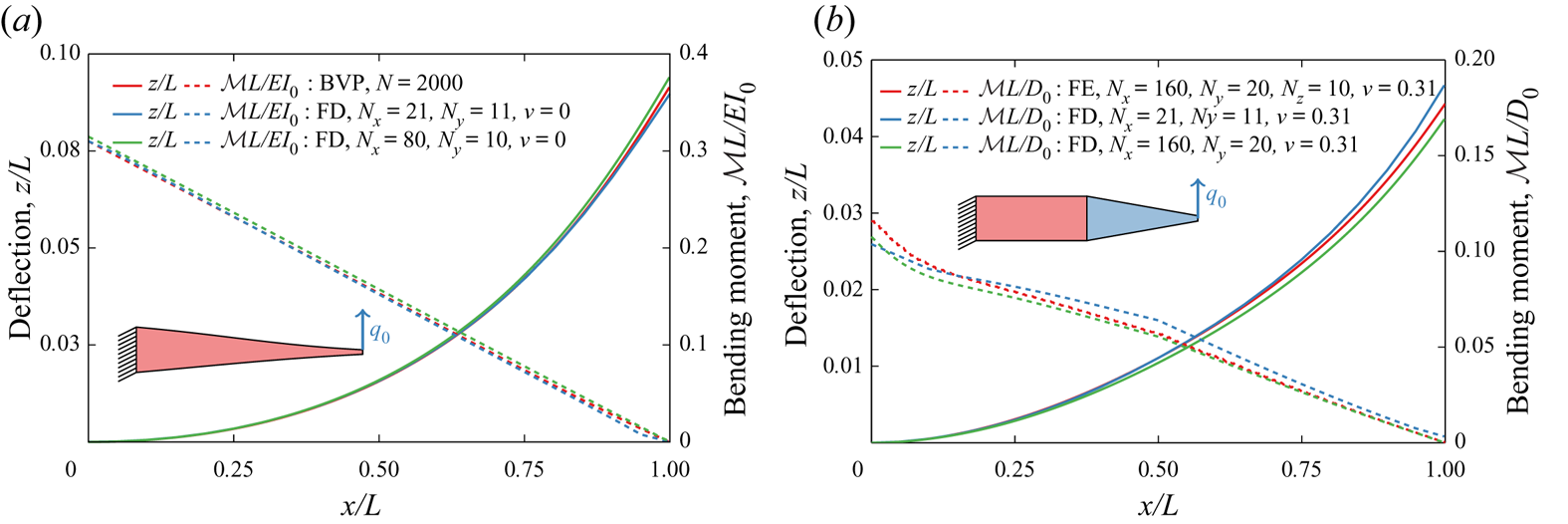
Figure 2. Static deflection under a non-dimensional load  $q_0 L^{2} / {D}_0 = 0.1$ of (a) a linearly tapered end-loaded cantilevered beam with $b=5$ and $\nu = 0$, and (b) a beam composed of uniform and linearly tapered sections with $b=5$ and $\nu = 0.31$.
In figure 2(b), we validate the FD solver using a three-dimensional solution obtained with the finite elements (FE) method using COMSOL Multiphysics. We consider a cantilever beam with  $\nu = 0.31$ that has two sections of equal length. The clamped half of the plate has a uniform thickness, while the other half is linearly tapered with a tapering ratio $b=5$. For the FE solver we use a mesh with $160 \times 20$ nodes, while for the FD solver we use meshes with $160 \times 20$ and $21 \times 11$ nodes. The FD and FE solutions show close agreement. Note that, for a non-zero Poisson ratio, the bending moment shows nonlinear behaviour near the root due to non-negligible two-dimensional effects at the clamped boundary.
The plate oscillations in a viscous fluid are governed by the Reynolds number  $Re = {\rho U_c L}/{\mu }$, and the mass ratio $\chi = {\rho W}/{\rho _s h_a}$, with $U_c = L/\tau$ being the characteristic velocity. The hydrodynamic performance of the plate is characterized by the dimensionless period-averaged thrust $\mathcal {F}$, power $\mathcal {P}$ and efficiency $\eta = \mathcal {F} / \mathcal {P}$, where the first two parameters are expressed in terms of the characteristic force $\frac {1}{2}\rho W L U_c^{2}$ and the characteristic power $\frac {1}{2}\rho W L U_c^{3}$. The thrust is computed by integrating the local hydrodynamic force in the $x$-direction acting on the surface of the plate. The overall propulsor length is set to $L = 50$ with $L_a=L_p=0.5L$ and $\mathcal {A}_R = 2.5$. Unless specified otherwise we use the tapering ratio $b=5$. We set the dimensionless bending moment $M_0 = 0.1$. We also set the fluid density $\rho =1$, fluid viscosity $\mu =1.25\times 10^{-3}$ and oscillation period $\tau = 2000$, leading to $Re = 2000$ and $\chi = 5$. The fine and coarse fluid grids, respectively, measure $4L \times 3L \times 3L$ and $8L \times 6L \times 8L$, with respective spacing $\varDelta _f = 1$ and $\varDelta _c = 2$. The plate is discretized with 21 FD nodes in the length and 11 FD nodes in the width, resulting in $\varDelta _x = 2.381$ and $\varDelta _y = 1.82$. To ensure that the flow reaches a steady state, simulations are performed for 40 periods of plate oscillations. Note that all dimensional values are given in LBM units.
4. Results and discussion
4.1. Acoustic black hole
Mironov (Reference Mironov1988) showed that, for tapered beams of finite length with thickness smoothly decreasing as  $h : x \longmapsto \varepsilon x^{n}, n \in \mathbb {N}^{*}$, the wavenumber goes to infinity. This suggests that when flexural waves propagate along an elastic plate with a thickness gradually decreasing to zero, they slow down and increase in amplitude. Since the wave velocity decreases to zero as the thickness vanishes, flexural waves propagating along the plates never reach the plate end and, therefore, do not reflect. Note that, in this system, the lack of wave reflection is solely due to the wave's inability to reach the tapered end in a finite time and is not related to the absorption or damping of the wave. This suppression of flexural wave reflection results in a region where waves are trapped that is referred to as an ABH. Thus, ABH prevents the wave reflection resulting in the formation of travelling waves and the suppression of standing waves.
In practice, manufacturing a plate with a zero-thickness tip is not possible due to physical and structural limitations. When the plate tip thickness is not zero, reflections occur at the tip, substantially reducing the ABH effect (Mironov Reference Mironov1988; Pelat et al. Reference Pelat, Gautier, Conlon and Semperlotti2020). With a tapering ratio  $b = 5$, the transit time $\mathcal {T} = \int _0^{L} {{\rm d}x} / [ 2 ({E \omega ^{2}}/{12 \rho })^{{1}/{4}} \sqrt {h(x)} ]$ increases by approximately 20 %–25 % compared with a plate with uniform thickness (figure 3a).

Figure 3. (a) Total transit time and (b) smoothness criterion for propulsors with passive attachments at resonance  $r=1$.
The ABH theory uses the regularity condition on the thickness, namely the Wentzel–Kramers–Brillouin–Liouville–Green condition (Liouville Reference Liouville1836; Green Reference Green1838; Brillouin Reference Brillouin1926; Kramers Reference Kramers1926; Wentzel Reference Wentzel1926), that postulates that the local wavenumber varies slowly over the wavelength  $({1}/{k^{2}})({{\rm d} k}/{{\rm d}x}) \ll 1$, where $k$ is the wavenumber. This smoothness criterion is shown in figure 3(b) for the tapering shapes considered in this work. The interface between the uniform plate and the tapered attachment displays a jump in smoothness since the thickness is not differentiable at this point. Furthermore, steeper attachment shapes lead to less smooth transitions between the active and passive sections. The smoothness discontinuity can lead to wave reflections at the interface between the active section and the attachment, thereby diminishing the ABH effect and the formation of travelling waves. Thus, the smoothness needs to be minimized to maximize $\mathcal {T}$.
4.2. Frequency response
Figure 4 shows the Bode diagram for resonance oscillations of propulsors with different attachments with the tapering ratio  $b = 5$. The solid symbols represent the response at the end of the active section, whereas the empty symbols show the response at the tip of the attachment. For all attachments, the root-mean-square (r.m.s.) velocity at the end of the active section shows a resonance maximum at $r=1$ (figure 4a). The tip of the tapered sections displays a similar velocity dependence with the exception of the exponential attachment that has velocity continuously increasing with the frequency ratio $r$. Furthermore, we find that the ‘steeper’ tapering shapes result in higher tip velocities for the entire range of considered frequency ratios. For instance, at resonance the exponential tapering nearly doubles the tip velocity compared with the uniform plate. The enhancement of the tip velocity is even more significant for post-resonance frequencies. While the velocity of the uniform plate rapidly decreases for $r>1$, the exponential tapering leads to a velocity increase. Moreover, the parabolic concave and linear tapered attachments display a velocity increase for $r > 2$. This is in contrast to the uniform plate attachment for which the velocity steadily decreases post-resonance with increasing $r$. Thus, our results for tapered attachments indicate that the tip velocity increases with increasing ‘steepness’ of the attachment and the high tip velocity is maintained for a wide range of frequency ratios.
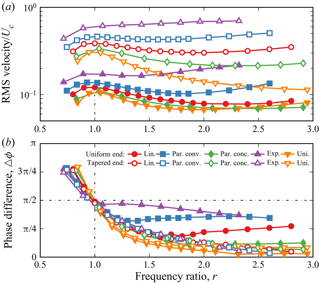
Figure 4. (a) The r.m.s. velocity and (b) phase difference of the internally actuated plate with several tapered passive attachments. The solid and empty symbols show the values for the ends of the tapered and uniform sections, respectively.
At resonance  $r = 1$, the phase difference $\varDelta \phi = {\rm \pi}/2$ and approaches asymptotically either $0$ or ${\rm \pi}$ away from the resonance, with the slope being a function of the overall damping (figure 4b). Note that $\varDelta \phi$ is defined as the phase difference between the input signal and the tip velocity. For the tapered attachment tip shown by the empty symbols, $\varDelta \phi$ overlaps for all tapering shapes. Conversely, $\varDelta \phi$ at the interface between the uniform and tapered sections, shown by the solid symbols, deviates from the uniform plate for $r>1$. The steeper the tapering the earlier the deviation occurs.
4.3. Bending pattern
In figure 5(a), we show the bending pattern of the internally actuated plate with a uniform attachment actuated at resonance. The reflection at the attachment tip creates a standing wave characterized by in phase oscillations along the entire propulsor length. As shown in figure 5(b), the propulsor with an exponential attachment yields noticeably different bending patterns. Although the plate propulsor is actuated at resonance, the dynamic response combines travelling and standing waves. Due to the ABH effect, the tapered attachment impedes waves from reflecting at the tip, and thus, its bending pattern is characterized by a mix of standing and travelling waves.

Figure 5. Bending patterns of propulsors at resonance  $r=1$ with (a) uniform attachment and (b) exponential attachment. Bending patterns of propulsors off resonance $r=2$ with (c) uniform attachment and (d) exponential attachment. The insets show the attachment curvature. The solid blue lines correspond to $0< t/\tau \leq 0.5$, while the dashed red lines correspond to $0.5< t/\tau \leq 1$. Also see supplementary movie 1 available at https://doi.org/10.1017/jfm.2022.470.
In the insets in figures 5(a) and 5(b), we plot the curvature profiles  $\kappa (x) = z''(x)/[1+{z'}^{2}(x)]^{3/2}$ in the respective attachments at $r = 1$. The curvature pattern of the uniform attachment is typical for a passive plate with a monotonic envelope and a vanishing curvature at the free end. Conversely, the curvature of the exponentially tapered attachment displays a local maximum around $x/L \simeq 0.8$. Moreover, the maximum curvature amplitude is approximately six times that of the uniform attachment.
Off-resonance bending patterns at  $r = 2$ for propulsors with uniform and exponential attachments are shown in figures 5(c) and 5(d), respectively. The bending patterns are characteristic of off-resonance oscillations with non-overlapping bending profiles for the up and down strokes, indicative of a combination of travelling and standing waves. The exponential attachment yields an approximately four times greater maximum tip displacement compared with the uniform attachment. Furthermore, the tip displacement of the exponential attachment at $r = 2$ exceeds its tip displacement at resonance at $r=1$.
The tapering shape of the attachment significantly impacts the form of the oscillation envelope as measured by the curvature in the insets in figures 5(c) and 5(d). For the uniform attachment, the maximum curvature gradually decreases with  $x$ with a maximum $\kappa _{max} L \simeq 0.18$ at $x/L = 0.5$, while the exponential attachment displays a maximum $\kappa _{max} L \simeq 1.5$ at $x/L \simeq 0.8$. Due to the low bending stiffness at the tip, the same internal moment input leads to a greater curvature and, therefore, deformation of the tapered attachment compared with the uniform attachment.
4.4. Travelling-to-standing wave ratio
Consider a travelling wave  $u_t(x,t) = A_t \cos kx \cos \omega t + A_t \sin kx \sin \omega t$ and a standing wave $u_s(x,t) = A_s \cos kx \cos \omega t$. A general wave resulting from the superposition of a standing and travelling wave is then given by $\hat {u}(x,t) = \cos (kx) \cos (\omega t) \pm \mathcal {S} \sin (kx) \sin (\omega t)$, where $\mathcal {S} = {A_t}/{(A_t+A_s)}$ is the travelling-to-standing wave ratio and $\hat {u}$ is amplitude-normalized velocity. The magnitude of $\mathcal {S}$ quantifies the fraction of the travelling wave in the superposition. The ratio is zero when the oscillations represent a standing wave and unity for a travelling wave. We use $\mathcal {S}$ to quantify the combination of travelling and standing waves resulting from the addition of a tapered attachment. Evaluation of $\mathcal {S}$ is based on the fitting a Hilbert transform onto an ellipse in the complex plane (Minikes et al. Reference Minikes, Gabay, Bucher and Feldman2005).
Figure 6 shows the dependence of  $\mathcal {S}$ on the frequency ratio $r$. We find that steeper tapering leads to a greater $\mathcal {S}$. Furthermore, as the frequency ratio increases, $\mathcal {S}$ increases with the rate depending on the tapering shape. For the exponential and parabolic convex shapes, $\mathcal {S}$ reaches maxima for $r \simeq 1.6$ and $r\simeq 2.4$, respectively. Past these frequencies, $\mathcal {S}$ decreases for both tapering shapes. We speculate that similar maxima exist for less ‘steep’ tapering shapes at frequencies that exceed those considered in our simulations. Although it is less ‘steep’, the parabolic convex attachment yields an approximately $10\,\%$ higher $\mathcal {S}$ than the exponential attachment. Similarly, $\mathcal {S}$ due to linear tapering increases steadily and nearly surpasses the exponential $\mathcal {S}$ for sufficiently large $r$. These observations indicate that the sharper tapering causes a faster increase in $\mathcal {S}$ with $r$, however, the maximum value is not directly defined by the tapering steepness. This can be related to a smoother transition at the interface between the active and passive segments for the propulsor with the parabolic convex attachment compared with the exponential attachment (figure 3b). A sharp change at the interface between active and passive segments can lead to spurious modes and reflections affecting the formation of travelling waves. Overall, the significant increase in $\mathcal {S}$ shows that tapered attachments with non-vanishing tip thickness are an effective solution to maintaining travelling waves in plate propulsors of finite length.

Figure 6. Travelling-to-standing wave ratio  $\mathcal {S}$ as a function of the frequency ratio $r$ for internally actuated plate propulsors with different attachments.
4.5. Hydrodynamic performance
In figure 7(a), we plot the dimensionless thrust  $\mathcal {F}$ as a function of the frequency ratio $r$ for propulsors with different passive attachments. For the uniform attachment, the thrust is maximized at resonance and rapidly decreases off resonance, which correlates with the plate r.m.s. velocity (figure 4). By comparing the thrust for different attachments at $r=1$, our results demonstrate that the attachments with steeper tapering generate more thrust, with the maximum $\mathcal {F}$ yielded by the exponential attachment. The parabolic concave and linear tapered attachments perform similarly to the uniform attachment. The thrust produced by the exponential and parabolic convex attachments noticeably exceeds the $\mathcal {F}$ generated by the other attachments. In the case of the exponential attachment, the local maximum thrust does not occur near the first resonance frequency; rather, the thrust steadily increases with the frequency ratio until it peaks at $r \simeq 1.8$. For the parabolic convex attachment, the maximum thrust is generated at $r \simeq 2.4$. Note that the maximum thrust generated by the propulsor with the exponential attachment is nearly 8 times greater than the maximum thrust of the propulsor with the uniform thickness. Thus, thickness tapering can drastically enhance the hydrodynamic thrust.

Figure 7. (a) Thrust, (b) power and (c) efficiency as a function of the frequency ratio  $r$ for internally actuated plates with different tapered attachments.
In figure 7(b), we plot the dimensionless power input  $\mathcal {P}$ as a function of $r$. We find that tapered attachments require higher power than the attachment with uniform thickness. For instance, the exponential attachment requires more than four times the power input of the uniform attachment at $r=1$. Indeed, the tapered attachment results in a higher tip displacement and a greater deformation envelope (figures 5). The larger deformation envelope leads to an increased fluid displacement and viscous dissipation magnifying the power consumption.
In figure 7(c), we plot the propulsor efficiency  $\eta$ as a function of $r$. In the case of the uniform passive attachment, the efficiency decreases until it reaches a local minimum at $r \simeq 1.7$. The efficiency then slightly increases to a local maximum at $r \simeq 2$ followed by a steep decrease. In other words, in the case of the uniform attachment, the actuation frequency has to be precisely tuned to achieve the optimal efficiency. For the tapered attachments, the efficiency is near the minimum at the resonance, with the magnitude close to that of the uniform propulsor. However, the tapered attachments outperform the uniform attachment for driving frequencies past the resonance. For instance, the parabolic convex attachment yields $\eta \simeq 0.55$ for $r=2.4$, which is nearly 1.4 times greater than the maximum efficiency of the uniform attachment. Interestingly, the parabolic convex attachment, while it does not have the ‘steepest’ tapering, outperforms the exponential attachment. This is correlated with the higher values of $\mathcal {S}$ for the parabolic convex attachment (figure 6), indicating that travelling waves enhance the propulsor hydrodynamic efficiency.
4.6. Scaling metrics
In figure 8(a), we plot the relationship between the dimensionless thrust  $\mathcal {F}$ and the dimensionless tip displacement $d/L$ for attachments with different shapes and two tapering ratios. The colour of the markers indicates the magnitude of the frequency ratio r. Our results show that the thrust scales with the tip displacement as $\mathcal {F} \sim d^{3}$, independently of the tapering shape and the tapering ratio $b$ (left inset in figure 8a). We find that steeper tapering shapes enable greater tip displacement, which ultimately, leads to higher thrust. In other words, tapered attachments can be used to maximize the tip displacement for a wide range of actuation frequencies, which in turn enhances the hydrodynamic thrust. The dependence of the thrust on tip displacement is consistent with the literature data for uniform propulsors (Lighthill Reference Lighthill1970; Dewey et al. Reference Dewey, Boschitsch, Moored, Stone and Smits2013; Floryan et al. Reference Floryan, Van Buren, Rowley and Smits2017; Ayancik et al. Reference Ayancik, Zhong, Quinn, Brandes, Bart-Smith and Moored2019; Lagopoulos, Weymouth & Ganapathisubramani Reference Lagopoulos, Weymouth and Ganapathisubramani2019). Furthermore, we find that our simulation results for $\mathcal {F}$ are in good agreement with the scaling derived by Gazzola, Argentina & Mahadevan (Reference Gazzola, Argentina and Mahadevan2014) and confirmed experimentally by Gibouin et al. (Reference Gibouin, Raufaste, Bouret and Argentina2018) (right inset in figure 8a). This result indicates that our simulations follow the same scaling behaviour that is universal for aquatic animals at the limit of large $Re$.
$Re$.

Figure 8. (a) Thrust as a function of tip displacement. (b) Power as a function of the dimensionless maximum displacement area. The data are for internally actuated propulsors with different passive attachments for  $b=2.5$ and $b=5$.
Previous studies indicate that the power input is proportional to the relative motion between the fluid and the oscillating plate leading to viscous dissipation (Yeh & Alexeev Reference Yeh and Alexeev2014; Demirer, Oshinowo & Alexeev Reference Demirer, Oshinowo and Alexeev2021a; Demirer et al. Reference Demirer, Wang, Erturk and Alexeev2021b). To estimate this power metric, we evaluate the maximum displacement area of the propulsor  $\mathcal {A} = \max _t ({1}/{L^{2}}) \int _0^{L} {w(x,t)\,{{\rm d}x}}$, where $w$ is the displacement of the plate along the centreline. In figure 8(b), we plot the mean dimensionless power $\mathcal {P}$ as a function of $\mathcal {A}$ for propulsors with different attachments and $b$. We find that all data collapse on a master curve, indicating a direct relationship between the power and the displacement area such that $\mathcal {P} \sim \mathcal {A}^{3}$ (inset in figure 8b). We conclude that minimizing the maximum displacement area decreases the power input.
The propulsor efficiency  $\eta$ is defined as the ratio between the dimensionless thrust $\mathcal {F}$ and the dimensionless power $\mathcal {P}$ that are, respectively, proportional to $d$ and $\mathcal {A}$. In figure 9(a), we plot $\eta$ as a function of $\mathcal {A}L / d$. The colour of the markers indicates the magnitude of $\mathcal {F}$. We find that the efficiency is correlated with $\mathcal {A}L / d$, and that a lower magnitude of this ratio leads to a higher efficiency. The low values of $\mathcal {A}L / d$, however, do not ensure high $\mathcal {F}$. In a relatively narrow band of $\mathcal {A}L / d$ between 14 and 15, $\mathcal {F}$ for different propulsors ranges from 0.025 to 0.2. Indeed, a low $\mathcal {A}L /d$ can correspond to different values of $d$. Whereas larger $d$ results in significant $\mathcal {F}$, low $d$ produces weak propulsion even when the bending pattern is characterized by a sufficiently low $\mathcal {A}$ to yield high $\eta$.

Figure 9. Efficiency as a function of (a) the ratio between the maximum displacement area and tip displacement and (b) the travelling-to-standing wave ratio. (c) Travelling-to-standing wave ratio as a function of the ratio between the maximum displacement area and tip displacement. The data are for internally propulsors with different passive attachments for  $b=2.5$ and $b=5$.
Since the hydrodynamic efficiency is associated with travelling waves (Cui et al. Reference Cui, Yang, Shen and Jiang2018), in figure 9(b) we plot  $\eta$ as a function of the travelling-to-standing wave ratio $\mathcal {S}$ with the marker colour indicating $\mathcal {F}$. At low $\mathcal {S}$, we find a significant spread of the efficiency without a clear trend that includes propulsors with tapered and uniform attachments. For high values of $\mathcal {S}$, there is a direct correlation between the high propulsion efficiency and $\mathcal {S}$ such that $\eta \sim \mathcal {S}^{0.4}$ (inset in figure 9b). Moreover, high $\mathcal {S}$ yields high thrust output. Indeed, for $\mathcal {S}>0.5$ the thrust is in the range between 0.05 and 0.2.
When we plot  $\mathcal {S}$ as a function of the ratio $\mathcal {A}L/d$ (figure 9c), we find that the data from different simulations collapse into a single curve where at the lower spectrum of $\mathcal {A}L/d$ the higher values of $\mathcal {S}$ yield greater thrust. Thus, larger values of $\mathcal {S}$ result in oscillations with lower $\mathcal {A}L/d$ and, at the same time, higher $d$ yielding greater $\mathcal {F}$ (figure 8a). Since large $\mathcal {S}$ are associated with the ABH effect at the tapered attachments (figure 6), we conclude that propulsors with such attachments exhibit the travelling wave propulsion leading to high $\eta$ and $\mathcal {F}$.
4.7. Flow patterns
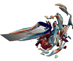
As the plate deforms, the relative motion between the plate and the fluid results in vorticity that is the most significant along the trailing edge and side edges. The vorticity is associated with hydrodynamic propulsion and dissipation (Anderson et al. Reference Anderson, Streitlien, Barrett and Triantafyllou1998; Nauen & Lauder Reference Nauen and Lauder2002; Alben Reference Alben2009; Michelin & Llewellyn Smith Reference Michelin and Llewellyn Smith2009; Yeh & Alexeev Reference Yeh and Alexeev2014; Paraz, Schouveiler & Eloy Reference Paraz, Schouveiler and Eloy2016; Yeh & Alexeev Reference Yeh and Alexeev2016b). Figures 10 and 11 show representative contours of  $Q$-criterion (the second invariant of the velocity gradient tensor) coloured by the magnitude of the $y$-component of the vorticity for propulsors with the uniform and exponential attachments, respectively. The flow structures in these figures are typical of oscillating plate propulsors (Facci & Porfiri Reference Facci and Porfiri2013; Demirer et al. Reference Demirer, Wang, Erturk and Alexeev2021b) with the formation of trailing edge vortices (TEVs) and side edge vortices (SEVs). While the TEVs generate thrust by forming a jet in the wake, the SEVs are typically detrimental to the propulsor hydrodynamic efficiency by dissipating energy without creating propulsion. Comparing the two attachments at resonance $r=1$ (figures 10(a) and 11(a)), the exponential attachment produces a greater amount of vorticity that can be attributed to an increased amplitude of the trailing edge displacement.

Figure 10. Snapshots of normalized  $\mathcal {Q}$-criterion contours ( $\mathcal {Q} \tau ^{2} = 5$) coloured by $y$-component of the vorticity for the propulsors with the uniform attachment (a) at resonance $r=1$ and (b) off resonance $r=2$. The snapshots are for (i) $t/\tau = 0$, (ii) $t/\tau = 0.25$, (iii) $t/\tau = 0.5$ and (iv) $t/\tau = 0.75$. See supplementary movie 2.

Figure 11. Snapshots of normalized  $\mathcal {Q}$-criterion contours ( $\mathcal {Q} \tau ^{2} = 10$) coloured by $y$-component of the vorticity for the propulsors with the exponential attachment (a) at resonance $r=1$ and (b) off resonance $r=2$. The snapshots are for (i) $t/\tau = 0$, (ii) $t/\tau = 0.25$, (iii) $t/\tau = 0.5$ and (iv) $t/\tau = 0.75$. See supplementary movie 3.
The difference between the vorticity fields of the two propulsors is even more dramatic at the post resonance frequency  $r=2$ (figures 10(b) and 11(b)). At $r=2$ the propulsor with the uniform attachment exhibits significantly lower deformation than at resonance, yielding a relatively low amount of vorticity generated by the propulsor. On the other hand, the deformation amplitude of the exponential propulsor at $r=2$ exceeds the amplitude at resonance, and so does the vorticity that significantly exceeds that of the propulsor with the uniform attachment at $r=2$. This explains the greater hydrodynamic performance of the propulsor with the tapered exponential attachment that takes place not only at resonance, but also for post-resonance actuation frequencies.
To examine the impact of travelling waves on the propulsor hydrodynamics and the emerging flow patterns, we compare two propulsor configurations with similar tip displacement  $d$ and displacement area $\mathcal {A}$, but different magnitude of travelling-to-standing wave ratio $\mathcal {S}$. Specifically, in figures 12(a) and 12(b), we show propulsors with the parabolic convex attachments at $r=1.2$ and $r=2.4$, respectively. The parameters of these two cases are presented in table 1. At the lower frequency ratio, the plate oscillations are mostly a standing wave ( $\mathcal {S} \simeq 0.2$), whereas at the higher frequency ratio, the plate exhibits travelling waves propagating along the propulsor ( $\mathcal {S} \simeq 0.9$). The oscillations with travelling waves produce higher thrust with lower input power. As a result, the oscillations at $r=2.4$ are twice as efficient than at $r=1.2$. Figure 12 shows that both these configurations generate similar levels of vorticity with dominant TEVs and SEVs, although oscillations at $r=2.4$ produce somewhat lower mean enstrophy $\mathcal {E} = {\boldsymbol{\omega}} \times {\boldsymbol{\omega}} \tau ^{2}$ that quantifies the intensity of viscous dissipation by the plate (table 1). We find that the dynamics of the vortical fields is noticeably different for the oscillations characterized by standing and travelling waves. For standing wave oscillations at $r=1.2$, there are relatively weak interactions between TEVs and SEVs. On the other hand, for travelling wave oscillations at $r=2.4$, the waves propagating along the propulsor length transport SEVs towards the trailing edge where SEVs interact with TEVs.

Figure 12. Snapshots of normalized  $\mathcal {Q}$-criterion contours ( $\mathcal {Q} \tau ^{2} = 10$) coloured by $y$-component of the vorticity for the propulsors with the parabolic convex attachment (a) at $r=1.2$ and (b) at $r=2.4$. The snapshots are for (i) $t/\tau = 0$, (ii) $t/\tau = 0.25$, (iii) $t/\tau = 0.5$ and (iv) $t/\tau = 0.75$. See supplemental movie 4.
Table 1. Hydrodynamic parameters of the parabolic convex attachment at  $r=1.2$ and $r=2.4$.

In figures 13(a) and 13(b), we show the out-of-plane component of the vorticity  $\omega _y$ generated by the parabolic convex propulsors at $r=1.2$ and $r=2.4$, respectively. The vorticity is shown at the mid-plane of the plates. The relative motion between the plate and the flow results in vortices generated about the midchord and shed towards the tip. The alternating clockwise and counter-clockwise shedding structure is characteristic of a reverse von Kármán vortex street (Anderson et al. Reference Anderson, Streitlien, Barrett and Triantafyllou1998; Von Ellenrieder, Parker & Soria Reference Von Ellenrieder, Parker and Soria2003; Lentink et al. Reference Lentink, Muijres, Donker-Duyvis and Van Leeuwen2008). The rotation of the vortices induces an increase in the streamwise component of the momentum, and thus enhances the propulsion. The downstream vortex structures of the two oscillation regimes are distinctively different. For the travelling wave oscillations at $r=2.4$, a bifurcating wake develops downstream of the propulsor due to greater vortex intensity. As vortices shed streamwise, they stretch and, due to significant cross-stream velocity, break into smaller vortices moving orthogonal to the streamwise direction forming a bifurcating wake.

Figure 13. Snapshots of normalized vorticity field at (a)  $r=1.2$ and (b) $r=2.4$ for the parabolic convex attachment. The snapshots are for (i) $t/\tau = 0$, (ii) $t/\tau = 0.25$, (iii) $t/\tau = 0.5$ and (iv) $t/\tau = 0.75$. See supplemental movie 5.
The bifurcating wake structure is further confirmed in figure 14(a,b), where we plot the time-averaged velocity field for the propulsor with parabolic convex attachment actuated at  $r=1.2$ and $r=2.4$. The figure reveals a narrowing jet in the streamwise direction for $r=1.2$, whereas at higher $r=2.4$ the propulsor oscillations result in a pair of narrowing jets at an acute angle with the streamwise direction. Travelling waves cause a faster mean flow speed along the propulsor, enhancing propulsor performance (figure 14c). This flow structure is characteristic of undulating elastic propulsors (Borazjani & Sotiropoulos Reference Borazjani and Sotiropoulos2008, Reference Borazjani and Sotiropoulos2009; Godoy-Diana et al. Reference Godoy-Diana, Marais, Aider and Wesfreid2009) and fish swimming (Tytell & Lauder Reference Tytell and Lauder2004; Hultmark, Leftwich & Smits Reference Hultmark, Leftwich and Smits2007; Wu Reference Wu2011), where bifurcating wakes emerge at higher Strouhal numbers $\textit {St}$ and are associated with enhanced propulsion efficiency.

Figure 14. Time-averaged velocity field at (a)  $r=1.2$ and (b) $r=2.4$ for the parabolic convex attachment. (c) Normalized $x$-component of the period-averaged velocity profiles at various positions along the plate and wake for $r=1.2$ and $r=2.4$.
5. Summary
We use three-dimensional computer simulations to probe the hydrodynamic performance of bio-mimetic elastic propulsors with tapered thickness. The propulsors are composed of an active section at the base inducing the propulsor periodic oscillations in an incompressible Newtonian fluid, and a passive attachment with tapered thickness. The tapering aims to create the ABH effect leading to a wave speed decrease towards the propulsor trailing edge, thereby suppressing the flexural wave reflection and promoting the formation of travelling waves. As a result, the propulsors with ABH exhibit beating patterns that feature travelling flexural waves propagating along the propulsor length. By altering the propulsor thickness profile, the strength of ABH can be regulated yielding propulsors with different ratios between the travelling and standing waves in their beating patterns. We find that the travelling-to-standing wave ratio is approximately zero for uniformly thick propulsors, indicating that the propulsor oscillations are standing flexural waves, whereas for exponential and parabolic convex tapered propulsors, the value of the ratio approaches unity, indicating the dominance of travelling waves in the beating patterns. We directly evaluate and compare the hydrodynamic performance of propulsors with beating patterns that exhibit different levels of travelling-to-standing wave ratios.
Our simulations reveal that tapered propulsors with ABH significantly outperform propulsors with uniform thickness in terms of the hydrodynamic thrust and efficiency for a broad range of actuation frequencies, including resonance and off-resonance oscillations. Tapering increases the magnitude of the tip displacement compared with uniform propulsors, thereby leading to greater thrust that is directly proportional to the tip displacement magnitude. Furthermore, tapered propulsors with ABH leading to high travelling-to-standing wave ratios demonstrate a superior efficiency defined as the ratio of the dimensionless thrust and power. We show that the input power is proportional to the amount of fluid displaced by an oscillating propulsor. For uniform propulsors with standing wave oscillations, the frequency regimes leading to reduced input power also result in the lower tip displacement magnitude and, therefore, weak thrust. Thus, for uniform propulsors there is a trade-off between high thrust and high efficiency. By contrast, travelling wave propulsion yields bending patterns with relatively low input power while maintaining a high tip displacement amplitude.
We examine the flow field and vortical structures generated by propulsors with standing and travelling waves and show that standing waves yield a reverse von Kármán vortex street, whereas travelling waves generate a bifurcating wake downstream of the propulsor. The travelling wave oscillations with bifurcating wake lead to significantly higher propulsion and efficiency than standing wave oscillations of comparable oscillation magnitude. We attribute this to the increased fluid transport by the travelling waves propagating along the propulsor length. Furthermore, travelling waves increase interactions among SEVs and TEVs by transporting SEVs towards the trailing edge. Whereas, for standing wave oscillations, SEVs do not participate in generating forward thrust, the interaction of SEVs with TEVs by travelling waves enhances the vorticity and, therefore, the momentum transfer facilitating propulsion, similar to the positive reinforcement observed for leading edge vortices (Lewin & Haj-Hariri Reference Lewin and Haj-Hariri2003; Guglielmini & Blondeaux Reference Guglielmini and Blondeaux2004). The unique ability of tapered propulsors with ABH to generate high thrust with high efficiency makes them excellent candidates for designing highly efficient bio-mimetic robotic swimmers.
Our results support the observations that the travelling wave-based anguilliform swimming of fishes such as eels and lampreys is beneficial for the efficient locomotion (Lighthill Reference Lighthill1970; Borazjani & Sotiropoulos Reference Borazjani and Sotiropoulos2010). Our simulations offer an explanation for the better energetic performance reported for travelling wave-based swimming over standing wave-based swimming at lower  $Re$ (Tytell Reference Tytell2010; Tytell et al. Reference Tytell, Borazjani, Sotiropoulos, Baker, Anderson and Lauder2010). On the other hand, we do not find an advantage of standing wave oscillations over travelling wave oscillations in generating propulsion thrust, suggesting that travelling waves are beneficial for thunniform swimming. We note that several aspects of our study can limit the extent to which our results can be applied to biological fish. Here, we explore swimming at $Re =2000$, whereas thunniform and ostraciiform swimming are more typical for faster fish with higher $Re$ (Lindsey Reference Lindsey1978; Sfakiotakis, Lane & Davies Reference Sfakiotakis, Lane and Davies1999). We consider oscillations with a wavelength that is approximately twice longer than the propulsor length as typical for thunniform fish, whereas angulliform fish have a wavelength approximately half of the fish body length (Smits Reference Smits2019). Furthermore, we consider propulsors with simplified rectangular geometry and disregard the hydrodynamic effects of the fish body. Finally, the form of fish swimming is tightly related to the fish physiology and, in particular, the muscle function (Webb Reference Webb1994; Müller & Van Leeuwen Reference Müller and Van Leeuwen2006; Cohen & Boyle Reference Cohen and Boyle2010), which makes a direct hydrodynamic comparison between different forms of fish swimming more challenging and points to the need for future studies using more elaborate models.
Supplementary movies
Supplementary movies are available at https://doi.org/10.1017/jfm.2022.470.
Acknowledgements
Stimulating discussions with Dr R. Godoy-Diana are gratefully acknowledged.
Funding
We thank the National Science Foundation (CBET-1705739) for financial support. The work used the Extreme Science and Engineering Discovery Environment (XSEDE) provided through Award TG-DMR180038.
Declaration of interests
The authors report no conflict of interest.


 Open access